Mixed-Convective Processes Within Seafloor Sediments Arising From Fresh Groundwater Discharge

Introduction

Subsea fresh groundwater discharge (SFGD) is the release of freshwater from seafloor sediments, and has been identified as an important means to transport dissolved nutrients to the ocean, thereby having a significant influence on marine ecology and benthic organisms (e.g., Johannes, 1980; Moore, 1999). Knowledge of the salinity patterns in subsea sediments is important for several reasons, including for the understanding of benthic ecosystems in regions of SFGD, and for the design of SFGD measurement approaches. The distribution of groundwater discharge to the sea depends on the characteristics of geological formations. Fresh groundwater discharge to intertidal zones is often associated with unconfined aquifers, whereas SFGD, occurring beyond the intertidal zone, typically requires low-permeability confining units that act to limit freshwater-seawater mixing that would otherwise occur near the shoreline (e.g., Jiao et al., 2015; Michael et al., 2016). Predictions of the extent of subsea fresh groundwater typically assume that the low-permeability layers that preserve freshwater and allow SFGD to occur are in direct contact with seawater (e.g., Kooi and Groen, 2001; Bakker et al., 2017; Solórzano-Rivas and Werner, 2018; Werner and Robinson, 2018; Solórzano-Rivas et al., 2019). However, the seafloor more often comprises high-permeability sediments (>50% of the global shelf sediments have high permeability; Riedl et al., 1972). Yet, this configuration has not been widely considered in studies of SFGD.

The occurrence of freshwater in high-permeability sediments overlain by seawater, as occurs when SFGD passes through permeable seafloor sediments, creates a mixed-convective condition. That is, flow processes are expected to be controlled by both buoyancy-driven flow (i.e., free convection) driven by water density differences and hydraulic-driven flow (i.e., forced convection) arising from groundwater heads in subsea sediments that exceed those of the sea. Thus, solute distributions in subsea aquifers may resemble those of other mixed-convective situations. However, studies of mixed-convective or free-convective processes where buoyancy is created by salinity gradients usually involve descending plumes of higher-density fluid that contaminate underlying lower-density groundwater (e.g., Webster et al., 1996; Smith and Turner, 2001; Stevens et al., 2009; Xie et al., 2011). Conversely, the upward movement of lower-density groundwater (e.g., as expected to arise during SFGD) is rarely explored in the solute transport context, although upward, buoyancy-driven groundwater flow has received significant attention in the field of heat transport and geothermal phenomena. For example, Kurylyk et al. (2018) utilized temperature-based methods to quantify submarine groundwater fluxes in seafloor sediments offshore of eastern Canada. However, their study suggested that the flow patterns inferred from seafloor temperature-depth profiles appear to be influenced by both density-driven and geothermal processes.

Perhaps the most pertinent prior investigation of mixed-convective transport accompanying SFGD is that of Moore and Wilson (2005), who were perhaps the first to recognize that SFGD may be driven by upward buoyancy forces. Based on temperature measurements of subsea groundwater (1.5 m below the seabed), Moore and Wilson (2005) interpreted that a sudden drop in the ocean temperature produced upward motion of warmer (i.e., less dense) groundwater to the ocean. However, previous research offers little guidance on the characteristics of free-convective or mixed-convective flow within seafloor sediments. In particular, whether mixed-convective flow within seafloor sediments can be characterized according to buoyancy theory developed for other unstable, solute transport conditions (e.g., leading to downward-moving fingers of higher density; e.g., Wooding et al., 1997) is unclear. This includes the application of several dimensionless variables that are used to categorize mixed-convective problems (e.g., Wooding et al., 1997; Simmons et al., 2010). Additionally, to our knowledge, no quantitative evaluation of mixed convection driven by the upward movement of lower-salinity groundwater has been reported in the literature. Rather, upward convection of lower-density groundwater has only been explored where buoyancy is created by temperature gradients (e.g., Irvine et al., 2015).

The aim of this study is to undertake a review of the existing buoyant theory, including non-dimensional numbers used to characterize mixed-convective flow, and explore whether this theory can be applied to SFGD through high-permeability seafloor sediments. A small number of highly idealized numerical simulations are used to provide an initial demonstration of freshwater-seawater mixing accompanying the rise of fresh buoyant plumes through permeable seafloor sediments. We expect that the upward movement of less-dense groundwater will show similar, albeit inverted, characteristics (e.g., buoyancy-driven fingers of freshwater) to the downward movement of more dense saltwater that has been comprehensively assessed in numerous prior investigations.

Conceptual Model

Two hypothetical conceptual models of SFGD are considered, both of which involve freshwater-seawater mixing within high-permeability, seabed sediments, as shown in Figure 1. Model A represents the situation where the seafloor sediments are underlain by a higher-permeability freshwater source, whereas Model B involves underlying sediments of lower permeability (i.e., an aquitard). The former is intended to reflect the situation of SFGD where an underlying aquifer sub-crops to the seafloor and is overlain by sand, while the latter represents SFGD passing through a leaky aquitard into more permeable seafloor sediments.

FIGURE 1

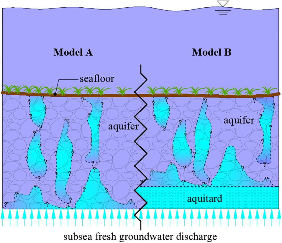
Figure 1. Two conceptual models of a subsea unconfined aquifer subject to SFGD. Blue is freshwater, and purple is seawater. Model A (left) involves sandy sediments overlying a subcropping, higher-permeability aquifer, and Model B represents an aquitard overlain by sand.

An important unknown for the conceptual models considered here is the distribution of freshwater within the seafloor sediments. While Figure 1 shows buoyant freshwater plumes that take the shape of fingers, similar to classic unstable flow patterns for downward free convection, freshwater-seawater mixing may alternatively be dominated by dispersive process (at least theoretically), leading to different salinity patterns to those represented in Figure 1. Most field studies of SFGD adopt methods that assume that SFGD occurs in a distributed form (i.e., presuming dispersive freshwater-seawater mixing in seafloor sediments), with devices located on the seafloor (i.e., seepage meters) in regular grid patterns (e.g., Taniguchi et al., 2003; Michael et al., 2005; Kurylyk et al., 2018). However, the buoyant freshwater plumes that are hypothesized here (Figure 1) may require alternative measurement strategies. For example, the spacing between, and size of, freshwater plumes, should they occur, may influence the deployment of seepage meters.

Although freshwater plumes within seafloor sediments are expected to behave similarly to the well-studied downward-moving saltwater plumes of prior studies (e.g., Xie et al., 2011), there are important differences between the conceptual model of Figure 1 and previous analyses of downward-moving plumes. Consider for example, the Elder problem (e.g., Elder et al., 2017), which was transformed to free-convective solute motion by Voss and Souza (1987), and is a common benchmarking problem for assessing numerical models. Various modifications of the Elder problem have occurred to explore other aspects of free convection problems. For example, Xie et al. (2010) introduced mechanical dispersion and changed the lower boundary condition to represent more realistic conditions, similar to the approach of Post and Kooi (2003). The conceptual model applied to SFGD (Figure 1) is, conceptually at least, an “inverse” of the solute-based Elder problem, where the aquifer is initially seawater-filled and a source of constant freshwater is introduced at the bottom boundary. The initial seawater conditions in the aquifer allow for the transience of salinization to be observed. However, the boundary conditions differ to those of the Elder problem to improve the representation of the expected SFGD process. That is, specified-head boundaries are imposed at the top (seawater) and the bottom (freshwater), whereas the Elder problem uses no-flow boundary conditions at all edges and specified hydraulic heads at the top corners (e.g., Guo and Langevin, 2002). Thus, the behavior of SFGD within seafloor sediments, under the conditions presented in Figure 1, cannot be inferred from previous studies. Further details of numerical models are provided in section “Numerical Simulation of SFGD.”

Review of Mixed-Density Non-Dimensional Numbers Applicable to SFGD Through Seafloor Sandy Sediments

The characterization of buoyancy-induced flow associated with unstable systems has been the subject of extensive research. One the most common non-dimensional numbers applied for this purpose is the Rayleigh number (Ra) (e.g., Simmons et al., 2010). Ra is the ratio between buoyancy forces (inducing instabilities in the form of solute fingers) and dispersion forces (tending to resist the formation of unstable solute fingers). When freshwater and seawater interact, Ra can be defined as (e.g., Post and Kooi, 2003):

$$Ra=\frac{K\mathrm{\Delta }\rho H}{{\rho }_{\text{f}}D}(1)$$

where K is the aquifer hydraulic conductivity (L T^–1), Δρ is the difference between the seawater (ρ_s) and freshwater (ρ_f) densities (M L^–3), H is the aquifer thickness (L), and D is hydrodynamic dispersion (L² T^–1). D is equal to the sum of molecular diffusion [D₀, (L² T^–1)] and mechanical dispersion, which is often simplified to α_Lv_L, where α_L is the longitudinal dispersivity (L) and v_L the advective flow velocity (L T^–1) (i.e., transverse dispersivity, α_T, is often neglected).

There are several alternative Ra formulations that have been reported in the literature. For example, some studies have presumed that D consists only of D₀, with mechanical dispersion neglected (e.g., Post and Kooi, 2003; Stevens et al., 2009; Simmons et al., 2010; Xie et al., 2011). These cases involve only free convection, i.e., hydraulic-driven convection is not considered. Alternative expressions for Ra have been developed for mixed-convection processes. For example, in mixed- convective problems examined by Simmons and Narayan (1997) and Smith and Turner (2001), both mechanical dispersion and molecular diffusion were included in their definitions of D. However, Simmons and Narayan (1997) adopted α_T and Smith and Turner (2001) adopted α_L in defining D. This study adopts the Smith and Turner (2001) definition of D.

The value of Ra has been used to predict the occurrence of unstable solute motion, typically in the form of solute fingers (e.g., Wooding et al., 1997). The critical Ra is defined as the threshold value at which buoyancy forces overcome dispersion forces that inhibit finger formation. This threshold value differs depending on conditions in which free convection occurs. For example, in the case of free convection in hydrogeological settings, Stevens et al. (2009) and Moore and Wilson (2005) refer to the critical Ra of 4π² (i.e., for the appearance of solute fingers) reported by Lapwood (1948) for temperature gradients in porous media. However, alternative critical Ra values are offered by other authors for free convection problems. According to van Reeuwijk et al. (2009), the historical incongruency in critical Ra estimates is related to such aspects as the numerical approach, governing equations, and slight differences in the initial conditions. They suggest that the critical Ra for free convection involving solutes is zero (in other words, solute fingers form without the need for a “dispersive boundary layer”; see below).

Applications of Ra theory to mixed-convective processes include the study of Simmons and Narayan (1997), who imposed linearly varying hydraulic heads across the top boundary, to induce lateral flow (i.e., flow parallel to the solute source boundary). The transverse dispersion created by this lateral flow was incorporated into the stabilizing dispersive force in assessing the critical Ra. By incorporating α_Tv_L in D, Simmons and Narayan (1997) include forced convection (i.e., v_L) in the definition of Ra. They found that the critical Ra ranged between 300 and 500 under these conditions. Smith and Turner (2001) considered a somewhat similar situation to that of Simmons and Narayan (1997), except fresh groundwater discharged to the upper solute boundary condition (i.e., the estuary) in Smith and Turner’s (2001) analysis of estuary-aquifer interaction. They obtained a critical Ra value of 5 for the onset of finger development. Solórzano-Rivas and Werner (2018) adopted the Smith and Turner (2001) formulation for the analysis of freshwater discharge through subsea aquifers, and found a critical Ra of about 2 for the salinization of submarine aquitards overlying fresh offshore aquifers. The application of Ra to mixed-convection problems introduces challenges in establishing general values for the critical Ra, given differences in the representation of forced convection in defining Ra across the abovementioned studies.

Wooding et al. (1997) analyzed the development of boundary layers within mixed-convective flow systems (i.e., where freshwater flows upwards towards a saltwater boundary). They derived an expression for the steady-state boundary layer thickness, δ (L), defined as the thickness of solute formed (by dispersion) in the presence of upward freshwater flow, q_z (L T^–1), as:

$$\delta =\frac{D_0}{q_{\text{z}}}(2)$$

Wooding et al. (1997) combined Equations 1 and 2, by equating H to δ (i.e., conceptually, this is the case where the boundary layer encompasses the entire aquifer thickness), to define a boundary-layer Rayleigh number, Ra_δ, namely:

$$R{a}_{\delta }=\frac{K\mathrm{\Delta }\rho \delta }{{\rho }_{\text{f}}D}(3)$$

The thickness of δ that leads to the onset of unstable solute fingers defines the critical Ra_δ. Wooding et al. (1997) undertook laboratory experiments using a Hele-Shaw cell to determine the critical Ra_δ, including different rates of lateral inflow at the right boundary and vertical outflow to the top, and using various inclination angles of the cell. They also performed numerical experiments that reproduced the two-dimensional flow and solute transport behavior observed in the Hele-Shaw experiment. From the laboratory and numerical experiments, they found Ra_δ values between 8.9 and 9.8, concluding that a good estimate for the critical Ra_δ is approximately 10.

Another widely used non-dimensional parameter for the characterization of mixed-convective processes is the mixed convection ratio (M). M describes the relationship between buoyancy-driven forces and hydraulic-driven forces as (e.g., Simmons et al., 2010):

$$M=\frac{\left(\frac{\mathrm{\Delta }\rho }{{\rho }_{\text{f}}}\right)}{\left(\frac{\mathrm{\Delta }h}{\mathrm{\Delta }l}\right)}(4)$$

where $\frac{\mathrm{△}h}{\mathrm{△}l}$ (-) is the hydraulic gradient over a distance Δl. An alternative expression for M, through substitution of Darcy’s Law, is given by Smith (2004), as:

$$M=\frac{K\mathrm{\Delta }\rho }{{\rho }_{\text{f}}{q}_{\text{z}}}(5)$$

By combining Equations 2 and 3, it is apparent that Ra_δ and the formulation for M given in Equation 5 are the same, i.e., M = Ra_δ. Surprisingly, this has not been reported previously to the authors’ knowledge. The implications of this are that critical values for Ra_δ also apply to M. However, there is no evidence that the equilibrium value of M = 1 suggested by Simmons et al. (2010) (whereby if M is larger than 1 the problem is said to be free-convection dominated, and forced convection is thought to be the dominant process if M is less than 1) has application in terms of Ra_δ. That is, Ra_δ = 1 has not been reported as a significant value previously. It follows that the onset of instabilities is not predictable through comparison of free and forced convective forces (i.e., through the use of M), as expected given the role that dispersion plays in instability initiation. Nevertheless, Stevens et al. (2009) applied M to the assessment of the occurrence of unstable solute fingering processes that accompany free convection on Padre Island (United States). The site experiences intense evaporation rates and shallow water table conditions, creating large density gradients and low horizontal hydraulic gradients. They found values of M, based on application of Equation 4, that were much larger than 1 (i.e., by one and two orders of magnitude), although numerical values of M were not reported. Stevens et al. (2009) interpreted unstable flow structures from resistivity surveys, although these were difficult to conclusively establish. Thus, the application of M to the prediction of unstable fingering remains unproven.

Numerical Simulation of SFGD

Here, the conceptual models illustrated in Figure 1 are adopted, except the situation is assessed whereby the sandy seafloor sediments are presumed to be originally filled with seawater. Numerical modeling, using SEAWAT (governing equations are found in Guo and Langevin, 2002; not repeated here for brevity), was used to assess two simple situations of SFGD through sandy seafloor sediments. The two cases (Models A and B; see Figure 2) involve contrasting mixed-convective forces arising from the inclusion or omission of an underlying aquitard. This is reflected in the corresponding values of Ra and Ra_δ, which are reported for each case and compared to previously reported critical values (Wooding et al., 1997; Smith and Turner, 2001) in section “Review of Mixed-Density Non-dimensional Numbers Applicable to SFGD Through Seafloor Sandy Sediments.” The calculation of Ra and M for Model B does not include the aquitard thickness (i.e., only H is regarded as per the Equation 1 definition).

FIGURE 2

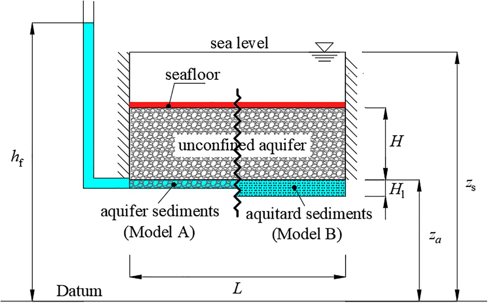
Figure 2. Conceptual models for the numerical implementation of SFGD through an unconfined subsea aquifer, where the left side shows sandy sediments overlying a subcropping, higher-permeability aquifer, and Model B represents an aquitard overlain by sand. Red and blue represent seawater and freshwater boundary conditions, respectively. The equivalent freshwater head at the base of the aquifer, when the aquifer is seawater-filled (i.e., the initial condition), is shown as h_f.

Figure 2 is a simplified section showing two possible configurations of a subsea aquifer subjected to SFGD, which is homogeneous, isotropic, and of length L (L) and thickness H (L). The upper boundary represents seawater immediately above the seafloor, simulated by a high hydraulic conductivity (i.e., 100,000 m/d) and a specified-head condition equal to z_s, assigned to the top row of the model. SEAWAT converts z_s to a constant pressure (Langevin et al., 2008) reflecting the column of overlying seawater, of density ρ_s. The solute concentration condition in this top layer depends on the flow direction, whereby seawater concentration (i.e., solute concentration = 1) was assigned to any inflowing water, whereas discharge to the sea occurs at the ambient groundwater concentration. This type of solute concentration condition avoids salt accumulation at the boundary in an unrealistic manner (i.e., upstream dispersion; Irvine et al., 2021) and is consistent with the approach of Solórzano-Rivas and Werner (2018). The lower freshwater boundary condition differs between Models A and B. In Model A, the lower boundary reflects a situation where an underlying layer of higher permeability occurs, containing freshwater. That is, there is no restriction to the entry of freshwater through the lower boundary of Model A, represented by a specified-head condition equal to h_f, which was converted to a constant pressure (by SEAWAT) based on a water density of ρ_f, as shown in Figure 2. In Model B, the lower boundary is composed of lower-permeability sediments (i.e., reflecting aquitard material) of thickness H_L, with the specified head h_f imposed on the bottom row of the model (i.e., the base of the aquitard). The solute concentration of the lower boundary for both Models A and B was set to freshwater (i.e., solute concentration = 0), although this depends on the flow direction in a similar manner to the upper boundary.

No-flow boundaries on the left and right edges of the model domain reflect mostly vertical flow processes. Post et al. (2007) and Langevin et al. (2008) offer the following formulation for vertical flow, q_z, under mixed-density conditions:

$$q_{\text{z}}=-K\left[\frac{\mathrm{\Delta }{h}_{\text{f}}}{\mathrm{\Delta }l}+\frac{{\rho }_{\text{a}}-{\rho }_{\text{f}}}{{\rho }_{\text{f}}}\right](6)$$

where ρ_a is the average density between ρ_s and ρ_f (M L^–3) and $\frac{\mathrm{△}{h}_{\text{f}}}{\mathrm{△}l}$ is the hydraulic gradient (in terms of equivalent freshwater heads) over a distance Δl.

The aquifer is assumed to be initially full of seawater but is underlain by a fresh groundwater source. The lower boundary head of both models is chosen so that the initial condition is hydraulically stable, primarily to reflect the free-convective situation (i.e., neglecting forced convection) that occurs in the Elder problem and its many variants, thereby providing opportunities to compare upward buoyancy-driven flow to the downward movement of solute fingers observed by others (e.g., Xie et al., 2011). That is, the hydraulic head of the fresh groundwater source is equal to the equivalent freshwater head, h_f, at the bottom of aquifer (at the beginning of each scenario). Considering an initial seawater hydrostatic condition, h_f is given by $\frac{{\rho }_{\text{s}}}{{\rho }_{\text{f}}}{z}_s-\frac{{\rho }_{\text{s}}-{\rho }_{\text{f}}}{{\rho }_{\text{f}}}{z}_a$ (where z_s and z_a are defined in Figure 2). Consequently, the only forces driving flow (initially) are buoyancy forces, because the hydraulic gradient is initially zero. Thus, at the beginning of the scenarios, Equation 6 reduces to:

$$q_{\text{z}}=-K\left[\frac{{\rho }_{\text{a}}-{\rho }_{\text{f}}}{{\rho }_{\text{f}}}\right](7)$$

Equation 7 is usually referred to as the convective velocity (e.g., Simmons et al., 2010). Vertical flow velocities in the numerical model, from the initial time-step, were found to be consistent with Equation 7 (results not shown for brevity).

Although the initial condition is a free convective condition, density changes due to the introduction of freshwater through the lower boundary create head gradients that induce boundary inflows, and the system becomes mixed convective. This differs to the free convection Elder problem, which is bounded by no-flow conditions, including the upper salt source boundary. Thus, although our situation is initially free convective, the situation becomes mixed convective during the course of simulations.

The model is a two-dimensional domain represented by a finite-difference grid of uniform discretization, both vertically and horizontally, of Δz = Δx = 0.1 m. Three cases are evaluated for each model (i.e., a total of six numerical simulations) to briefly explore the role of dispersion in the mixed-convective processes associated with SFGD through the seafloor sediments, namely a Base Case with α_L = 0.1 m, Case 1 with α_L = 0.5 m, and Case 2 with α_L = 1 m. These values fall within the range of “moderate” and “high” reliability values recommended by Zech et al. (2015). Other parameters used in all three cases for Model A are: {H, L, z_a, z_s, h_f, K, ρ_f, ρ_s, D₀, α_L/α_T, ε} = {50 m, 100 m, 80 m, 160 m, 162 m, 2.5 m/d, 1000 kg/m³, 1025 kg/m³, 8.64 × 10^–5 m²/d, 10, 0.2}, where ε (-) is effective porosity. The three cases of Model B differ to those of Model A in that K_a is 0.001 m/d and H_L is 1 m. The parameters adopted here correspond to typical, field-scale values used in other SFGD-related studies (e.g., Knight et al., 2018; Solórzano-Rivas and Werner, 2018). Timescales for numerical models to reach steady state or quasi-steady state conditions differed between Models A and B, as shown in section “Results and Discussion.” Consequently, Model A was simulated for 5 years and Model B for 100 years. Timescales for freshwater to reach the seafloor depend on the velocities of rise of buoyant freshwater fingers. We adopted the tip of the highest buoyant finger (HBF) to characterize mixed convective velocities (assuming time-constant velocities) in a similar way to the approach of Xie et al. (2011). The tip was defined by the 0.85 isochlor (i.e., 85% of seawater concentration).

Results and Discussion

The Influence of the Lower Boundary

Figures 3–5 show simulations results from the Base Case, Case 1, and Case 2, respectively. Each figure presents the results of Model A (i.e., where no aquitard is included; left column) and Model B (i.e., where an aquitard underlies the aquifer; right column) at different times. The bottom row in all three figures represents the steady-state conditions, which in the case of Model B is a dynamic equilibrium, also referred to as quasi-steady sate. That is, the Model B distribution of SFGD within seafloor sediments is temporally unstable, involving finger patterns that change in time.

FIGURE 3

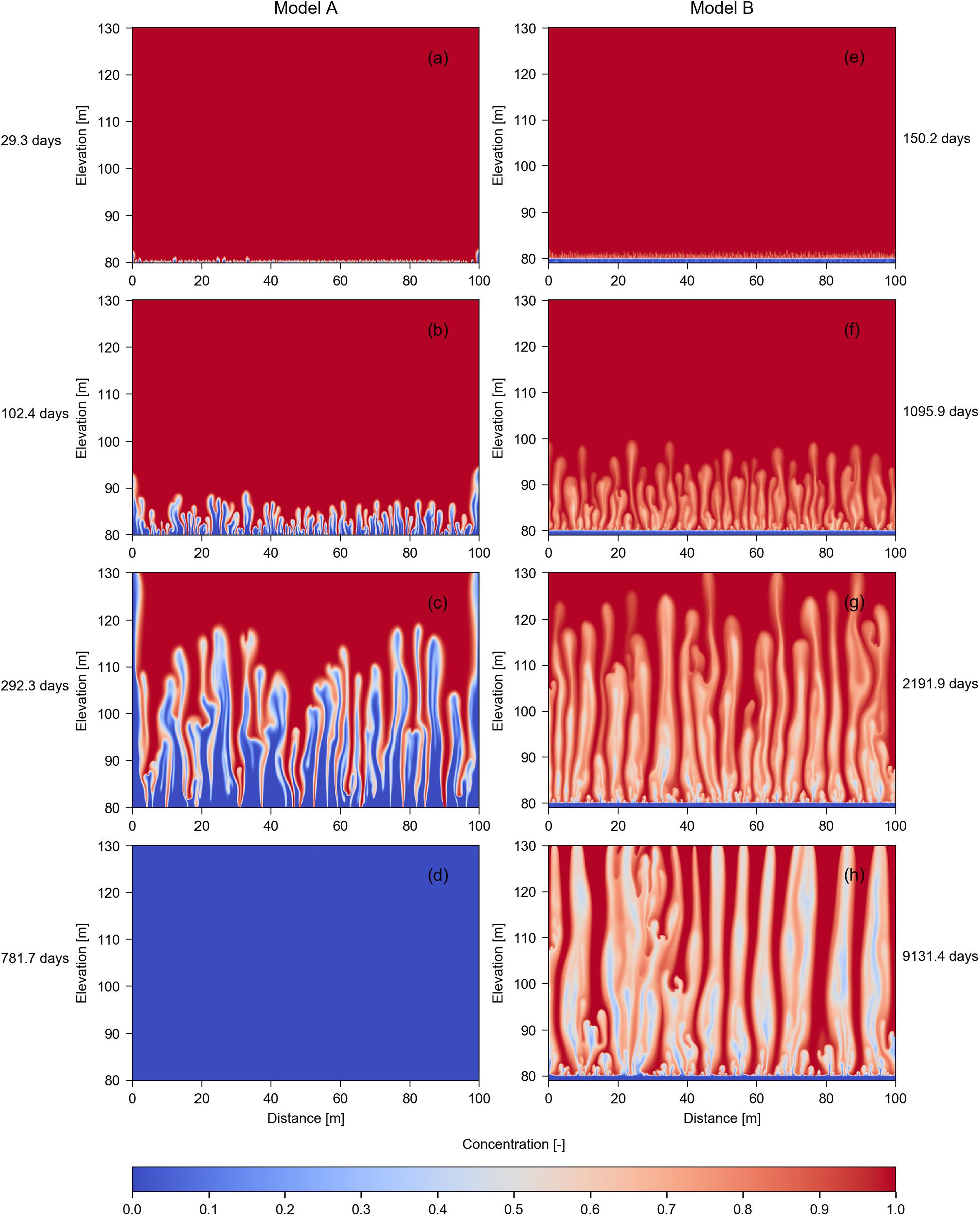
Figure 3. Salinity distributions in seafloor sediments obtained from simulations of the Base Case (i.e., α_L = 0.1 m; α_T = 0.01 m) of Model A (left column) and Model B (right column) at various simulation times. Concentration values represent the relative seawater concentration, where 0 and 1 are freshwater and seawater, respectively. The bottom left subplot depicts steady state results, while the bottom right subplot shows a quasi-steady state salinity distribution. (a) 29.3 days; (b) 102.4 days; (c) 292.3 days; (d) 781.7 days; (e) 150.2 days; (f) 1095.9 days; (g) 2191.9 days; (h) 9131.4 days.

FIGURE 4

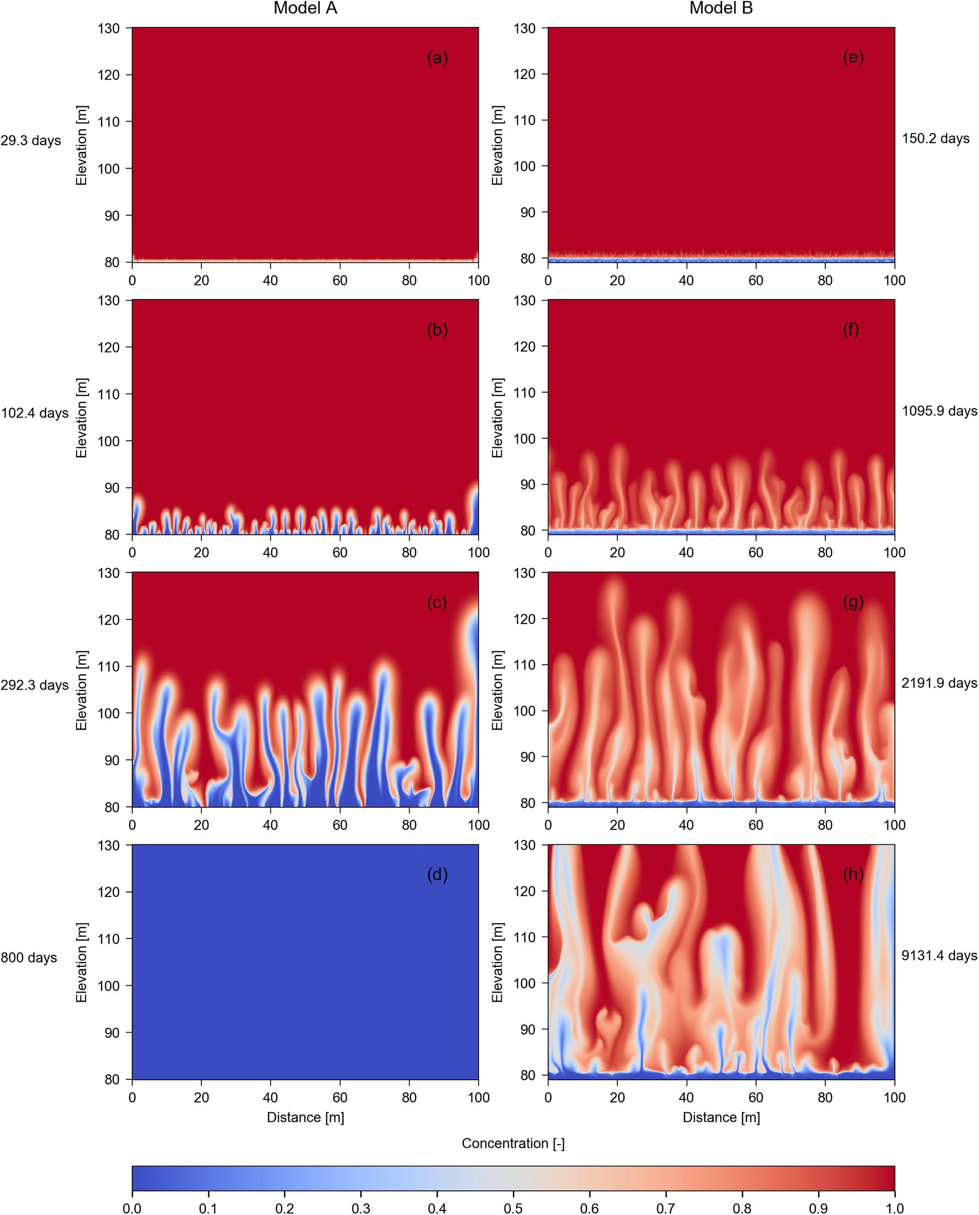
Figure 4. Salinity distributions in seafloor sediments obtained from simulations of Case 1 (i.e., α_L = 0.5 m; α_T = 0.05 m) of Model A (left column) and Model B (right column) at various simulation times. Concentration values represent the relative seawater concentration, where 0 and 1 are freshwater and seawater, respectively. The bottom left subplot depicts steady-state results, while the bottom right subplot shows a quasi-steady state salinity distribution. (a) 29.3 days; (b) 102.4 days; (c) 292.3 days; (d) 800 days; (e) 150.2 days; (f) 1095.9 days; (g) 2191.9 days; (h) 9131.4 days.

FIGURE 5

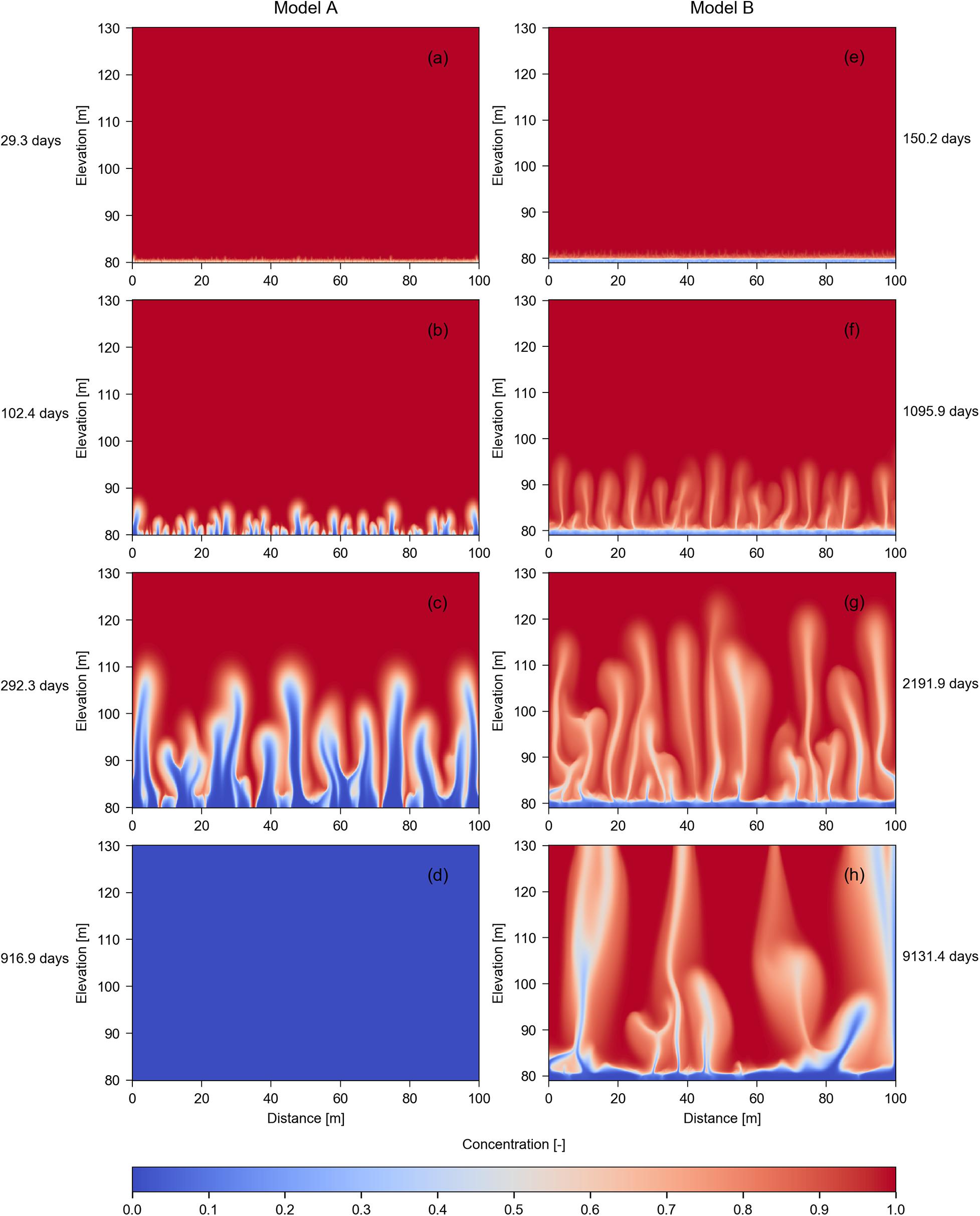
Figure 5. Salinity distribution in seafloor sediments obtained from simulations of Case 2 (i.e., α_L = 1 m; α_T = 0.1 m) of Model A (left column) and Model B (right column) at various simulation times. Concentration values represent the relative seawater concentration, where 0 and 1 are freshwater and seawater, respectively. The bottom left subplot depicts steady-state results, while the bottom right subplot shows a quasi-steady state salinity distribution. (a) 29.3 days; (b) 102.4 days; (c) 292.3 days; (d) 916.9 days; (e) 150.2 days; (f) 1095.9 days; (g) 2191.9 days; (h) 9131.4 days.

Figures 3–5 highlight substantial differences in mixed-convective processes caused by the existence (or not) of a leaky aquitard below the subsea aquifer. The most important difference between Models A and B, in the context of SFGD characteristics, is that unstable solute patterns persist under quasi-steady state in Model B, whereas in Model A, the flow instabilities are temporary, and the system reaches a steady state condition in which the aquifer is completely fresh. The occurrence of the leaky aquitard creates other important differences in mixed convective processes. For example, freshwater fingers produced from Model A are fresher, for fingers of a comparable height, to those produced by Model B (e.g., Figures 3c,g). This leads to sharper freshwater-saltwater interfaces in Model A results. The timescales for the rise of buoyant fingers also differ between Models A and B. For example, the time to obtain freshwater fingers of a roughly similar height differs substantially, as evident in the timing of 292.3 days for Figure 4c (Model A) and 2191.9 days for Figure 4g (Model B). Thus, the lower aquitard in Model B significantly restricts finger speeds, which is an intuitive outcome. HBF in Model A for the Base Case, Case 1, and Case 2 reaches elevations of 119.15, 110.95, and 110.75 m in Figures 3c, 4c, 5c, respectively. These represent average finger speeds of 48.9, 38.7, and 38.4 m/year. Lower velocities are produced in all three cases of Model B. That is, HBF heights were 129.85, 127.15, and 120.95 m in Figures 3g, 4g, 5g, leading to velocities of 8.31, 7.86, and 6.82 m/year, respectively. There is evidence of boundary effects in Model A, associated with the vertical no-flow boundaries, that was also observed by Xie et al. (2011). Greater velocities of fingers adjacent to no-flow boundaries are attributed to the absence of the host fluid (i.e., seawater) moving in the opposite direction to the buoyant fingers, which is otherwise expected to retard the finger upwelling speed. For that reason, fingers adjacent to vertical boundaries were neglected in assessing HBF speeds.

According to Xie et al. (2011), the theoretical velocity of fingers is 13.1 m/year, based on (△ρK/ρ_fε)×f, where f (0.115) is the Xie et al. (2011) corrective factor to the theoretical convective velocity (i.e., the ratio between Equation 7 and ε). Interestingly, the Xie et al. (2011) corrected convective velocity, which neglects the leaky layer in Model B, is closer to the results in Model B (i.e., 8.31, 7.86, and 6.82 m/year), compared to the finger velocities in Model A (i.e., 48.9, 38.7, and 38.4 m/year). However, finger velocities in Model A could be better predicted applying values of f that fall within the range of corrective factors proposed by Post and Kooi (2003) and Wooding (1969) (i.e., 0.22 and 0.446, respectively).

Figure 6 illustrates the temporal variability in total solute mass within model domains, for the six scenarios considered in this study. The fluctuations in total mass in Model B are caused by mixed-convective instabilities, which persist as quasi-steady state conditions, as discussed above. The time for Model A to reach steady-state conditions (approximately 2 years) is much less than the time required for Model B to reach quasi-steady state conditions (approximately 10 years). This is consistent with the difference between buoyant fingering speeds found in Models A and B, as discussed above. The larger velocities in Model A (e.g., 48.9 m/year, 38.7 m/year, and 38.4 m/d in Figures 3c, 4c, 5c) led shorter timescales to reach steady state compared to Model B, in which velocities were 8.31, 7.86, and 6.82 m/year (Figures 3g, 4g, 5g).

FIGURE 6

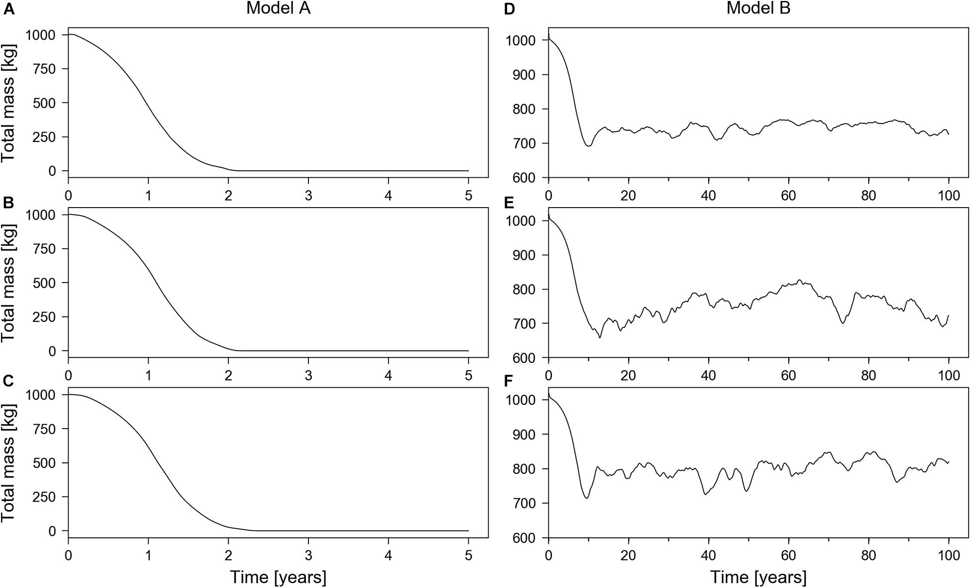
Figure 6. Numerical model results of total solute mass with time. (A,D) Base Case (i.e., α_L = 0.1 m; α_T = 0.01 m); (B,E) Case 1 (i.e., α_L = 0.5 m; α_T = 0.05 m); and (C,F) Case 2 (i.e., α_L = 1 m; α_T = 0.1 m). The left column represents cases of Model A and the right column represents cases of Model B.

The Influence of Dispersion

Figure 6 shows that variations in dispersion had no noticeable impact on the time required to reach steady and quasi-steady state conditions. This is consistent with the relatively small change between cases (i.e., from Base Case to Case 2) in buoyant fingering speeds, as observed also by Xie et al. (2011). The little influence of dispersion on buoyant fingering speeds is also in accordance with the definition of the theoretical convective velocity proposed by Xie et al. (2011), which neglects dispersion. While dispersion has an unimportant role in the speed of buoyant finger rise, dispersion does appear to influence the quasi-steady state buoyant fingering patterns associated with mixed-convective processes (Figures 3–5).

Figure 7 compares the three cases (i.e., Base Case, Case 1, and Case 2) of Model B, showing quasi-steady state salinity distributions in profile, and the temporal variation in SFGD solute concentration at the seafloor using a timeframe of 85 years. Subplots Figures 7a–c correspond to Figures 3h, 4h, 5h, respectively.

FIGURE 7

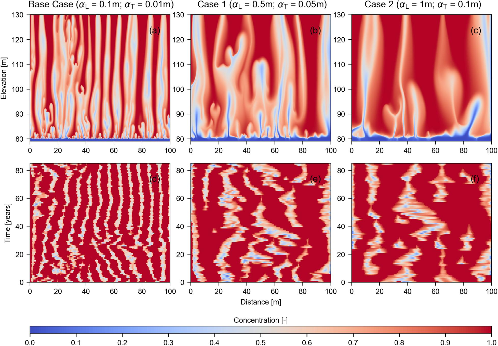
Figure 7. Salinity distribution in profile [subplots (a–c); top row] and temporal variation of solute concentration [subplots (d–f); bottom row] in seafloor sediments obtained from Model B simulations: Subplots are (from left to right) the Base Case, Case 1, and Case 2. Concentration values represent the relative seawater concentration, where 0 and 1 are freshwater and seawater, respectively. All subplots show a quasi-steady state salinity distribution.

Figure 7 shows that the number of fingers reaching the seafloor decreases with increasing dispersion due to the widening of fingers_; a similar observation to those of Xie et al. (2011) for dense, downward-moving fingers.

The temporal and spatial variability in the salinity distribution across the sea floor have important implications for the direct measurement of SFGD. For example, the deployment and size of seepage meters (e.g., Burnett et al., 2006) in areas where mixed-convective processes occur require consideration of the spatial variability in freshwater discharge, given the irregular distributions of SFGD in Figures 3–7. Mixed-convective flow leads to regions of freshwater upwelling and seawater downwelling, and therefore, SFGD measurement methods that can detect seafloor fluxes in both directions (inflow and outflow) may assist in detecting mixed-convective phenomena. Additionally, the duration of seepage meter placement should consider the temporal variation of SFGD created by mixed convective processes. Freshwater upwelling appeared to be relatively stable over durations of days-to-weeks, but may vary substantially over longer timeframes, at least for the cases illustrated in Figure 7.

The non-dimensional parameters Ra and M were determined, using Equations 1 and 5, respectively, from the quasi-steady state results of Model B. The steady-state solution of Model A has no density gradients within the aquifer (i.e., the aquifer is freshwater-filled), and therefore, both Ra and M (and Ra_δ) are zero. Given that the system is forced-convection dominated, SFGD to the seafloor under the Model A conditions will be diffusive or uniformly distributed.

For the application of Equation 5 to estimate M for Model B, an average q_z (across the bottom aquifer) over about 85 years of quasi-steady state conditions was used, based on the numerical results. The need to know q_z in applying Equation 5 to estimate M (or Ra_δ), as a predictor of buoyancy-driven flow, is potentially problematic for the purposes of designing SFGD monitoring systems (e.g., deployment of seepage meters), because rates of SFGD are typically not known prior to seepage meter deployment. For example, Stevens et al. (2009) estimated M by applying Equation 4, which requires the vertical hydraulic gradient (based on localized measurements of hydraulic heads and salinities from bore data) rather than q_z. Nevertheless, where mixed convective processes occur in seafloor sediments, the vertical hydraulic gradient is also difficult to ascertain considering the changes in location and temporal variations of SFGD caused by buoyancy forces. Alternative approaches to estimating q_z, such as the application of geochemical tracers (e.g., Taniguchi et al., 2019), may overcome difficulties in measuring hydrogeological variables within seafloor sediments.

The steady-state value of q_z is 2.9 × 10^–3 m/d in the Base Case (Figure 7a), 2.9 × 10^–3 m/d in Case 1 (Figure 7b), and 2.3 × 10^–3 m/d in Case 2 (Figure 7c). While the values of M for the three cases of Model B vary within the same order of magnitude (i.e., 22–27), the range of values of Ra is wider (i.e., 2031, 431, and 264 for the Base Case, Case1, and Case 2, respectively). These values indicate that the flow system in Model B is free-convection dominated. That is, M > 1, and the critical values of Ra_δ (or M) and Ra (i.e., 10 and 5, respectively) are also exceeded, indicating that unstable solute motion is likely to occur. Therefore, the occurrence of unstable flow in the current cases are consistent with critical values proposed in the literature for downwards salinization (e.g., Wooding et al., 1997; Smith and Turner, 2001). However, further investigation is warranted to ascertain if those critical values can be generally applied to SFGD through sandy seafloor sediments.

Conclusion

This research highlights that the occurrence of SFGD in permeable seafloor sediments potentially involves unstable flow processes, with important implications for SFGD measurement and the understanding of seafloor ecosystems. This study provides insight into SFGD measurement approaches, since we have demonstrated that for the cases considered here, SFGD measurements through the deployment of seepage meters will depend on the placement and measurement duration of seepage meters. Predicting whether unstable flow processes occur is theoretically plausible based on our overview of the most common non-dimensional numbers (i.e., Ra_δ, Ra, and M) used previously to characterize mixed-convection processes in groundwater. Simplified numerical models that represent submarine aquifers settings show that SFGD can occur in the form of upward freshwater fingers, analogous to the inverse downward movement of dense solute fingers. We found that the critical values of Ra_δ and Ra proposed in the literature for solute convection apply to the two cases analyzed in this study, although, further investigation is needed to generalize the use of those critical values to SFGD through sandy seafloor sediments. That is, further research into SFGD through high-permeability sediments is warranted to constrain the application of non-dimensional numbers for predicting unstable conditions, given the substantial differences between stable and unstable salinity patterns and distributions of SFGD to the seafloor. The results of this study show that the pattern of SFGD through high-permeability sediments containing seawater is controlled by the lower boundary, intended to represent either an underlying aquifer or aquitard. The numerical results also showed quasi-steady temporal fluctuations in the SFGD pattern behavior, for the case involving a low-permeability layer beneath the seafloor aquifer.

Data Availability Statement

The raw data supporting the conclusions of this article will be made available by the authors, without undue reservation.

Author Contributions

SS-R: numerical modeling, investigation, analysis, visualization, and writing – original draft and editing. AW: conceptualization, supervision, visualization, and writing – review and editing. DI: supervision, visualization, and writing – review and editing. All authors contributed to the article and approved the submitted version.

Funding

SS-R was supported by a Research Training Program scholarship. AW was the recipient of an Australian Research Council Future Fellowship (project number FT150100403).

Conflict of Interest

The authors declare that the research was conducted in the absence of any commercial or financial relationships that could be construed as a potential conflict of interest.

References

Bakker, M., Miller, A. D., Morgan, L. K., and Werner, A. D. (2017). Evaluation of analytic solutions for steady interface flow where the aquifer extends below the sea. J. Hydrol. 551, 660–664. doi: 10.1016/j.jhydrol.2017.04.009

CrossRef Full Text | Google Scholar

Burnett, W. C., Aggarwal, P. K., Aureli, A., Bokuniewicz, H., Cable, J. E., Charette, M. A., et al. (2006). Quantifying submarine groundwater discharge in the coastal zone via multiple methods. Sci. Total Environ. 367, 498–543. doi: 10.1016/j.scitotenv.2006.05.009

PubMed Abstract | CrossRef Full Text | Google Scholar

Elder, J. W., Simmons, C. T., Diersch, H., Frolkoviè, P., Holzbecher, E., and Johannsen, K. (2017). The elder problem. Fluids 2:11. doi: 10.3390/fluids2010011

CrossRef Full Text | Google Scholar

Guo, W., and Langevin, C. D. (2002). User’s Guide to SEAWAT: A Computer Program for the Simulation of Three-Dimensional Variable-Density Ground-Water Flow: Techniques of Water-Resources Investigations of the U. S. Geological Survey. Book 6, Chapter A7, Open File, 01-434. Tallahassee: US Geological Survey, 77.

Google Scholar

Irvine, D. J., Sheldon, H. A., Simmons, C. T., Werner, A. D., and Griffiths, C. M. (2015). Investigating the influence of aquifer heterogeneity on the potential for thermal free convection in the Yarragadee Aquifer, Western Australia. Hydrogeol. J. 23, 161–173. doi: 10.1007/s10040-014-1194-1

CrossRef Full Text | Google Scholar

Irvine, D. J., Werner, A. D., Ye, Y., and Jazayeri, A. (2021). Upstream dispersion in solute transport models: a simple evaluation and reduction methodology. Groundwater 59, 287–291. doi: 10.1111/gwat.13036

PubMed Abstract | CrossRef Full Text | Google Scholar

Jiao, J. J., Shi, L., Kuang, X., Lee, C. M., Yim, W. W. S., and Yang, S. (2015). Reconstructed chloride concentration profiles below the seabed in Hong Kong (China) and their implications for offshore groundwater resources. Hydrogeol. J. 23, 277–286. doi: 10.1007/s10040-014-1201-6

CrossRef Full Text | Google Scholar

Johannes, R. E. (1980). The ecological significance of the submarine discharge of groundwater. Mar. Ecol. Prog. Ser. 3, 365–373.

Google Scholar

Knight, A. C., Werner, A. D., and Morgan, L. K. (2018). The onshore influence of offshore fresh groundwater. J. Hydrol. 561, 724–736. doi: 10.1016/j.jhydrol.2018.03.028

CrossRef Full Text | Google Scholar

Kooi, H., and Groen, J. (2001). Offshore continuation of coastal groundwater systems; predictions using sharp-interface approximations and variable-density flow modelling. J. Hydrol. 246, 19–35. doi: 10.1016/S0022-1694(01)00354-7

CrossRef Full Text | Google Scholar

Kurylyk, B. L., Irvine, D. J., Mohammed, A. A., Bense, V. F., Briggs, M. A., Loder, J. W., et al. (2018). Rethinking the use of seabed sediment temperature profiles to trace submarine groundwater flow. Water Resour. Res. 54, 4595–4614. doi: 10.1029/2017WR022353

CrossRef Full Text | Google Scholar

Langevin, C. D., Thorne, D. T. Jr., Dausman, A. M., Sukop, M. C., and Guo, W. (2008). SEAWAT Version 4: A Computer Program for Simulation of Multi-Species Solute and Heat Transport. U.S. Geological Survey Techniques and Methods. Book 6, Chap. A22. Reston: US Geological Survey, 39.

Google Scholar

Lapwood, E. R. (1948). Convection of a fluid in a porous medium. Math. Proc. Cambridge Philos. Soc. 44, 508–521. doi: 10.1017/S030500410002452X

CrossRef Full Text | Google Scholar

Michael, H. A., Mulligan, A. E., and Harvey, C. F. (2005). Seasonal oscillations in water exchange between aquifers and the coastal ocean. Nature 436, 1145–1148. doi: 10.1038/nature03935

PubMed Abstract | CrossRef Full Text | Google Scholar

Michael, H. A., Scott, K. C., Koneshloo, M., Yu, X., Khan, M. R., and Li, K. (2016). Geologic influence on groundwater salinity drives large seawater circulation through the continental shelf. Geophys. Res. Lett. 43, 10782–10791. doi: 10.1002/2016GL070863

CrossRef Full Text | Google Scholar

Moore, W. S. (1999). The subterranean estuary: a reaction zone of ground water and sea water. Mar. Chem. 65, 111–125. doi: 10.1016/S0304-4203(99)00014-6

CrossRef Full Text | Google Scholar

Moore, W. S., and Wilson, A. M. (2005). Advective flow through the upper continental shelf driven by storms, buoyancy, and submarine groundwater discharge. Earth Planet. Sci. Lett. 235, 564–576. doi: 10.1016/j.epsl.2005.04.043

CrossRef Full Text | Google Scholar

Post, V., Kooi, H., and Simmons, C. (2007). Using hydraulic head measurements in variable-density ground water flow analyses. Groundwater 45, 664–671. doi: 10.1111/j.1745-6584.2007.00339.x

PubMed Abstract | CrossRef Full Text | Google Scholar

Post, V. E. A., and Kooi, H. (2003). Rates of salinization by free convection in high-permeability sediments: insights from numerical modeling and application to the dutch coastal area. Hydrogeol. J. 11, 549–559. doi: 10.1007/s10040-003-0271-7

CrossRef Full Text | Google Scholar

Riedl, R. J., Huang, N., and Machan, R. (1972). The subtidal pump: a mechanism of interstitial water exchange by wave action. Mar. Biol. 13, 210–221. doi: 10.1007/BF00391379

CrossRef Full Text | Google Scholar

Simmons, C. T., and Narayan, K. A. (1997). Mixed convection processes below a saline disposal basin. J. Hydrol. 194, 263–285. doi: 10.1016/S0022-1694(96)03204-0

CrossRef Full Text | Google Scholar

Simmons, C. T., Bauer-Gottwein, P., Graf, T., Kinzelbach, W., Kooi, H., Li, L., et al. (2010). “Variable density groundwater flow: from modelling to applications,” in Groundwater Modelling in Arid and Semi-Arid Areas, eds H. Wheater, S. A. Mathias, and X. Li (Cambridge: Cambridge University Press), 87–118.

Google Scholar

Smith, A. J. (2004). Mixed convection and density-dependent seawater circulation in coastal aquifers. Water Resour. Res. 40:W08309. doi: 10.1029/2003WR002977

CrossRef Full Text | Google Scholar

Smith, A. J., and Turner, J. V. (2001). Density-dependent surface water-groundwater interaction and nutrient discharge in the swan – canning estuary. Hydrol. Process. 15, 2595–2616. doi: 10.1002/hyp.303

CrossRef Full Text | Google Scholar

Solórzano-Rivas, S. C., and Werner, A. D. (2018). On the representation of subsea aquitards in models of offshore fresh groundwater. Adv. Water Resour. 112, 283–294. doi: 10.1016/j.advwatres.2017.11.025

CrossRef Full Text | Google Scholar

Solórzano-Rivas, S. C., Werner, A. D., and Irvine, D. J. (2019). Dispersion effects on the freshwater–seawater interface in subsea aquifers. Adv. Water Resour. 130, 184–197. doi: 10.1016/j.advwatres.2019.05.022

CrossRef Full Text | Google Scholar

Stevens, J. D., Sharp, J. M. Jr., Simmons, C. T., and Fenstemaker, T. R. (2009). Evidence of free convection in groundwater: field-based measurements beneath wind-tidal flats. J. Hydrol. 375, 394–409. doi: 10.1016/j.jhydrol.2009.06.035

CrossRef Full Text | Google Scholar

Taniguchi, M., Burnett, W. C., Smith, C. F., Paulsen, R. J., O’Rourke, D., Krupa, S. L., et al. (2003). Spatial and temporal distributions of submarine groundwater discharge rates obtained from various types of seepage meters at a site in the Northeastern Gulf of Mexico. Biogeochemistry 66, 35–53. doi: 10.1023/B:BIOG.0000006090.25949.8d

CrossRef Full Text | Google Scholar

Taniguchi, M., Dulai, H., Burnett, K. M., Santos, I. R., Sugimoto, R., Stieglitz, T., et al. (2019). Submarine groundwater discharge: updates on its measurement techniques, geophysical drivers, magnitudes, and effects. Front. Environ. Sci. 7:141. doi: 10.3389/fenvs.2019.00141

CrossRef Full Text | Google Scholar

van Reeuwijk, M., Mathias, S. A., Simmons, C. T., and Ward, J. D. (2009). Insights from a pseudospectral approach to the elder problem. Water Resour. Res. 45:W04416. doi: 10.1029/2008WR007421

CrossRef Full Text | Google Scholar

Voss, C. I., and Souza, W. R. (1987). Variable density flow and solute transport simulation of regional aquifers containing a narrow freshwater−saltwater transition zone. Water Resour. Res. 23, 1851–1866. doi: 10.1029/WR023i010p01851

CrossRef Full Text | Google Scholar

Webster, I. T., Norquay, S. J., Ross, F. C., and Wooding, R. A. (1996). Solute exchange by convection within estuarine sediments. Estuar. Coast. Shelf Sci. 42, 171–183. doi: 10.1006/ecss.1996.0013

CrossRef Full Text | Google Scholar

Werner, A. D., and Robinson, N. I. (2018). Revisiting analytical solutions for steady interface flow in subsea aquifers: aquitard salinity effects. Adv. Water Resour. 116, 117–126. doi: 10.1016/j.advwatres.2018.01.002

CrossRef Full Text | Google Scholar

Wooding, R. A. (1969). Growth of fingers at an unstable diffusing interface in a porous medium or Hele-Shaw cell. J. Fluid Mech. 39, 477–495. doi: 10.1017/S002211206900228X

CrossRef Full Text | Google Scholar

Wooding, R. A., Tyler, S. W., and White, I. (1997). Convection in groundwater below an evaporating salt lake: 1. Onset of instability. Water Resour. Res. 33, 1199–1217. doi: 10.1029/96WR03533

CrossRef Full Text | Google Scholar

Xie, Y., Simmons, C. T., and Werner, A. D. (2011). Speed of free convective fingering in porous media. Water Resour. Res. 47:W11501. doi: 10.1029/2011WR010555

CrossRef Full Text | Google Scholar

Xie, Y., Simmons, C. T., Werner, A. D., and Ward, J. D. (2010). Effect of transient solute loading on free convection in porous media. Water Resour. Res. 46, 389–400. doi: 10.1029/2010WR009314

CrossRef Full Text | Google Scholar

Zech, A., Attinger, S., Cvetkovic, V., Dagan, G., Dietrich, P., Fiori, A., et al. (2015). Is unique scaling of aquifer macrodispersivity supported by field data? Water Resour. Res. 51, 7662–7679. doi: 10.1002/2015WR017220

CrossRef Full Text | Google Scholar