Assessment of Aeolian Activity in the Bodélé Depression, Chad: A Dense Spatiotemporal Time Series From Landsat-8 and Sentinel-2 Data

1 Introduction

In areas that lack vegetation cover and water resources and exhibit low soil fertility, low rainfall, high temperatures, high evaporation levels, and high sand availability, effective wind plays a crucial role in aeolian processes. In several desert areas, the instability of dunes and sand sheets poses an important threat to transportation networks, water supply routes, urban areas, cultural sites, and human activities (Middleton and Sternberg, 2013; Ahmady-Birgani et al., 2017; Ding et al., 2020a). Monitoring dune migrations in spatiotemporal domains contributes to a deeper understanding of the aeolian process and its relationship with environmental changes (Hugenholtz et al., 2012). Moreover, information on dune migration can be used as an indicator of the presence or absence of large-scale trends in windiness over major deserts (e.g., the Sahara Desert), and these wind trends may influence the global dust budget (Vermeesch and Leprince, 2012).

Observations with high spatiotemporal resolution are required to decipher the complex patterns of dune migration (Hugenholtz et al., 2012). Ground-based measurements offer higher accuracy but provide sparse coverage in spatiotemporal domains. The development of remote sensing techniques, including optical and radar imagery and digital elevation models (DEMs), allows the investigation of geomorphological changes with dense spatiotemporal measurements. The majority of studies addressing the evolution of dune dynamics have been conducted using optical imagery (Manzoni et al., 2021). Compared to the optical imageries, the dependency on synthetic-aperture radar (SAR) imagery to monitor dune migration is not extensive. Previous studies that employed SAR imagery (e.g., Rozenstein et al., 2016; Gaber et al., 2018; Ullmann et al., 2019; Manzoni et al., 2021) mainly depended on interferometric coherence as an indicator of dune and sand sheet instability. Notably, these coherence-based techniques do not provide any quantitative representation of dune dynamics, however, can be used as a proxy for the fine movements of dunes and sand sheets. Several approaches to optical imagery have been used to capture information about dune dynamics at various resolutions, including classical methods and visual interpretation (e.g., Hereher, 2010; Hamdan et al., 2016), GIS strategies (e.g., Ghadiry et al., 2012; El-magd et al., 2013), and optical image cross-correlation (OICC) (e.g., Vermeesch and Drake, 2008; Hermas et al., 2012; Scheidt and Lancaster, 2013; Sam et al., 2015; Ali et al., 2021).

With the rapid development of OICC, mapping the surface displacement of large areas at very high spatiotemporal resolution is now feasible and reliable (Stumpf et al., 2016). Various types of data were used to perform such correlations, including optical and SAR images and DEMs. Optical images were the most commonly used due to the availability of free archives (Dille et al., 2021). Co-registration of optical image matching and correlation (COSI-Corr) (Leprince et al., 2007) is considered the most widely used method for retrieving surface deformations due to its excellent performance in terms of processing time, output variables, and provision of multiple pre- and post-processing modules (Jawak et al., 2018). COSI-Corr has been used to monitor various targets, including earthquakes (e.g., Ayoub et al., 2009; Avouac et al., 2014; Chen et al., 2020), landslides (e.g., Stumpf et al., 2014; Lacroix et al., 2019; Yang et al., 2021), glaciers (e.g., Scherler et al., 2008; Shukla and Garg, 2020; Das and Sharma, 2021), and dunes (e.g., Necsoiu et al., 2009; Vermeesch and Leprince, 2012; Hermas et al., 2019). OICC provides subpixel measurements of surface deformations with an accuracy of up to a tenth of the ground resolution (Leprince et al., 2007).

TSI-OICC measurements has recently been used to monitor the temporal evolution of various targets, including landslides (e.g., Bontemps et al., 2018; Lacroix et al., 2019; Dille et al., 2021; Ding et al., 2021), glaciers (Altena et al., 2019), and dunes (e.g., Ali et al., 2020; Ding et al., 2020a; Ding et al., 2020b). Bontemps et al. (2018) were the first to construct a complete network of matching pairs from 16 SPOT–5 images covering 35 years and inverted it to monitor landslide deformations. Large differences in solar angles affected the matching results, leading to seasonal signals, while large temporal separation affected the temporal decorrelation (Bontemps et al., 2018; Lacroix et al., 2019). The inversion of the full network is promising for controlling uncertainties and improving spatial coverage; however, generating full networks from the available free archives [i.e., Landsat-8 (L-8) and Sentinel-2 (S-2)] would increase the computational cost and data burden. Recently, some studies (e.g., Ali et al., 2020; Ding et al., 2020b; Ding et al., 2021) have simulated small baseline subset (SBAS) approaches used in InSAR for application in the optical image matching domain, selecting only pairs with certain baseline thresholds. SBAS-based optical image matching mainly aims to reduce computation times and data burdens (Bui et al., 2020) and improve the quality of pairs by limiting probable cast shadows, while achieving higher spatial coverage with lower uncertainty. The presented SBAS-based optical image matching approach has shown potential for capturing the temporal patterns of various targets, including dunes (Ding et al., 2020a; Ali et al., 2020; Ding et al., 2020b) and landslides (Ding et al., 2021), with low uncertainty and high spatial coverage.

The Bodélé depression (BD) in Chad is a 133,532 km² elongated paleolake that is gaining importance as a global source of mineral dust and a natural aeolian laboratory because it is considered the dustiest place on the Earth (Bristow et al., 2009). Barchan dunes are the predominant dune morphology in the BD, but their geochemical formation differs between the center and the margins of the BD (Hudson-Edwards et al., 2014). The crust of the Barchan dunes inside the depression is composed of diatomite with a lower density than quartz, which is the major dune constituent along the margins of the depression. Accordingly, dune migration is faster in the center of the BD than elsewhere, and these Barchan dunes are considered the fastest worldwide (Bristow et al., 2009). The geomorphological formation of the dunes detected by the two L-8 frames varied between the two formations (see Figure 1B). The Barchan dunes in the BD, have been studied using OICC three times in the existing literature. Vermeesch and Drake (2008) first used COSI-Corr, along with ASTER images, to test the performance of the correlation as the temporal separation was adjusted. They reported the effect of temporal decorrelation in reducing the signal-to-noise ratio of the results. Vermeesch and Leprince (2012) matched seven adjacent optical images from different sensors to track dune migration over 26 years. They reported that variations in migration rates were up to 10%, equivalent to a 0.2% variation in wind speed per year, indicating stability in wind conditions. Recently, Baird et al. (2019) proposed a workflow to extract representative dune migration rates by feeding Landsat-5 data into the correlation engine.

FIGURE 1

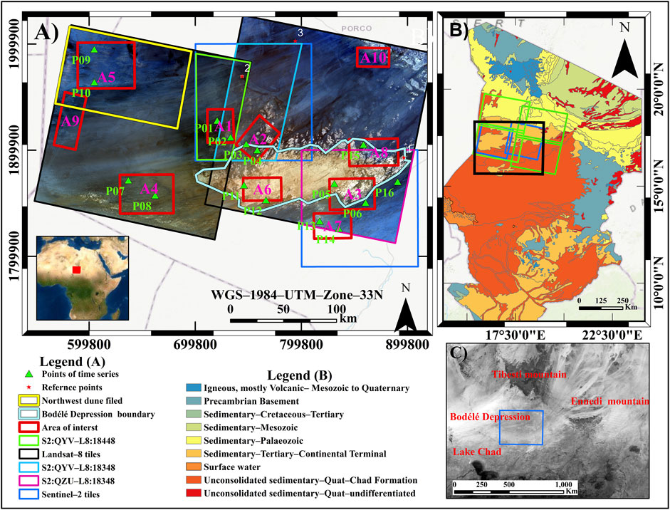
FIGURE 1. Geographical position and geological formation of the study area. Panel (A) indicates the location of the Bodélé Depression. The inset shows the location of the BD in Africa. The background in panel (A) is a mosaic of Landsat-8 false colors. The black rectangles denote the coverage of Landsat-8 (i.e., P:183/R:48 and P:184/R:48). The blue rectangles denote the coverage of Sentinel-2A/B (i.e., TR33QYV and TR33QZU). The red rectangles represent the dune fields for which we discuss the spatiotemporal variability in Section 4.6. The red pentagrams represent the reference points used for absolute calibration, while the green triangles represent the points for which we extracted the temporal evolution of dune migration in Section 4.5. The three colored polygons in panel (A) represent the overlap areas between Landsat-8 and Sentinel-2, where we performed the inversion of the fused offset maps. Panel (B) shows the geological and geomorphological formations of Chad. The black rectangle represents the area shown in panel (A). The green rectangles denote the Sentinel-1A coverage (i.e., descending tracks 07 and 80). Panel (C) shows the location of the BD in the gap between the Tibesti and Ennedi mountains, and the current coverage of Lake Chad to the southwest. The background is the MODIS surface reflectance.

From the existing literature, previous studies at BD have not provided a complete picture of the behavior of dune migration on short time scales (i.e., monthly, or weekly). Only the study by Vermeesch and Leprince (2012) produced long time series of matching measurements, using seven images covering the period from 1984–2010. The time-series presented did not provide information on the behavior of dune migration and associated wind patterns on a short time scale due to the sparse temporal samplings. Furthermore, the adjacent paring criterion of matching images to produce time series fails to provide high spatial coverage and low uncertainties. Moreover, monitoring the fast-moving targets requires matching images with short time separation, however, these short time spans would be affected by a large fraction of geolocation errors (Fahnestock et al., 2016). To best monitor the temporal evolution of dune migration with dense spatial and temporal coverage and low uncertainties, the application of optical image matching selection and inversion algorithm is feasible in monitoring the temporal evolution. The inversion algorithm first selects the appropriate images by constraining the cloud coverage. However, the number of available scenes (i.e., cloud-free) is primarily limited by cloud cover, especially during the rainy seasons prevalent in tropical regions, resulting in a reduction in temporal sampling. Therefore, the fusion of two or more sensors is considered feasible in providing a dense temporal sampling, to reveal the complex deformation patterns up to a weekly time scale. The main objectives of the study can be summarized as follows: 1) to broadly apply the time series selection algorithm from optical images and inversion to monitor the status of dune activity of the Bodélé Depression dunes with dense time series in the last decade (2013–2021), 2) to test the feasibility of merging the matching measurements from two sensors in condensing the time series and increasing the redundancy level, and 3) to study the spatiotemporal variability of dune migration in both seasonal and decadal changes. The rest of this study is organized as follows: the description of the geographical and geomorphological location and the data used are discussed in Section 2. Secondly, the methodology and rationale employed in this study are outlined in Section 3. Thirdly, the results and discussion of the temporal evolution of the Bodélé depression dunes are discussed in Section 4. After that, reflection on previous studies and the merit of the optical mage matching selection and inversion algorithm are investigated. At the end, the concluded remarks are summarized in Section 5.

2 Study Area and Datasets

2.1 Geological and Environmental Settings of the Bodélé Depression

There are several localized “hotspots” of dust production in the central Sahara, the most important being the BD in northern Chad (Goudie and Middleton, 2001; Chappell and Bristow, 2005). Historically, the BD hosted Lake Mega-Chad, which has now completely disappeared, exposing the lake sediments to deflation (Bristow et al., 2009). The BD is considered the largest source of aerosol dust worldwide; it is a 24,000 km² area that delivers about 6.5 million tons of Fe and 0.12 million tons of P to the Atlantic Ocean and Amazon Basin annually (Bristow et al., 2009). This can be explained by the following two factors: 1) A strong surface wind, known as the Bodélé low-level jet (LLJ), is directed at the BD (Washington et al., 2006). The location of the depression on the downwind side of the gap between the Tibesti and Ennedi Mountains on the border with Libya (Figure 1C) increases the leverage and activity of the northeast trade winds in the depression. 2) As a sub-basin of the Mega-Chad paleolake, the BD is a large source of erodible sediments, including lacustrine diatomaceous Earth (Washington et al., 2006; Warren et al., 2007). In addition, the area is a sparsely vegetated, hyper-arid region that provides extreme erodibility (Koren et al., 2006). The sediments produce white crusts of diatomaceous Earth that are easily mined and transported by the wind, forming some of the largest and fastest-moving Barchan dunes worldwide (Figure 1). There are two types of dunes in the area; the dunes at the edges of the depression are composed mainly of quartz, while those in the center contain diatomaceous Earth pellets. It is noteworthy that the central dunes have higher dune velocities than the marginal dunes because of their low density (Warren et al., 2007).

2.2 Datasets

2.2.1 Optical Images

We used satellite imagery from the free archives of L-8 and S-2 to feed into the COSI-Corr correlation engine to capture quantitative measurement of the dune migration up to 1/10 of pixel size (Leprince et al., 2007). The two sensors have similar characteristics in terms of their spectral properties and spatial and temporal resolutions (Roy et al., 2014; Kääb et al., 2016). We selected images with low cloud cover (less than 1%), and we have checked visually the images to avoid the selection of images contaminated by haze or dust, yielding a total of 168 images: 95 images obtained from two L-8 frames and 73 images from two S-2 tiles (Figure 1A). The temporal coverage of the L-8 and S-2 images is summarized in Figure 2, while Supplementary Tables S1–S4 provide an inventory of the metadata of the images. Both products are orthoimages with atmospheric correction of the reflectance values and geometric correction based on a refined geometric model. The processing chains of the L-8 products and S-2 data are considered identical in terms of the radiometric and geometric corrections, orthorectification, and resampling to a map grid (Roy et al., 2014; Kääb et al., 2016). We used the panchromatic (band 8) and NIR infrared band (8a) of S-2 to feed the correlation engine, according to the recommendations of Ali et al. (2020).

FIGURE 2

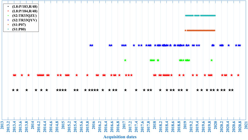
FIGURE 2. Temporal distribution of data used in the study. Landsat-8 frames (P:183/R:48) and (P:183/R:48) (43 and 52 scenes, respectively), Sentinel-2 tiles (TR33QYV and TR33QZU) (56 and 17 scenes, respectively), and Sentinel–1 descending orbits (07 and 80) (30 and 29 scenes, respectively). The cloud cover threshold for Sentinel-2 tile TR33QZU was set to 20% due to the cloud and dust. Detailed acquisition information is listed in Supplementary Tables S1–S5.

2.2.2 SAR Images

Radar imagery was used to determine the mobility of the sand dunes. In the dune environment, the phase from interferometric synthetic-aperture radar (InSAR) may not be suitable for tracking the rapid movement of sand dunes directly (i.e., 50 m/y). Alternatively, we used the metric of coherence, which represents the degree of similarity between repeat-pass observations, to map the stability of sand dunes (Wegmüeller et al., 2000; Ullmann et al., 2019). To provide an extensive spatial coverage and a stable revisit time (i.e., 12 days), we used two descending paths (Figure 1B) of Sentinel-1B data in 2019. Details of the images used for interferogram generation are presented in (Figure 2; Supplementary Table S5).

2.2.3 ECMWF/ERA Interim Metrological Data

We acquired the average monthly U and V wind components for each year from 2013 to 2021, measured in m/s with a resolution of 0.1 × 0.1 °, from the European Centre for Medium-Range Weather Forecasts (ECMWF) (Dee et al., 2011). The U and V components represent the eastward and northward components of the wind, respectively, at a height of 10 m above the surface of the Earth. The two components were combined to estimate the wind speed and direction. The average monthly wind speed and direction values for a selected region inside the BD for each year are displayed in Supplementary Figure S1. Also, we acquired the wind records for selected years (Supplementary Figure S1) from 1984 to 2007 to validate the comparison of dune velocities between the different decades in Section 4.5.4.

3 Methods

Figure 3 shows a flowchart outlining the main methodology and the structure of this article, including the following four main parts. In part 1, we used the Sentinel-1 imagery to delineate the stagnant regions by estimating the mean spatial coherence map (MSC) (see Section 3.1). We generated a network of interferograms from two descending tiles covering the study area during (Jan/2019-Dec/2019) and stacked the coherence maps to estimate the MSC to help define the stagnant regions. In Part 2, we applied optical image matching selection and the inversion algorithm to create a time series of dune movement from 2013–2021. The inversion algorithm involved several steps: Generation of a network of offset maps from the selected images, feature tracking of the selected pairs in the COSI-Corr environment, application of refinement steps to control the aberrant measurements, before the inversion of the time series we introduced the fusion between the offset maps of the two sensors, and post-processing of the inverted results. The fusion between time series was introduced to address the feasibility of the fusion in condensing the temporal coverage of time series especially when images are contaminated by large cloud cover. In part 3, we investigated the spatiotemporal variability of dune velocities in seasonal and decadal scales. In part 4, we compared the time series results from the inversion of each sensor individually and to the inversion of the fused time series. Additionally, we evaluated the performance of the inversion algorithm in controlling the uncertainties, whereas we compared the uncertainties of the individual offset maps before and after the inversion.

FIGURE 3

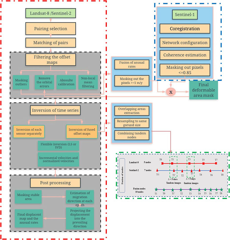
FIGURE 3. Flowchart of the processing chain. The steps outlined by the blue dashed rectangle represent the processing steps to estimate the multitemporal spatial coherence. The steps outlined by the red dashed rectangle denote the optical image matching selection and inversion algorithm. The green dashed rectangle denotes the concept of combining tandem images when merging data from the two sensors.

3.1 Multitemporal Spatial Coherence From SAR Images

Interferogram generation was performed by the InSAR Scientific Computing Environment (Agram et al., 2016). For each orbital path, we first generated a co-registered stack using geometrical co-registration and the enhanced spectral diversity method (Fattahi et al., 2017). We then removed the contribution of topography using the 1-arc Shuttle Radar Topography Mission DEM (Farr et al., 2007). We formed a network configuration that connected each image with two subsequent acquisitions. We did not filter the wrapped interferograms further to avoid potential contamination of the signal. The resultant interferograms were multi-looked using a 5 × 20 azimuth and range directions. From the resultant interferograms, we estimated the complex coherence, which represents the correlation between two SAR acquisitions (Touzi et al., 1999), as follows:

$\gamma =\frac{\left|{{\displaystyle \sum }}_{\mathit{k}=1}^{\mathit{N}}{\mathit{f}}_{\mathit{k}}{\mathit{g}}_{\mathit{k}}^{\mathrm{\star }}\right|}{\sqrt{{{\displaystyle \sum }}_{\mathit{K}=1}^{\mathit{N}}{\left|{\mathit{f}}_{\mathit{k}}\right|}^2{{\displaystyle \sum }}_{\mathit{K}=1}^{\mathit{N}}{\left|{\mathit{g}}_{\mathit{k}}\right|}^2}}(1)$

where $f_k$ and $g_k$ are the complex values from the primary and secondary SAR images surrounding the given pixel with window size $N$, and $f_k{g}_k^{\mathrm{\star }}$ is the complex conjugate operation for each interferogram. Using the coherence map stacks, the mean value of the spatial coherence ${\gamma }_{MSC}$ was estimated to delineate the spatial coherence in the study area, as follows:

${\mathit{\gamma }}_{\mathit{MSC}}\left(\mathit{i}\right)=\frac{1}{2\mathit{N}-3}{\displaystyle \sum }_{\mathit{n}=1}^{2\mathit{N}-3}\left|{\mathit{\gamma }}_{\mathit{n}}\left(\mathit{i}\right)\right|(2)$

where $i$ is the target pixel, $N$ is the total number of acquisitions, and ${\gamma }_n\left(i\right)$ is the coherence of the interferogram.

We used multitemporal spatial coherence (MSC) as a proxy for stagnant areas delineation, similar to the method used by Manzoni et al. (2021). The spatial distribution of the MSC is displayed in Supplementary Figure S2. The threshold used to define the stagnant areas in that study was set by trial and error, whereas we iteratively tested several threshold values from 0.70 to 0.90. The optimum threshold was selected to achieve the best match with the average annual magnitudes (AAMs) extracted from the inversion of one rate solution. AAMs were determined after removing outliers representing the linear velocity of the dunes. AAMs below 0.5 m/y were assumed to be stagnant. The threshold MSC used to define stagnant areas was set iteratively to best match the lower values of the AMMs. Practically, we set the threshold of the MSC to 0.85 to define the stagnant areas. The spatial distribution of the active and stagnant areas is displayed in Supplementary Figure S3.

3.2 Optical Image Matching Selection and Inversion

3.2.1 Image Selection and Network Establishment

For the selected images $\left(N+1\right)$, a number of pairs can be generated that is between $N\le M\le \frac{N\left(N+1\right)}{2}$ (Berardino et al., 2002). In previous studies (Ali et al., 2020; Ding et al., 2020b), the baselines of the matching process (i.e., radiometric, temporal, and spatial baselines) were defined and weighted according to their effect on the measurement uncertainties as follows: Sun elevation difference, Sun angle difference, temporal baseline, and spatial baseline. We estimated the baselines for all possible pairing combinations and then set the thresholds to limit the choices. The thresholds were determined iteratively by considering their prior weights and preserving the network configuration (i.e., the connectivity of the established networks) (Reinisch et al., 2017). Increasing the maximum temporal baseline allows more pairs to be selected; however, it is recommended to limit the maximum temporal baseline to reduce surface changes and temporal decorrelations. We set the maximum temporal baseline to 6.5 and 3.5 years for L-8 and S-2, respectively, considering the nature of migration in the study area, and the selected window size. No limits were set for the shortest temporal baseline to promote good network connectivity. Short temporal separation values preserve surface changes and are necessary for monitoring fast targets; however, they are prone to large geolocation error effects (Fahnestock et al., 2016). Thus, we assigned a weighting criterion for the deformation maps based on their temporal separation (Section 3.2.5). After several trials, baseline thresholds were determined for both the L-8 and S-2 networks (Supplementary Table S6). Details of the baselines of all pairs are listed in Supplementary Tables S7–S13.

3.2.2 Optical Images-based Feature Tracking

The selected pairs were matched in the frequency domain of the correlation engine (COSI-Corr) (Leprince et al., 2007). Such correlations are generally performed in two steps: 1) a coarse estimation is provided using large sliding windows, and 2) subpixel accuracy is provided using smaller windows (Beaud et al., 2021). Three parameters were determined: the step size, which determines the spatial resolution of the displacement maps, and the initial and final window sizes. The optimal window size was selected after testing several window sizes and comparing the results in terms of the uncertainty of the stable targets. The parameters used to complete the matching process for L-8 and S-2 are summarized in Supplementary Table S6. These parameters were prepared in text files and fed into the batch processor of the correlation engine to decrease human intervention. The ground resolution of the deformation maps was unified as 60 m by setting step sizes of four and six pixels for L-8 and S-2, respectively. Each deformation map yielded displacement in the East–West (EW) and North–South (NS) directions, together with a signal-to-noise-ratio (SNR) map, which is considered a measure of correlation quality (Bontemps et al., 2018; Beaud et al., 2021).

3.2.3 Refinement of the Deformation Fields

Prior to the inversion of the offset maps, several filtering processes were applied to control the uncertainty and help capture real deformations (Figure 3): 1) The outliers were discarded. We estimated the yearly migration rates of all the deformation maps and pixels with $SNR\le 0.90$ and velocities $\ge 250 m/y$ were discarded from the EW and NS deformation maps. 2) Orbital noise was removed from the deformation fields. The orbital residual usually stems from the orthorectification and co-registration residuals (Ali and Xu, 2019; Ding et al., 2020b). Notably, the removal of such orbital errors generally requires the identification of stable ground. To better identify stable regions, we used a mask based on the MSC and AAMs (Section 3.1). After masking the deformable regions, polynomial surfaces were fitted and then removed from the raw deformations. 3) Absolute calibration of the deformation fields was conducted. Co-registration bias is assumed to be a uniform shift in both directions (i.e., EW and NS) over the entire deformation field (Friedl et al., 2021). We extracted a small stable area and estimated the median of the measurements, then corrected the deformation fields by adding or subtracting the determined medians (Friedl et al., 2021). 4) Non-local mean filtering was applied to the COSI-Corr environment to preserve the fine details of the correlation and control additive white noise (Shukla and Garg, 2020). This was achieved using the parameters summarized in Supplementary Table S6.

3.2.4 Preparation of the Fusion Between Two Sensors

The following points summarize the preparation of the fused deformation maps before inversion (see the green dashed rectangle in Figure 3): 1) The deformation maps of each sensor for the overlapping regions were extracted, resampled to a common geographic grid, and reordered chronologically. 2) The epochs from the two sensors were merged and reordered, and two epochs were considered tandem nodes (Usai, 2003) when the images were separated by less than 5 days. 3) Boundary adjustment was applied to account for variation in the temporal span owing to the merging process (Samsonov et al., 2020). The deformation maps were adjusted by multiplying the deformation values by the ratio between the new and old-time intervals. 4) The deformation maps, with identical start and end dates, were merged using median fusion (Samsonov et al., 2020).

3.2.5 Inversion of Displacement Time Series

We inverted the deformation maps associated with each sensor, and the overlapping zones between the two sensors, separately. We used the parameterization of Berardino et al. (2002) to construct the relationship between the displacement $d$ and the mean velocity between each adjacent epoch $v$ through design matrix $B$, according to Eq. 3. Design matrix $B$ is an $M\times N$ matrix, where each row contains the time increments between the master and slave of the pair (Berardino et al., 2002). The mean velocities between adjacent epochs can be obtained by inverting the matrix $\left(B^{\text{'}}PB\right)$ where $P$ is the weight of each deformation map. We performed the inversion using a pixel-wise strategy with a flexible design matrix B using either least-squares inversion (Usai, 2003), according to Eq. 4, or singular value decomposition, according to Eq. 5 (Berardino et al., 2002), based on the matrix condition (i.e., full rank or rank deficient). We restricted the inversion to pixels for which the stack size exceeded a certain threshold (75%) to strike a balance between ensuring good spatial coverage and reducing the oscillation of the singular value decomposition solution caused by a large number of subsets (Reinisch et al., 2017). We retrieved the pairs by back substitution after the first round of inversion, and then a second round of inversion was executed as per Bontemps et al. (2018). For the fusion between the two sensors, similar inversion procedures were applied. We determined the weight of each map according to the assumption that the error of the velocity reaches $0.1\times PS$ for a 1-year separation (Mouginot et al., 2017). Consequently, the velocity expression deteriorates, especially for short-time separations $TS$, according to Eq. 6 (Mouginot et al., 2017) (see Supplementary Table S14). Accordingly, we applied weighting criteria considering the precision of the estimated velocities. The estimated weights assigned for each time interval are listed in Supplementary Table S14.

$\mathit{Bv}=\mathit{d}(3)$

${\mathit{v}}_{\mathit{LS}}={\left({\mathit{B}}^{\prime }\mathit{PB}\right)}^{-1}{\mathit{B}}^{\prime }\mathit{Pd}(4)$

${\mathit{v}}_{\mathit{SVD}}=\mathit{V}{\mathit{S}}^{+}{\mathit{U}}^{\prime }{\mathit{B}}^{\prime }\mathit{Pd}(5)$

$ϵ=0.1\times \mathit{PS}\times \frac{365.25}{\mathit{TS}}(6)$

where the $U$ is an orthogonal matrix with dimension $M\times M$, including the eigenvector of matrix $B’PB$; the $S^{+}$ matrix is an $M\times M$ diagonal matrix including the singular values of ${\sigma }_i$; $V$ is a matrix with the dimensions of N × N including the eigenvectors of $\left(B^{\text{'}}PB\right)$; $\mathit{ϵ}$ is the velocity error; and $PS$ is the pixel ground resolution. The symbols ′ and $-1$ denote the transpose and the inverse of matrix, respectively.

3.3 Post-Processing

We converted the mean velocities between each adjacent epoch obtained by the inversion into cumulative displacement $D_m$ for both EW and NS, according to Eq. 7. The values were temporally related to the first scene (Supplementary Tables S1–S4) and spatially to the reference points (see Figure 1). The AAM and the corresponding prevailing migration direction (PMD) were estimated according to Eqs 8, 9, respectively. After acquiring the displacement, we applied the following refinement steps: 1) Masking pixels comes from the inversion of offset maps belonging to more than two subsets. 2) Masking non-active pixels using the stagnant mask obtained in previous steps. 3) Estimating the migration direction at each time stamp and then applying a median filter with a 3 × 3 window size. 4) Calculating the Euclidean norm representing the magnitudes. 5) Estimating the cumulative projected displacements (CPD) by projecting the displacement of each epoch in the PMD. The projection was performed by multiplying the magnitude of migration of each epoch by the cosine of the difference between the migration direction and the PMD.

${\mathit{D}}_{\mathit{m}}={\displaystyle \sum }_{\mathit{i}=2}^{\mathit{m}}{\mathit{v}}_{\mathit{i}}{\mathit{t}}_{\mathit{i}}(7)$

$\overline{\mathit{v}}={\left({\overline{\mathit{B}}}^{\prime }\mathit{P}\overline{\mathit{B}}\right)}^{-1}{\overline{\mathit{B}}}^{\prime }\mathit{Pd}(8)$

$\mathit{PMD}=\mathbf{atan}\left(\frac{\overline{\mathit{EW}}}{\overline{\mathit{NS}}}\right)(9)$

where $\overline{EW}$ and $\overline{NS}$ are linear velocity in the east-west and the north-south directions, respectively; $\overline{B}$ is a $M\times 1$ matrix includes the time separation between the master and slave images for each offset map and $\overline{v}$ is the AAM in m/yr.

3.4 Assessment of the Spatiotemporal Variability of Dune Migration

The BD exhibited large spatial variability in dune migration rates owing to the presence of different dune morphologies, chemical formations, and the interactions between wind speed and topography (Hudson-Edwards et al., 2014). To better capture the spatiotemporal variability of dune migration, we investigated four aspects as follows: 1) We compared the AAMs of the active aeolian features extracted from the L-8 solution with various dune fields spatially distributed across the study area (see Figure 1). For each selected dune field, we calculated the median, first and third quartiles, and interquartile range. We performed two significance tests (F-test and Welch’s two-sample test) to compare the extent to which the variance and mean of each dune field were significantly different compared to other dune fields, as described by Rouyet et al. (2019). Similarly, the tests were applied to assess the significance of the PMDs and MSCs. 2) To gain new insights into the variability of migration rates and direction, we used the redundancy of the offset maps and extracted the dune velocities (m/y) from all pairs. We then estimated the geometric mean of all active pixels associated with each dune field for each deformation map and extracted boxplots of each dune field representing the distribution of the geometric mean of the dune velocities between the different offset maps. The geometric mean was used rather than the normal mean to avoid overestimation as recommended by Baird et al. (2019). Similarly, we estimated the average migration direction and the corresponding concentration ratio (CR) of the active pixels associated with each dune field for all the deformation maps, according to Eqs 10, 11, respectively. We also drew a boxplot representing the variability of migration direction to examine the probable migration directions expected in the study area. 3) We examined the spatiotemporal variability of migration rates between different seasons from the inversion of the fused offset maps. We estimated the median velocity of the velocity values in similar seasons over the entire time series and estimated the seasonal sliding coefficients (SSC) representing the ratio of the median velocities between two seasons. 4) We examined the variability of dune velocities between different decades, by employing the matching between three Thematic Mapper images (17/01/1984, 1/12/1998, and 24/1/2007) to capture dune migration in two previous decades (see Table 1) and compare the results to our more recent rates (i.e., from 2013 to 2021). We mainly used the Thematic Mapper instead of the Enhanced Thematic Mapper due to the failure of Scan Line Corrector (SLC) after May 2003. We used band 4) of the Thematic Mapper sensor to fed into the correlation engine as per Baird et al. (2019).

$\overline{\mathit{\theta }}=\mathit{atan}\left(\frac{{{\displaystyle \sum }}_{\mathit{i}=1}^{\mathit{i}=\mathit{n}}\left(\mathit{sin}{\mathit{\theta }}_{\mathit{i}}\right)}{{{\displaystyle \sum }}_{\mathit{i}=1}^{\mathit{i}=\mathit{n}}\left(\mathit{cos}{\mathit{\theta }}_{\mathit{i}}\right)}\right)(10)$

$\mathit{CR}=\frac{1}{\mathit{n}}\sqrt{{\left[{\displaystyle \sum }_{\mathit{i}=1}^{\mathit{i}=\mathit{n}}\left(\mathit{sin}{\mathit{\theta }}_{\mathit{i}}\right)\right]}^2+{\left[{\displaystyle \sum }_{\mathit{i}=1}^{\mathit{i}=\mathit{n}}\left(\mathit{cos}{\mathit{\theta }}_{\mathit{i}}\right)\right]}^2}(11)$

where ${\theta }_i$ is the migration direction at velocity location. $\overline{\theta }$ is the average direction and $CR$ is the degree of concentration, where it ranges from 0 to 1.

TABLE 1

TABLE 1. Dune migration rates and average migration direction over three observation periods.

4 Results and Discussion

4.1 Network Configurations

In total, 222 and 219 groups of L-8 (183/48, and 184/48) and 295 and 81 groups of S-2 (TR33QYV, and TR33QZU) were matched, respectively, to generate the deformation networks (Supplementary Table S15). The temporal distributions of the selected pairs are shown in Supplementary Figures S4, S5. The inversion ratio defined by Ding et al. (2020b) ranged from 4.26 to 5.26 for the separated networks. The fusion between L-8 and S-2 at the overlapping regions (see Figure 1) allowed us to obtain three dense temporal networks; the numbers of pairs are shown in Supplementary Table S15. The temporal distribution of the fused networks is attached in Supplementary Figure S6. Owing to the fusion, the inversion ratio reached a maximum of 5.95, with a maximum epoch of 95 time points covering the observation period. The inversion of the time series was performed pixel-by-pixel using a flexible design matrix, where only pixels with more offset maps than the threshold number (Supplementary Table S15) were considered in the inversion. During inversion, the number of subsets for each pixel was estimated. The percentages of valid pixels belonging to up to two subsets are listed in Supplementary Table S15. Owing to the flexible inversion procedure, the spatial coverage of the different inversion networks reached 100%, with a lower limit of 98%.

4.2 Spatial Patterns of Dune Migrations and Sand Transport

Figure 4 shows the AAMs within the coverage area of the two overlapping L-8 images. Notably, the AMMs of the L-8 frames were merged into a mosaic after being spatially linked to the reference points. Spatial heterogeneity was observed in the dune migration patterns; a detailed examination of the evidence for such spatial variability is presented in Section 4.5. It is common to find considerable geographic variability as a function of surface characteristics (e.g., vegetation cover, soil moisture, soil geochemical formation, and particle size), meteorological factors (e.g., wind speed and stability), and the presence of human activity. As shown in Figure 4, the maximum velocity of the aeolian features covered by the two L-8 frames was 44.80 m/y, while the maximum velocities for tiles TR33QYV and TR33QZU were 53.60 and 68.80 m/y, respectively. In terms of migration direction, most of the active dune fields migrated toward the southwest, which is consistent with the LLJ blowing from the northeast. We focused mainly on the following two areas in our detailed analysis: area in the BD and area in the northwest dune field (see Figure 1A). To better understand the magnitude and directional variability, we extracted sand roses from the L-8, representing the frequency distributions of the AAMs and PMDs of the active aeolian features within the BD and the dune fields in the northwest of the study area, as shown in Figure 5. Similar sand roses for the S-2 tiles are shown in Supplementary Figure S7. The active features in the BD migrated 10.85 ± 4.80 m/y on average toward 244.6° ± 15.26°, while those in the dune fields in the northwest migrated 11.10 ± 4.48 m/y on average toward 266.57° ± 9.16°. On average, the active aeolian features within the coverage of the TR33QZU and TR33QYV S-2 tiles migrated 6.88 ± 9.04 m/y toward 237.69° ± 22.13° and 4.69 ± 9.54 m/y toward 235.22° ± 45.60°, respectively.

FIGURE 4

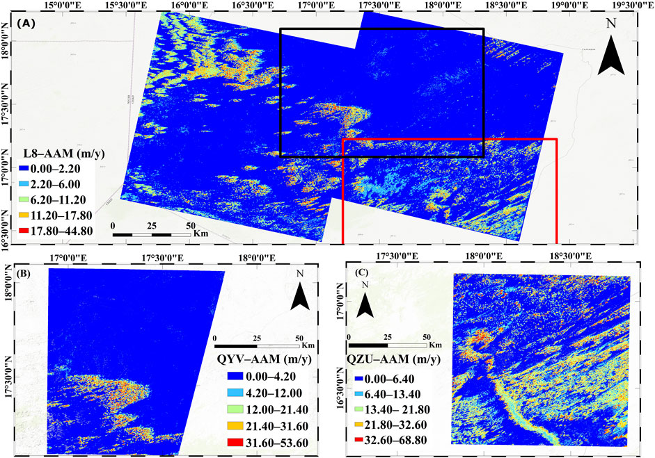
FIGURE 4. Average annual magnitudes of dune migration for Landsat-8 (A) and two Sentinel-2 images: TR33QYV (B) and TR33QZU (C). The black and red polygons in panel (A) denote the coverage of TR33QYV and TR33QZU, respectively. The background is light gray canvas^© using Esri ArcMap 10.3.

FIGURE 5

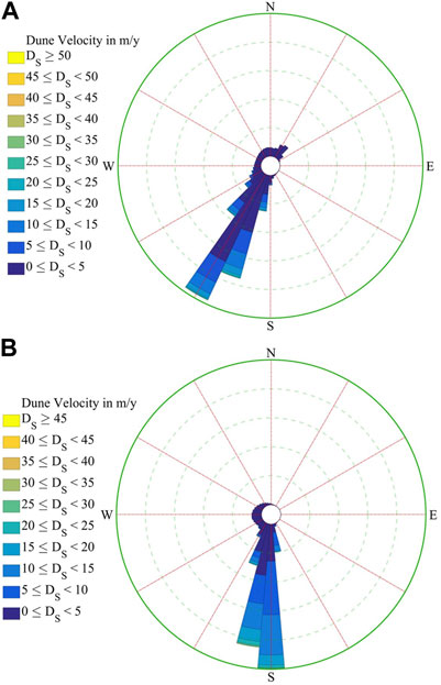
FIGURE 5. Sand roses illustrating the relationship between dune migration rates and migration direction for active dune areas in the Bodélé Depression (A) and the northwestern dune field (B).

4.3 Assessment of Activity Status and Sand Transport

We used the mask generated by the MSC to mask out the stagnant areas. Active aeolian features covered approximately 6,100 km² of the total area of the L-8 frames, and the spatial distribution of the active dune fields is shown in Supplementary Figure S3. Active aeolian features accounted for approximately 1,096 and 2,310 km² within the depression and in the northwestern dune fields, respectively, representing 60% of the active area covered by the L-8 frames. To better capture the abilities of dunes to act as a source of sand supply, move to support other dune fields resulting in variability in dune morphology, or move into stable areas and convert to semi-active/active dune fields, we estimated the area of encroachment (AE) of sand features and dunes, as described by Ding et al. (2020b). We divided the ground covered by the L-8 frames into patches of 100 km², and estimated the AE of each patch. All sand features and dunes associated with each patch were included in the AE calculations. The higher the AE, the greater the ability of the patch to act as a sand supplier. The AEs ranged from 25 to 4,200 m²/y. The spatial distribution of the patch AEs is shown in Supplementary Figure S8. The active dune areas within the BD can encroach approximately ∼530 m²/y, and the dune fields located in the northwest can encroach approximately ∼1,330 m²/y. The average PMDs and CRs of each patch were estimated and displayed in Supplementary Figure S9. The average PMDs of most of the patches were aligned toward the southwest and west, although those of some patches were aligned toward the northeast. The CRs estimated for each patch were higher in the northwestern dune field, while the patches within the BD showed less consistency in their migration directions, revealing large directional variability. This variability within the BD is consistent with Baird et al. (2019), who reported a median directional change of up to 39.26°. This considerable variability in PMDs can be interpreted by the presence of seasonal variations in the prevailing wind direction, changes in the morphology of the sand features, and the complexity of the wind regime. Such directional variability associated for the aeolian features in the BD may interpret the small AE scored in the BD in compared to the Northwest dune field.

4.4 Temporal Evaluation of Dune Migration Patterns

4.4.1 Historical Movement Patterns

We extracted the cumulative displacement time series for 16 sites spatially distributed across the dune fields covered by the L-8 frames (see Figure 1A). These sites were carefully selected for their migration rates to represent the migration patterns across the different dune fields. The median and standard deviation were measured over $3\times 3$ adjacent pixels around each point. Our time series inversion provided continuous monitoring of dune migration patterns for nearly 9 and 6 years, as shown in Figures 6,7, respectively. Some of these points were selected in the overlapping areas between the two sensors, and we compared the time series extracted from the independent sensors with each other and with the fusion between the two sensors (Section 4.6.1). Figure 6 shows the temporal evolution of the points (P01-P08) extracted from the L-8 inversion, whereas points from P09-P16 are displayed in Supplementary Figure S10. The S-2 time series results for nine points located in the ground coverage of the S-2 frames are shown in Figure 7, while the time series results of these points as extracted from the inversion of the fusion between the two sensors are shown in Supplementary Figure S11. The maximum migration rates (∼30 m/y) occurred at points P02, P04, P07, P13, P14, and P16. The minimum migration rate occurred at P06 (∼10 m/y). The other nine points showed moderate migration rates of 15.5–23.5 m/y.

FIGURE 6

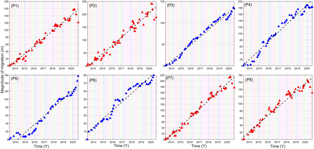
FIGURE 6. Cumulative projected displacements over time extracted from the inversion of the deformation maps belong to two Landsat-8 frames. The dashed colored areas in the background represent the different seasons: red, blue, green, and magenta refer to summer, winter, autumn, and spring, respectively. The black dashed lines denote the best linear fit of the cumulative projected displacement. Red and blue triangles denote the points belonging to the coverage of (183/48) and (184/48), respectively.

FIGURE 7

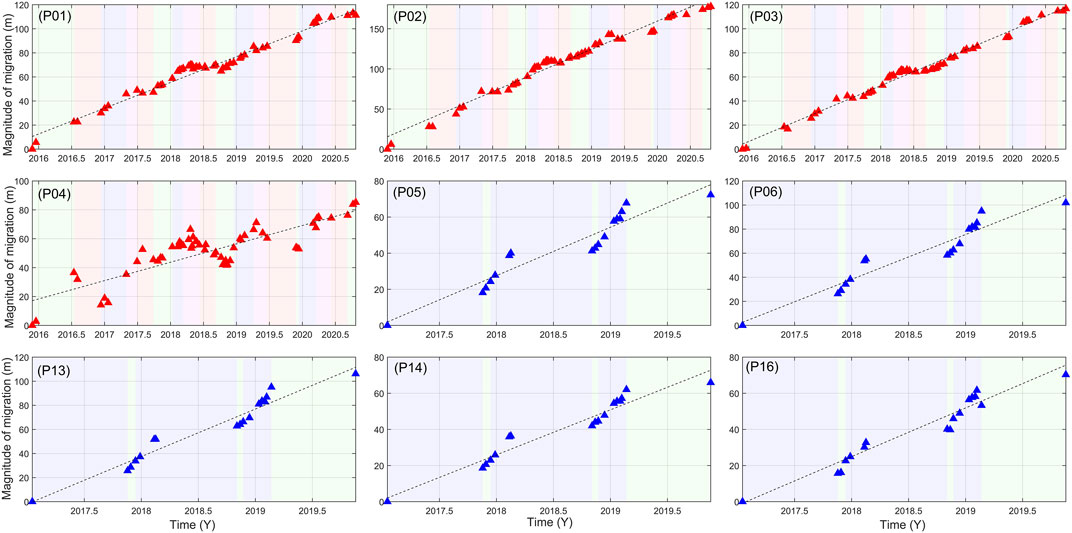
FIGURE 7. Similar to Figure 6, the time series extracted from the inversion of two Sentinel-2 tiles. Red and blue triangles denote the inversion of pairs belonging to T33QYV and T33QZU, respectively.

4.4.2 Seasonality of Movement Patterns and Interpretations

The degree of correlation between the cumulative time series and the best linear fit (black lines, Figures 6, 7) exceeded 97%, showing an almost linear increasing trend. However, seasonal signals in the time series displacements were also observed. To better assess the seasonality in the temporal patterns, we subtracted the value of the linear fit from the CPD (Supplementary Figure S12). The magnitude of the seasonality reached a maximum of ∼30 m/y at points P02 and P03. The presence of these seasonal signals can be attributed to the seasonality of the effective wind regime and dust storms. The seasonality of the dune pattern was supported by observing the direction of migration in each epoch; epochs with a migration direction against the PMD experienced a decrease in net migration. The temporal evolution of the CPDs denoted an inactive status when the migration direction was aligned in the opposite direction to the PMD, leading to a decrease in net migration. Temporally, the dunes experienced lower migration rates during the summer months (i.e., June to August). However, the activity status improved during the winter months, when the dune migration direction was consistent with the PMD. The ECMWF data (see Supplementary Figure S1) showed that the wind was from the northeast in all months except the summer months, when it blew from the southwest. As for the wind speed, the data also showed that the speed reached its minimum values in the summer months. Interestingly, the variability in wind direction was observed in all years from 2013 to 2020, indicating the presence of seasonal fluctuations in the wind regime. As the BD is one of the dustiest places worldwide, dust storms occur frequently, leading to changes in the sand transport system. Previous studies have reported that dust storms are most common in winter because of the northeasterly direction of Bodélé LLJ. These reports are consistent with the observed temporal patterns of dune migration and the activity states extracted from the CPDs. It is assumed that the seasonal signals observed in the time series are not closely coupled with the residuals of seasonal illumination, especially in our study area, which is dry, vegetation-free, and has nearly flat terrain. Consequently, this seasonal variability may be closely related to the activity of the wind regime in the study area. Despite the selection criteria applied to limit the radiometric baselines, which aim to control both seasonal signals and cast shadows, the probability of finding such seasonal signals is still present. Moreover, seasonal signals may be a natural characteristic of dune dynamics owing to the tightly coupled relationship between wind activity and dune migration. It is worth noting that dunes are considered complex monitoring targets compared to glaciers and landslides, as the latter targets are mainly controlled by gravitational forces and melting conditions (Stumpf et al., 2016). Such controlling factors allow filtering out divergent directions from the deformation fields and provide a strong indication of the quality of the matching results and inversion (Stumpf et al., 2016). Consequently, in extracting the time series of dune migration, we paid close attention to the possibility of such seasonal signals being present within the temporal patterns. We attempted to control the presence of divergent seasonal signals through the selection criterion, post-processing, and the projection of the displacement in the PMD, to help capture the true temporal patterns.

4.5 Spatiotemporal Variability of Dune Velocities

4.5.1 Evidence of Spatial Variability of AAMs, MSCs and PMDs

The AAMs, PMDs, and MSCs were analyzed for the ten dune fields, as shown in Figure 8. The AAMs varied spatially between the ten dune fields: 1) The median AAMs value varied from 3.0 to 9.0 m/y, with a maximum value in “Area-10” in the northwest of the study area, consistent with previous results of high encroachment areas in the northwest dune filed. The interquartile values of the active aeolian features varied from 3.85 to 17 m/y. 2) The median PMDs varied from approximately 240–269°, with an interquartile range of 6.2–14.2°, consistent with previous reports of northeasterly winds prevailing in the study area. 3) The median MSC of the active features varied from 0.32 to 0.48. The results of the F-test and Welch’s test are presented in Supplementary Tables S16, S17. The results show that the hypothesis of no significant difference in the means and variance between different dune field pairs can be rejected in most cases, with some exceptions, indicating that the migration rates and corresponding directions varied significantly in the spatial domain. The hypothesis of similar AAM means and variances was accepted for 4 and 3 pairs out of 45 pairs, respectively. The hypothesis of similar PMD means and variances was accepted for 5 pairs out of 45 pairs. Interestingly, the rejection of the hypothesis highlighted spatial variability in the dune migration patterns, which can be attributed to variability in geochemical formation, wind energy, sand transport conditions, dune height and orientation, and wind–topography interactions.

FIGURE 8

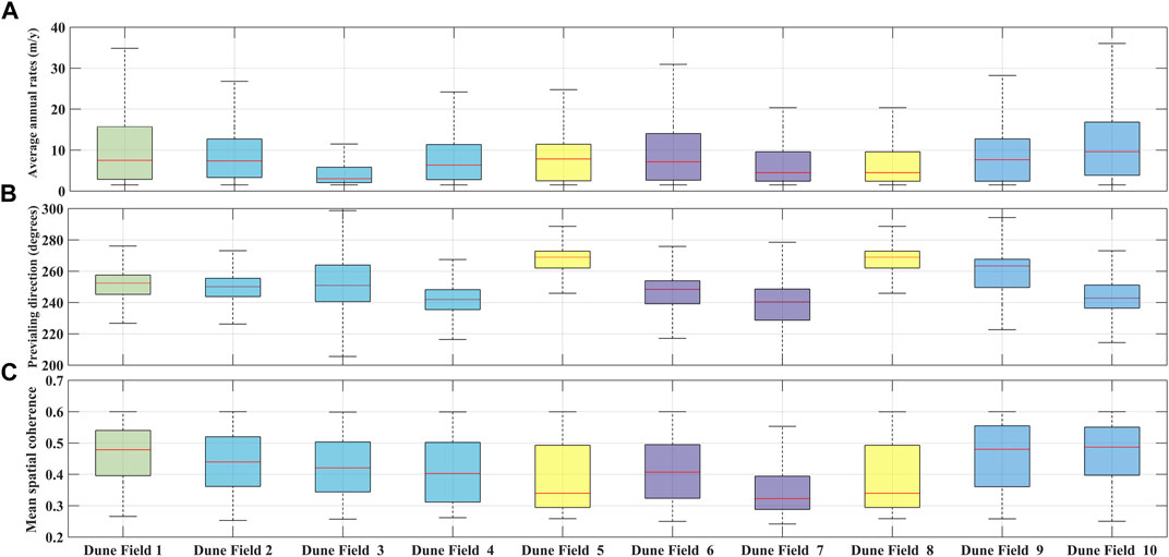
FIGURE 8. Boxplots of the AAM (A), PMD (B), and MSC (C). The box plots were plotted for 4,000 pixels belonging to ten dune fields (see Figure 1). The outliers were discarded from the visualization; however, they were considered in estimating the median, and the interquartile ranges.

4.5.2 Spatiotemporal Variability in Dunes Velocity Between Different Offset Maps

Figure 9 shows boxplots of the estimated geometric means of the active features associated with each dune field extracted from different offset maps, for both migration magnitudes and directions. The median of the geometric mean varied from 11.12 to 17.83 m/y, with an interquartile range of 3.07–12.86 m/y. The geometric means extracted from the AAMs of the same ten dune fields are shown as blue diamonds in Figure 9A. It appears that the fusion of all annual rates tends to underestimate the migration rates; the medians of the geometric means estimated from the AAMs were lower in all cases. This may be attributed to the fact that the fusion of offset maps showing different directions would lead to a reduction in net migration rates. The median of the average directions of the ten dune fields varied between 236.15° and 269.40° with an interquartile range of 3.21°–19.94°. The large interquartile range in “Area 1” may be attributed to the presence of protodunes or sandy patches with variable migration directions. The median CR ranged from 0.117 to 0.928, with an interquartile range of 0.095–0.243. It is worth noting that large CRs indicate the homogeneity of PMDs of active aeolian features associated with each dune field. In particular, the maximum variation in migration direction up to 20° corresponds to a CR of 0.98. The mean values estimated from the PMDs are shown as black diamonds in Figure 9B. The means of the PMDs were nearly identical to the medians of the boxplots, demonstrating the potential of fusion in reliably estimating migration direction.

FIGURE 9

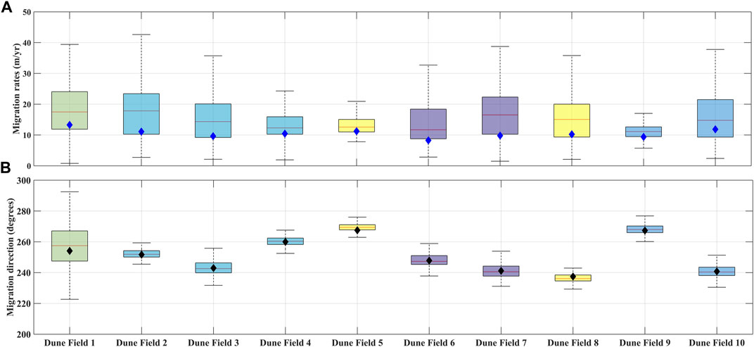
FIGURE 9. Spatiotemporal variability of the dune migration rates (A), and directions (B). Box plots represent the variability of geometric means of dune velocities and the average migration direction of the active aeolian features belonging to each dune field for all the pairs. The blue and black diamonds in (A,B), respectively, represent the geometric means estimated for the active aeolian features belonging to the AAM and PMD solutions.

4.5.3 Spatiotemporal Variability of Dunes Velocities in Different Seasons

Figure 10 shows the variability of the horizontal velocity for ten selected points during the measurement period from 2013 to 2020. The velocity varied during the observation period, with an almost increasing trend during the winter and autumn months. The velocities reached a maximum of ∼220 m/y at P13. Although no clear trend was found to represent the behavior of velocity variation, seasonal variability was observed in the velocity patterns of all the points. The seasonal variability in dune velocity was supported by the wind records extracted from the ECMWF data (Supplementary Figures S13, S14), where the wind speed and direction for the ten selected points were displayed. It was observed that the wind speed showed a fluctuation with lower speeds in the summer months (June to August). Additionally, the wind directions mainly from the northeast with variable directions mainly in summer months. To better capture the seasonal variability in the measured velocity, we estimated the median velocities for the acquisition epochs belonging to each season. Figure 11A shows the variability in the median velocities between different seasons. Interestingly, the median velocities recorded during the summer showed the lowest velocities. We estimated the SSC, which represents the variability of the median velocities between different seasons (Figure 11B). The winter/summer sliding coefficient showed the highest values, ranging from 1.30 to 2.90 with a median of 2.05. In contrast, the median velocities changed slightly in spring and autumn compared to winter, and the median SSCs were 1.14 and 1.36 for winter/spring and winter/autumn, respectively (Figure 11B). The maximum median velocity peaked during the autumn and winter months. The variability in dune velocities at different times of year is expected and can be attributed to seasonal changes in wind strength. The wind records extracted from ECMWF data between 2013 and 2020 (Supplementary Figure S1) showed that the median monthly wind speeds from May to September ranged from 1.20 to 3.40 m/s, with the lowest values in the summer months (June to August). The median wind speed increased up to ∼6.5 m/s in the winter months. In terms of migration direction, the medians of the monthly directions ranged from 233.24° to 250.03° for all months except July and August, when they were 44.95° and 32.74°, respectively. The observed seasonal velocity patterns were consistent with the behavior of the wind regime, and both were consistent with previous reports of the prevailing northeasterly LLJ, especially during winter (Vermeesch and Leprince, 2012).

FIGURE 10

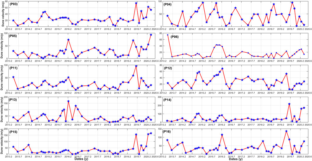
FIGURE 10. Time series of dune velocities as extracted from the inversion of offset maps belong to Landsat-8 frame 183/48. The blue pentagrams represent the acquisition epochs. The red lines denote the continuous dune velocities.

FIGURE 11

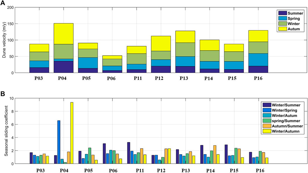
FIGURE 11. Median seasonal velocity at different points belong to Landsat-8 frame 183/48 (A). The seasonal sliding coefficients denote the ratio between the different seasonal velocities (B).

4.5.4 Spatiotemporal Variability of Dune Velocities Between Different Decades (1984–2021)

Figure 12 shows the frequency distributions of the magnitude and direction of the active features within the BD (Figure 1) over three periods (Table 1). The active features within the BD had a strong tendency to migrate toward the southwest and south-southwest; the average migration directions are summarized in Table 1. The differences between the average directions reached a maximum of 3.5°, demonstrating the consistency of the dune migration direction over longer time. Individual examination of the directional differences (Figure 12D) showed variability in the directions between periods 1–2 and between periods 2–3 (Table 1), with median differences of 9.45° and 21.4°, respectively. These individual variations can be attributed to the presence of sand features and protodunes, as well as the formation of new sand features owing to the deflation of sand and dust storms. The large median directional difference between periods 2–3 may also be owing to the high ground resolution of L-8, which could capture more detailed information than Landsat-5. Directional differences of up to 90° may occur owing to change in morphological interactions and the inability of the correlation to capture these morphological changes, especially over longer time intervals. In addition, continuous sand transport and dust storms may affect sand flux in the BD, leading to the birth of new dune generations or the conversion of stable fields to active/semi-active status. The percentage of active areas within the BD ranged from 26 to 30% of the total area, with the lowest value between 2013 and 2021. The geometric mean velocities ranged from 6.61 to 9.66 m/y, with the lowest values recorded for the most recent observation periods. Comparatively, Baird et al. (2019) reported accelerating dune velocities averaging 2.56 ± 12.60 m/y, with some accelerating aeolian elements moving at more than 20 m/y. Here, a comparison between the migration velocities recorded in periods 1 and 2 showed nearly stable conditions with an average acceleration of 0.36 ± 14.20 m/y. In contrast, an average deceleration of 3.2 ± 15.20 m/y was observed when comparing periods 2 and 3. To add new insights to the comparison between migration patterns captured at different observation periods, we compared the average annual wind speed with the geometric mean of the migration rates between similar observation periods. Vermeesch and Leprince (2012) reported that a 1% increase in wind speed results in a ∼3% change in dune velocity and associated dust production. The median annual average wind speeds were 5.24 and 4.84 m/s for periods 2 and 3, respectively, representing a 7.63% decrease in wind speed. The percentage decrease in the migration rate was 28.2%. The ratio between the changes in dune speed and wind speed was approximately 3.50%, which corresponds to the ideal ratio between wind speed and dune speed. The comparison showed strong agreement between the wind speed extracted from the ECMWF and the migration rates estimated from the image matching. However, despite the good agreement between the wind speed and dune velocities, dependence on the matching results rather than the wind speeds could still be considered valuable because 1) the wind speeds from the ECMWF have a coarse resolution (i.e., 0.1 × 0.1 °), 2) the matching measurements can be validated and evaluated, and 3) the matching results provide indications of the migration rates that can be used in vulnerability analysis, stability planning, and modeling.

FIGURE 12

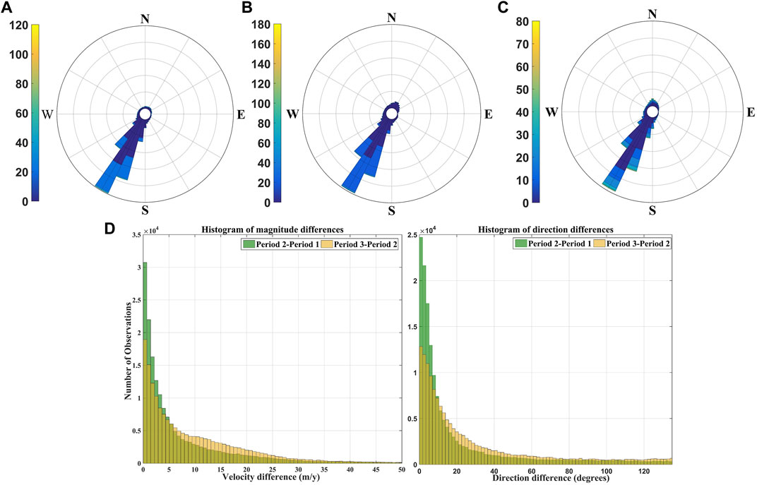
FIGURE 12. Frequency distribution of the active dune and sandy patches in the Bodélé Depression for three observation periods: (A) 1984–1998, (B) 1998–2007, and (C) 2013–2021. Units in (A–C) are in m/y. (D) Histogram of the difference between period 1 and 2 and periods 2 and 3 in terms of magnitude (Right) and direction (Left).

4.6 Validation and Uncertainty Estimation

4.6.1 Cross-Validation

Table 2 summarizes the AAM and PMD values, and the slope of the linear fit for the points covered by L-8 and the points overlapped by L-8 and S-2. There are some inconsistencies between the slope of the linear fit of the CPDs extracted from S-2 and from both L-8 and the fusion; the medians of the absolute difference (MAD) reached ∼4.23 and 6.81 m/y for the differences between S-2/L-8 and S-2/fusion, respectively. The comparison between L-8 and the fusion showed the worst consistency, with a MAD of ∼9.25 m/y. These large differences can be attributed to 1) differences in the observation periods in the S-2 time series and both the L-8 and the fusion time series; 2) the different performance of the inversion networks (i.e., the different condition numbers of the design matrices); and 3) the radical differences in the temporal and spatial resolutions of the sensors and their orthorectification and co-registration accuracy. With respect to AAMs, the comparisons between S-2/L-8 and S-2/fusion showed MADs of ∼7.0 and 6.81 m/y, respectively. The comparison between the AAMs of L-8 and the fusion showed a MAD of 0.7 m/y. Despite the stability of the inversion of one rate owing to large redundancy and good network connectivity, we noticed a larger differences between the AAMs of S-2 and both L-8 and the fusion than between L-8 and the fusion. This can be interpreted by the different observation periods between S-2/L-8 and S-2/fusion. In terms of the PMDs, the directions extracted from S-2 showed strong agreement with both L-8 and the fusion; the MAD were 3.4° and 2.7° for S-2/L-8 and S-2/fusion, respectively. Moreover, the MAD between L-8 and the fusion was 2.5°. From a detailed examination of the temporal patterns extracted from the different inversions, we observed that, for networks with lower temporal sampling (i.e., T33QZU which had only 17-time epochs owing to cloud and haze constraints), the cumulative time series showed two increasing trends with almost stable conditions where no epochs were included (see Figure 7). In comparison, the inversion of TR33QYV captured more details, showing almost linearly increasing trends with low seasonality signals, except for P4 (see Figure 7). However, the fusion between the two sensors (Supplementary Figure S11) provided higher temporal sampling that allowed observation of the temporal evolution up to a weekly time scale. This led to design matrices with higher condition numbers, consequently affecting the stability of the inversion. More seasonality was recorded in the inversion of the merged networks than in the inversions of either L-8 or S-2. The comparisons between the different inversions at different points showed some inconsistencies, especially in the migration magnitudes, but the migration directions showed higher homogeneity regardless of the network configuration and the observation period.

TABLE 2

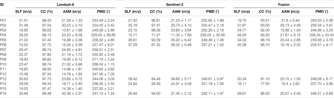
TABLE 2. Slope of linear fit (SLF), correlation coefficient (CC), average annual magnitude (AAM), and prevailing migration direction (PMD) of the test sites from Landsat-8, Sentinel-2, and the fusion between two sensors.

4.6.2 Uncertainty Estimation

We used a stable area of 7.25 km², as shown in Figure 1, to evaluate the uncertainty of the inverted results. We estimated the standard deviation of the measurements as an indicator of uncertainty (Bontemps et al., 2018; Lacroix et al., 2019; Ali et al., 2021). We captured the effect of the inversion in controlling uncertainty by comparing the uncertainties of the individual offset maps before and after inversion (Bontemps et al., 2018). Figure 13 shows the uncertainties of the individual offset maps after inversion and the percentage of improvement in the uncertainties for the L-8 frames. Similar maps for S-2 and the fusion can be found in Supplementary Figure S15. After inversion, the uncertainties varied from 0.27 to 1.90 m and from 0.29 to 1.36 m with averages of 0.70 and 0.62 m for L-8 and S-2, respectively. The percentages of improvement in the uncertainty after inversion were, on average, 35 and 44% for L-8 and S-2, respectively. We also extracted the uncertainties in the inverted results of the CPDs; the uncertainties were, on average, 0.95 m and 0.74 for L-8 and S-2, respectively. It is interesting to note that the uncertainty levels of the inverted results were within the resolution of the matching technique (i.e., about a fifth to a tenth of the ground resolution).

FIGURE 13

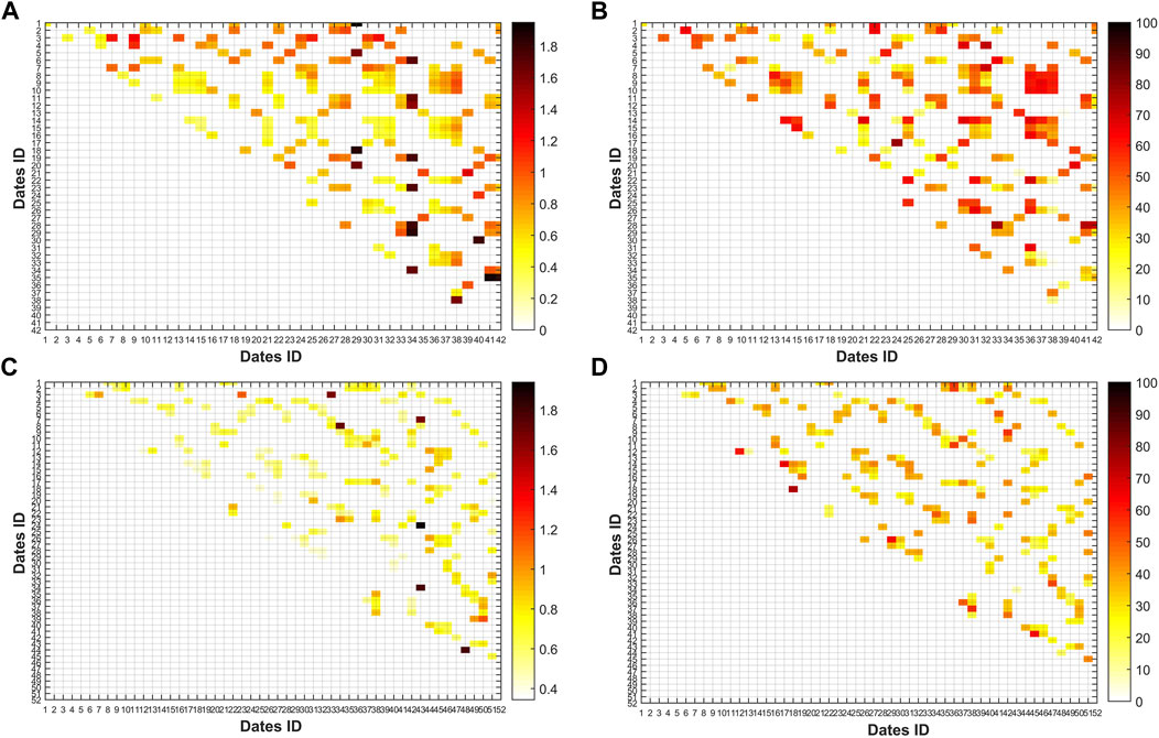
FIGURE 13. Uncertainty of the offset maps after inversion (A) and the percentage of improvement in the uncertainty before and after inversion (B) for the Landsat-8 frame P183/R48. (C) and (D), similar to (A,B) but for the Landsat-8 frame P184/R48. The colored cells represent the pairs with the master on the y-axis and slave on the x-axis. Each pair is defined by the acquisition dates. The acquisition dates of each frame can be found in Supplementary Tables S1, S2. Units in A and C are in (m) while (B, D) are percentages.

4.7 Reflections on Previous Studies

To date, three studies have focused on monitoring dune migration in the BD using optical image matching techniques with different image sources and with different study periods. Vermeesch and Drake (2008) first used a correlation engine with ASTER images at different time intervals and integrated the displacements with dune heights extracted from ASTER stereo images to estimate sand flux. They reported variability in dune velocities, noting that the velocities were 2.5 times higher between December 2006 and January 2007 than between October 2005 and January 2007, and attributed this to the presence of the Bodélé LLJ, which is prevalent during the winter months. A similar trend was observed in our time series, with the winter and summer velocities scoring the highest and the lowest velocities, respectively.

Vermeesch and Leprince (2012) monitored dune acceleration over a 26-year period between 1984 and 2010 using a matching procedure along with seven images from different archives. They used the time series of dune velocities to draw conclusions about the wind conditions in the Sahara Desert, especially in the absence of meteorological observations. They reported that dune velocities of less than 10% over 26 years, equivalent to a ∼0.2% change in wind speed. We believe that the sparse temporal sampling of the extracted time series (i.e., seven images spanning 26 years) missed many details about dune movement and seasonal patterns. In our study, due to the dense temporal sampling, we estimated the median velocity for each season and found that the SSC of the velocities between winter and summer scored ∼2 revealing the activity of the wind in the winter due to the Bodélé LLJ. The effect of acquisition epochs on the temporal patterns was supported in our study, while the inversion of the S2TR33QZU offset maps was limited to 17 epochs due to cloud cover and dust. The inversion showed two increasing linear trends (see Figure 7) with a plateau in between, lacking provide details that can be captured in case of dense acquisition dates. In summary, our study introduced dense spatiotemporal monitoring of dune dynamics and associated drivers inside and outside the BD. It is worth noting that detailed studies on the spatiotemporal patterns of dune dynamics in the BD have been lacking in the literature.

4.8 Contribution of the Inversion of Optical Image Matching for Monitoring the Earth’s Surface

The optical image matching selection and inversion algorithm provides a valuable tool for monitoring surface processes over time, with the advantage of reducing uncertainty and enhancing spatial coverage, especially when using free archives that provide a huge amount of data with dense temporal resolution (Ali et al., 2020; Ding et al., 2020b). As free archives of optical imagery (i.e., L-8 and S-2) offer temporal sampling ranges of 5–16 days, the number of available images is inherently limited by cloud cover, especially in wet seasons in tropical regions (Dille et al., 2021). Limiting the selection of images to those with no/low cloud cover to preserve the matching uncertainty (Lacroix et al., 2018) would affect the number of images and consequently limit the temporal sampling of the time series. Additionally, slow-moving targets require large time separation to help measure real displacement and avoid a large fraction of geolocation errors in the matching results (Fahnestock et al., 2016). However, long temporal baselines affect the temporal sampling of the time series (Dille et al., 2021). Therefore, dependence on the fusion between the time series of two or more sensors with overlapping temporal coverage provides a good alternative to increase the temporal sampling of the time series especially at locations where the images usually contaminated by cloud or haze and enhance understanding of the surface process. In this work, we introduced the fusion of time series from two sensors at overlapping locations to increase the density of the temporal sampling. The comparison between the individual time series from each sensor with the fused time series revealed the potential of the fusion of offset maps with similar ground resolutions in providing dense temporal sampling at up to a weekly time scale. The fusion procedure avoids the high computational costs and data burdens associated with the inversion of a full network. However, fusion provides higher inversion ratios, and the configuration of the network and condition number of the matrix should be considered to preserve the quality of the inverted results. The density of the temporal sampling of the time series can, therefore, be improved by matching images from different sensors, considering the effect of the radiometric variation of both images (Necsoiu et al., 2009). Although the matching of different sensors would provide a simple framework for inversion, differences in the radiometric properties and Sun angles between the two images could affect the quality of the offset maps. Matching networks created via matching images from different sensors can be applied to guarantee good connectivity of the design network and dense temporal sampling, revealing the complex patterns of surface deformations.

5 Conclusion

In this work, we extended the application of the optical image matching selection and inversion algorithm using L-8 and S-2 data to gain new insights into the spatiotemporal patterns of dune migration in the BD during 2013–2021. Images from the L-8 and S-2 archives with low cloud cover were selected to control uncertainty and improve spatial coverage. The selected images were used to generate networks of matched pairs by setting radiometric and temporal baselines. Using the MSC, stagnant and moving targets were automatically differentiated. The inversion was performed using a pixel-by-pixel strategy and flexible design matrices that covered a large area (up to 98% of the total area of the two L-8 frames). The AAMs and their corresponding PMDs exhibited large spatial variability that can be attributed to various factors such as soil moisture, soil particles, sand transport, wind energy, and wind–topography interactions. The PMDs showed a tendency of migration toward the southwest, which is consistent with the prevailing northeasterly direction of the Bodélé LLJ. The temporal patterns of dune migration showed significant seasonal variation, which can be attributed to the seasonality of the effective wind regimes and dust storms. The average monthly wind speeds and directions extracted from the ECMWF showed that northeasterly winds were predominant in all months except the summer months. In addition, the wind speed was lowest during the summer months and highest during winter. Comparison between the inversions of the different networks showed some discrepancies owing to the different performances of the inversions, based on the different networks. Inversion reduced the uncertainty by, on average, 35 and 44% for L-8 and S-2, respectively. In addition, fusion between the two sensors allowed the temporal sampling to be condensed to reveal complex short-term patterns of surface deformation. The fusion of two or more sensors would be a promising alternative for monitoring temporal evolution with dense temporal coverage, especially in regions with heavy cloud cover in tropical areas.

Data Availability Statement

The original contributions presented in the study are included in the article/Supplementary Material, further inquiries can be directed to the corresponding author.

Author Contributions

EA: Writing-original draft, conceptualization, methodology, investigation, validation, and visualization. WX: Conceptualization, investigation, writing—review and editing, and supervision. LX: Writing—review and editing, Visualization. XD: Funding acquisition, Writing—review and editing, supervision. All authors were involved in the final preparation of the draft and have read and approved the manuscript.

Funding

This research was jointly supported by the Research Grants Council (RGC) of the Hong Kong Special Administrative Region (PolyU 152232/17E, PolyU 152164/18E, and PolyU 152233/19E), the Research Institute for Sustainable Urban Development (RISUD), the Hong Kong Polytechnic University, and the Innovative Technology Fund (ITP/019/20LP).

Conflict of Interest

The authors declare that the research was conducted in the absence of any commercial or financial relationships that could be construed as a potential conflict of interest.

Publisher’s Note

All claims expressed in this article are solely those of the authors and do not necessarily represent those of their affiliated organizations, or those of the publisher, the editors and the reviewers. Any product that may be evaluated in this article, or claim that may be made by its manufacturer, is not guaranteed or endorsed by the publisher.

Acknowledgments

We are extremely grateful to the ESA for providing the Copernicus Sentinel-2 data through the Sentinel Science Hub and the Sentinel-2 Expert Users Data Hub, to the USGS for providing the Landsat data through Earth Explorer http://earthexplorer.usgs.gov/, to the European Center for Medium-Range Weather Forecasts (ECMWF) for providing the wind records, to Alaska Satellite Facility https://www.ecmwf.int/ for providing the Sentinel-1A data, and to the Caltech Group for providing COSI-Corr. We used ArcMap 10.3 software for map generation and spatial analysis. We also used MATLAB 2016a for coding and scripting.

Supplementary Material

The Supplementary Material for this article can be found online at: https://www.frontiersin.org/articles/10.3389/fenvs.2021.808802/full#supplementary-material

References

Agram, P. S., Gurrola, E. M., Agram, P., Cohen, J., Lavalle, M., and Riel, B. V. (2016). “The InSAR Scientific Computing Environment 3.0: a Flexible Framework for InSAR Operational and User-Led Science Processing,” in AGU Fall Meeting Abstracts (United States: AGU), 4901–4904.

Google Scholar

Ahmady-Birgani, H., McQueen, K. G., Moeinaddini, M., and Naseri, H. (2017). Sand Dune Encroachment and Desertification Processes of the Rigboland Sand Sea, Central Iran. Sci. Rep. 7, 1523. doi:10.1038/s41598-017-01796-z

PubMed Abstract | CrossRef Full Text | Google Scholar

Ali, E., and Xu, W. (2019). “An Optical Image Time Series Inversion Method and Application to Long Term Sand Dune Movements in the Sinai Peninsula,” in European Geosciences Union (Vienna, Austria: EGU).

Google Scholar

Ali, E., Xu, W., and Ding, X. (2020). Improved Optical Image Matching Time Series Inversion Approach for Monitoring Dune Migration in North Sinai Sand Sea: Algorithm Procedure, Application, and Validation. ISPRS J. Photogrammetry Remote Sensing 164, 106–124. doi:10.1016/j.isprsjprs.2020.04.004

CrossRef Full Text | Google Scholar

Ali, E., Xu, W., and Ding, X. (2021). Spatiotemporal Variability of Dune Velocities and Corresponding Uncertainties, Detected from Optical Image Matching in the North Sinai Sand Sea, Egypt. Remote Sensing 13, 3694. doi:10.3390/rs13183694

CrossRef Full Text | Google Scholar

Altena, B., Scambos, T., Fahnestock, M., and Kääb, A. (2019). Extracting Recent Short-Term Glacier Velocity Evolution Over Southern Alaska and the Yukon From a Large Collection of Landsat Data. Cryosph 13, 795–814. doi:10.5194/tc-13-795-2019

CrossRef Full Text | Google Scholar

Avouac, J.-P., Ayoub, F., Wei, S., Ampuero, J.-P., Meng, L., Leprince, S., et al. (2014). The 2013, Mw 7.7 Balochistan Earthquake, Energetic Strike-Slip Reactivation of a Thrust Fault. Earth Planet. Sci. Lett. 391, 128–134. doi:10.1016/j.epsl.2014.01.036

CrossRef Full Text | Google Scholar

Ayoub, F., Leprince, S., and Avouac, J.-P. (2009). Co-registration and Correlation of Aerial Photographs for Ground Deformation Measurements. ISPRS J. Photogrammetry Remote Sensing 64, 551–560. doi:10.1016/j.isprsjprs.2009.03.005

CrossRef Full Text | Google Scholar

Baird, T., Bristow, C., and Vermeesch, P. (2019). Measuring Sand Dune Migration Rates with COSI-Corr and Landsat: Opportunities and Challenges. Remote Sensing 11, 2423. doi:10.3390/rs11202423

CrossRef Full Text | Google Scholar

Beaud, F., Aati, S., Delaney, I., Adhikari, S., and Avouac, J.-P. (2021). Generalized Sliding Law Applied to the Surge Dynamics of Shisper Glacier and Constrained by Timeseries Correlation of Optical Satellite Images. Cryosph. Discuss. 4, 1–35. doi:10.5194/tc-2021-96

CrossRef Full Text | Google Scholar

Berardino, P., Fornaro, G., Lanari, R., and Sansosti, E. (2002). A New Algorithm for Surface Deformation Monitoring Based on Small Baseline Differential SAR Interferograms. IEEE Trans. Geosci. Remote Sensing 40, 2375–2383. doi:10.1109/TGRS.2002.803792

CrossRef Full Text | Google Scholar

Bontemps, N., Lacroix, P., and Doin, M.-P. (2018). Inversion of Deformation fields Time-Series from Optical Images, and Application to the Long Term Kinematics of Slow-Moving Landslides in Peru. Remote Sensing Environ. 210, 144–158. doi:10.1016/j.rse.2018.02.023

CrossRef Full Text | Google Scholar

Bristow, C. S., Drake, N., and Armitage, S. (2009). Deflation in the Dustiest Place on Earth: The Bodélé Depression, Chad. Geomorphology 105, 50–58. doi:10.1016/j.geomorph.2007.12.014

CrossRef Full Text | Google Scholar

Bui, L. K., Featherstone, W. E., and Filmer, M. S. (2020). Disruptive Influences of Residual Noise, Network Configuration and Data Gaps on InSAR-Derived Land Motion Rates Using the SBAS Technique. Remote Sens. Environ. 247, 111941. doi:10.1016/j.rse.2020.111941

CrossRef Full Text | Google Scholar

Chappell, A., and Bristow, C. (2005). Dustiest Place on Earth. Nature 434, 1.

Google Scholar

Chen, K., Avouac, J.-P., Aati, S., Milliner, C., Zheng, F., and Shi, C. (2020). Cascading and Pulse-like Ruptures during the 2019 Ridgecrest Earthquakes in the Eastern California Shear Zone. Nat. Commun. 11, 3–10. doi:10.1038/s41467-019-13750-w

PubMed Abstract | CrossRef Full Text | Google Scholar

Das, S., and Sharma, M. C. (2021). Glacier Surface Velocities in the Jankar Chhu Watershed, Western Himalaya, India: Study Using Landsat Time Series Data (1992-2020). Remote Sensing Appl. Soc. Environ. 24, 100615. doi:10.1016/j.rsase.2021.100615

CrossRef Full Text | Google Scholar

Dee, D. P., Uppala, S. M., Simmons, A. J., Berrisford, P., Poli, P., Kobayashi, S., et al. (2011). The ERA-Interim Reanalysis: Configuration and Performance of the Data Assimilation System. Q.J.R. Meteorol. Soc. 137, 553–597. doi:10.1002/qj.828

CrossRef Full Text | Google Scholar

Dille, A., Kervyn, F., Handwerger, A. L., d'Oreye, N., Derauw, D., Mugaruka Bibentyo, T., et al. (2021). When Image Correlation Is Needed: Unravelling the Complex Dynamics of a Slow-Moving Landslide in the Tropics with Dense Radar and Optical Time Series. Remote Sensing Environ. 258, 112402. doi:10.1016/j.rse.2021.112402

CrossRef Full Text | Google Scholar

Ding, C., Feng, G., Liao, M., Tao, P., Zhang, L., and Xu, Q. (2021). Displacement History and Potential Triggering Factors of Baige Landslides, China Revealed by Optical Imagery Time Series. Remote Sensing Environ. 254, 112253. doi:10.1016/j.rse.2020.112253

CrossRef Full Text | Google Scholar

Ding, C., Feng, G., Liao, M., and Zhang, L. (2020a). Change Detection, Risk Assessment and Mass Balance of mobile Dune fields Near Dunhuang Oasis with Optical Imagery and Global Terrain Datasets. Int. J. Digital Earth 13, 1604–1623. doi:10.1080/17538947.2020.1767222

CrossRef Full Text | Google Scholar

Ding, C., Zhang, L., Liao, M., Feng, G., Dong, J., Ao, M., et al. (2020b). Quantifying the Spatio-Temporal Patterns of Dune Migration Near Minqin Oasis in Northwestern China with Time Series of Landsat-8 and Sentinel-2 Observations. Remote Sensing Environ. 236, 111498. doi:10.1016/j.rse.2019.111498

CrossRef Full Text | Google Scholar

El-magd, I. A., Hassan, O., and Arafat, S. (2013). Quantification of Sand Dune Movements in the South Western Part of Egypt, Using Remotely Sensed Data and GIS. Jgis 05, 498–508. doi:10.4236/jgis.2013.55047

CrossRef Full Text | Google Scholar

Fahnestock, M., Scambos, T., Moon, T., Gardner, A., Haran, T., and Klinger, M. (2016). Rapid Large-Area Mapping of Ice Flow Using Landsat 8. Remote Sensing Environ. 185, 84–94. doi:10.1016/j.rse.2015.11.023

CrossRef Full Text | Google Scholar

Farr, T. G., Rosen, P. A., Caro, E., Crippen, R., Duren, R., Hensley, S., et al. (2007). The Shuttle Radar Topography Mission. Rev. Geophys. 45, RG2004. doi:10.1029/2005RG000183

CrossRef Full Text | Google Scholar

Fattahi, H., Agram, P., and Simons, M. (2017). A Network-Based Enhanced Spectral Diversity Approach for TOPS Time-Series Analysis. IEEE Trans. Geosci. Remote Sensing 55, 777–786. doi:10.1109/TGRS.2016.2614925

CrossRef Full Text | Google Scholar

Friedl, P., Seehaus, T., and Braun, M. (2021). Global Time Series and Temporal Mosaics of Glacier Surface Velocities, Derived From Sentinel-1 Data. Earth Syst. Sci. Data Discuss., 1–33. doi:10.5194/essd-2021-106

CrossRef Full Text | Google Scholar

Gaber, A., Abdelkareem, M., Abdelsadek, I., Koch, M., and El-Baz, F. (2018). Using InSAR Coherence for Investigating the Interplay of Fluvial and Aeolian Features in Arid Lands: Implications for Groundwater Potential in Egypt. Remote Sens. 10, 1–18. doi:10.3390/rs10060832

CrossRef Full Text | Google Scholar

Ghadiry, M., Shalaby, A., and Koch, B. (2012). A New GIS-Based Model for Automated Extraction of Sand Dune Encroachment Case Study: Dakhla Oases, Western Desert of Egypt. Egypt. J. Remote Sensing Space Sci. 15, 53–65. doi:10.1016/j.ejrs.2012.04.001

CrossRef Full Text | Google Scholar

Goudie, A. S., and Middleton, N. J. (2001). Saharan Dust Storms: Nature and Consequences. Earth-Science Rev. 56, 179–204. doi:10.1016/S0012-8252(01)00067-8

CrossRef Full Text | Google Scholar

Hamdan, M. A., Refaat, A. A., and Abdel Wahed, M. (2016). Morphologic Characteristics and Migration Rate Assessment of Barchan Dunes in the Southeastern Western Desert of Egypt. Geomorphology 257, 57–74. doi:10.1016/j.geomorph.2015.12.026

CrossRef Full Text | Google Scholar

Hereher, M. E. (2010). Sand Movement Patterns in the Western Desert of Egypt: an Environmental Concern. Environ. Earth Sci. 59, 1119–1127. doi:10.1007/s12665-009-0102-9

CrossRef Full Text | Google Scholar

Hermas, E., Alharbi, O., Alqurashi, A., Niang, A. J., Al-Ghamdi, K., Al-Mutiry, M., et al. (2019). Characterisation of Sand Accumulations in Wadi Fatmah and Wadi Ash Shumaysi, KSA, Using Multi-Source Remote Sensing Imagery. Remote Sensing 11, 2824. doi:10.3390/rs11232824

CrossRef Full Text | Google Scholar

Hermas, E., Leprince, S., and El-Magd, I. A. (2012). Retrieving Sand Dune Movements Using Sub-pixel Correlation of Multi-Temporal Optical Remote Sensing Imagery, Northwest Sinai Peninsula, Egypt. Remote Sensing Environ. 121, 51–60. doi:10.1016/j.rse.2012.01.002

CrossRef Full Text | Google Scholar

Hudson-Edwards, K. A., Bristow, C. S., Cibin, G., Mason, G., and Peacock, C. L. (2014). Solid-Phase Phosphorus Speciation in Saharan Bodélé Depression Dusts and Source Sediments. Chem. Geol. 384, 16–26. doi:10.1016/j.chemgeo.2014.06.014

CrossRef Full Text | Google Scholar

Hugenholtz, C. H., Levin, N., Barchyn, T. E., and Baddock, M. C. (2012). Remote Sensing and Spatial Analysis of Aeolian Sand Dunes: A Review and Outlook. Earth-Science Rev. 111, 319–334. doi:10.1016/j.earscirev.2011.11.006

CrossRef Full Text | Google Scholar

Jawak, S. D., Kumar, S., Luis, A. J., Bartanwala, M., Tummala, S., and Pandey, A. C. (2018). Evaluation of Geospatial Tools for Generating Accurate Glacier Velocity Maps from Optical Remote Sensing Data. Proceedings 2, 341. doi:10.3390/ecrs-2-05154

CrossRef Full Text | Google Scholar

Kääb, A., Winsvold, S., Altena, B., Nuth, C., Nagler, T., and Wuite, J. (2016). Glacier Remote Sensing Using Sentinel-2. Part I: Radiometric and Geometric Performance, and Application to Ice Velocity. Remote Sensing 8, 598. doi:10.3390/rs8070598

CrossRef Full Text | Google Scholar

Koren, I., Kaufman, Y. J., Washington, R., Todd, M. C., Rudich, Y., Martins, J. V., et al. (2006). The Bodélé Depression: a Single Spot in the Sahara that Provides Most of the mineral Dust to the Amazon forest. Environ. Res. Lett. 1, 014005. doi:10.1088/1748-9326/1/1/014005

CrossRef Full Text | Google Scholar

Lacroix, P., Araujo, G., Hollingsworth, J., and Taipe, E. (2019). Self‐Entrainment Motion of a Slow‐Moving Landslide Inferred from Landsat‐8 Time Series. J. Geophys. Res. Earth Surf. 124, 1201–1216. doi:10.1029/2018JF004920

CrossRef Full Text | Google Scholar

Lacroix, P., Bièvre, G., Pathier, E., Kniess, U., and Jongmans, D. (2018). Use of Sentinel-2 Images for the Detection of Precursory Motions before Landslide Failures. Remote Sensing Environ. 215, 507–516. doi:10.1016/j.rse.2018.03.042

CrossRef Full Text | Google Scholar

Leprince, S., Barbot, S., Ayoub, F., and Avouac, J.-P. (2007). Automatic and Precise Orthorectification, Coregistration, and Subpixel Correlation of Satellite Images, Application to Ground Deformation Measurements. IEEE Trans. Geosci. Remote Sensing 45, 1529–1558. doi:10.1109/TGRS.2006.888937

CrossRef Full Text | Google Scholar

Manzoni, M., Molinari, M. E., and Monti-Guarnieri, A. (2021). Multitemporal inSAR Coherence Analysis and Methods for Sand Mitigation. Remote Sensing 13, 1362. doi:10.3390/rs13071362

CrossRef Full Text | Google Scholar

Middleton, N. J., and Sternberg, T. (2013). Climate Hazards in Drylands: A Review. Earth-Science Rev. 126, 48–57. doi:10.1016/j.earscirev.2013.07.008

CrossRef Full Text | Google Scholar

Mouginot, J., Rignot, E., Scheuchl, B., and Millan, R. (2017). Comprehensive Annual Ice Sheet Velocity Mapping Using Landsat-8, Sentinel-1, and RADARSAT-2 Data. Remote Sensing 9, 364. doi:10.3390/rs9040364

CrossRef Full Text | Google Scholar

Necsoiu, M., Leprince, S., Hooper, D. M., Dinwiddie, C. L., McGinnis, R. N., and Walter, G. R. (2009). Monitoring Migration Rates of an Active Subarctic Dune Field Using Optical Imagery. Remote Sensing Environ. 113, 2441–2447. doi:10.1016/j.rse.2009.07.004

CrossRef Full Text | Google Scholar

Reinisch, E. C., Cardiff, M., and Feigl, K. L. (2017). Graph Theory for Analyzing Pair-wise Data: Application to Geophysical Model Parameters Estimated from Interferometric Synthetic Aperture Radar Data at Okmok Volcano, Alaska. J. Geod. 91, 9–24. doi:10.1007/s00190-016-0934-5

CrossRef Full Text | Google Scholar

Rouyet, L., Lauknes, T. R., Christiansen, H. H., Strand, S. M., and Larsen, Y. (2019). Seasonal Dynamics of a Permafrost Landscape, Adventdalen, Svalbard, Investigated by InSAR. Remote Sensing Environ. 231, 111236. doi:10.1016/j.rse.2019.111236

CrossRef Full Text | Google Scholar

Roy, D. P., Wulder, M. A., Loveland, T. R., Woodcook, C. E., Anderson, M. C., Helder, D., et al. (2014). Landsat-8: Science and Product Vision for Terrestrial Global Change Research. Remote Sensing Environ. 145, 154–172. doi:10.1016/j.rse.2014.02.001

CrossRef Full Text | Google Scholar

Rozenstein, O., Siegal, Z., Blumberg, D. G., and Adamowski, J. (2016). Investigating the Backscatter Contrast Anomaly in Synthetic Aperture Radar (SAR) Imagery of the Dunes along the Israel-Egypt Border. Int. J. Appl. Earth Observation Geoinformation 46, 13–21. doi:10.1016/j.jag.2015.11.008

CrossRef Full Text | Google Scholar

Sam, L., Gahlot, N., and Prusty, B. G. (2015). Estimation of Dune Celerity and Sand Flux in Part of West Rajasthan, Gadra Area of the Thar Desert Using Temporal Remote Sensing Data. Arab. J. Geosci. 8, 295–306. doi:10.1007/s12517-013-1219-4

CrossRef Full Text | Google Scholar

Samsonov, S., Tiampo, K., and Cassotto, R. (2020). Measuring the State and Temporal Evolution of Glaciers Using SAR-Derived 3D Time Series of Glacier Surface Flow. Cryosph. Discuss. 34, 1–21. doi:10.5194/tc-2020-257

CrossRef Full Text | Google Scholar

Scheidt, S. P., and Lancaster, N. (2013). The Application of COSI-Corr to Determine Dune System Dynamics in the Southern Namib Desert Using ASTER Data. Earth Surf. Process. Landforms 38, 1004–1019. doi:10.1002/esp.3383

CrossRef Full Text | Google Scholar

Scherler, D., Leprince, S., and Strecker, M. (2008). Glacier-surface Velocities in alpine Terrain from Optical Satellite Imagery-Accuracy Improvement and Quality Assessment. Remote Sensing Environ. 112, 3806–3819. doi:10.1016/j.rse.2008.05.018

CrossRef Full Text | Google Scholar

Shukla, A., and Garg, P. K. (2020). Spatio-temporal Trends in the Surface Ice Velocities of the central Himalayan Glaciers, India. Glob. Planet. Change 190, 103187. doi:10.1016/j.gloplacha.2020.103187

CrossRef Full Text | Google Scholar

Stravalaci, M., Davi, F., Parente, R., Gobbi, M., Bottazzi, B., Mantovani, A., et al. (2020). Control of Complement Activation by the Long Pentraxin PTX3: Implications in Age-Related Macular Degeneration. Front. Pharmacol. 11, 591908. doi:10.3389/fphar.2020.591908

PubMed Abstract | CrossRef Full Text | Google Scholar

Stumpf, A., Malet, J.-P., Allemand, P., and Ulrich, P. (2014). Surface Reconstruction and Landslide Displacement Measurements with Pléiades Satellite Images. ISPRS J. Photogrammetry Remote Sensing 95, 1–12. doi:10.1016/j.isprsjprs.2014.05.008

CrossRef Full Text | Google Scholar

Stumpf, A., Malet, J.-P., Puissant, A., and Travelletti, J. (2016). “Monitoring of Earth Surface Motion and Geomorphologic Processes by Optical Image Correlation,” in Land Surface Remote Sensing (Elsevier), 147–190. doi:10.1016/B978-1-78548-105-5.50005-0

CrossRef Full Text | Google Scholar

Touzi, R., Lopes, A., Bruniquel, J., and Vachon, P. W. (1999). Coherence Estimation for SAR Imagery. IEEE Trans. Geosci. Remote Sensing 37, 135–149. doi:10.1109/36.739146

CrossRef Full Text | Google Scholar

Ullmann, T., Sauerbrey, J., Hoffmeister, D., May, S. M., Baumhauer, R., and Bubenzer, O. (2019). Assessing Spatiotemporal Variations of Sentinel-1 InSAR Coherence at Different Time Scales Over the Atacama Desert (Chile) Between 2015 and 2018. Remote Sens. 11, 2960. doi:10.3390/rs11242960

CrossRef Full Text | Google Scholar

Usai, S. (2003). A Least Squares Database Approach for SAR Interferometric Data. IEEE Trans. Geosci. Remote Sensing 41, 753–760. doi:10.1109/TGRS.2003.810675

CrossRef Full Text | Google Scholar

Vermeesch, P., and Drake, N. (2008). Remotely Sensed Dune Celerity and Sand Flux Measurements of the World's Fastest Barchans (Bodélé, Chad). Geophys. Res. Lett. 35, 1–6. doi:10.1029/2008GL035921

CrossRef Full Text | Google Scholar

Vermeesch, P., and Leprince, S. (2012). A 45-year Time Series of Dune Mobility Indicating Constant Windiness over the central Sahara. Geophys. Res. Lett. 39, a–n. doi:10.1029/2012GL052592

CrossRef Full Text | Google Scholar

Warren, A., Chappell, A., Todd, M. C., Bristow, C., Drake, N., Engelstaedter, S., et al. (2007). Dust-raising in the Dustiest Place on Earth. Geomorphology 92, 25–37. doi:10.1016/j.geomorph.2007.02.007

CrossRef Full Text | Google Scholar

Washington, R., Todd, M. C., Lizcano, G., Tegen, I., Flamant, C., Koren, I., et al. (2006). Links between Topography, Wind, Deflation, Lakes and Dust: The Case of the Bodélé Depression, Chad. Geophys. Res. Lett. 33, 1–4. doi:10.1029/2006GL025827

CrossRef Full Text | Google Scholar

Wegmüller, U., Strozzi, T., Farr, T., and Werner, C. L. (2000). Arid Land Surface Characterization With Repeat-Pass SAR Interferometry. IEEE Trans. Geosci. Remote Sens. 38, 776–781. doi:10.1109/36.842006

CrossRef Full Text | Google Scholar

Yang, W., Fang, J., and Liu-Zeng, J. (2021). Landslide-lake Outburst Floods Accelerate Downstream Slope Slippage. Earth Surf. Dyn. Discuss. 2021, 1–19.

Google Scholar