Tracking chlorinated contaminants in the subsurface using analytical, numerical and geophysical methods

1 Introduction

Generally, the distribution of contamination sources and the emission of contamination concentration need to be found out before the contamination is treated and remediated effectively. However, groundwater contamination has the characteristics of concealment, hysteresis and irreversibility, which makes it impossible to detect contamination sources in time after contamination occurs with continuous spreading. Therefore, tracing, locating and removing contamination sources are important steps for the site risk management. The key problem is to determine the contamination sources accurately and timely. Therefore, it is important to identify the location of groundwater contamination sources, contaminant emission concentration and development history, so as to take effective measures to cut off the contamination sources and avoid the contamination of groundwater in a wider range, furthermore, it has an important impact on the efficiency and cost of subsequent remediation (Mangold and Tsang, 1991; Bashi-Azghadi et al., 2010; Lapworth et al., 2012; Mahsa and Bithin, 2013).

Traceability of groundwater contamination is to trace the history of contaminant discharge and determine the location of contamination sources through limited observation data (Mahar and Datta, 1997; Alexander et al., 2006; Zoi and George, 2009). At present, the main methods of groundwater contamination traceability are mathematical analysis method (Gongsheng et al., 2006; Yu et al., 2012; Long et al., 2014; Gurarslan and Karahan, 2015), simulation optimization method (Ellen and Pierre, 2007; Mirghani et al., 2009; Manish and Bithin, 2013; Xiao et al., 2016; Li et al., 2017; Chakraborty and Prakash, 2020), hydrochemical traceability analysis (; Rashid et al., 2019), isotope traceability analysis (Palau et al., 2014; Sturchio et al., 2014; Nigro et al., 2017; Wang and Zhang, 2019; Zimmermann et al., 2020) and geostatistics method (Mark and Peter, 1997; Juliana and Amvrossios, 2001; Ilaria and Maria, 2003; Anna and Peter, 2004; Ilaria et al., 2012; Liu et al., 2021). The contamination factors mainly occur convection, dispersion and microbial reactions after the contaminants are released into subsurface (Jordi and Yoram, 1996). While the traceability of contamination sources can be solved as a reverse problem by combining the information of groundwater contamination plume with the law of contaminant migration (Gurarslan and Karahan, 2015), in addition, the most commonly used methods are numerical method and analytical method based on the mathematical model of contaminant migration in saturated-unsaturated porous media.

The numerical simulation of groundwater contamination is mainly to study the temporal and spatial variation of the concentration of various solutes in porous media, and predict the distribution of contaminants qualitatively or quantitatively (Song et al., 2020; Banaei et al., 2021). For example, the convection-dispersion model has a wide range of applications, which can be used for isotropic or anisotropic, homogeneous or heterogeneous porous media (Wu et al., 1997; Zhu and Liu, 2001). It can reflect the movement process of solute in groundwater comprehensively under the initial conditions and boundary conditions, and it has become a very important method to solve the problem of groundwater contamination with the continuous and rapid development of science technology. In addition, it is widely used in the field of hydrogeology with its convenient, efficient and flexible characteristics (Xue, 2010). However, the establishment of numerical model requires much higher accuracy of hydrogeological data than the analytical method, and more detailed data are needed for the model identification and verification. For example, the number of monitoring wells in the field investigation stage is relatively small in the internal area of chemical plants which facilities have been completed, thus, it is often not desirable to drill new monitoring wells, therefore, the analytical method is still widely used under above conditions.

In this paper, taking the actual site as an example, mathematical models are established through the generalization of practical problems, and the analytical method is applied to trace the emission process of contamination sources, and then the location and emission process of contamination sources are inverted. In addition, the influence of observation point layout, hydrodynamic dispersion coefficient and actual velocity on the traceability results is discussed by numerical simulation.

Then, the numerical method and analytical method are used to predict the spatial range and diachronic process of chloride in contamination sources, and the results are verified by the geophysical prospecting and drilling sampling analysis, moreover, the diffusion range and diachronic process of chloride are determined based on the analysis of the difference between the predicted results and the measured results. Finally, the suitability of the analytical method in this region is discussed, indicating that the method proposed in this paper is effective, and also it provides a feasible tool for solving the problem of contamination source research in-scale sites, furthermore, it provides a feasible technically and reasonable economical method for contamination source traceability and remediation design under such hydrogeological conditions.

2 Materials and methods

2.1 Study area overview

The research site is located in the central and eastern part of Hefei, Anhui Province, China (Figure 1). In order to investigate the stratigraphic characteristics of the region, high-density resistivity method and ground penetrating radar method were used in this detection, and the hydraulic crawler multifunctional engineering investigation rig was used for drilling. The soil core samples were collected and the corresponding soil samples were obtained. According to the above survey results, the target area is mainly divided into two layers, 1) the principal component of miscellaneous fill layer is clay, surface soil plant roots are more developed and the layer thickness is about 2 m. 2) the thickness of clay layer exceeds 10 m under natural conditions.

FIGURE 1

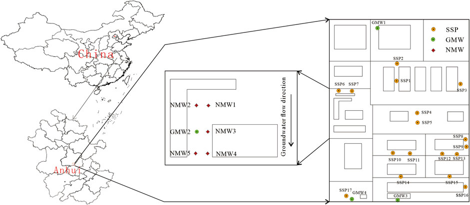
FIGURE 1. Locations of the soil sampling points and groundwater monitoring wells in the study.

2.2 Analytical method

According to the actual survey and test data, the migration trend of chloride in GMW2 monitoring point is mainly vertical migration. Therefore, the analytical solution of one-dimensional migration model is applied with constant concentration in porous media. The main conditions of the model are as follows: 1) The research domain is a semi-infinite porous medium column, and the medium is homogeneous and isotropic. 2) The flow field is uniform with constant velocity, and the actual groundwater velocity is constant. 3) There is no contaminant in the study area at the initial time. 4) The initial contaminant concentration is constant (C₀) without considering adsorption and decay. 5) Water content, seepage velocity and dispersion coefficient are constants. The selected model is as follows:

$\left(Ⅰ\right)\{\begin{array}{ccc}\frac{\partial C}{\partial t}=\frac{\partial }{\partial z}\left(D_z\frac{\partial C}{\partial z}\right)-v_z\frac{\partial C}{\partial z}& \left(0<z<+\infty ,t>0\right)& \left(1\right)\\ {C\left(z,t\right)|}_{t=0}=0& \left(z>0\right)& \left(2\right)\\ {C\left(z,t\right)|}_{z=0}=c_0& \left(t>0\right)& \left(3\right)\\ {C\left(z,t\right)|}_{z=\infty }=0& \left(t>0\right)& \left(4\right)\end{array}$

For the selected mathematical model (I), where C (mg/L) is pollutant concentration, C₀ (mg/L) is continuous point source concentration under Dirichlet boundary condition, D_z (m²/d) is vertical dispersion coefficient, v_z (m/d) is vertical seepage velocity, z (m) is vertical transport distance.

The analytical solution of the above model by Laplace transform is:

$C=\frac{C_0}{2}erfc\left(\frac{z-v_{z}t}{2\sqrt{D_{z}t}}\right)+\frac{C_0}{2}\exp \left(\frac{v_{z}z}{D_z}\right)erfc\left(\frac{z+v_{z}t}{2\sqrt{D_{z}t}}\right)(5)$

where, erfc ( ) is a residual error function. For formula (5), the larger the distance between the calculated point and the boundary, the smaller the error of the second item at the right end (Chen et al., 2016; Shi et al., 2018), when the contribution of the second item is ignored, formula (5) is changed as,

$C=\frac{C_0}{2}erfc\left(\frac{z-v_{z}t}{2\sqrt{D_{z}t}}\right)(6)$

For contaminant risk screening criteria or detection criteria λ, let Cs (z_j,t_j) = λC₀, u is set as,

$u=\frac{z-v_{z}t}{2\sqrt{D_{z}t}}(7)$

In addition, erfc (u) is a monotonically decreasing function. According to formulas, it can be determined that the smaller the u value is, the larger the λ becomes, which reflects the role of erfc(u) function.

By formula (7), the traceability of contamination sources can be solved as a reverse problem,

$z_{tj}=2u\sqrt{D_z{t}_j}+v_z{t}_j(8)$

where, z_tj is defined as the maximum vertical migration depth corresponding to the migration time t_j. In practical problems, t_j can be used as the survival time of the contamination source. For any standard λ, the contamination source is not detected beyond the area, when the migration distance satisfy z > z_tj.

2.3 Numerical method

The scope of the simulation area is mainly determined according to the hydrogeological conditions and the groundwater flow field. Taking GMW2 as the center, the model is set around the fixed head boundary, the east-west boundary is basically perpendicular to the contour line, and the north-south boundary is roughly horizontal with the contour line (Figure 1). In addition, the model is generalized to two layers. The first layer is miscellaneous fill and the thickness is 2 m. The second layer is mainly clay, and the thickness is more than 15 m, which its bottom is an impervious boundary. The vertical source-sink term is atmospheric precipitation infiltration and phreatic evaporation. The groundwater flow direction is from north to south, the water depth is about 1.5 m, and the average annual precipitation is about 1,100 mm (rainfall infiltration coefficient is 0.3).

The three-dimensional unsteady seepage mathematical model of groundwater flow can be described as in Equation (Ⅱ):

$\left(Ⅱ\right)\{\begin{array}{ccc}{S}_s\frac{\partial H}{\partial t}=\frac{\partial }{\partial x_i}\left(K_{ij}\frac{\partial H}{\partial x_j}\right)+W& \left(i,j=x,y,z\right)& \left(9\right)\\ {H\left(x,y,z,t\right)|}_{t=0}=H_0\left(x,y,z\right)& \left(x,y,z\right)\in \text{Ω}& \left(10\right)\\ {H\left(x,y,z,t\right)|}_{{\Gamma }_1}=H_1\left(x,y,z,t\right)& \left(x,y,z\right)\in {\text{Γ}}_1,t>0& \left(11\right)\\ {K_{ij}\frac{\partial H}{\partial n}|}_{{\Gamma }_2}=q\left(x,y,z,t\right)& \left(x,y,z\right)\in {\text{Γ}}_2,t>0& \left(12\right)\end{array}$

where, H (m) is the groundwater head, H₀ (m) is the initial head, H₁ (m) is the head of the first boundary Γ₁, q is the flow of the second boundary Γ₂, S_s (1/m) is the water storage rate, W is the source and sink term, Ω is the research domain, K_ij (m/d) is the permeability coefficient tensor, n is the outer normal direction of the boundary Γ₂.

The three-dimensional mathematical model of solute transport without considering adsorption and attenuation can be described as in Equation (Ⅲ):

$\left(Ⅲ\right)\{\begin{array}{ccc}R\theta \frac{\partial C}{\partial t}=\frac{\partial }{\partial x_i}\left(\theta D_{ij}\frac{\partial C}{\partial x_j}\right)-\frac{\partial \left(\theta v_{i}C\right)}{\partial x_i}+I& \left(i,j=x,y,z\right)& \left(13\right)\\ {C\left(x,y,z,t\right)|}_{\mathit{t}=0}=C_0\left(x,y,z\right)& \left(x,y,z\right)\in \Omega & \left(14\right)\\ {C\left(x,y,z,t\right)|}_{{\mathit{\Gamma }}_1}=C_1\left(x,y,z,t\right)& \left(x,y,z\right)\in {\text{Γ}}_1,t>0& \left(15\right)\\ \theta {D_{ij}\frac{\partial C}{\partial n}|}_{{\Gamma }_2}=f\left(x,y,z,t\right)& \left(x,y,z\right)\in {\text{Γ}}_2,t>0& \left(16\right)\end{array}$

where, C (mg/L) is the contaminant concentration, C₀ (mg/L) is the initial contaminant concentration, C₁ (mg/L) is the concentration of the first boundary Γ₁, f is the dispersion flux of the second boundary Γ₂, R is the retardation coefficient, θ is the porosity, v_i (m/d) is the actual groundwater flow rate, I is the source and sink phase, D_ij (m²/d) is the dispersion coefficient tensor.

The FEMWATER module in Groundwater Modeling System (GMS) software is selected for this calculation. Hydrogeological parameters are mainly determined according to the field test and geological exploration results, the values of hydrogeological parameters of the model are shown in Table 1.

TABLE 1

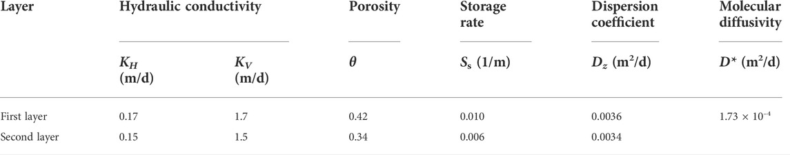
TABLE 1. The value of hydrogeological parameters.

3 Results

3.1 Field investigation

According to the building layout and production process, soil sampling (SSP) and groundwater sampling (GMW) points were set in Figure 1, where GMW2 was the monitoring point of soil and groundwater. In the later period, five soil and groundwater monitoring points (NMW) were added. The above sampling results showed that only the chloride concentration in GMW2 exceeded the standard value of class III (250 mg/L) in Chinese groundwater quality standards. In order to identify the contamination status of chloride, it is necessary to study the traceability and migration range of potential contaminant source.

Magnetotelluric method is an electromagnetic technique that uses the earth’s natural field to map the electrical resistivity changes in subsurface structures. The Magnetotelluric data is used to investigate the shallow to deep subsurface geoelectrical structures and their dimensions for the high penetration depth of the electromagnetic fields in this method (Filbandi Kashkouli et al., 2016). Thus, two geophysical methods of high density electrical method (DUK-2A MIS-60 system) and ground penetrating radar method (GSSI-SIR20 geological radar system TG1067) were used to verify the vertical distribution of strata, and the representative results are shown in Figures 2A,B and Figures 3A,B.

FIGURE 2

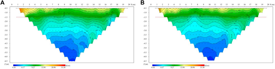
FIGURE 2. The test results of typical high density electrical method (the red dotted line represents the tested stratigraphic boundary).

FIGURE 3

FIGURE 3. The test results of typical ground penetrating radar method (the purple dotted line represents the tested stratigraphic boundary).

In Figures 2A,B, according to the apparent resistivity results, the depth within 1.5 m shows high resistance, and the apparent resistivity is 10–60 Ω▪m. The apparent resistivity changes widely, indicating that the soil in this layer is inferior in uniformity and contains impurities. It is speculated that this layer is a mixed fill soil layer. The depth below 1.5 m within the detection range shows low resistance, and the apparent resistivity is 5–10 Ω▪m. The variation range of apparent resistivity is relatively small, and the distribution of apparent resistivity in the layer is not obviously layered, which indicates that the soil quality of the layer is relatively uniform, and there is no obvious horizontal stratification of apparent resistivity distribution of artificial plain fill layer. It is inferred that the soil layer is a natural soil layer, and the water content of the soil layer is larger than that of the upper miscellaneous fill layer.

In Figures 3A,B, according to the radar detection results, the radar reflected wave intensity within the detection range is inferior, and the same axis is relatively continuous without obvious abnormal reflection, indicating that the stratum in the field is relatively uniform. From Figures 3A,B, it is clearly shown that the distribution depth of miscellaneous fill layer is less than 1.5 and 2.5 m, respectively, and the average depth of upper layer is 2 m. The clay layer is distributed below the depth of 1.5 m, and the soil is uniform. It is speculated that the soil layer is natural.

According to the detection results of high density electrical method and ground penetrating radar method, it is speculated that there are miscellaneous fill soil layers and cohesive soil layers distributed from top to bottom within the detection depth of the site. 1) The distribution depth of miscellaneous filling soil layer is within 2 m, and the soil quality of this layer is inferior and contains impurities. 2) The cohesive soil layer is distributed below the depth of 2 m, and the soil quality of this layer is relatively uniform. The apparent resistivity distribution of the artificial fill layer is characterized by obvious horizontal stratification. It is speculated that this layer is a natural soil layer, and the water content of the soil layer is larger than that of the upper miscellaneous fill layer.

The above results are based on the analysis results of high density electrical method and ground penetrating radar detection results. In addition, in order to further verify the stratigraphic characteristics, the depth of soil sampling was about 15 m in this study. The hydraulic crawler multifunctional engineering survey rig was used for drilling, the soil core was sampled and the corresponding soil samples were obtained, the process is shown in Figure 4. According to the drilling sampling analysis, the results are basically consistent with the geophysical survey results.

FIGURE 4

FIGURE 4. Drilling site and soil core sampling process.

It can be seen from Figure 5, chloride ions content curve that the values of chloride content are mainly above 400 mg/L at GMW2 sampling point, and are basically concentrated in the range of 2–10 m. The sampling curves of GMW2 and NMW2 showed the same concentration variation trend, that is, it increased with the increase of depth in the range of 0–2 m, while it decreased with the increase of depth in the range of 2–10 m, in which NMW2 is the background sampling. The imaginary line in the diagram is a traceable historical contamination curve, and the regional construction caused the inverted triangle area in the shallow range of 0–2 m. The measured concentration of the surface layer is relatively lower due to the development of the plant’s root system and microorganisms influence, in addition, the rainfall and contaminant leaching infiltrate into the surface soil after the construction disturbance.

FIGURE 5

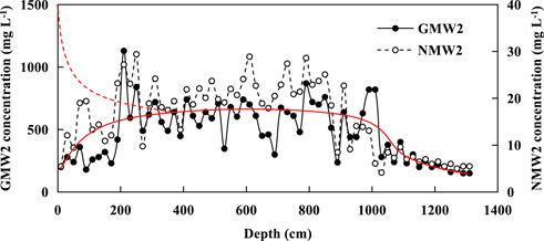
FIGURE 5. Curve diagram of measured vertical concentration change of chloride ions (the red dotted line is traceable historical contamination curve, and the red solid line is measured concentration change trend after surface disturbance).

3.2 Analytical method

In the actual site, there are six soil and groundwater monitoring points (NMW1—5 and GMW2). Due to the limitation of site scale and the monitoring results, the position of GMW2 is the center area of potential contamination sources, and vertical dispersion coefficient and vertical penetration velocity are the main parameters according to the analytical formula (8). From the field test, the value of vertical dispersion coefficient D_z is 0.0034–0.0036 m²/d. The value of vertical penetration velocity v_z is 0.015–0.017 m/d based on the observation data and model parameters calibration. Then, the z_tj of chloride is calculated by Formula (8). The calculation results are shown in Figure 6.

FIGURE 6

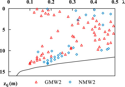
FIGURE 6. Relationship between maximum vertical migration depth (z_tj) and measured values of chloride ions under different detection criteria. (△) and (◇) represent the measured chloride ions depth of GMW2 and NMW2, respectively; The black solid line represents z_tj under different detection criteria.

Figure 6 shows that the calculation results accord with the actual situation according to two groups of chloride ions vertical concentration values, and NMW2 is used as the background value for verification. The vertical dispersion coefficient D_z is 0.0035 m²/d and the vertical penetration velocity v_z is 0.016 m/d, at this time, the source concentration value of GMW2 was about 1,500 mg/L (the measured value was 1,130 mg/L), and the z_tj was about 14 m after 720 days. Since the corresponding depths of all measured values were located within the z_tj curve of chloride ions, the calculation method proposed was effective by analytical method of z_tj.

In order to study the z_tj under different screening standards or detection standards, two typical standards were selected for comparative analysis. For example, the groundwater quality class III standard value is 250 mg/L (λ_s = 0.17) and the average chloride concentration is 600 mg/L (λ_av = 0.40) in the depth of 2–10 m range, and the calculation results are shown in Figure 7.

FIGURE 7

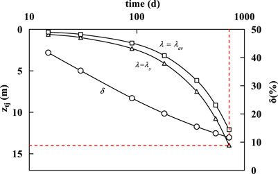
FIGURE 7. Vertical migration depth of chloride ions under different detection standards, δ is the relative deviation between λ_av and λ_s.

From Figure 7, the z_tj is about 14 m after 720 days when λ_s = 0.17, while z_tj is about 12 m when λ_av = 0.40, and the z_tj is larger by the former calculation standard, that is, the smaller the detection standard, the safer the calculation results. In addition, the relative deviation decreases with the extension of source longevity time. The relative deviation is about 10% when the source longevity time reaches 900 days. In addition, the red dotted line in Figure 7 represents the maximum penetration depth of chloride ions with the corresponding time in the actual site, which can reflect the comprehensive characteristics of the site. Therefore, in the practical application of the analytical method, it is necessary to clarify the screening standard or the detection standard, and then calculate the z_tj under different source concentrations and migration time.

3.3 Numerical method

According to the hydrogeological generalization model, the mathematical model has been adjusted and fitted to reflect the actual conditions. Since the source concentration, migration time and z_tj are determined by analytical method, six observation points (OBS1-6) have been added with the groundwater flow direction.

In order to meet the accuracy requirements of actual project, the simulation results are combined with the measured values, and the fitting result is shown in Figure 8.

FIGURE 8

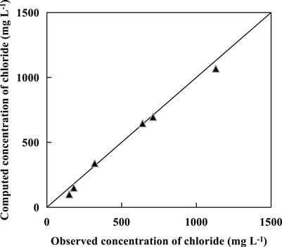
FIGURE 8. The fitting results of chloride ions measured concentration and calculated concentration.

The fitting result shows that the calculated chloride ions concentration is basically consistent with the measured value. Moreover, the plane and vertical distribution of chloride ions concentration were predicted after 720 days with GMW2 as the source center, the results are shown in Figure 9.

FIGURE 9

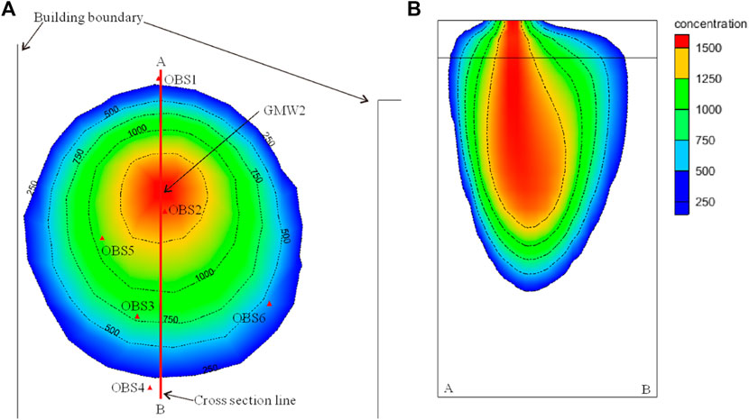
FIGURE 9. Prediction results of chloride ions concentration: (A) plane distribution; (B) vertical distribution.

From the numerical simulation results (Figure 9), the influence distance of chloride ions is about 6 m along the groundwater flow direction from the source center, the lateral distance is about 4 m, and the z_tj is about 15 m at the end of 720 days, in this condition, the groundwater quality class III standard value is used as the detection standard. The above prediction results are consistent with the measurement results, which shows that the numerical method is basically correct and can reflect the simulation process. In addition, the sources distribution characteristics can be basically reflected by arranging observation points upstream, downstream and laterally of groundwater flow direction, respectively.

4 Discussion

In the actual site, given that many decision variables are needed to be identified, two relatively simple methods are applied for the prediction of chloride migration range and duration process in source area, then the geophysical prospecting and drilling sampling analysis are also used for the verification, moreover, the source center is determined based on the difference between predicted results and measured results. Based on the above study, three main points are discussed as follows:

1) The influence of observation point layout on traceability position. The detailedness of the observed data is an important factor affecting the difficulty of solving the traceability problem (Mirghani et al., 2009). In practical applications, the number and location of observation points are restricted by construction site or costs. In order to design the appropriate number and location of observation points, it is necessary to analyze the influence of the number and location of observation points on the traceability effect. In this study, the observation points are arranged along the direction and vertical direction of groundwater flow, then the predicted results are verified by the specific observation points.

2) The influence of model parameters on traceability effect. The hydrodynamic dispersion coefficient is determined by the dispersion of medium parameters, the actual water velocity and the molecular diffusion coefficient of contaminant in the medium. Although the hydrodynamic dispersion coefficient can be obtained by experimental method, which is often determined in the process of calibration of mathematical model (Zheng and Gordon, 2009; Fetter et al., 2011), moreover, the actual average velocity affects the convection and dispersion, because the corresponding measurement error and model uncertainty will be introduced into the traceability processes (Xue, 2007). Therefore, it is necessary to consider both the measured data and the model parameter adjustment method, so as to obtain better traceability results.

3) Comparative analysis of different calculation methods. The traceability problem in the analytical method is a typical inverse problem, and the small changes of important factors will cause great differences in the calculation results. While in the simulation calculation method, the accuracy generalized model can reflect the actual solute migration, and key hydrogeological parameters determined is more important in the model calculation, therefore, it is necessary to verify the results of multiple methods.

5 Conclusion

In this paper, taking the actual site as an example, the numerical, analytical and geophysical method are used to predict and study the spatial range and diachronic process of chloride ions from source area.

The main conclusions are as follows, firstly, analytical method is simple and suitable for relatively simple hydrogeological conditions. Although the calculation results basically meet the requirements of single-point source analysis, however, for the application scope of the proposed analytical method, comparative analysis and research with existing models are required, and the error size needs to be explained in the future applications. Secondly, in the process of practical application, the traceability results are greatly affected by regional factors (groundwater flow rate, dispersion coefficient, observation point layout and concentration measurement error, etc.), and the above factors often affect the accuracy of the traceability and prediction results, thus, it is necessary to further study the parameter sensitivity in the future. Finally, the combined application of analytical method and numerical method is more conducive to the study of contamination source tracing and the range simulation. The proposed method can meet the actual situation better, and provide reference for source effective control and subsequent remediation design under the similar hydrogeological conditions.

Data availability statement

The original contributions presented in the study are included in the article/supplementary material, further inquiries can be directed to the corresponding author.

Author contributions

Conceptualization, FL and HR; methodology, JY; software, FL; validation, FL and HR; formal analysis, FL and HR; investigation, FL and HR; resources, JY and BK; data curation, FL and JY; writing—original draft preparation, FL, HR, and BK.; writing—review and editing, FL, HR, and JY; supervision, YL and YT. All authors have read and agreed to the published version of the manuscript.

Funding

This research was funded by the National Key Research and Development Program of China, grant number 2018YFC1802700; the Open Research Fund Program of State Key Laboratory of Hydroscience and Engineering, Tsinghua University, grant number sklhse-2020-D-06; the National Natural Science Foundation of China, grant number 42107162; the Natural Science Foundation of Anhui Province, grant number 1908085QD168 and the Fundamental Research Funds for the Central Universities of China, grant number PA2021 KCPY0055.

Acknowledgments

The authors would like to thank the editor and reviewers for their constructive and valuable comments and suggestions, which significantly improved the quality of this work.

Conflicts of interest

The authors declare that the research was conducted in the absence of any commercial or financial relationships that could be construed as a potential conflict of interest.

Publisher’s note

All claims expressed in this article are solely those of the authors and do not necessarily represent those of their affiliated organizations, or those of the publisher, the editors and the reviewers. Any product that may be evaluated in this article, or claim that may be made by its manufacturer, is not guaranteed or endorsed by the publisher.

References

Alexander, Y. S., Scott, L. P., and Gordon, W. W. (2006). A constrained robust least squares approach for contaminant release history identification. Water Resour. Res. 42 (4), W4414. doi:10.1029/2005wr004312

CrossRef Full Text | Google Scholar

Anna, M. M., and Peter, K. K. (2004). Application of geostatistical inverse modeling to contaminant source identification at Dover AFB, Delaware. J. Hydraulic Res. 42 (Suppl. 1), 9–18. doi:10.1080/00221680409500042

CrossRef Full Text | Google Scholar

Banaei, S., Javid, A. H., and Hassani, A. H. (2021). Numerical simulation of groundwater contaminant transport in porous media. Int. J. Environ. Sci. Technol. (Tehran). 18 (1), 151–162. doi:10.1007/s13762-020-02825-7

CrossRef Full Text | Google Scholar

Bashi-Azghadi, S. N., Kerachian, R., Bazargan-Lari, M. R., and Solouki, K. (2010). Characterizing an unknown pollution source in groundwater resources systems using PSVM and PNN. Expert Syst. Appl. 37 (10), 7154–7161. doi:10.1016/j.eswa.2010.04.019

CrossRef Full Text | Google Scholar

Chakraborty, A., and Prakash, O. (2020). Identification of clandestine groundwater pollution sources using heuristics optimization algorithms: A comparison between simulated annealing and particle swarm optimization. Environ. Monit. Assess. 192 (12), 791–819. doi:10.1007/s10661-020-08691-7

PubMed Abstract | CrossRef Full Text | Google Scholar

Chen, Y. M., Xie, H. J., and Zhang, C. H. (2016). Review on penetration of barriers by contaminants and technologies for groundwater and soil contamination control. Adv. Sci. Technol. Water Resour. 36 (01), 1–10.

Google Scholar

Ellen, M., and Pierre, P. (2007). Simultaneous identification of a single pollution point-source location and contamination time under known flow field conditions. Adv. Water Resour. 30 (12), 2439–2446. doi:10.1016/j.advwatres.2007.05.013

CrossRef Full Text | Google Scholar

Fetter, C. W., Fei, T., Zhou, N. Q., et al. (2011). Contaminant hydrogeology. Beijing, China: Higher Education Press.

Google Scholar

Filbandi Kashkouli, M., Kamkar Rouhani, A., Moradzadeh, A., et al. (2016). Dimensionality analysis of subsurface structures in magnetotellurics using different methods (a case study: Oil field in southwest of Iran). J. Min. Environ. 7 (1), 119–126.

Google Scholar

Gongsheng, L., Tan, Y. J., Cheng, J., and Wang, X. Q. (2006). Determining magnitude of groundwater pollution sources by data compatibility analysis. Inverse Problems Sci. Eng. 14 (3), 287–300. doi:10.1080/17415970500485153,

CrossRef Full Text | Google Scholar

Gurarslan, G., and Karahan, H. (2015). Solving inverse problems of groundwater-pollution-source identification using a differential evolution algorithm. Hydrogeol. J. 23 (6), 1109–1119. doi:10.1007/s10040-015-1256-z

CrossRef Full Text | Google Scholar

Ilaria, B., and Maria, G. T. (2003). A geostatistical approach to recover the release history of groundwater pollutants. Water Resour. Res. 39 (12), 1372. doi:10.1029/2003wr002314

CrossRef Full Text | Google Scholar

Ilaria, B., Maria, G. T., and Andrea, Z. (2012). Simultaneous identification of the pollutant release history and the source location in groundwater by means of a geostatistical approach. Stoch. Environ. Res. Risk Assess. 27 (5), 1269–1280. doi:10.1007/s00477-012-0662-1

CrossRef Full Text | Google Scholar

Jordi, G., and Yoram, C. (1996). Contaminant migration in the unsaturated soil zone: The effect of rainfall and evapotranspiration. J. Contam. Hydrology 23 (3), 185–211. doi:10.1016/0169-7722(95)00086-0

CrossRef Full Text | Google Scholar

Juliana, A., and Amvrossios, C. B. (2001). State of the art report on mathematical methods for groundwater pollution source identification. Environ. Forensics 2 (3), 205–214. doi:10.1006/enfo.2001.0055

CrossRef Full Text | Google Scholar

Lapworth, D. J., Baran, N., Stuart, M. E., and Ward, R. (2012). Emerging organic contaminants in groundwater: A review of sources, fate and occurrence. Environ. Pollut. 163 (Apr), 287–303. doi:10.1016/j.envpol.2011.12.034

CrossRef Full Text | Google Scholar

Li, J. L., Long, Y. Q., and Wu, C. Y. (2017). A groundwater pollution source identification method based on the simple genetic algorithm. Adv. Environ. Prot. 7 (01), 35–40. doi:10.12677/aep.2017.71005

CrossRef Full Text | Google Scholar

Liu, J. B., Jiang, S. M., Zhou, N. Q., et al. (2021). Groundwater contaminant source identification based on QS-ILUES. J. Groundw. Sci. Eng. 9 (1), 73–82. doi:10.19637/j.cnki.2305-7068.2021.01.007

CrossRef Full Text | Google Scholar

Long, Y. Q., Wu, C. Y., and Wang, J. P. (2014). The influence of estimated pollution range on the groundwater pollution source identification method based on the simple genetic algorithm. Appl. Mech. Mater. 3308, 836–841. doi:10.4028/www.scientific.net/amm.587-589.836

CrossRef Full Text | Google Scholar

Mahar, P. S., and Datta, B. (1997). Optimal monitoring network and groundwater-pollution source identification. J. Water Resour. Plan. Manag. 123 (4), 199–207. doi:10.1061/(asce)0733-9496(1997)123:4(199)

CrossRef Full Text | Google Scholar

Mahsa, A., and Bithin, D. (2013). Identification of contaminant source characteristics and monitoring network design in groundwater aquifers: An overview. J. Environ. Prot. (Irvine, Calif. 4 (5A), 26–41. doi:10.4236/jep.2013.45a004

CrossRef Full Text | Google Scholar

Mangold, D. C., and Tsang, C. F. (1991). A summary of subsurface hydrological and hydrochemical models. Rev. Geophys. 29 (1), 51–79. doi:10.1029/90rg01715

CrossRef Full Text | Google Scholar

Manish, J., and Bithin, D. (2013). Three-dimensional groundwater contamination source identification using adaptive simulated annealing. J. Hydrol. Eng. 18 (3), 307–317. doi:10.1061/(asce)he.1943-5584.0000624

CrossRef Full Text | Google Scholar

Mark, F. S., and Peter, K. K. (1997). A geostatistical approach to contaminant source identification. Water Resour. Res. 33 (4), 537–546. doi:10.1029/96wr03753

CrossRef Full Text | Google Scholar

Mirghani, B. Y., Mahinthakumar, K. G., Tryby, M. E., Ranjithan, R. S., and Zechman, E. M. (2009). A parallel evolutionary strategy based simulation–optimization approach for solving groundwater source identification problems. Adv. Water Resour. 32 (9), 1373–1385. doi:10.1016/j.advwatres.2009.06.001

CrossRef Full Text | Google Scholar

Nigro, A., Sappa, G., and Barbieri, M. (2017). Application of boron and tritium isotopes for tracing landfill contamination in groundwater. J. Geochem. Explor. 172, 101–108. doi:10.1016/j.gexplo.2016.10.011

CrossRef Full Text | Google Scholar

Palau, J., Marchesi, M., Chambon, J. C., Aravena, R., Canals, A., Binning, P. J., et al. (2014). Multi-isotope (carbon and chlorine) analysis for fingerprinting and site characterization at a fractured bedrock aquifer contaminated by chlorinated ethenes. Sci. total Environ. 475, 61–70. doi:10.1016/j.scitotenv.2013.12.059

PubMed Abstract | CrossRef Full Text | Google Scholar

Rashid, A., Khattak, S. A., Ali, L., Zaib, M., Jehan, S., Ayub, M., et al. (2019). Geochemical profile and source identification of surface and groundwater pollution of District Chitral, Northern Pakistan. Microchem. J. 145, 1058–1065. doi:10.1016/j.microc.2018.12.025

CrossRef Full Text | Google Scholar

Shi, S., Wei, Z., Shengwei, W., Ng, C. W. W., Chen, Y., and Chiu, A. C. F. (2018). Leachate breakthrough mechanism and key pollutant indicator of municipal solid waste landfill barrier systems: Centrifuge and numerical modeling approach. Sci. Total Environ. 612, 1123–1131. doi:10.1016/j.scitotenv.2017.08.185

CrossRef Full Text | Google Scholar

Song, K., Ren, X., Mohamed, A. K., Liu, J., and Wang, F. (2020). Research on drinking-groundwater source safety management based on numerical simulation. Sci. Rep. 10 (1), 15481–15517. doi:10.1038/s41598-020-72520-7

CrossRef Full Text | Google Scholar

Sturchio, N. C., Beloso, A., Heraty, L. J., Wheatcraft, S., and Schumer, R. (2014). Isotopic tracing of perchlorate sources in groundwater from Pomona, California. Appl. Geochem. 43, 80–87. doi:10.1016/j.apgeochem.2014.01.012

CrossRef Full Text | Google Scholar

Subba Rao, N. (2006). Seasonal variation of groundwater quality in a part of Guntur District, Andhra Pradesh, India. Environ. Geol. 49 (3), 413–429. doi:10.1007/s00254-005-0089-9

CrossRef Full Text | Google Scholar

Wang, H., and Zhang, Q. (2019). Research advances in identifying sulfate contamination sources of water environment by using stable isotopes. Int. J. Environ. Res. Public Health 16, 1914. doi:10.3390/ijerph16111914

PubMed Abstract | CrossRef Full Text | Google Scholar

Wu, J. C., Xue, Y. Q., Zhang, Z. H., et al. (1997). Numerical simulation of groundwater pollution in Taiyuan basin. J. Nanjing Univ. Nat. Sci. 33 (3), 70–79.

Google Scholar

Xiao, C. N., Lu, W. X., Zhao, Y., et al. (2016). Optimization method of identification of groundwater pollution sources based on radial basis function model. China Environ. Sci. 36 (7), 2067–2072.

Google Scholar

Xue, Y. Q. (2007). Groundwater numerical simulation. Beijing, China: Science Press.

Google Scholar

Xue, Y. Q. (2010). Present situation and prospect of groundwater numerical simulation in China. Geol. J. China Univ. 16 (01), 1–6.

Google Scholar

Yu, Q. L., Wei, L., and Ju, H. (2012). Advance of optimization methods for identifing groundwater pollution source porperties. Appl. Mech. Mater. 1802, 603–608. doi:10.4028/www.scientific.net/amm.178-181.603

CrossRef Full Text | Google Scholar

Zheng, C. M., and Gordon, G. B. (2009). Applied contaminant transport modeling. Beijing, China: Higher Education Press.

Google Scholar

Zhu, X. Y., and Liu, J. L. (2001). Numerical study of contaminants transport in fracture-karst water in Dawu well field, Zibo city, Shandong province. Earth Science Frontiers. Beijing: China University of Geosciences, 171–178.01

Google Scholar

Zimmermann, J., Halloran, L. J., and Hunkeler, D. (2020). Tracking chlorinated contaminants in the subsurface using compound-specific chlorine isotope analysis: A review of principles, current challenges and applications. Chemosphere 244, 125476. doi:10.1016/j.chemosphere.2019.125476

PubMed Abstract | CrossRef Full Text | Google Scholar

Zoi, D., and George, F. P. (2009). Optimal search strategy for the definition of a DNAPL source. J. Hydrology 376 (3), 542–556. doi:10.1016/j.jhydrol.2009.07.062

CrossRef Full Text | Google Scholar