Refined machine learning modeling of reservoir discharge water temperature

1 Introduction

China has the world’s largest installed capacity of hydropower, which contributes over 60% of the country’s renewable energy supply (Ge et al., 2023). Hydroelectric power, as a clean energy source, can reduce carbon emissions while meeting energy needs (Li and Zhang, 2014). However, reservoir construction may cause a series of adverse environmental impacts (Zhang et al., 2022; Lu et al., 2023). After the construction of a reservoir, thermal stratification can occur in the water body, causing the discharge water temperature (DWT) to deviate from the natural water temperature (Ren et al., 2019). Due to the crucial role of water temperature in water quality and aquatic ecosystem processes (Booker and Whitehead, 2022), DWT fluctuations may have adverse effects on downstream aquatic ecosystems (Lu et al., 2023). Therefore, DWT prediction and control is currently a topic of concern for reservoir managers. To protect downstream ecological health as much as possible, there is an urgent need to establish an efficient and accurate DWT prediction model for reservoir water temperature management.

The commonly used methods for studying the DWT include prototype observations (Gray et al., 2019), physical model experiments (Song et al., 2020), and numerical simulation (He et al., 2018) methods. The prototype observation method is the most direct method for obtaining DWT data. This method is the foundation for thermal analysis, numerical simulation, and other related fields. The physical model experiment method is based on a simulation of the temperature and flow fields of a reservoir by a model. This method explores the relationship between the DWT and influencing factors based on different operating conditions. Establishing empirical formulas based on the patterns of prototype observation and physical model experiment data can be applied to achieve rapid DWT prediction (Gao et al., 2014). However, these formulas are based on fitting the relationship between existing data, and there is no complete theoretical derivation process. In practical applications, there is significant uncertainty, and accuracy is difficult to guarantee. The numerical simulation method is based on physical mechanisms, and existing one-dimensional models, such as GLM-ADE (Weber, 2018), two-dimensional models, such as CE-QUAL-W2 (Larabi et al., 2022), and three-dimensional models, such as Flow-3D (He et al., 2018) can effectively calculate the DWT. However, the numerical simulation calculation time is relatively long, and due to the need for multiple scheme decisions in a short period in actual management scenarios, it is not suitable for timely DWT prediction. Therefore, it is difficult to meet the needs of efficiently and accurately predicting the DWT simultaneously to provide a decision-making basis for managers with commonly used methods.

Flexible and efficient machine learning (ML) algorithms have been applied to water temperature prediction (Zhu and Piotrowski, 2020). Fewer input variables are needed in ML models than in numerical simulation methods. Moreover, ML models have similar or even better performance than numerical simulation methods (Zhang et al., 2022). In addition, it is more convenient to combine ML models with optimization algorithms, helping managers make efficient optimization decisions (Wang et al., 2022). At present, ML algorithms are mainly applied to predict river water temperature at different time scales. For example, Sivri et al. (2009) successfully predicted monthly stream water temperature using an artificial neural network (ANN) model, while Zhu et al. (2019) constructed a daily scale river water temperature prediction model using an extreme learning machine (ELM) model. In addition, Lu and Ma (2020) conducted ML modeling for hourly scale river water temperature. However, due to the much more complex thermal state of reservoirs compared to that of rivers, research on ML modeling of reservoir water temperature is currently relatively limited. Soleimani et al. (2016) constructed a DWT prediction model using multilevel water intake data based on a support vector machine (SVM). Lu et al. (2023) and Zhang et al. (2022) constructed DWT prediction models using stratified water intake data from a stacked beam gate based on support vector regression (SVR) and long short-term memory (LSTM), respectively. In most existing research, the daily scale DWT is modeled. As automatic water temperature monitoring equipment has become popular, hourly scale DWT datasets have begun to contain rich data. Furthermore, due to diurnal changes in meteorological conditions, diurnal changes in water temperature may be significant (Yang et al., 2020). As researchers pay increasingly more attention to the impact of reservoir water temperature on downstream water ecology, it is essential to accurately and efficiently predict the DWT on an hourly scale.

In summary, the main objective of this study is to construct a ML prediction model for hourly scale DWT, enabling more efficient and refined reservoir management. In this study, the Pubugou Reservoir (PBGR) in southwestern China is selected as an example. To obtain a better ML model, the modeling performance of SVR, linear regression (LR), K-nearest neighbor (KNN), random forest regressor (RFR), gradient boost regression tree (GBRT), and multilayer perceptron neural network (MLPNN) in terms of hourly scale DWT is compared. Finally, the hourly scale early warning performance of the optimal model and the ability to optimize the scheduling of DWT are explored.

2 Materials and methods

2.1 Study area and data sources

In this study, the PBGR on the Dadu River Basin in southwestern China is selected as an example. The PBGR, the 19th level of the planned cascade of the main stream of the Dadu River, is a controlling reservoir in the middle reaches of the Dadu River and has seasonal regulation capacity. The PBGR is mainly used for power generation and has other functions, such as sediment retention and flood control. The maximum dam height of the PBGR is 186 m, and the total installed capacity is 3600 MW. The total storage capacity of the PBGR is 53.37 × 10⁸ m³. The reservoir area is 84.14 km², and the backwater length is approximately 72 km (Zhang and Xu, 2014). Statistics have shown that there are various types of protected Chinese fish species distributed in the Dadu River Basin (Bangfu et al., 2022). The water temperature discharged from the reservoir may have adverse effects on these protected fish species (Zhou et al., 2016). Therefore, this study focuses on the DWT of the PBGR, a large reservoir in the Dadu River Basin.

We conducted a water temperature prototype observation at the PBGR in 2022, automatically monitoring the reservoir vertical water temperature (RVWT) and DWT. The monitoring points are shown in Figure 1. A temperature chain was installed approximately 800 m upstream of the PBGR dam to monitor the RVWT, with a monitoring frequency of once per hour. Eighteen thermometers were tied to the temperature chain. We installed temperature recorders at depths of 0.5 m, 1–10 m (1 every 1 m) and 20–80 m (1 every 10 m). The DWT monitoring frequency is also once per hour. In addition, we obtained reservoir operation data on water level (WL) and discharge flow (DF) data from the dam management office, with a frequency of once per hour. All types of data were recorded at the same time, and the monitoring data were organized. A total of 5,288 sets of valid data were obtained (due to equipment failures during some periods, corresponding data were removed).

FIGURE 1

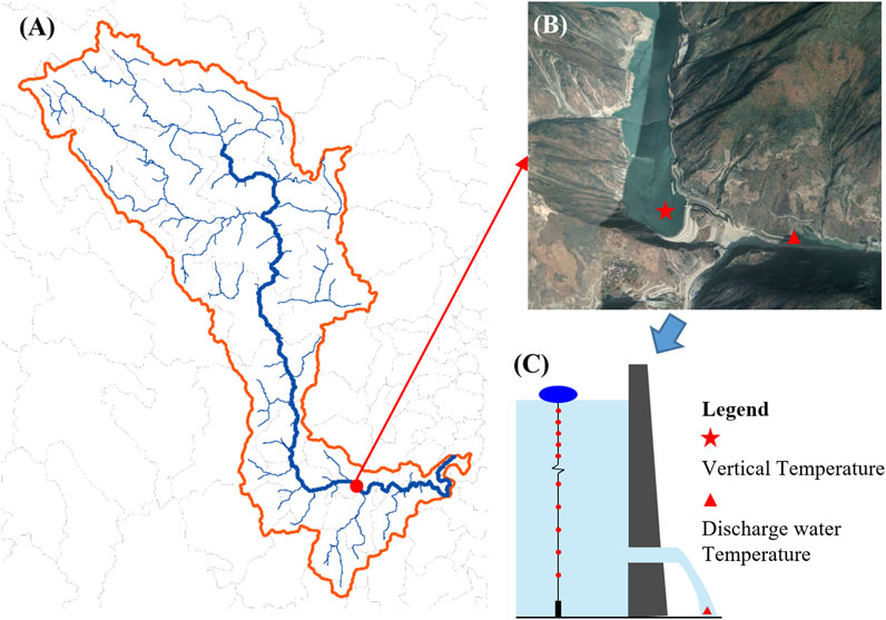
FIGURE 1. Location and monitoring points of the PBGR. (A) Dadu river basin; (B) Area in front of the PBGR Dam; (C) Schematic diagram of water temperature monitoring.

2.2 Modeling and model application process

Figure 2 shows the flowchart for modeling and model application. The step 1 is to select indicators. Firstly, since the DWT is the target of our prediction, it has been chosen as the output. Then, the input indicators of the model are selected according to the impact mechanism of the DWT. At last, the corresponding data are collected and integrated to construct a dataset. The step 2 is to establish the DWT ML prediction models. In this step, the data are first preprocessed to satisfy the requirements of the ML algorithms. The preprocessing steps include dividing the dataset into training, validation, and test sets, as well as standardizing the data. Then, different ML algorithms are selected for comparison, and the most suitable algorithm is selected for DWT prediction. The algorithms selected in this study include SVR, KNN, MLPNN, LR, RFR, and GBRT, all of which are implemented in Python. Then, the optimization algorithms are used to optimize the model parameters during the training process to build the optimal parameter prediction model. The step 3 is to input the test set data into the optimal parameter prediction model for calculation. The model is then evaluated by combining the predicted and measured values that are output from the model to obtain the most suitable ML algorithm for the DWT prediction of the case reservoir. The step 4 is to apply the optimal model selected in the step 3. Among them, the step 4.1 builds an early warning model, and the step 4.2 optimizes the scheduling of DWT. In the step 4.1, the previous model achieves real-time outputs based on real-time inputs. However, this model is not suitable for reservoir managers to make management decisions. Therefore, we build an early warning model based on the DWT and input values n hours ago, repeating steps 2 and 3 to build a model that is suitable for managers’ decisions. In step 4.2, we select typical thermal stratification days and adjust the DWT of the reservoir by adjusting the DF in hydrological conditions to determine the most suitable DF pattern.

FIGURE 2

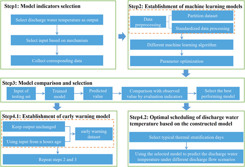
FIGURE 2. Flowchart for modeling and model application.

2.3 Model indicator selection

ML models are black box models that do not consider physical processes. Therefore, the performance and generalizability of the model largely depend on its input and output (Zhang et al., 2022). Therefore, selecting input indicators based on the impact mechanism of the DWT will help to increase the interpretability of the model. Some studies have investigated the factors influencing the DWT in reservoirs based on numerical simulations and experiments (He et al., 2018; Yang et al., 2021; Liu et al., 2022). The results of these studies indicate that the DWT is related to the RVWT, WL, and DF.

Deep reservoirs often experience thermal stratification, especially during high temperature seasons. As shown in Figure 3, when the reservoir is in the thermal stratification period, the difference in RVWT will generate buoyancy to hinder the vertical movement of the water body. The size of the DF determines whether the inertial force generated by the DF can suppress buoyancy, further determining where the discharge comes from. When the DF is small, the buoyancy effect is sufficient to hinder the vertical movement of the water body, and the water intake can only reach the water near it (Figure 3, blue dashed line); As the DF increases, the inertial force will gradually suppress the buoyancy effect, and the water intake can take water closer to the surface (Figure 3, red dashed line). In addition, the changes in WL affect the water head and the distribution of RVWT, thus also having a significant impact on the DWT. Figure 3 generalizes the flow pattern, and in fact, there are complex mixed flows in the reservoir, including inflow mixing, surface mixing, internal mixing, etc (Zhang et al., 2022). However, when we use factors close to the front of the dam as input indicators, we can minimize the impact of complex mixing processes on the results. To sum up, the RVWT, DF, and WL are selected as the input indicators for the ML models in this study, and the mathematical expression of the DWT prediction model in this study is shown in Equation 1.

$\text{DWT}=\mathrm{f}\left(RVWT,WL,DF\right)(1)$

FIGURE 3

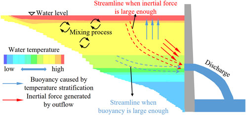
FIGURE 3. Brief schematic diagram of water intake flow pattern.

2.4 Machine learning modeling process

2.4.1 Machine learning algorithms

We examined the DWT prediction performance of six ML algorithms, SVR, KNN, MLPNN, LR, RFR, and GBRT, using the sklearn library in Python. These six algorithms are introduced below.

2.4.1.1 SVR

SVR is an application model of SVM in regression problems. The main idea of SVR is to find a hyperplane in a feature space, minimizing the distance between the hyperplane and the training samples while also meeting a certain tolerance (i.e., allowing some training samples to exceed a certain distance range) (Wang et al., 2022). This distance is usually calculated using a “kernel function”, which enables SVR to perform well in nonlinear problems. Due to the different performances of different kernel functions, we investigated the performance of ML models using linear functions, polynomial functions, radial basis functions (RBF), and sigmoid functions. In addition, the parameters of the SVR model, mainly the penalty coefficient C and kernel function coefficient γ, have a significant impact on the model performance.

2.4.1.2 KNN

The KNN algorithm is a nonparametric classification and regression method that is commonly used in pattern recognition and ML. The basic idea of the KNN algorithm is to determine the classification or prediction value of an unlabeled data point by measuring the distances between data points (Guo et al., 2006). The KNN algorithm does not require explicit model training during the training phase. Instead, it draws inferences from existing data during the prediction phase. The advantages of the KNN algorithm include its simplicity and applicability to multiclass problems. In addition, the KNN algorithm makes no assumptions about the data distribution. However, it also has some drawbacks, including its high computational overhead (i.e., it requires distance calculations between all training samples), sensitivity to outliers, and so on. When using the KNN algorithm, it is usually necessary to consider issues such as the selection of K-values and distance metrics to achieve better prediction performance. Common distance measures include the Euclidean distance, Manhattan distance, etc.

2.4.1.3 MLPNN

The MLPNN is a common artificial neural network used for various ML tasks, such as classification and regression (Velasco et al., 2019). It consists of multiple layers, each containing multiple neurons. The MLPNN typically consists of an input layer, a hidden layer, and an output layer. The input layer receives raw data or features and passes them to the hidden layer. The hidden layer is the core of a neural network, which can have one or more hidden layers. Each hidden layer can contain multiple neurons. Each neuron is connected to all neurons in the previous layer, and each connection has a weight value that can be adjusted according to the training data. The function of the hidden layer is to perform nonlinear transformations on the input data, enabling the neural network to learn more complicated patterns. Finally, the output layer generates the results of the neural network. We adopted the simplest MLPNN model structure, which consists of one input layer, one output layer, and some hidden layers. The number of hidden layer neurons is an important parameter that is determined by parameter optimization.

2.4.1.4 LR

LR is a common statistical and ML method used to establish models of linear relationships between variables. In LR, an attempt is made to predict the relationship between a dependent variable (or response variable) and one or more independent variables (or features) by fitting a straight line. By finding the optimal slope and intercept, the most suitable linear relationship among the data points can be established for prediction or analysis.

2.4.1.5 RFR

RFR is a ML algorithm that uses an ensemble learning method (Alwadai et al., 2022). Ensemble learning is a technique that combines multiple models to achieve better prediction performance. RFR is an improved random forest algorithm for regression problems. In regression problems, the goal is to predict a continuous numerical output, rather than discrete labels as in classification problems. RFR makes predictions by combining multiple decision tree models trained on different datasets. It also performs well in handling high-dimensional data, missing values, and outliers. In summary, RFR is a powerful ML algorithm that can be used to solve various regression problems.

2.4.1.6 GBRT

The GBRT is a powerful ML technique used to solve regression problems (Xu et al., 2023). It is a type of ensemble learning method that improves the prediction performance by combining multiple decision tree models. Specifically, the working method of the GBRT is to gradually construct a series of decision tree models, each of which is trained based on the residuals of the previous model. During the training process, the model pays more attention to samples with previous model prediction errors to gradually reduce the overall prediction error. This is achieved by adjusting the weights of the samples and the learning rate, allowing each new model to focus more on samples that the previous model did not predict correctly.

2.4.2 Preprocessing before modeling

The dataset was stochastically divided into training, validation, and test sets with the widely accepted ratio of approximately 6:2:2 (Yoon, 2021). A total of 3,174 training set data were used to train the model, 1,058 validation set data were used for parameter optimization, and 1,056 test set data were used to test the model’s generalizability and robustness. In addition, to avoid the impact of differences in data magnitude on the model’s learning ability, Eq. 2 was applied to standardize the data.

${\mathrm{X}}_i^{\prime }=\frac{X_i-\overline{X}}{\sigma }(2)$

Where $X_i$ is the original sample value, $\overline{X}$ is the average value of the original sample, $\sigma$ is the standard deviation of the original sample, and ${\mathrm{X}}_i^{\prime }$ is the standardized value.

2.4.3 Parameter optimization

The genetic algorithm is a popular parameter optimization algorithm that has been applied in multiple ML model research (Wang et al., 2022; Quan et al., 2022). This algorithm is designed and proposed based on the evolutionary laws of organisms in nature. When optimizing parameters, genetic algorithms usually first construct a set of random solutions called populations and evaluate these solutions through fitness functions. Then, leave behind some solutions with higher fitness, and generate the next-generation through crossover and mutation. In this way, as the algebra increases, the solution develops towards the optimal direction until it reaches the stopping condition. Finally, the genetic algorithm will output the solution with the highest fitness, which is the approximate optimal solution of the problem. Therefore, when setting the algorithm, it is necessary to set the fitness function, population size, maximum genetic algebra, crossover fraction, and mutation fraction. When using genetic algorithms to solve complex combinatorial optimization problems, better optimization results are achieved more quickly compared to those of some conventional optimization algorithms.

2.4.4 Model performance evaluation methods

Three evaluation indicators, the root mean square error (RMSE), mean absolute error (MAE), and Nash–Sutcliffe efficiency (NSE), were used to evaluate the performance of the model. When the RMSE and MAE values are smaller and the NSE is closer to 1, the prediction performance of the model is better (Lu et al., 2023). The calculation formulas for the evaluation indicators are as follows:

$\text{RMSE}=\sqrt{\frac{1}{n}{\displaystyle \sum _{i=1}^n}{\left({ob}_i-{\mathit{pr}}_i\right)}^2}(3)$

$\text{MAE}=\frac{1}{n}{\displaystyle \sum _{i=1}^n}\left|{ob}_i-{\mathit{pr}}_i\right|(4)$

$\text{NSE}=1-\frac{{\sum }_{i=1}^n{\left({ob}_i-{\mathit{pr}}_i\right)}^2}{{\sum }_{i=1}^n{\left({ob}_i-\overline{ob}\right)}^2}(5)$

where $n$ is the sample size, ${ob}_i$ and ${\mathit{pr}}_i$ are the monitored and predicted values of the ith sample, respectively, and $\overline{ob}$ is the average of the monitored values.

3 Results and discussion

3.1 Analysis of discharge water temperature

In addition to the DWT in 2022 (DWT 2022) monitored in this study, we also collected the natural water temperature at the dam site before the construction of the PBGR, the discharge water temperature in 2017 (DWT 2017), and the DWT in 2018 (DWT 2018). We processed these water temperature data into monthly averages and displayed them in Figure 4. Affected by meteorological conditions, the natural water temperature showed a trend of increasing from January to August and decreasing from August to December. The construction of the reservoir had a certain impact on the rhythm of water temperature, showing a consistent pattern in DWT 2017, DWT 2018, and DWT 2022, namely, a decrease from January to March, an increase from March to September, and a decrease from September to December. Compared to natural water temperatures, the PBGR released low temperature water from March to August and high temperature water from other months. It can be seen that the construction of the PBGR has disrupted the rhythm of natural water temperature, which is consistent with many existing reservoirs (Alavian et al., 1992; Lu et al., 2023; Wang et al., 2024). Within the statistical year (Figure 4), the maximum low-temperature water discharge amplitude is 2.9°C, which will have a negative impact on the aquatic ecology downstream of the dam (Zhang et al., 2015; Labaj et al., 2016). As the watershed where the study case is located, the Dadu River Basin is home to numerous habitats and spawning grounds for protected Chinese fish species (Song et al., 2008; Bangfu et al., 2022). Numerous reservoirs have been constructed in the Dadu River Basin, disrupting the natural fluctuations of the water temperature and potentially threatening the survival and reproduction of fish (Barbarossa et al., 2021). Therefore, how to achieve rapid prediction and regulation of watershed water temperature is an urgent problem to be solved.

FIGURE 4

FIGURE 4. Discharge water temperature of PBGR in different periods.

3.2 Construction of machine learning models for discharge water temperature

3.2.1 Parameter optimization based on genetic algorithm

The genetic algorithm was used to optimize the parameters of the models. We referred to (Wang et al., 2022) to set the parameters of the genetic algorithm (Table 1) and used R² as the fitness function. When using the coefficient of determination (R²) as the fitness function of the genetic algorithm, the larger the R² value is, the better the model performance. The optimal parameters and their R² values on the validation set are presented in Table 2. In response to the problem in this study, the SVR algorithm performs best when using RBF as the kernel function. The optimal values for C and γ are 15.4 and 0.58, respectively, corresponding to an R² of 0.979. When using the KNN to model, the optimal number of neighbors is determined to be 5, and with this setting, the R² is 0.945. When using the MLPNN model for prediction, the optimal results are obtained when using the tanh function as the activation function. With this setting, the use of 761 hidden layers is optimal, and the corresponding R² is 0.941. The performance of the LR model is poor, with an R² of only 0.862. However, the performance of the RFR and GBRT is similar to that of SVR. The optimal results are achieved with these two models when using 22 decision trees and 89 decision trees, respectively, with corresponding R² values of 0.962 and 0.967. It can be seen that during the training process, the optimal model is the SVR model, followed by the GBRT and RFR models. This study used genetic algorithm for parameter optimization to quickly obtain high-precision models. We also attempted grid search and found that the efficiency of the same parameter range was much lower than that of genetic algorithms. Some studies (Liashchynskyi and Liashchynskyi, 2019; Alibrahim and Ludwig, 2021) have pointed out that the performance of different optimization algorithms is difficult to compare. However, for larger parameter search ranges, evolutionary algorithms such as genetic algorithms are the best options for parameter optimization. Therefore, when we do not know the approximate position of the parameters, in order to obtain the optimal parameter combination, genetic algorithms can be used to obtain the desired results most efficiently.

TABLE 1

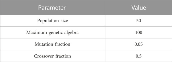
TABLE 1. Genetic algorithm parameter settings (Wang et al., 2022).

TABLE 2

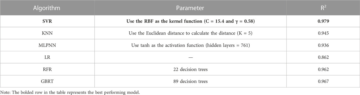
TABLE 2. Optimal parameters and validation stage performance for each model.

3.2.2 Comparison and selection of models

In this section, the model performance of the six ML algorithms with their best settings, as obtained in Section 3.2.1, is evaluated. In addition, the prediction performance of each model is evaluated using the fitting effect between the observed and predicted values, as well as the MAE, RMSE, and NSE statistical indicators.

Figure 5 shows the prediction results of the optimal settings of the six models on the test set. The fitting effects of most models are within the acceptance range. The R² values of the SVR, KNN, MLPNN, LR, RFR, and GBRT models are 0.976, 0.972, 0.908, 0.875, 0.974, and 0.976, respectively. From the model performance evaluation indicators in Table 3, the performance of the SVR model is superior to that of the other models. The RMSE, MAE, and NSE values of the SVR model are 0.490°C, 0.272°C, and 0.976, respectively, while those of the KNN model are 0.530°C, 0.226°C, and 0.972, respectively. The RMSE and MAE values of the MLPNN model were significantly higher than those of SVR and KNN, with values of 0.969 °C and 0.570°C, respectively. Thus, the performance of this model is clearly unsatisfactory. The RMSE, MAE, and NSE values of the LR are 1.137°C, 0.706°C, and 0.871, respectively, indicating that the problem of DWT is a nonlinear problem. The performance of the RFR and GBRT models is similar but still slightly inferior to that of the SVR model. The maximum absolute error of each model was statistically analyzed, and the values of the SVR, KNN, MLPNN, LR, RFR, and GBRT models are 3.76°C, 5.10°C, 8.10°C, 9.78°C, 8.74°C, and 3.99°C, respectively. In addition, when comparing the models in terms of the validation and test set results, the SVR, and GBRT models all show similar performance. However, the SVR model is more stable, with the smallest R² difference between the validation and test sets. Overall, we evaluated the performance of the models from multiple perspectives. The maximum absolute errors of the KNN, LR, RFR, and MLPNN were unacceptable, even if the overall errors of some models were small. Therefore, these four models were excluded, and the performance rankings of the other models were as follows: SVR > GBRT. Hence the SVR model (RBF kernel function) was chosen as the DWT prediction model, which is consistent with previous research (Lu et al., 2023).

FIGURE 5

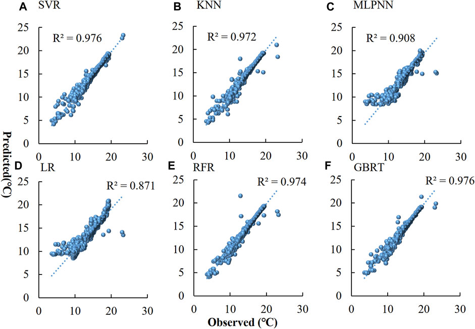
FIGURE 5. Scatter plot of DWT observed and predicted in the test set. (A–F) Represent the results of SVR, KNN, MLPNN, LR, RFR, and GBRT models, respectively.

TABLE 3

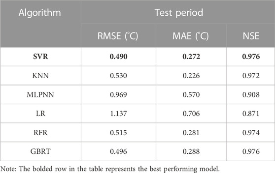
TABLE 3. Model performance evaluation index values during the test period.

We compared the DWT prediction performance of six ML models, namely, the SVR, LR, RFR, KNN, MLPNN, and GBRT models. Among them, the LR model has the worst performance (Table 2; Table 3; Figure 5). The DWT problem is a nonlinear problem. Thus, the LR model has poor mechanism recognition. The other models are able to better identify DWT variations (Table 2; Table 3; Figure 5), among which the SVR model (RBF kernel function) has the best performance. ML algorithms have the ability to make functional predictions by establishing mapping relationships between input and output indicators. The SVR model has a good nonlinear relationship modeling ability, mapping data to higher dimensional spaces through kernel functions, thereby finding better linear relationships in new spaces (Meng et al., 2023). In addition, RBF kernel functions have strong nonlinear modeling capabilities, mapping data to high-dimensional spaces, enabling better identification of nonlinear relationships in new spaces and capturing more complex data patterns. The shape of the RBF kernel function can be adaptively adjusted according to the data distribution, thereby improving the flexibility of the model. In this study, the SVR model using RBF is the most suitable for predicting the DWT of the case reservoir. However, it should be noted that the performance differences of the various models in this study are not significant. Therefore, the optimal algorithm should be redefined when applied to other reservoirs.

3.3 Early warning model performance

We used the SVR model with the best performance in section 3.2 to construct a DWT early warning model. This model was refined based on an hourly scale. The early warning hours ranged from 1 h to 24 h. Train and test warning models at different times, and conduct statistical analysis of model performance (Figure 6). Overall, the performance of nonearly warning model (0 h) is slightly better than that of early warning models (1 h–24 h). The RMSE and MAE values of the early warning model (1 h–24 h) are slightly higher than those of the nonearly warning model (0 h) while the R² is slightly lower. The R² of the early warning models fluctuate in the range of 0.943–0.979 for 1 h–24 h, while the RMSE and MAE values fluctuate in the range of 0.487°C–0.604°C and 0.222 °C–0.305°C, respectively. The performance is acceptable, and the model can provide early warning functions within 24 h.

FIGURE 6

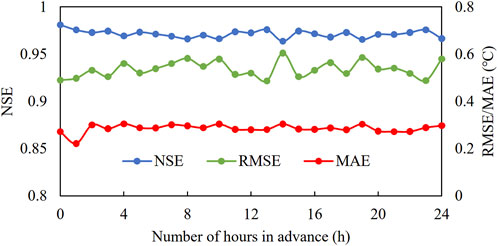
FIGURE 6. Early warning model performance.

At present, researchers have proposed many ML prediction models for river water temperature (Zhu and Piotrowski, 2020; Jiang et al., 2022), but there are few warning models and almost no research on hourly scale warning models for reservoir DWT. For the river water temperature, its natural value, which is not affected by the reservoir, fluctuates with air temperature during the day (Hebert et al., 2014; Croghan et al., 2019). However, under the influence of the reservoir, the downstream water temperature flattens (Yong-Bo et al., 2010). To best mitigate the impact of the reservoir on downstream water temperature, the DWT should be adjusted hourly, and the warning model constructed in this section creates the possibility for such adjustments. In addition, compared to numerical simulation, ML models are more suitable for high-frequency DWT prediction. Numerical simulation methods are commonly used for DWT prediction, but these methods require inflow flow rate, discharge flow rate, meteorological, complex terrain, and inlet and outlet water temperature data (Wang et al., 2023), and their calculation speed is relatively slow. Therefore, the DWT warning model constructed in this study is more suitable for short-term prediction of DWT.

3.4 Optimization scheduling of discharge water temperature based on SVR

Select the stratified period of 27 September 2022 for optimal scheduling of the DWT. Figure 7A displays the RVWT in front of the PBGR dam on 27 September 2022. The RVWT stratification was obvious and presented a pattern of vertical mixing at depths of 0–10 m and 40–80 m, as well as stratification at depths of 10–40 m (with a temperature gradient of 0.09 C/m). We used the SVR model constructed in section 3.2 to predict the DWT, and the absolute error between the predicted and observed values was 0.08°C, which was smaller than the error of most numerical simulations (Shaoxiong et al., 2019; Wang et al., 2024). Due to the absence of a stratified water intake facility in this study case, compared to the RVWT, the easier short-term DWT regulation measure is DF regulation. Therefore, we predicted the DWT under different DFs based on the SVR model. Considering that the DF range during the observation period in 2022 was 88–3,663 m³/s, we set the DF condition as a range of 100–3,500 m³/s with a gradient of 200 m³/s. We predicted the DWT under different DF, and the predicted results are shown in Figure 7B. The DWT increases with the increase of DF, which is consistent with the actual pattern. In addition, we found that different DF intervals have different relationships with the DWT. We divided the areas based on the slope of the scattered points, with 0–500, 500–2,500, and 2,500–3,500 m³/s being divided into Zone I, Zone II, and Zone III (Figure 7B). The slopes of the three zones, from large to small, are 0.13 °C/(100 m³/s) (Zone I), 0.06 C/(100 m³/s) (Zone II), and 0.03 °C/(100 m³/s) (Zone III). Therefore, the relationship between the inertial force generated by the DF and the buoyancy generated by the RVWT stratification is nonlinear (He et al., 2018; Yang et al., 2021; Liu et al., 2022). The model constructed by this study has high generalization ability and can be applied to the optimal operation of reservoir discharge water temperature.

FIGURE 7

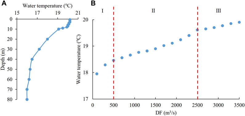
FIGURE 7. Optimization and scheduling results of discharge water temperature on 27 September 2022. (A) Observed vertical water temperature in front of the dam on 27 September 2022. (B) The optimized scheduling results of discharge water temperature based on discharge flow regulation are divided into three zones: I (the discharge flow range is 0–500 m³/s), II (the discharge flow range is 500–2,500 m³/s), and III (the discharge flow range is 2,500–3,500 m³/s).

3.5 Future perspective

The Dadu River is located in the upper reaches of the Yangtze River and is a typical representation of China’s hydropower development (Duan et al., 2020). At present, a 28 level hydropower plan has been developed for the Dadu River Basin. With the operation of cascade reservoirs, its cumulative impact on the water ecology is difficult to estimate. In this study, we only conducted ML modeling of the DWT of the PBGR, a reservoir in the Dadu River. This model can provide decision-making support for the management of the DWT of the PBGR in terms of reservoir operation. In the future, a prediction model for the water temperature of cascade reservoirs in the Dadu River Basin should be established based on the model constructed in this study. In addition, this study only conducted a simple analysis of regulating the DF to regulate the DWT. In fact, reservoir scheduling needs to consider various factors, such as power generation, water quality, water quantity, etc. In the future, based on the DWT model constructed in this study, coupled with the models of other considering factors, an optimized operation model can be constructed to determine the optimal operation mode of the reservoir.

4 Conclusion

The DWT is the boundary condition of downstream river water temperature and has a significant impact on the ecological health of downstream water. Accurately predicting the water temperature of reservoir discharge is helpful for the ecological protection of downstream river water. We constructed a refined artificial intelligence prediction model for DWT according to high-frequency monitoring data of the PBGR. Based on the influence mechanism of the DWT, the RVWT, WL, and DF were chosen as input indicators. We compared the performance of six models: SVR, KNN, MLPNN, LR, RFR, and GBRT. The SVR model with RBF had the best performance among these models. The genetic algorithm was used for parameter optimization, and on the validation set, the R² of the SVR model was 0.979. The performance of the SVR model based on optimal parameters on the test set was as follows: RMSE = 0.490°C, MAE = 0.272°C, and NSE = 0.976. A 1–24 h early warning model was constructed based on the SVR model, which had slightly worse performance than that of the non-early warning model. However, the performance of this model was still within an acceptable range. Finally, based on the SVR model, we optimized the scheduling of DWT and found that the constructed model has high generalization ability, effectively identifying the nonlinear relationship between DWT and DF. The constructed model can provide short-term forecasting and decision-making references for reservoir management decision-makers.

Data availability statement

The data analyzed in this study is subject to the following licenses/restrictions: Confidentiality Agreement with Reservoir Management Company. Requests to access these datasets should be directed to GC, chen_gang_ddh@163.com.

Author contributions

XH: Conceptualization, Data curation, Formal Analysis, Investigation, Methodology, Writing–original draft, Writing–review and editing. GC: Funding acquisition, Project administration, Supervision, Writing–review and editing.

Funding

The author(s) declare financial support was received for the research, authorship, and/or publication of this article. This work was supported by the Key R&D Projects of Sichuan Science and Technology Plan (2022YFG0120).

Conflict of interest

Authors XH and GC were employed by Da Du River Hydropower Development Co., Ltd.

Publisher’s note

All claims expressed in this article are solely those of the authors and do not necessarily represent those of their affiliated organizations, or those of the publisher, the editors and the reviewers. Any product that may be evaluated in this article, or claim that may be made by its manufacturer, is not guaranteed or endorsed by the publisher.

References

Alavian, V., Jirka, G. H., Denton, R. A., Johnson, M. C., and Stefan, H. G. (1992). Density currents entering lakes and reservoirs. J. Hydraulic Eng. 118, 1464–1489. doi:10.1061/(asce)0733-9429(1992)118:11(1464)

CrossRef Full Text | Google Scholar

Alibrahim, H., and Ludwig, S. A. (2021). “Hyperparameter optimization: comparing genetic algorithm against grid search and bayesian optimization,” in 2021 IEEE Congress on Evolutionary Computation (CEC), Kraków, Poland, 28 June 2021 - 01 July 2021 (IEEE), 1551–1559.

CrossRef Full Text | Google Scholar

Alwadai, N., Khan, S.U.-D., Elqahtani, Z. M., and Khan, S.U.-D. (2022). Machine learning assisted prediction of power conversion efficiency of all-small molecule organic solar cells: a data visualization and statistical analysis. Molecules 27, 5905. doi:10.3390/molecules27185905

PubMed Abstract | CrossRef Full Text | Google Scholar

Bangfu, C., Dongsheng, W., Di, Z., and Qidong, P. (2022). Conservation of aquatic ecosystems and fish species during hydropower development in the river basin: case study for the Dadu River Basin. Water Resour. Hydropower Eng. 53, 347–357. doi:10.13928/j.cnki.wrahe.2022.S1.057

CrossRef Full Text | Google Scholar

Barbarossa, V., Bosmans, J., Wanders, N., King, H., Bierkens, M. F. P., Huijbregts, M. A. J., et al. (2021). Threats of global warming to the world’s freshwater fishes. Nat. Commun. 12, 1701. doi:10.1038/s41467-021-21655-w

PubMed Abstract | CrossRef Full Text | Google Scholar

Booker, D. J., and Whitehead, A. L. (2022). River water temperatures are higher during lower flows after accounting for meteorological variability. River Res. Appl. 38, 3–22. doi:10.1002/rra.3870

CrossRef Full Text | Google Scholar

Croghan, D., Van Loon, A. F., Sadler, J. P., Bradley, C., and Hannah, D. M. (2019). Prediction of river temperature surges is dependent on precipitation method. Hydrol. Process. 33, 144–159. doi:10.1002/hyp.13317

CrossRef Full Text | Google Scholar

Duan, B., Chen, G., Tang, M., and Yan, Q. (2020). Early demonstration and research on the key technical issues of large-basin hydropower development under the concept of harmony. Clean. Energy 4, 67–74. doi:10.1093/ce/zkz016

CrossRef Full Text | Google Scholar

Gao, X., Li, G., and Han, Y. (2014). Effect of flow rate of side-type orifice intake on withdrawn water temperature. Sci. World J. 2014, 1–7. doi:10.1155/2014/979140

PubMed Abstract | CrossRef Full Text | Google Scholar

Ge, Z., Geng, Y., Wei, W., Jiang, M., Chen, B., and Li, J. (2023). Embodied carbon emissions induced by the construction of hydropower infrastructure in China. Energy Policy 173, 113404. doi:10.1016/j.enpol.2022.113404

CrossRef Full Text | Google Scholar

Gray, R., Jones, H. A., Hitchcock, J. N., Hardwick, L., Pepper, D., Lugg, A., et al. (2019). Mitigation of cold-water thermal pollution downstream of a large dam with the use of a novel thermal curtain. River Res. Appl. 35, 855–866. doi:10.1002/rra.3453

CrossRef Full Text | Google Scholar

Guo, G. D., Wang, H., Bell, D., Bi, Y. X., and Greer, K. (2006). Using kNN model for automatic text categorization. Soft Comput. 10, 423–430. doi:10.1007/s00500-005-0503-y

CrossRef Full Text | Google Scholar

He, W., Lian, J., Du, H., and Ma, C. (2018). Source tracking and temperature prediction of discharged water in a deep reservoir based on a 3-D hydro-thermal-tracer model. J. Hydro-Environment Res. 20, 9–21. doi:10.1016/j.jher.2018.04.002

CrossRef Full Text | Google Scholar

Hebert, C., Caissie, D., Satish, M. G., and El-Jabi, N. (2014). Modeling of hourly river water temperatures using artificial neural networks. Water Qual. Res. J. 49, 144–162. doi:10.2166/wqrjc.2014.007

CrossRef Full Text | Google Scholar

Jiang, D., Xu, Y., Lu, Y., Gao, J., and Wang, K. (2022). Forecasting water temperature in cascade reservoir operation-influenced river with machine learning models. Water 14, 2146. doi:10.3390/w14142146

CrossRef Full Text | Google Scholar

Labaj, A. L., Michelutti, N., and Smol, J. P. (2016). Changes in cladoceran assemblages from tropical high mountain lakes during periods of recent climate change. J. Plankton Res. 39, 211–219. doi:10.1093/plankt/fbw092

CrossRef Full Text | Google Scholar

Larabi, S., Schnorbus, M. A., and Zwiers, F. (2022). A coupled streamflow and water temperature (VIC-RBM-CE-QUAL-W2) model for the Nechako Reservoir. J. Hydrology-Regional Stud. 44, 101237. doi:10.1016/j.ejrh.2022.101237

CrossRef Full Text | Google Scholar

Li, S., and Zhang, Q. (2014). Carbon emission from global hydroelectric reservoirs revisited. Environ. Sci. Pollut. Res. 21, 13636–13641. doi:10.1007/s11356-014-3165-4

PubMed Abstract | CrossRef Full Text | Google Scholar

Liashchynskyi, P., and Liashchynskyi, P. (2019). Grid search, random search, genetic algorithm: a big comparison for NAS. Arxiv [Preprint]. Available at: https://arxiv.org/abs/1912.06059.

Google Scholar

Liu, C., Lian, J., and Wang, H. (2022). Experimental analysis of temperature-control curtain regulating outflow temperature in a thermal-stratified reservoir. Int. J. Environ. Res. Public Health 19, 9472. doi:10.3390/ijerph19159472

PubMed Abstract | CrossRef Full Text | Google Scholar

Lu, H., and Ma, X. (2020). Hybrid decision tree-based machine learning models for short-term water quality prediction. Chemosphere 249, 126169. doi:10.1016/j.chemosphere.2020.126169

PubMed Abstract | CrossRef Full Text | Google Scholar

Lu, Y., Tuo, Y., Xia, H., Zhang, L., Chen, M., and Li, J. (2023). Prediction model of the outflow temperature from stratified reservoir regulated by stratified water intake facility based on machine learning algorithm. Ecol. Indic. 154, 110560. doi:10.1016/j.ecolind.2023.110560

CrossRef Full Text | Google Scholar

Meng, Y., Zhang, X., and Zhang, X. (2023). Identification modeling of ship nonlinear motion based on nonlinear innovation. Ocean. Eng. 268, 113471. doi:10.1016/j.oceaneng.2022.113471

CrossRef Full Text | Google Scholar

Quan, Q., Zou, H., Huang, X., and Lei, J. (2022). Research on water temperature prediction based on improved support vector regression. Neural Comput. Appl. 34, 8501–8510. doi:10.1007/s00521-020-04836-4

CrossRef Full Text | Google Scholar

Ren, L., Wu, W., Song, C., Zhou, X., and Cheng, W. (2019). Characteristics of reservoir water temperatures in high and cold areas of the Upper Yellow River. Environ. Earth Sci. 78, 160. doi:10.1007/s12665-019-8144-0

CrossRef Full Text | Google Scholar

Shaoxiong, Z., Wenzhi, C., Liting, Z., and Xiang, G. (2019). Numerical simulation on temperature of water released from multi-level intake of reservior. IOP Conf. Ser. Earth Environ. Sci. 304, 022018. doi:10.1088/1755-1315/304/2/022018

CrossRef Full Text | Google Scholar

Sivri, N., Ozcan, H. K., Ucan, O. N., and Akincilar, O. (2009). Estimation of stream temperature in degirmendere river (trabzon-Turkey) using artificial neural network model. Turk J. Fish. Aquat. Sci. 9, 145–150. doi:10.4194/trjfas.2009.0204

CrossRef Full Text | Google Scholar

Soleimani, S., Bozorg-Haddad, O., Saadatpour, M., and Loaiciga, H. A. (2016). Optimal selective withdrawal rules using a coupled data mining model and genetic algorithm. J. Water Resour. Plan. Manag. 142, 717. doi:10.1061/(asce)wr.1943-5452.0000717

CrossRef Full Text | Google Scholar

Song, Q., Sun, B., Gao, X., and Liu, Y. (2020). Laboratory investigation on the influence of factors on the outflow temperature from stratified reservoir regulated by temperature control curtain. Environ. Sci. Pollut. Res. 27, 33052–33064. doi:10.1007/s11356-020-09507-4

PubMed Abstract | CrossRef Full Text | Google Scholar

Song, Z., Song, J., and Yue, B. (2008). Population genetic diversity of Prenant’s schizothoracin, Schizothorax prenanti, inferred from the mitochondrial DNA control region. Environ. Biol. Fishes 81, 247–252. doi:10.1007/s10641-007-9197-6

CrossRef Full Text | Google Scholar

Velasco, L. C. P., Serquina, R. P., Abdul Zamad, M. S. A., Juanico, B. F., and Lomocso, J. C. (2019). Performance analysis of multilayer perceptron neural network models in week-ahead rainfall forecasting. Int. J. Adv. Comput. Sci. Appl. 10, 578–588. doi:10.14569/ijacsa.2019.0100374

CrossRef Full Text | Google Scholar

Wang, H., Deng, Y., Yan, Z., Yang, Y., and Tuo, Y. (2023). Thermal response of a deep monomictic reservoir to selective withdrawal of the upstream reservoir. Ecol. Eng. 187, 106864. doi:10.1016/j.ecoleng.2022.106864

CrossRef Full Text | Google Scholar

Wang, H., Deng, Y., Yang, Y., Chen, M., Wang, X., and Tuo, Y. (2024). Future projections of thermal regimes and mixing characteristics in a monomictic reservoir under climate change. Sci. Total Environ. 906, 167527. doi:10.1016/j.scitotenv.2023.167527

PubMed Abstract | CrossRef Full Text | Google Scholar

Wang, L., Xu, B., Zhang, C., Fu, G., Chen, X., Zheng, Y., et al. (2022a). Surface water temperature prediction in large-deep reservoirs using a long short-term memory model. Ecol. Indic. 134, 108491. doi:10.1016/j.ecolind.2021.108491

CrossRef Full Text | Google Scholar

Wang, Z., Feng, J., Liang, M., Wu, Z., Li, R., Chen, Z., et al. (2022b). Prediction model and application of machine learning for supersaturated total dissolved gas generation in high dam discharge. Water Res. 220, 118682. doi:10.1016/j.watres.2022.118682

PubMed Abstract | CrossRef Full Text | Google Scholar

Weber, M., Rinke, K., Hipsey, M., and Boehrer, B. (2018). Optimizing withdrawal from drinking water reservoirs to reduce downstream temperature pollution and reservoir hypoxia. J. Environ. Manag. 197, 96–105. doi:10.1016/j.jenvman.2017.03.020

PubMed Abstract | CrossRef Full Text | Google Scholar

Xu, N., Wang, Z., Dai, Y., Li, Q., Zhu, W., Wang, R., et al. (2023). Prediction of higher heating value of coal based on gradient boosting regression tree model. Int. J. Coal Geol. 274, 104293. doi:10.1016/j.coal.2023.104293

CrossRef Full Text | Google Scholar

Yang, X., Tuo, Y., Yang, Y., Wang, X., Deng, Y., and Wang, H. (2021). Study on the effect of front retaining walls on the thermal structure and outflow temperature of reservoirs. PLoS ONE 16, e0260779. doi:10.1371/journal.pone.0260779

PubMed Abstract | CrossRef Full Text | Google Scholar

Yang, Y., Deng, Y., Tuo, Y., Li, J., He, T., and Chen, M. (2020). Study of the thermal regime of a reservoir on the Qinghai-Tibetan Plateau, China. PLoS ONE 15, e0243198. doi:10.1371/journal.pone.0243198

PubMed Abstract | CrossRef Full Text | Google Scholar

Yong-Bo, C., Yun, D., and Rui-Feng, L. (2010). “IMPACT OF STOPLOG INTAKE WORKS ON RESERVOIR DISCHARGED WATER TEMPERATURE,” in Resources & environment in the Yangtze basin (Beijing P.R.China: National Science Library).

Google Scholar

Yoon, H. (2021). Finding unexpected test accuracy by cross validation in machine learning. Int. J. Comput. Sci. Netw. Secur. 21, 549–555. doi:10.22937/IJCSNS.2021.21.12.76

CrossRef Full Text | Google Scholar

Zhang, D., Wang, D., Peng, Q., Lin, J., Jin, T., Yang, T., et al. (2022). Prediction of the outflow temperature of large-scale hydropower using theory-guided machine learning surrogate models of a high-fidelity hydrodynamics model. J. Hydrology 606, 127427. doi:10.1016/j.jhydrol.2022.127427

CrossRef Full Text | Google Scholar

Zhang, Y., Wu, Z., Liu, M., He, J., Shi, K., Zhou, Y., et al. (2015). Dissolved oxygen stratification and response to thermal structure and long-term climate change in a large and deep subtropical reservoir (Lake Qiandaohu, China). Water Res. 75, 249–258. doi:10.1016/j.watres.2015.02.052

PubMed Abstract | CrossRef Full Text | Google Scholar

Zhang, Z., and Xu, J. (2014). Applying rough random MODM model to resource-constrained project scheduling problem: a case study of Pubugou Hydropower Project in China. Ksce J. Civ. Eng. 18 (5), 1279–1291. doi:10.1007/s12205-014-0426-1

CrossRef Full Text | Google Scholar

Zhou, C., Tuo, Y., Li, K., Deng, Y., and Liang, R. (2016). Investigation into the influence of water temperature of Pubugou reservoir. J. Sichuan Univ. Eng. Sci. Ed. 48, 27–33. doi:10.15961/j.jsuese.2016.s2.005

CrossRef Full Text | Google Scholar

Zhu, S., Bonacci, O., Oskoru, D., Hadzima-Nyarko, M., and Wu, S. (2019). Long term variations of river temperature and the influence of air temperature and river discharge: case study of Kupa River watershed in Croatia. J. Hydrology Hydromechanics 67, 305–313. doi:10.2478/johh-2019-0019

CrossRef Full Text | Google Scholar

Zhu, S., and Piotrowski, A. P. (2020). River/stream water temperature forecasting using artificial intelligence models: a systematic review. Acta Geophys. 68, 1433–1442. doi:10.1007/s11600-020-00480-7

CrossRef Full Text | Google Scholar