Predicting groundwater level using traditional and deep machine learning algorithms

1 Introduction

The groundwater level (GWL) is of critical importance, especially in arid and semi-arid countries (Alfarrah and Walraevens, 2018; Bovolo et al., 2009; Priyan, 2021). In many areas, the overexploitation of GWL has led to irreparable damage to the groundwater sources (Alfarrah and Walraevens, 2018; Bovolo et al., 2009; Priyan, 2021). Predicting GWL is a key challenge in hydrogeological investigations, effective aquifer management, and assessment of subterranean water volume (Sun et al., 2022; Barzegar et al., 2017). Hydrogeological studies have been conducted to estimate the potential of underground water, predict changes in the GWL, and examine the current state of underground water resources (Hay and Mimura, 2005; Russo and Taddia, 2009). Empirical time series models have been extensively used to predict GWL levels (Eriksson, 1970). The ability of empirical or numerical models such as finite element groundwater flow system (FEFLOW)¹ (Ma et al., 2022), modular finite-difference flow model (MODFLOW)² (Hughes et al., 2022), and HydroGeoSphere³ (Kang et al., 2017) to estimate the GWL has made these models helpful in predicting the GWL (Trefry and Muffels, 2007; Wang et al., 2008; Brunner and Simmons, 2012).

1.1 Problem statement

The prediction of GWL is crucial for sustainable water resource management, as accurate forecasts contribute to understanding the availability and distribution of groundwater, essential for purposes such as agriculture, drinking water supply, and ecosystem maintenance (Singh et al., 2021a; Pragnaditya et al., 2021; Khan et al., 2023). Machine learning (ML) techniques offer the potential to analyze large and complex datasets, identify patterns, and make predictions that inform decision-making in water resource management (Singh, 2015; Singh et al., 2021b; Pham et al., 2022; Ghobadi and Kang, 2023; Singh et al., 2024). By applying ML to predict GWL, we can enhance our ability to monitor and manage water resources effectively, ensuring their sustainable use over time (Tao et al., 2022a; Pham et al., 2022). However, in Izeh City, Khuzestan province of Iran, certain challenges, such as low rainfall, increasing temperature, consecutive droughts, and overexploitation of GWL for agricultural purposes, create gaps in the prediction of GWL for this region. The absence of accurate predictive models tailored to Izeh City’s unique context poses a significant obstacle to achieving reliable predictions. Addressing these challenges is crucial for developing robust ML models that accurately forecast GWL in the region, thereby facilitating more effective water resource management strategies.

1.2 Literature review

Using the mathematical model of the aquifer is one of the best methods for managing and controlling the drop in water levels (Rajaee et al., 2019). In GWL mathematical models, differential equations are utilized to simulate GWL flow (Rajaee et al., 2019). Since the dynamic behavior of a hydrological system changes with the passage of time, the indicated models do not have adequate ability to predict the characteristics of water resources and are not suitable models (Rathinasamy et al., 2014). Physical models generally excel at capturing and delineating the relationships between variables, as they are built upon established scientific principles and laws. These models are grounded in a fundamental understanding of the underlying processes and mechanisms governing the system under consideration. This allows physical models to provide valuable insights into the behavior and interactions of various components within the system. Since the relationships between the variables affecting the GWL are complex and non-linear, physical models in practice require a lot of data to simulate the fluctuations of the GWL (Nayak et al., 2006; Khan and Valeo, 2016). Deep learning models, while powerful in terms of prediction performance, are often considered black-box models with limited interpretability, making it challenging to understand the exact relationships between variables. Based on artificial neural network (ANN), these models have shown remarkable success in various fields, such as image recognition, natural language processing, and gameplay (Nadiri et al., 2013).

Researchers have developed innovative approaches to predict the water level in aquifers in light of the numerous issues with artificial models for modeling aquifers (Tao et al., 2022b). Artificial intelligence (AI) models have been applied in a number of areas recently, including hydrogeological and underground water research (Nadiri et al., 2014). AI algorithms can use sparse, brief data to mimic irregular and non-linear time series with high accuracy. Due to their accuracy and usefulness, these models have been employed in recent years to anticipate the GWL (Franses and Van Dijk, 2000). Gong et al. (2015) tested the validity of three nonlinear time-series intelligence models, namely ANN, support vector machine (SVM), and adaptive neuro-fuzzy inference system (ANFIS), for the prediction of GWL considering surface water-groundwater interaction. The models were applied to two wells near Lake Okeechobee in Florida, United States, using a 10-year dataset of hydrological parameters. Evaluation measures showed that the ANFIS and SVM models provided more accurate predictions than the ANN model. Taking into account the surface water-groundwater interaction improved the prediction accuracy, particularly in areas close to the surface water, such as the lake area (Gong et al., 2016). Wen et al. (2017) introduced the wavelet analysis–artificial neural network (WA-ANN) model to predict the GWL in China for the next 1, 2, and 3 months. GWL, climate data, and water level were taken into consideration as input data in this study. They concluded that the suggested model is most accurate when the previous GWL is used as input data. In conclusion, it can be claimed that the WA-ANN model is a reliable and effective tool for estimating GWL (Wen et al., 2017). Kaya et al. (2018) used 196 data points from 2000 to 2015 to predict the GWL in the Turkish province of Reyhanli. They applied ANN and M5tree (M5T) model approaches in their investigation. They claimed that the methodologies suggested in this study are remarkably accurate for estimating the GWL and that the approaches presented in this study perform effectively (Kaya et al., 2018). Zhang et al. (2018) developed a Long short-term memory (LSTM) time series model to predict water table depth in agricultural areas with complex hydrogeological characteristics. Their proposed model outperformed the traditional feed-forward neural network (FFNN) in GWL prediction, achieving higher R² scores (0.789–0.952). The dropout method effectively prevented overfitting, and the model’s architecture demonstrated a strong learning ability on time series data. The study suggests that the LSTM-based model can be a valuable alternative for the prediction of GWL, particularly in data-scarce areas (Zhang et al., 2018). Kombo et al. (2020) introduced the K-Nearest Neighbour-random forest (KNN-RF) model along with ANN, KNN, SVM, and RF models to predict changes in the GWL of an aquifer in eastern Rwanda. The KNN-RF model is more accurate than other models, as they determined from their research. They asserted that planning and managing GWL resources can benefit from the KNN-RF approach (Kombo et al., 2020). Kumar et al. (2020) predicted GWL using a DL model alongside extreme learning machine (ELM) and Gaussian process regression (GPR) models, in the Konan basin, Japan. They assessed the DL model’s accuracy, which showed excellent agreement during validation (RMSE = 0.08, r = 0.95, NSE = 0.87). Re-validation at different stations demonstrated its robustness and generalization capabilities, making it a reliable tool for predicting GWL and optimizing resource allocation in groundwater systems (Kumar et al., 2020). Sharafati et al. (2020) employed gradient boosting regression (GBR) to predict monthly GWL in the Rafsanjan aquifer, Iran, using various input variables, including satellite data and pumping rates. They used the gamma test (GT) for feature selection and assessed performance using error metrics. The GBR yielded high predictive accuracy, especially with the gravity recovery and climate experiment (GRACE) dataset (Sharafati et al., 2020). Correlation analysis showed coefficient of determination values ranging from 0.66 to 0.94 for different lead times, with better accuracy in regions with higher water depth and pumping rates. The study offers valuable insights for water resource planning based on accurate modeling (Sharafati et al., 2020). Banadkooki et al. (2020) aimed to predict GWL using precipitation and temperature data with various temporal delays. They employed the radial basis function–whale algorithm (RBF-WA), multilayer perception (MLP–WA), and genetic programming (GP) to build hybrid ANN models. Results showed that the MLP–WA model outperformed others when using temperature data with delays of 3, 6, and 9 months. Combining precipitation and temperature data with these delays yielded the best results (Banadkooki et al., 2020).

Osman et al. (2021) used three Xgboost models, an ANN, and vector regression to predict the GWL in Selangor, Malaysia. This study used 11 months from October 2017 to July 2018 to collect data for the models, including rainfall, temperature, previous day’s water level, and evaporation. The study’s conclusions showed that the Xgboost model produces more accurate prediction results (Osman et al., 2021). Malakar et al. (2021) predicted future GWL trends in India using GRACE-derived GWS, WaterGap model-based GWR, and GWW. Their LSTM model outperformed FNN and RNN, showing >84% of wells with r > 0.6 and RMSE <0.7. They anticipate declining GWL trends in northwest, north-central, and south India, which could impact water supply and crop production for 1.3 billion people (Malakar et al., 2021). Afan et al. (2021) employed deep learning (DL) and ensemble deep learning (EDL) techniques to predict GWL in Malaysia. Their results revealed that EDL outperformed DL in estimating GWL, except for the Paya Indah Wetland. Additionally, EDL demonstrated superior performance in predicting daily GWL across all stations, reducing errors and providing precise results within a shorter time lag. Overall, they revealed that the EDL model has the potential to contribute to the sustainable management of GWL in Malaysia (Afan et al., 2021). Khan et al. (2023) reviewed GWL prediction models comprehensively. They examined 109 research articles and concluded that ML and deep learning approaches are efficient for modeling GWL. They also suggested future research directions to enhance prediction accuracy and understanding in this field (Khan et al., 2023). Dehghani and Torabi Poudeh, (2022) predicted GWL in southwest Iran by employing several meta-heuristic algorithms, including Feed-forward neural network (FNN) and automated item generation (AIG) models. Utilizing data on monthly rainfall, temperature, and water table height from the Lorestan Regional Water Corporation spanning 2008 to 2018, their study demonstrated the superior accuracy of the ANN-AIG hybrid model compared to other methods (Dehghani and Torabi Poudeh, 2022). Mohammed et al. (2023) combined a numerical model called GMS with methods like GA-ANN, GA-ICA, extreme learning machine (ELM), and ORELM in order to predict the GWL using piezometric data and rainfall information. The results of this investigation showed that, compared to other methods, the ORELM method accurately predicts the level of GWL (Mohammed et al., 2023). Table 1 shows the research work for the literature reviews used to predict GWL.

TABLE 1

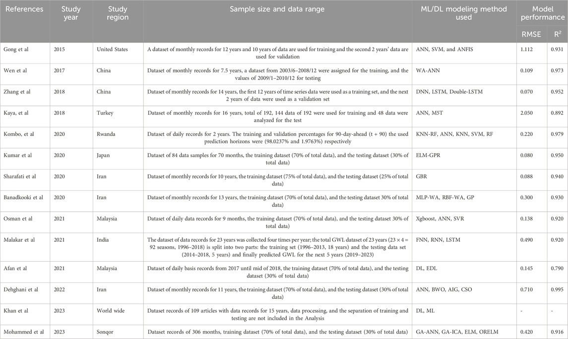
TABLE 1. List of the previous work on the prediction of the GWL based on DML.

So far, no systematic study has been conducted to estimate the GWL in Izeh City, which is located in the Khuzestan province of Iran. Given that the region’s primary occupation is agriculture and the prevalent use of GWL for domestic, agricultural, and industrial purposes, accurate GWL prediction can significantly impact water supply and crop production in this area.

2 Methodology

The diagram depicted in Figure 1 illustrates the prediction procedure for GWL employing both traditional and deep ML algorithms, including DT, RF, SVM, CNN, GAN, and RNN. The initial step of executing this methodology involves the collection of data from Iran’s study area. Subsequently, the dataset undergoes sorting and preprocessing stages, which encompass the removal of outliers and duplicate data points. Following this, the data points are normalized using Eq. (1).

${\omega }_i^l=\left(\frac{{\omega }_i^l-{\omega \mathit{min}}^l}{{\omega \mathit{max}}^l-{\omega \mathit{min}}^l}\right)\ast 2-1(1)$

FIGURE 1

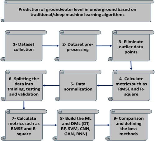
FIGURE 1. Illustration of a flowchart for prediction of GWL based on traditional and deep ML (DT, RF, SVM, CNN, GAN, and RNN).

Finally, the dataset is randomly partitioned into training, testing, and validation sets. To compare traditional and deep ML, various metrics, such as RMSE and R-Square, are computed for each algorithm. Sophistic ML models like CNN, GAN, and RNN are developed using preprocessed data. Ultimately, the models’ performances are juxtaposed, leading to the selection of CNN as the optimal approach for predicting GWL.

2.1 Traditional machine learning

2.1.1 Decision tree (DT)

The DT is a widely used supervised ML algorithm that is particularly valuable for classification and prediction tasks by dividing data into sub-trees and branching out further (Kotsiantis, 2013). In this algorithm, the input variables (R, P, and E) are considered trees, and the control parameters related to the RF algorithm are considered nodes between the trees. Finally, the final decision is known as the GWL prediction. This study employed a regression decision tree model with specified parameters. The maximum depth of the tree was set to 100, indicating the maximum number of levels in the tree structure. The criterion for measuring the quality of a split was chosen as “Gini,” which typically assesses impurity for classification tasks, although it is worth noting that for regression tasks, other criteria like “mse” (Mean Squared Error) might be more common. The splitter strategy was set to “best,” meaning the algorithm considers all possible splits and selects the one that optimally reduces impurity or minimizes the mean squared error.

2.1.2 Random forest (RF)

The RF algorithm amalgamates the predictions stemming from all constituent trees within the forest, averaging them to yield a prediction that is not only more robust but also more accurate (Gomes et al., 2017). This ensemble approach effectively counteracts the influence of individual trees that might have generated erroneous predictions or excessively adhered to the training data’s idiosyncrasies. In this algorithm (RF) context, the input and output variables (R, P, E, and GWL) are metaphorically conceptualized as trees. The aggregate decisions and the ultimate amalgamated tree are denoted as the GWL outcomes upon culmination. This study employed a regression random forest model with specific parameter settings. The maximum depth of the trees in the forest was set to 100, indicating the maximum number of levels in each decision tree. The random state was fixed at 0, ensuring reproducibility by keeping the randomness constant. The number of decision trees in the forest was set to 0, which typically means an unrestricted growth of trees until the specified maximum depth is reached. The objective function used for training the model was the Mean Squared Error (MSE), a measure that quantifies the average squared difference between the predicted and actual values, guiding the optimization process toward minimizing prediction errors.

2.1.3 Support vector machines (SVM)

The versatility of SVM is evident in its utilization for both classification and regression tasks, mirroring the functionalities of DT and RF algorithms (Wang et al., 2022). The algorithm diligently endeavors to expand these margins to their fullest potential, effectively delving into the essence of generalized error learning theory and striving to minimize errors to the greatest extent possible (Kecman, 2001). This endeavor aligns with SVM’s overarching objective of achieving optimal separation between distinct classes or the prediction of accurate numerical values in regression scenarios (Ozer et al., 2020). In this algorithm, the input variables (R, P, and E) are the objective parameters discussed in this article, while the output variable (GWL) is the predictive parameter. In this study, a prediction model was developed with specific hyperparameters: a batch size of 100, determining the number of training samples processed in a single iteration; a regularization parameter (C), which helps control overfitting by penalizing significant coefficients in the model, set to 0.1; and the utilization of a polynomial kernel.

2.2 Deep machine learning

2.2.1 Recurrent neural network (RNN)

An RNN is a specialized neural network for handling sequential and time-series data, particularly suited for prediction GWL based on input parameters P, R, and E (Panahi et al., 2020). Unlike multilayer perceptron (MLP) and CNN architectures, RNNs emphasize time considerations. While feed-forward networks like CNNs are common, RNNs incorporate a feedback loop, enabling them to retain prior inputs and process input sequences, preserving information across moments (Kanjo et al., 2019; Garbin et al., 2020). This characteristic ensures historical data’s retention within the network. Figure 2A presents an RNN cell example (Han et al., 2021).

FIGURE 2

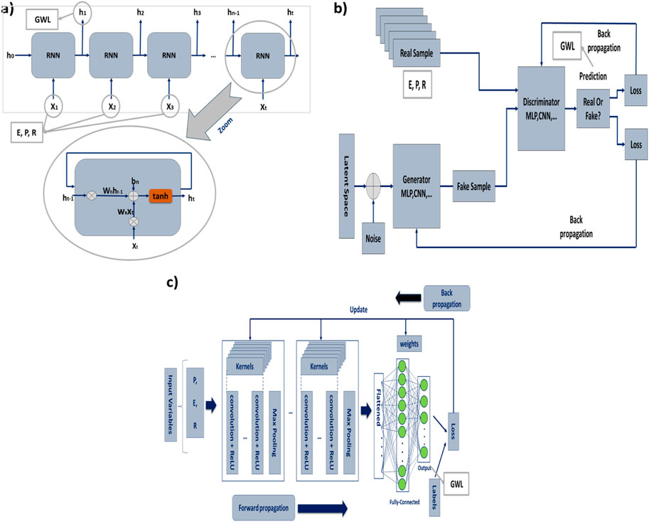
FIGURE 2. Illustration of the (A) chain of RNN network, (B) GAN network, (C) CNN algorithm for prediction of GWL.

An RNN consists of a hidden state memory input (‘h’) and a primary input ‘x’ (R, E, and P) (Ming et al., 2017). Processing occurs through layers ‘wh’ and ‘wx’ for ‘h' and ‘x’, respectively. ‘ht-1’ and ‘xt’ is multiplied by ‘wh’ and ‘wx’ weight matrices (Mirsalari et al., 2020) summed as per Eq. (2), and activated by functions like tanh, sigmoid, relu, etc. (Giordano et al., 2019) to yield ‘ht.’ See Figure 2A for the RNN architecture.

$h_t=\mathrm{f}\left(w_h{h}_{t-1}+w_x{x}_t+b_h\right)(2)$

The output above corresponds to the next hidden state (h_t) and the output of the RNN at time t. In Figure 2A X (1) serves as the input sequence; h (0) and X (1) combine for the subsequent stage. Outputs h (1) and X (2) in the following stage form input. During training, previous inputs are remembered (Shi et al., 2017). Unfolding the RNN over time creates a network chain. Hyperparameters are detailed in Table 2. In the realm of predicting GWL using an RNN algorithm, controlling chaos is important for stability. Adjusting the time constant for model units aids in capturing the system’s dynamics while optimizing the learning rate to fine-tune the model’s responsiveness. The time constant of filtered white noise inputs and the weight assigned to white noise inputs influence noise incorporation, demanding careful calibration. Iterating the training process and modifying the data time step size ensures model accuracy with evolving data patterns. Furthermore, the RNN integration step size impacts temporal resolution, necessitating strategic adjustments to balance precision and computational efficiency in predicting GWL.

TABLE 2

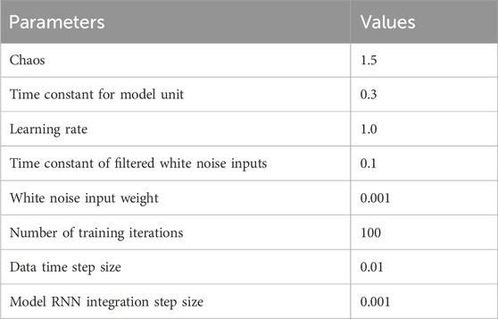
TABLE 2. The hyperparameters for RNN algorithm.

2.2.2 Generative adversarial networks (GAN)

The GANs, comprising a generator and a discriminator, identify data patterns autonomously, engaging in a competition to evolve the dataset (Shi et al., 2017). Figure 2B shows a GAN network.

The GANs consist of two neural networks: a generator G(x) and a discriminator D(x). The generator produces synthetic samples to increase the likelihood of fooling the discriminator (Dong and Lin, 2019). It takes noise vectors and generates fake data. Real and fake data are then fed to the discriminator, which categorizes them (Li et al., 2019). The model is trained by calculating the loss at the discriminator’s end and adjusting parameters via backpropagation (Alarsan and Younes, 2021). The GAN training process involves selecting real data (X), passing it through the generator and applying sigmoid activation, creating noise data (Z), generating samples (G(Z)), evaluating loss, backpropagating to update discriminator weights, using generator output to update its weights, and iterating until optimal weights are achieved for both networks.

The discriminator loss function assesses D’s prediction on real/fake data, calculated from errors made. Errors backpropagate to update parameters (Azari et al., 2022). It comprises terms for real (x) and fake (G(z)) inputs, with the real input loss term defined as expressed in Eq. (3). The second term is for fake input (G(z)) as expressed in Eq. (4).

$l_{d_1}=\mathit{log}\sigma \left(D\left(x\right)\right)(3)$

$l_{d_2}=\log (1-\sigma \left(D\left(G\left(z\right)\right)\right)(4)$

In the equation, σ is the sigmoid function with an output range of 0–1. An output near 1 implies accurate real data recognition by D, resulting in minimal loss (Szandała, 2021).

The two-loss terms are computed and summed for the overall discriminator network loss. The GAN hyperparameters, which are pivotal for performance, are detailed in Table 3. Due to GAN-type variance, tuning is essential. The generator time impacts training duration and data quality; the lower filter quantile prevents biased results, and the top filter quantile maintains alignment. The loss function improves GAN via data distinctions, and the maximum depth affects complexity and overfitting. The maximum bin and learning rate control convergence, ensuring reproducibility through a random state. Estimators boost diversity, batch size influences stability, and patience counters overfitting. Control parameters are fixed through careful calibration and iterative experimentation to optimize performance for the prediction of GWL.

TABLE 3

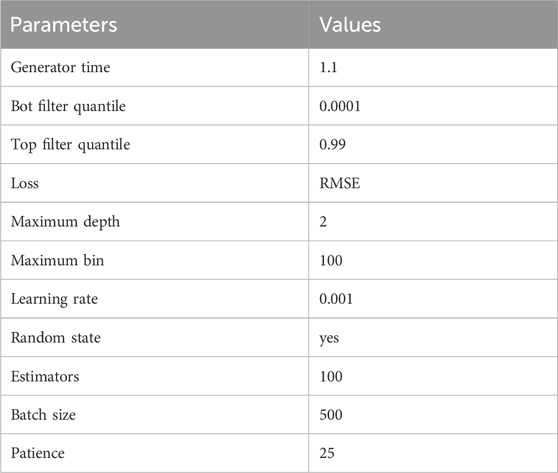
TABLE 3. The hyperparameters for the GAN algorithm.

2.2.3 Convolutional neural network (CNN)

The CNN emulates the visual cortex with neurons, weights, and biases. It comprises convolutional, pooling, and fully connected layers (Azizah et al., 2017). Notably, the convolutional layer employs operations, while the fully connected layer maps characteristics to output. The CNNs maintain input structure, highlighting data relationships (Yamashita et al., 2018). Training entails optimizing parameters via backpropagation and gradient descent. Figure 2C shows the structure of the CNN algorithm.

The main kernel of the CNN is the convolutional layer, which has assigned most of the computations to the CNN (Wang et al., 2017). Each convolutional layer in the CNN consists of a set of filters, and the output is created from the convolution between the filters and the input layer (O'Shea and Nash, 2015). The output of the convolutional layer is called a feature map.

In CNNs, the convolution operator slides a kernel over the input, multiplying its values with input values, creating a feature map (Wang et al., 2021). Kernel count and size dictate operation complexity, often 3 × 3, 5 × 5, or 7 × 7. The number determines the output feature map depth. Padding maintains input size. The CNN hyperparameters are in Table 4. Each control parameter serves a specific function in the CNN algorithm for predicting GWL. The input layer processes the initial data, the CONV layer extracts features through convolution, the POOL layer reduces spatial dimensions, and the Fully Connected layer combines features for classification. Softmax provides probability scores. Kernel size determines feature extraction scope, and Stride size controls filter movement. Fixing parameters involves tuning through iterative training and adjusting based on model performance and validation results.

TABLE 4

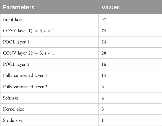
TABLE 4. The hyperparameters for the CNN algorithm.

2.3 Spearman’s and Pearson’s correlation and error metrics

One of the best methods for determining the relative importance of input-independent variables compared to output-dependent variables (GWL) is to use the Pearson’s coefficient (R) method. This coefficient expresses a correlation between −1 and +1. Based on this coefficient, a value of +1 has the most significant positive impact, and a value of −1 has the most significant absolute impact, while a zero value means there is no linear relationship between two variables. Also, this parameter shows that it has no effect. The Pearson’s correlation is shown in Eq. (5) (De Winter et al., 2016).

$Z=\frac{{\displaystyle \sum _{i=1}^n}\left(P_i-\overline{P}\right)\left(K_i-\overline{K}\right)}{\sqrt{{\displaystyle {\sum }_{i=1}^n}{\left(P_i-\overline{P}\right)}^2}\sqrt{{\displaystyle {\sum }_{i=1}^n}{\left(K_i-\overline{K}\right)}^2}}(5)$

Spearman’s coefficient (ρ) is one of the coefficients of the input data set compared to the output for the input variables compared to the output variables. Data can be ranked using this parameter. This equation is in the form of Eq. (6) (Alsaqr, 2021).

$\rho =\frac{{\displaystyle \sum _{i=1}^n}\left(P_i-\overline{P}\right)\left(K_i-\overline{K}\right)}{\sqrt{{\displaystyle {\sum }_{i=1}^n}{\left(P_i-\overline{P}\right)}^2{\displaystyle {\sum }_{i=1}^n}{\left(K_i-\overline{K}\right)}^2}}(6)$

In order to compare and measure the comparison, the equations and statistical errors reported in Equations (7–9) are used.

$\text{STD}=\sqrt{\frac{{\displaystyle {\sum }_{\mathrm{i}=1}^{\mathrm{n}}}{\left({\left(\frac{{\text{GWL}}_{\left(\text{Meas}.\right)}-{\text{GWL}}_{\left(\text{Pre}.\right)}}{{\text{GWL}}_{\left(\text{Meas}.\right)}}\mathrm{x}100\right)}_{\mathrm{i}}-\left(\frac{1}{\mathrm{n}}{\displaystyle \sum _{\mathrm{i}=1}^{\mathrm{n}}}\left({{\text{GWL}}_{\text{Meas}.}}_{\mathrm{i}}-{{\text{GWL}}_{\text{Pre}.}}_{\mathrm{i}}\right)\right)\right)}^2}{\mathrm{n}-1}}(7)$

$\text{RMSE}=\sqrt{\frac{1}{\mathrm{n}}{\displaystyle \sum _{\mathrm{i}=1}^{\mathrm{n}}}{\left({{\text{GWL}}_{\text{Meas}.}}_{\mathrm{i}}-{{\text{GWL}}_{\text{Pred}.}}_{\mathrm{i}}\right)}^2}(8)$

${\mathrm{R}}^2=1-\frac{{\displaystyle \sum _{\mathrm{i}=1}^{\mathrm{N}}}{\left({{\text{GWL}}_{\text{Meas}.}}_{\mathrm{i}}-{{\text{GWL}}_{\text{Pre}.}}_{\mathrm{i}}\right)}^2}{{\displaystyle \sum _{\mathrm{i}=1}^{\mathrm{N}}}{\left({{\text{GWL}}_{\text{Pre}.}}_{\mathrm{i}}-\frac{{\displaystyle {\sum }_{\mathrm{I}=1}^{\mathrm{n}}}{{\text{GWL}}_{\text{Meas}.}}_{\mathrm{i}}}{\mathrm{n}}\right)}^2}(9)$

3 Data gathering and data distribution

River water imports, precipitation, and the negative parameter of GWL withdrawal are among the positive parameters for GWL (Machiwal and Singh, 2015; Zhang et al., 2019). To predict this essential and vital parameter for human society, 2136-point data collected from 2018 to 2022 employing various methods, such as a water level sensor for groundwater level, a flow meter for groundwater extraction rate, a rain gauge for rainfall rate, and a stream gauge for river flow rate with 3 km distance, was gathered from Izeh City in the Khuzestan province of Iran for this article. BothIzeh City’s hydrology influences hydrology in Izeh City is influenced by human activities and seasonal changes (Kalantari et al., 2009; Hoseini, 2022). Human activities such as agriculture and industrialization significantly impact the region’s hydrological system (Nassery et al., 2009; Rashidi and Hosseinzadeh, 2019). Agricultural practices, particularly irrigation, heavily rely on E, which can lower the water level and alter the natural balance (Jafari et al., 2015; Neissi et al., 2020). Industrial activities and urbanization contribute to changes in surface runoff patterns and can introduce pollutants into water sources (Rashidi and Hosseinzadeh, 2019; Ziyari and Latifi, 2022). Additionally, seasonal variations play a crucial role in the hydrological cycle of Izeh City (Bakhtiari et al., 2021). During the rainy season, increased precipitation and runoff lead to rising GWL, while dry seasons result in decreased groundwater recharge due to higher evaporation rates (Kalantari et al., 2009). Understanding the intricate relationship between human activities, seasonal changes, and hydrology is vital for sustainable water resource management in Iran’s Izeh City of Khuzestan province (e.g., Nassery et al., 2009; Mahdavi et al., 2021).

In order to build a hybrid model of AI, 70% of the data is used for training, 15% for testing, and 15% for validation. The use of data to build the model is random. The statistical information related to the data used in this article is reported in Table 5. Based on this table, the range and values of statistical parameters are reported.

TABLE 5

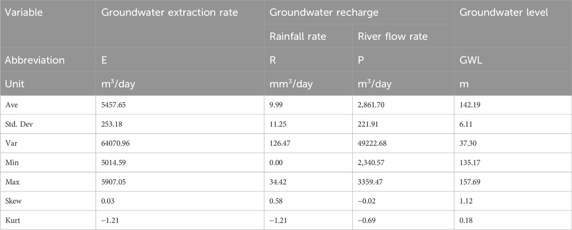
TABLE 5. Report of input/output variables in order to predict GWL for the data related to Izeh City of Khuzestan province of Iran.

A heat map is used in order to distribute the data. As shown in Figure 3, 400 data points of the E are in the range of 145 < GWL <150, 1,300 data points of the E are in the range of 140 < GWL <145, and 436 data points of the E are in the range of GWL <140.

FIGURE 3

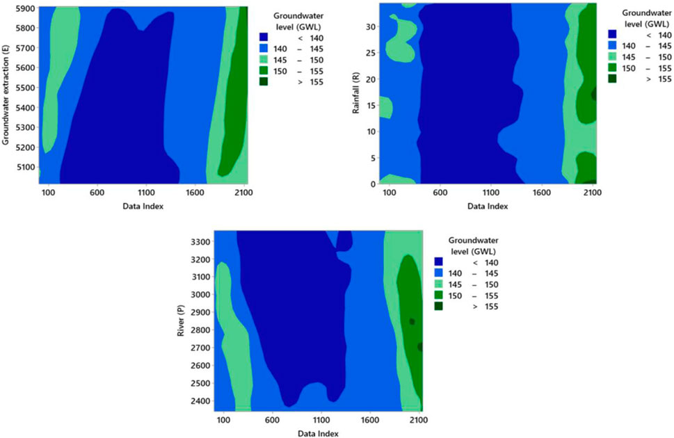
FIGURE 3. Illustration of heat map for input variable for prediction of GWL based on traditional and deep ML (DT, RF, SVM, CNN, GAN, and RNN).

As shown in that figure, 300 data points of the R are in the range of 145 < GWL <150, 1,100 data points of the R are in the range of 140 < GWL <145, and 736 data points of the R are in the range of GWL <140.

Also, 300 data points of the P are in the range of 145 < GWL <150, 1,236 data points of the P are in the range of 140 < GWL <145, and 600 data points of the P are in the range of GWL <140.

To present the Mean and StDev values, we have included the data distribution and data values in Figure 4. As depicted in Figure 4, the histograms visually represent the input/output variables, including E, R, P, and GWL. The distribution of the recorded values is displayed in the histogram for E, which also reveals the frequency of various extraction levels. Similarly, the histogram for R presents the distribution of R values, allowing us to observe the frequency of different precipitation amounts. The histogram for P displays the distribution of P data, providing an overview of the frequency of P measurements. Lastly, the histogram for GWL illustrates the distribution of measured values, giving us an understanding of the frequency of different water level readings. By examining this histogram, we can gain insights into the variability and distribution of GWL, which are crucial for assessing groundwater resources and potential fluctuations (e.g., Kumar and Ahmed, 2003; Ahmadi and Sedghamiz, 2007; Dash et al., 2010).

FIGURE 4

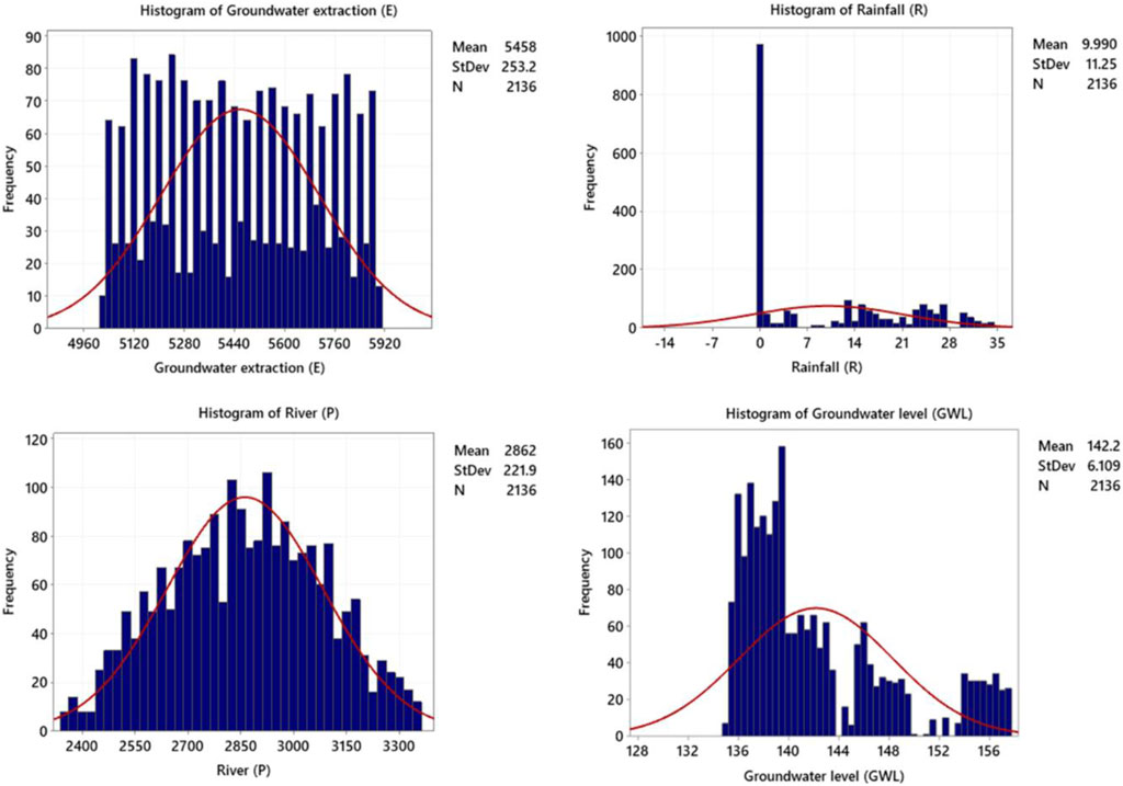
FIGURE 4. Illustration of histograms for input/output variables (groundwater extraction rate (E), rainfall rate (R), river flow rate (P), and groundwater level (GWL)).

4 Discussion of results

In order to predict this critical parameter, DT, RF, SVM, CNN, GAN, and RNN traditional and deep ML algorithms have been used. The reports related to the results of training, testing, validation, and total data are given in Table 6.

TABLE 6

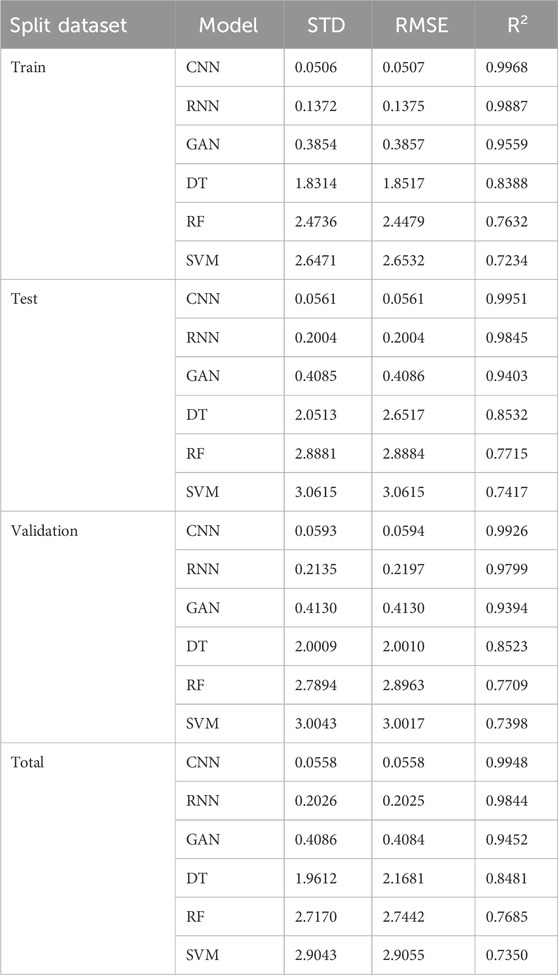
TABLE 6. Statistical reports related to train, test, validation, and total results were used to predict GWL based on traditional and deep ML (DT, RF, SVM, CNN, GAN, and RNN).

This article uses traditional and deep ML (DT, RF, SVM, CNN, GAN, and RNN) methods to predict GWL. The statistical parameters R2, STD, and RMSE are used to evaluate the delivered models in Table 6. After checking the results from Table 6, it is clear that the reports of the CNN model are better than those of the RNN and GAN models. Based on the results shown, it is determined that the values of RMSE and R2 for train, test, validation, and total data are [0.0507, 0.0561, 0.0594, 0.0558] and [0.9968, 0.9951, 0.9926, 0.9948], respectively.

Based on Figure 5, which shows the cross plot between the measured data points and the predicted data, the best AI model for regression can be determined from among the models provided. This figure gives six traditional and deep ML models (DT, RF, SVM, CNN, GAN, and RNN). Based on this figure, a good comparison can be made between the models based on R². Based on the results presented visually for the whole dataset, it is clear that the RNN algorithm has a higher accuracy than the other algorithms. Based on the results shown, it is clear that the accuracy of these algorithms is SVM < RF < DT < GAN < RNN < CNN.

FIGURE 5

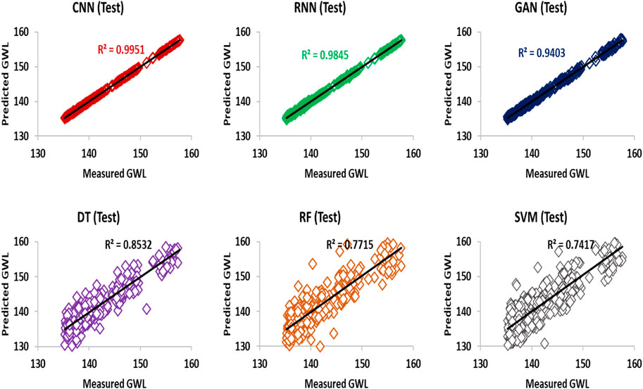
FIGURE 5. Cross plot diagram for prediction of GWL value using new traditional and deep ML algorithms for RF (orange color), SVM (gray color), DT (purple color), CNN (red color), RNN (green color), GAN (blue color) (DT, RF, SVM, CNN, GAN, and RNN).

Figure 6 shows the histogram of the GWL prediction error for three newly developed deep ML algorithms. As shown in the histogram diagram, GWL prediction errors are symmetrically distributed at the zero point, and for the CNN algorithm, this distribution is normal. Its statistical error distribution is either positively or negatively distributed.

FIGURE 6

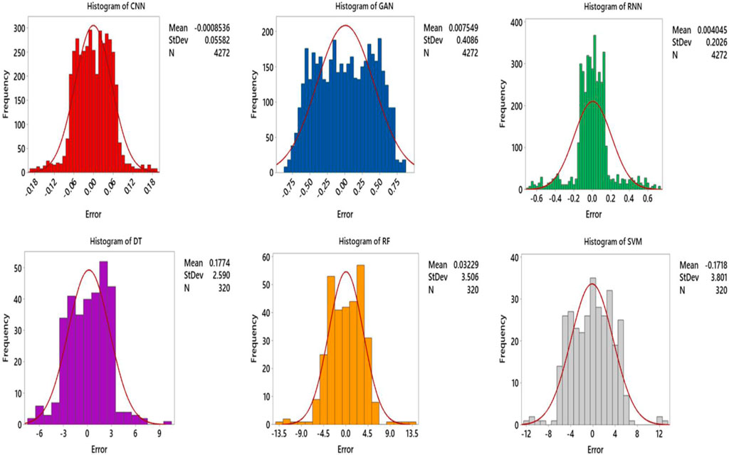
FIGURE 6. Histogram plot to determine the error rate for GWL prediction using deep ML algorithms RF (orange color), SVM (gray color), DT (purple color), CNN (red color), RNN (green color), GAN (blue color) (DT, RF, SVM, CNN, GAN, and RNN).

Based on the data presented in Figure 7, which illustrates the relative error (%) versus data index for GWL prediction using deep ML algorithms RNN, CNN, and GAN, we can analyze the error ranges associated with each algorithm (e.g., Yoon et al., 2011; Banadkooki et al., 2020; Di Nunno and Granata, 2020; Azari et al., 2021). The figure provides valuable insights into the accuracy of the DT, RF, SVM, CNN, GAN, and RNN algorithms by depicting their respective relative error (%) ranges. Upon examining Figure 7, we observe that the error range for the CNN algorithm falls between −0.192 and 0.194. In contrast, the RNN algorithm exhibits an error range of −0.693 to 0.729, while the GAN algorithm spans from −0.850 to 0.850, the DT algorithm exhibits an error range of −8.1936 to 10.4948, and the RF algorithm exhibits an error range of −13.7735 to 14.085. while the SVM algorithm spans from −14.7825 to 15.2825. These error ranges show the magnitude and direction of the relative errors between the predicted and actual GWL values (e.g., Yoon et al., 2011; Marchant et al., 2016). Based on this information, it is concluded that the CNN algorithm outperforms the RNN and GAN algorithms in terms of accuracy. The GWL predictions made by the CNN algorithm exhibit a smaller relative error (%) when compared to the RNN, GAN, DT, RF, and SVM algorithms. Therefore, a comparison of these algorithms reveals that the accuracy ranking is as follows: CNN > RNN > GAN > DT > RF > SVM.

FIGURE 7

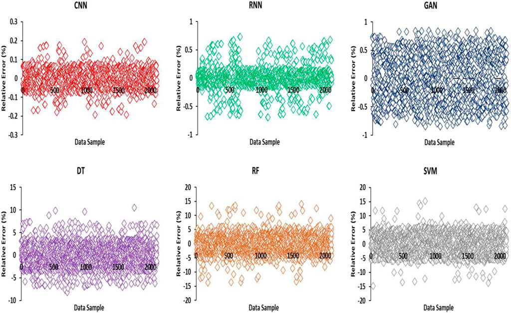
FIGURE 7. Illustration of the relative error (%) versus data index for GWL prediction using deep ML algorithms (RF (orange color), SVM (gray color), DT (purple color), CNN (red color), RNN (green color), GAN (blue color)).

According to the graphical data in Figure 8 and Table 6, which show the RMSE and R2 for GWL prediction utilizing deep ML algorithms (DT, RF, SVM, CNN, GAN, and RNN), the performance accuracy of RMSE and R² yields contrasting results. In other words, as the R² value increases, the corresponding RMSE value decreases. Furthermore, this figure effectively demonstrates the performance accuracy of the algorithms employed for GWL prediction, with the ranking as follows: CNN > RNN > GAN > DT > RF > SVM. Figure 8 provides valuable insights into the relationship between RMSE and R² in the context of GWL prediction. As the R² value increases, it indicates a stronger correlation between the predicted and actual GWL values (e.g., Sakaguchi and Berge, 1998; Seifi et al., 2020; Wu et al., 2023). Consequently, the RMSE value decreases, signifying a smaller average error in the prediction (e.g., Mukherjee and Ramachandran, 2018; Yosefvand and Shabanlou, 2020; Iqbal et al., 2021; Lin et al., 2022; Samantaray et al., 2022). The figure reinforces the conclusion that the CNN algorithm outperforms the RNN and GAN algorithms in terms of accuracy for GWL prediction. The higher R² and lower RMSE values associated with CNN demonstrate its superior performance compared to the other algorithms. Therefore, the comparative analysis suggests the following accuracy ranking: CNN > RNN > GAN > DT > RF > SVM.

FIGURE 8

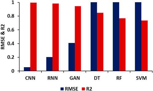
FIGURE 8. Illustration of RMSE and R² for GWL prediction using deep ML algorithms (DT, RF, SVM, CNN, GAN, and RNN).

A comparison of Pearson and Spearman correlation coefficients based on Figure 9 can provide insight into the relationship between input variables and GWL (e.g., Hauke and Kossowski, 2011; Worsa-Kozak et al., 2020; Balacco et al., 2022). The observed negative correlation between groundwater recharge (R and P) and GWL indicates that these input factors yield a negative influence when incorporated into the linear relationship governing GWL or when included in the proportion it affects. In contrast, the observed positive correlation between E and GWL indicates that E has a positive power or direct proportionality when placed in the physical linear relationship of GWL (e.g., Hauke and Kossowski, 2011; Mukherjee and Ramachandran, 2018). The E involves drawing water from underground aquifers for purposes like irrigation, industry, and domestic use (Foster and Chilton, 2003; Worsa-Kozak et al., 2020). This often leads to declining GWL as extraction outpaces natural replenishment from R and infiltration, creating a positive correlation between E and GWL reduction.

FIGURE 9

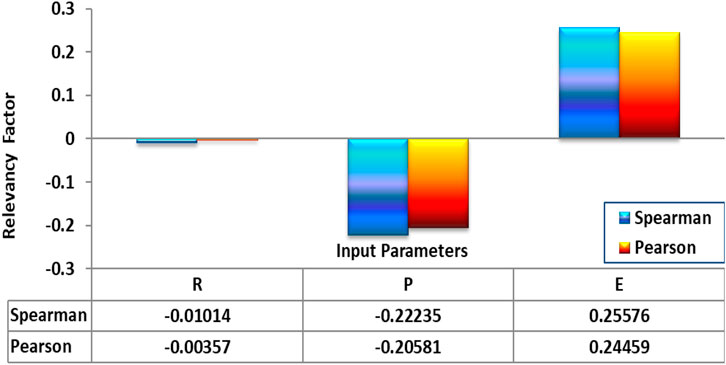
FIGURE 9. Correlation between input and output parameters for Pearson and Spearman equations to predict GWL.

In contrast, P can exhibit a negative correlation with GWL due to stream-aquifer interaction. Elevated GWL can feed P, bolstering their flow, while low GWL prompts P to recharge adjacent aquifers by seeping water into the ground, establishing a dynamic that yields a negative correlation between P and GWL. Given that the Pearson value for R is approximately −0.00357 and close to zero, it can be assumed that this parameter has little effect on GWL. The use of both Pearson and Spearman correlation methods provides a robust analysis of the data, and the results can be used to develop GWL prediction models based on the input variables (Hauke and Kossowski, 2011; Worsa-Kozak et al., 2020). Expressing the relationships between input variables and GWL in Eq. (10) allows quantitative data analysis and facilitates comparison with other studies.

$GWL=\propto \left(E\right)andGWL=\propto \frac{1}{\left(P,R\right)}(10)$

The analysis of the Spearman and Pearson correlation coefficient values indicates that variables P and E have a stronger influence on GWL than variable R. This suggests that E and P flow are more significant factors affecting GWL than R (e.g., Kim et al., 2016; Csáfordi et al., 2017). However, it is important to note that the relative importance of these variables may vary depending on the specific site conditions and hydrological characteristics. The relative contributions of these variables to GWL can be determined with the aid of additional analysis, such as regression modeling, which can also offer insights into the underlying mechanisms causing the observed correlations (Hauke and Kossowski, 2011). The interpretation of the correlation coefficients should also consider the statistical significance of the results as well as the potential for confounding variables or measurement error (Mukherjee and Ramachandran, 2018; Iqbal et al., 2021).

Deep learning’s outstanding capabilities include forecasting crucial GWL characteristics (Sit et al., 2020; Afan et al., 2021; Wunsch et al., 2021). By employing powerful algorithms, these predictions can ensure accurate estimations, meet the water supply needs of the people in the Izeh area, and enhance their quality of life. The AI, including deep learning, has demonstrated its value in predicting GWL parameters. Leveraging these sophisticated algorithms, we can achieve precise predictions, thereby effectively addressing the water supply requirements of the community in Izeh and safeguarding their wellbeing.

5 Limitation

The limitations of this article are the lack of access to additional information about water diversion, evaporation rate, and temperature data in the target area, especially Izeh City. It is recommended that other researchers consider the influence of these parameters due to their considerable availability when predicting GWL. Including these parameters in the prediction model can provide a more accurate estimate of groundwater resources. This is particularly important because various factors, such as evaporation and temperature, affect GWL. Additionally, a similar article has not been published for Izeh City so far, and it has been somewhat challenging to provide data at this wide level.

Furthermore, it is essential to highlight that the effectiveness of CNN algorithms in predicting GWL is enhanced when a substantial number of input variables are employed. In this article, only three parameters were utilized as input variables, leading to the anticipation that augmenting the inputs will likely boost the accuracy of GWL predictions. Hence, it is recommended that researchers to incorporate a greater number of input variables to enhance the algorithm’s accuracy.

6 Conclusion

An extensive 2,136 time series data points dataset has been collected from the Izeh City of Khuzestan province in Iran. The collected data was utilized using the DML technique to effectively predict the GWL in the proximate wellbore regions by means of three input variables: groundwater extraction rate (E), rainfall rate (R), and river flow rate (P). Through analysis, it has been discovered that deep machine learning (DML) algorithms, such as recurrent neural network (RNN), convolutional neural network (CNN), generative adversarial network (GAN), decision tree (DT), random forest (RF), and support vector machine (SVM), which are traditional and deep ML algorithms, can be employed to predict GWL with remarkable precision. Moreover, the correlation coefficient analyses of Pearson and Spearman revealed that the GWL is negatively and indirectly related to the input variables of groundwater recharge (R and P). However, the input variable “E” exhibits a positive correlation with GWL.

Furthermore, the Spearman and Pearson correlation coefficients ascertain that the input variables P and E have a more significant influence on GWL compared to variable R. Considering that the Pearson value for R is approximately −0.00357 and close to zero, it can be inferred that this parameter has little effect on GWL. However, deep learning algorithms possess the capability to select impactful features and eliminate less influential ones. The level of GWL prediction accuracy achieved by the CNN model, applied to all data records in the comprehensive dataset, is impressive: RMSE = 0.0558 and R² = 0.9948. CNN, a cutting-edge deep ML algorithm that is a robust and efficacious ML tool for data point prediction processing, is applied in this study. Its capability to learn and detect patterns in vast datasets makes it an excellent choice for prediction data points with multiple input variables. Some of the advantages of using CNN over DT, RF, SVM, GAN, and RNN algorithms for the prediction of data points include robustness to noise and variability, scalability to handle extensive datasets with multiple input variables, parallelization for rapid processing speeds for real-time and near real-time applications, generalization to learn and identify patterns in data without explicit programming, and fewer outlier data predictions. This research can assist the residents of Izeh City in the Khuzestan province in conserving and managing their water resources and achieving increased crop productivity for the local economy. This approach can be applied to predict GWL in different parts of the world, and it can potentially improve water management in regions facing water scarcity due to global population growth.

Data availability statement

The data analyzed in this study is subject to the following licenses/restrictions: Data can be made available upon reasonable requests for academic purposes through the corresponding authors. Requests to access these datasets should be directed to hamzehghorbani68@yahoo.com.

Author contributions

FF: Conceptualization, Formal Analysis, Funding acquisition, Methodology, Resources, Software, Validation, Visualization, Writing–original draft, Writing–review and editing. HG: Conceptualization, Data curation, Formal Analysis, Funding acquisition, Methodology, Software, Supervision, Validation, Visualization, Writing–original draft, Writing–review and editing. AR: Conceptualization, Funding acquisition, Methodology, Resources, Validation, Visualization, Writing–original draft, Writing–review and editing.

Funding

The author(s) declare that no financial support was received for the research, authorship, and/or publication of this article.

Conflict of interest

The authors declare that the research was conducted in the absence of any commercial or financial relationships that could be construed as a potential conflict of interest.

Publisher’s note

All claims expressed in this article are solely those of the authors and do not necessarily represent those of their affiliated organizations, or those of the publisher, the editors and the reviewers. Any product that may be evaluated in this article, or claim that may be made by its manufacturer, is not guaranteed or endorsed by the publisher.

Footnotes

¹FEFLOW: is a computer program for simulating groundwater flow, mass transfer, and heat transfer in porous and fractured media

²MODFLOW: is the U.S. Geological Survey modular finite-difference flow model, which is a computer code that solves the groundwater flow equation.

³HydroGeoSphere: is a 3D control-volume finite element groundwater model that accounts for surface and subsurface flow, solute and energy transport, and heat transport.

References

Afan, H. A., Ibrahem Ahmed Osman, A., Essam, Y., Ahmed, A. N., Huang, Y. F., Kisi, O., et al. (2021). Modeling the fluctuations of groundwater level by employing ensemble deep learning techniques. Eng. Appl. Comput. Fluid Mech. 15, 1420–1439. doi:10.1080/19942060.2021.1974093

CrossRef Full Text | Google Scholar

Ahmadi, S. H., and Sedghamiz, A. (2007). Geostatistical analysis of spatial and temporal variations of groundwater level. Environ. Monit. Assess. 129, 277–294. doi:10.1007/s10661-006-9361-z

PubMed Abstract | CrossRef Full Text | Google Scholar

Alarsan, F. I., and Younes, M. (2021). Best selection of generative adversarial networks hyper-parameters using genetic algorithm. SN Comput. Sci. 2, 283. doi:10.1007/s42979-021-00689-3

CrossRef Full Text | Google Scholar

Alfarrah, N., and Walraevens, K. (2018). Groundwater overexploitation and seawater intrusion in coastal areas of arid and semi-arid regions. Water 10, 143. doi:10.3390/w10020143

CrossRef Full Text | Google Scholar

Alsaqr, A. M. (2021). Remarks on the use of Pearson’s and Spearman’s correlation coefficients in assessing relationships in ophthalmic data. Afr. Vis. Eye Health 80, 10. doi:10.4102/aveh.v80i1.612

CrossRef Full Text | Google Scholar

Azari, A., Zeynoddin, M., Ebtehaj, I., Sattar, A. M., Gharabaghi, B., and Bonakdari, H. (2021). Integrated preprocessing techniques with linear stochastic approaches in groundwater level forecasting. Acta Geophys. 69 (4), 1395–1411. doi:10.1007/s11600-021-00617-2

CrossRef Full Text | Google Scholar

Azari, M., Rafiei, H., and Akbarzadeh-T, M.-R. (2022). “Robust human movement prediction by completion-generative adversarial networks with huber loss,” in 2022 29th National and 7th International Iranian Conference on Biomedical Engineering (ICBME), Tehran, Iran, Islamic Republic of, December, 2022, 198–204.

CrossRef Full Text | Google Scholar

Azizah, L. M. r., Umayah, S. F., Riyadi, S., Damarjati, C., and Utama, N. A. (2017). “Deep learning implementation using convolutional neural network in mangosteen surface defect detection,” in 2017 7th IEEE International Conference on Control System, Computing and Engineering (ICCSCE), Penang, Malaysia, November, 2017, 242–246.

CrossRef Full Text | Google Scholar

Bakhtiari, M., Boloorani, A. D., Kakroodi, A. A., Rangzan, K., and Mousivand, A. (2021). Land degradation modeling of dust storm sources using MODIS and meteorological time series data. J. Arid Environ. 190, 104507. doi:10.1016/j.jaridenv.2021.104507

CrossRef Full Text | Google Scholar

Balacco, G., Alfio, M. R., and Fidelibus, M. D. (2022). Groundwater drought analysis under data scarcity: the case of the Salento aquifer (Italy). Sustainability 14 (2), 707. doi:10.3390/su14020707

CrossRef Full Text | Google Scholar

Banadkooki, F. B., Ehteram, M., Ahmed, A. N., Teo, F. Y., Fai, C. M., Afan, H. A., et al. (2020). Enhancement of groundwater-level prediction using an integrated machine learning model optimized by whale algorithm. Nat. Resour. Res. 29, 3233–3252. doi:10.1007/s11053-020-09634-2

CrossRef Full Text | Google Scholar

Barzegar, R., Fijani, E., Moghaddam, A. A., and Tziritis, E. (2017). Forecasting of groundwater level fluctuations using ensemble hybrid multi-wavelet neural network-based models. Sci. Total Environ. 599, 20–31. doi:10.1016/j.scitotenv.2017.04.189

PubMed Abstract | CrossRef Full Text | Google Scholar

Bovolo, C. I., Parkin, G., and Sophocleous, M. (2009). Groundwater resources, climate and vulnerability. Environ. Res. Lett. 4, 035001. doi:10.1088/1748-9326/4/3/035001

CrossRef Full Text | Google Scholar

Brunner, P., and Simmons, C. T. (2012). HydroGeoSphere: a fully integrated, physically based hydrological model. Ground water 50, 170–176. doi:10.1111/j.1745-6584.2011.00882.x

CrossRef Full Text | Google Scholar

Csáfordi, P., Szabó, A., Balog, K., Gribovszki, Z., Bidló, A., and Tóth, T. (2017). Factors controlling the daily change in groundwater level during the growing season on the Great Hungarian Plain: a statistical approach. Environ. Earth Sci. 76, 1–16. doi:10.1007/s12665-017-7002-1

CrossRef Full Text | Google Scholar

Dash, J. P., Sarangi, A., and Singh, D. K. (2010). Spatial variability of groundwater depth and quality parameters in the national capital territory of Delhi. Environ. Manag. 45, 640–650. doi:10.1007/s00267-010-9436-z

PubMed Abstract | CrossRef Full Text | Google Scholar

Dehghani, R., and Torabi Poudeh, H. (2022). Application of novel hybrid artificial intelligence algorithms to groundwater simulation. Int. J. Environ. Sci. Technol. 19, 4351–4368. doi:10.1007/s13762-021-03596-5

CrossRef Full Text | Google Scholar

De Winter, J. C. F., Gosling, S. D., and Potter, J. (2016). Comparing the Pearson and Spearman correlation coefficients across distributions and sample sizes: a tutorial using simulations and empirical data. Psychol. methods 21, 273–290. doi:10.1037/met0000079

PubMed Abstract | CrossRef Full Text | Google Scholar

Di Nunno, F., and Granata, F. (2020). Groundwater level prediction in Apulia region (Southern Italy) using NARX neural network. Environ. Res. 190, 110062. doi:10.1016/j.envres.2020.110062

PubMed Abstract | CrossRef Full Text | Google Scholar

Dong, J., and Lin, T. (2019). MarginGAN: adversarial training in semi-supervised learning. Adv. neural Inf. Process. Syst. 32.

Google Scholar

Eriksson, E. (1970). Groundwater time series: an exercise in stochastic hydrology. Hydrology Res. 1, 181–205. doi:10.2166/nh.1970.0012

CrossRef Full Text | Google Scholar

Foster, S. S. D., and Chilton, P. J. (2003). Groundwater: the processes and global significance of aquifer degradation. Philosophical Trans. R. Soc. Lond. Ser. B Biol. Sci. 358 (1440), 1957–1972. doi:10.1098/rstb.2003.1380

PubMed Abstract | CrossRef Full Text | Google Scholar

Franses, P. H., and Van Dijk, D. (2000). Non-linear time series models in empirical finance. Cambridge, United Kingdom: Cambridge University Press.

Google Scholar

Garbin, C., Zhu, X., and Marques, O. (2020). Dropout vs. batch normalization: an empirical study of their impact to deep learning. Multimedia Tools Appl. 79, 12777–12815. doi:10.1007/s11042-019-08453-9

CrossRef Full Text | Google Scholar

Ghobadi, F., and Kang, D. (2023). Application of machine learning in water resources management: a systematic literature review. Water 15, 620. doi:10.3390/w15040620

CrossRef Full Text | Google Scholar

Giordano, M., Cristiano, G., Ishibashi, K., Ambrogio, S., Tsai, H., Burr, G. W., et al. (2019). Analog-to-digital conversion with reconfigurable function mapping for neural networks activation function acceleration. IEEE J. Emerg. Sel. Top. Circuits Syst. 9, 367–376. doi:10.1109/jetcas.2019.2911537

CrossRef Full Text | Google Scholar

Gomes, H. M., Bifet, A., Read, J., Barddal, J. P., Enembreck, F., Pfharinger, B., et al. (2017). Adaptive random forests for evolving data stream classification. Mach. Learn. 106, 1469–1495. doi:10.1007/s10994-017-5642-8

CrossRef Full Text | Google Scholar

Gong, Y., Zhang, Y., Lan, S., and Wang, H. (2016). A comparative study of artificial neural networks, support vector machines and adaptive neuro fuzzy inference system for forecasting groundwater levels near Lake Okeechobee, Florida. Water Resour. Manag. 30, 375–391. doi:10.1007/s11269-015-1167-8

CrossRef Full Text | Google Scholar

Han, T., Pang, J., and Tan, A. C. C. (2021). Remaining useful life prediction of bearing based on stacked autoencoder and recurrent neural network. J. Manuf. Syst. 61, 576–591. doi:10.1016/j.jmsy.2021.10.011

CrossRef Full Text | Google Scholar

Hauke, J., and Kossowski, T. (2011). Comparison of values of Pearson’s and Spearman’s correlation coefficients on the same sets of data. Quaest. Geogr. 30 (2), 87–93. doi:10.2478/v10117-011-0021-1

CrossRef Full Text | Google Scholar

Hay, J. E., and Mimura, N. (2005). Sea-level rise: implications for water resources management. Mitig. Adapt. Strategies Glob. Change 10, 717–737. doi:10.1007/s11027-005-7305-5

CrossRef Full Text | Google Scholar

Hoseini, Y. (2022). Evaluation of WMS model in basins without statistical data in southwestern Iran using Dicken’s experimental method (case study: kuhgel Basin of Khuzestan Province). Appl. Water Sci. 12 (7), 162. doi:10.1007/s13201-022-01685-5

CrossRef Full Text | Google Scholar

Hughes, J. D., Russcher, M. J., Langevin, C. D., Morway, E. D., and McDonald, R. R. (2022). The MODFLOW Application Programming Interface for simulation control and software interoperability. Environ. Model. Softw. 148, 105257. doi:10.1016/j.envsoft.2021.105257

CrossRef Full Text | Google Scholar

Iqbal, N., Khan, A. N., Rizwan, A., Ahmad, R., Kim, B. W., Kim, K., et al. (2021). Groundwater level prediction model using correlation and difference mechanisms based on boreholes data for sustainable hydraulic resource management. IEEE Access 9, 96092–96113. doi:10.1109/access.2021.3094735

CrossRef Full Text | Google Scholar

Jafari, H., Bagheri, R., Forghani, G., and Esmaeili, M. (2015). The consequences of disposing wastewater in an endorheic wetland in southwest Iran. Environ. Monit. Assess. 187, 1–14. doi:10.1007/s10661-015-4560-0

PubMed Abstract | CrossRef Full Text | Google Scholar

Kalantari, N., Pawar, N. J., and Keshavarzi, M. R. (2009). Water resource management in the intermountain Izeh plain, southwest of Iran. J. Mt. Sci. 6, 25–41. doi:10.1007/s11629-009-0212-6

CrossRef Full Text | Google Scholar

Kang, D.-h., So, Y. H., Kim, I. K., Oh, S.-b., Kim, S., and Kim, B.-W. (2017). Groundwater flow and water budget analyses using HydroGeoSphere model at the facility agricultural complex. J. Eng. Geol. 27, 313–322. doi:10.9720/kseg.2017.3.313

CrossRef Full Text | Google Scholar

Kanjo, E., Younis, E. M. G., and Ang, C. S. (2019). Deep learning analysis of mobile physiological, environmental and location sensor data for emotion detection. Inf. Fusion 49, 46–56. doi:10.1016/j.inffus.2018.09.001

CrossRef Full Text | Google Scholar

Kaya, Y. Z., Üneş, F., Demirci, M., Taşar, B., and Varçin, H. (2018). “Groundwater level prediction using artificial neural network and M5 tree models,” in Air and Water Components of the Environment Conference, March, 2018, 195–201.

CrossRef Full Text | Google Scholar

Kecman, V. (2001). Learning and soft computing: support vector machines, neural networks, and fuzzy logic models. Cambridge, Massachusetts, United States: MIT press.

Google Scholar

Khan, J., Lee, E., Balobaid, A. S., and Kim, K. (2023). A comprehensive review of conventional, machine leaning, and deep learning models for groundwater level (GWL) forecasting. Appl. Sci. 13, 2743. doi:10.3390/app13042743

CrossRef Full Text | Google Scholar

Khan, U. T., and Valeo, C. (2016). Dissolved oxygen prediction using a possibility theory based fuzzy neural network. Hydrology Earth Syst. Sci. 20, 2267–2293. doi:10.5194/hess-20-2267-2016

CrossRef Full Text | Google Scholar

Kim, I., Park, D., Kyung, D., Kim, G., Kim, S., and Lee, J. (2016). Comparative influences of precipitation and river stage on groundwater levels in near-river areas. Sustainability 8 (1), 1. doi:10.3390/su8010001

CrossRef Full Text | Google Scholar

Kombo, O. H., Kumaran, S., Sheikh, Y. H., Bovim, A., and Jayavel, K. (2020). Long-term groundwater level prediction model based on hybrid KNN-RF technique. Hydrology 7, 59. doi:10.3390/hydrology7030059

CrossRef Full Text | Google Scholar

Kotsiantis, S. B. (2013). Decision trees: a recent overview. Artif. Intell. Rev. 39, 261–283. doi:10.1007/s10462-011-9272-4

CrossRef Full Text | Google Scholar

Kumar, D., and Ahmed, S. (2003). Seasonal behaviour of spatial variability of groundwater level in a granitic aquifer in monsoon climate. Curr. Sci., 188–196.

Google Scholar

Kumar, D., Roshni, T., Singh, A., Jha, M. K., and Samui, P. (2020). Predicting groundwater depth fluctuations using deep learning, extreme learning machine and Gaussian process: a comparative study. Earth Sci. Inf. 13, 1237–1250. doi:10.1007/s12145-020-00508-y

CrossRef Full Text | Google Scholar

Li, D., Chen, D., Jin, B., Shi, L., Goh, J., and Ng, S.-K. (2019). MAD-GAN: multivariate anomaly detection for time series data with generative adversarial networks. Berlin, Germany: Springer, 703–716.

CrossRef Full Text | Google Scholar

Lin, H., Gharehbaghi, A., Zhang, Q., Band, S. S., Pai, H. T., Chau, K. W., et al. (2022). Time series-based groundwater level forecasting using gated recurrent unit deep neural networks. Eng. Appl. Comput. Fluid Mech. 16 (1), 1655–1672. doi:10.1080/19942060.2022.2104928

CrossRef Full Text | Google Scholar

Ma, J., Liu, H., Shi, Y., and Zhang, H. (2022). “Study on the numerical simulation of groundwater “drainage and recharge” in open pit coal mine based on FEFLOW,” in 2022 8th International Conference on Hydraulic and Civil Engineering: Deep Space Intelligent Development and Utilization Forum (ICHCE), Xi’an, China, November, 2022, 1–8.

Google Scholar

Machiwal, D., and Singh, P. K. (2015). Understanding factors influencing groundwater levels in hard-rock aquifer systems by using multivariate statistical techniques. Environ. Earth Sci. 74 (7), 5639–5652. doi:10.1007/s12665-015-4578-1

CrossRef Full Text | Google Scholar

Mahdavi, P., Kharazi, H. G., Eslami, H., Zohrabi, N., and Razaz, M. (2021). Drought occurrence under future climate change scenarios in the Zard River basin, Iran. Water Supply 21 (2), 899–917. doi:10.2166/ws.2020.367

CrossRef Full Text | Google Scholar

Malakar, P., Mukherjee, A., Bhanja, S. N., Sarkar, S., Saha, D., and Ray, R. K. (2021). Deep learning-based forecasting of groundwater level trends in India: implications for crop production and drinking water supply. ACS ES&T Eng. 1, 965–977. doi:10.1021/acsestengg.0c00238

CrossRef Full Text | Google Scholar

Marchant, B., Mackay, J., and Bloomfield, J. (2016). Quantifying uncertainty in predictions of groundwater levels using formal likelihood methods. J. Hydrology 540, 699–711. doi:10.1016/j.jhydrol.2016.06.014

CrossRef Full Text | Google Scholar

Ming, Y., Cao, S., Zhang, R., Li, Z., Chen, Y., Song, Y., et al. (2017). “Understanding hidden memories of recurrent neural networks,” in 2017 IEEE Conference on Visual Analytics Science and Technology (VAST), Phoenix, AZ, USA, October, 2017, 13–24.

CrossRef Full Text | Google Scholar

Mirsalari, S. A., Sinaei, S., Salehi, M. E., and Daneshtalab, M. (2020). “MuBiNN: multi-level binarized recurrent neural network for EEG signal classification,” in 2020 IEEE International Symposium on Circuits and Systems (ISCAS), Seville, Spain, October, 2020, 1–5.

CrossRef Full Text | Google Scholar

Mohammed, K. S., Shabanlou, S., Rajabi, A., Yosefvand, F., and Izadbakhsh, M. A. (2023). Prediction of groundwater level fluctuations using artificial intelligence-based models and GMS. Appl. Water Sci. 13, 54. doi:10.1007/s13201-022-01861-7

CrossRef Full Text | Google Scholar

Mukherjee, A., and Ramachandran, P. (2018). Prediction of GWL with the help of GRACE TWS for unevenly spaced time series data in India: analysis of comparative performances of SVR, ANN and LRM. J. hydrology 558, 647–658. doi:10.1016/j.jhydrol.2018.02.005

CrossRef Full Text | Google Scholar

Nadiri, A. A., Chitsazan, N., Tsai, F. T. C., and Moghaddam, A. A. (2014). Bayesian artificial intelligence model averaging for hydraulic conductivity estimation. J. Hydrologic Eng. 19, 520–532. doi:10.1061/(asce)he.1943-5584.0000824

CrossRef Full Text | Google Scholar

Nadiri, A. A., Fijani, E., Tsai, F. T. C., and Asghari Moghaddam, A. (2013). Supervised committee machine with artificial intelligence for prediction of fluoride concentration. J. Hydroinformatics 15, 1474–1490. doi:10.2166/hydro.2013.008

CrossRef Full Text | Google Scholar

Nassery, H. R., Alijani, F., and Mirzaei, L. (2009). Environmental characterization of a karst polje: an example from Izeh polje, southwest Iran. Environ. Earth Sci. 59, 99–108. doi:10.1007/s12665-009-0008-6

CrossRef Full Text | Google Scholar

Nayak, P. C., Rao, Y. R. S., and Sudheer, K. P. (2006). Groundwater level forecasting in a shallow aquifer using artificial neural network approach. Water Resour. Manag. 20, 77–90. doi:10.1007/s11269-006-4007-z

CrossRef Full Text | Google Scholar

O’Shea, K., and Nash, R. (2015). An introduction to convolutional neural networks. https://arxiv.org/abs/1511.08458.

Google Scholar

Osman, A. I. A., Ahmed, A. N., Chow, M. F., Huang, Y. F., and El-Shafie, A. (2021). Extreme gradient boosting (Xgboost) model to predict the groundwater levels in Selangor Malaysia. Ain Shams Eng. J. 12, 1545–1556. doi:10.1016/j.asej.2020.11.011

CrossRef Full Text | Google Scholar

Ozer, M. E., Sarica, P. O., and Arga, K. Y. (2020). New machine learning applications to accelerate personalized medicine in breast cancer: rise of the support vector machines. Omics a J. Integr. Biol. 24, 241–246. doi:10.1089/omi.2020.0001

CrossRef Full Text | Google Scholar

Panahi, M., Sadhasivam, N., Pourghasemi, H. R., Rezaie, F., and Lee, S. (2020). Spatial prediction of groundwater potential mapping based on convolutional neural network (CNN) and support vector regression (SVR). J. Hydrology 588, 125033. doi:10.1016/j.jhydrol.2020.125033

CrossRef Full Text | Google Scholar

Pham, Q. B., Kumar, M., Di Nunno, F., Elbeltagi, A., Granata, F., Islam, A. R. M. T., et al. (2022). Groundwater level prediction using machine learning algorithms in a drought-prone area. Neural Comput. Appl. 34, 10751–10773. doi:10.1007/s00521-022-07009-7

CrossRef Full Text | Google Scholar

Pragnaditya, M., Abhijit, M., Bhanja, S. N., Kumar, R. R., Sudeshna, S., and Anwar, Z. (2021). Machine-learning-based regional-scale groundwater level prediction using GRACE. Hydrogeology J. 29, 1027–1042. doi:10.1007/s10040-021-02306-2

CrossRef Full Text | Google Scholar

Priyan, K. (2021). Issues and challenges of groundwater and surface water management in semi-arid regions. Groundw. Resour. Dev. Plan. Semi-Arid Region, 1–17. doi:10.1007/978-3-030-68124-1_1

CrossRef Full Text | Google Scholar

Rajaee, T., Ebrahimi, H., and Nourani, V. (2019). A review of the artificial intelligence methods in groundwater level modeling. J. hydrology 572, 336–351. doi:10.1016/j.jhydrol.2018.12.037

CrossRef Full Text | Google Scholar

Rashidi, M., and Hosseinzadeh, M. M. (2019). The role of sub-basins overlooking the city in the occurrence of urban floods in Izeh (Khuzestan). J. Geogr. Environ. Hazards 8 (1), 25–42. doi:10.22067/geo.v0i0.78855

CrossRef Full Text | Google Scholar

Rathinasamy, M., Khosa, R., Adamowski, J., Ch, S., Partheepan, G., Anand, J., et al. (2014). Wavelet-based multiscale performance analysis: an approach to assess and improve hydrological models. Water Resour. Res. 50, 9721–9737. doi:10.1002/2013wr014650

CrossRef Full Text | Google Scholar

Russo, S. L., and Taddia, G. (2009). Groundwater in the urban environment: management needs and planning strategies. Am. J. Environ. Sci. 5, 494–500. doi:10.3844/ajessp.2009.494.500

CrossRef Full Text | Google Scholar

Samantaray, S., Biswakalyani, C., Singh, D. K., Sahoo, A., and Prakash Satapathy, D. (2022). Prediction of groundwater fluctuation based on hybrid ANFIS-GWO approach in arid Watershed, India. Soft Comput. 26 (11), 5251–5273. doi:10.1007/s00500-022-07097-6

CrossRef Full Text | Google Scholar

Seifi, A., Ehteram, M., Singh, V. P., and Mosavi, A. (2020). Modeling and uncertainty analysis of groundwater level using six evolutionary optimization algorithms hybridized with ANFIS, SVM, and ANN. Sustainability 12 (10), 4023. doi:10.3390/su12104023

CrossRef Full Text | Google Scholar

Sharafati, A., Asadollah, S. B. H. S., and Neshat, A. (2020). A new artificial intelligence strategy for predicting the groundwater level over the Rafsanjan aquifer in Iran. J. Hydrology 591, 125468. doi:10.1016/j.jhydrol.2020.125468

CrossRef Full Text | Google Scholar

Shi, H., Xu, M., and Li, R. (2017). Deep learning for household load forecasting—a novel pooling deep RNN. IEEE Trans. Smart Grid 9, 5271–5280. doi:10.1109/tsg.2017.2686012

CrossRef Full Text | Google Scholar

Singh, A., Patel, S., Bhadani, V., Kumar, V., and Gaurav, K. (2024). AutoML-GWL: automated machine learning model for the prediction of groundwater level. Eng. Appl. Artif. Intell. 127, 107405. doi:10.1016/j.engappai.2023.107405

CrossRef Full Text | Google Scholar

Singh, S. K. (2015). Groundwater arsenic contamination in the Middle-Gangetic Plain, Bihar (India): the danger arrived. Int. Res. J. Environ. Sci. 4 (2), 70–76.

Google Scholar

Singh, S. K., Shirzadi, A., and Pham, B. T. (2021a). Application of artificial intelligence in predicting groundwater contaminants. Water Pollut. Manag. Pract., 71–105. doi:10.1007/978-981-15-8358-2_4

CrossRef Full Text | Google Scholar

Singh, S. K., Shirzadi, A., and Pham, B. T. (2021b). Application of artificial intelligence in predicting groundwater contaminants. Water Pollut. Manag. Pract., 71–105. doi:10.1007/978-981-15-8358-2_4

CrossRef Full Text | Google Scholar

Sit, M., Demiray, B. Z., Xiang, Z., Ewing, G. J., Sermet, Y., and Demir, I. (2020). A comprehensive review of deep learning applications in hydrology and water resources. Water Sci. Technol. 82 (12), 2635–2670. doi:10.2166/wst.2020.369

PubMed Abstract | CrossRef Full Text | Google Scholar

Sun, J., Hu, L., Li, D., Sun, K., and Yang, Z. (2022). Data-driven models for accurate groundwater level prediction and their practical significance in groundwater management. J. Hydrology 608, 127630. doi:10.1016/j.jhydrol.2022.127630

CrossRef Full Text | Google Scholar

Szandała, T. (2021). Review and comparison of commonly used activation functions for deep neural networks. Bio-inspired neurocomputing, 203–224. doi:10.1007/978-981-15-5495-7_11

CrossRef Full Text | Google Scholar

Tao, H., Hameed, M. M., Marhoon, H. A., Zounemat-Kermani, M., Heddam, S., Kim, S., et al. (2022a). Groundwater level prediction using machine learning models: a comprehensive review. Neurocomputing 489, 271–308. doi:10.1016/j.neucom.2022.03.014

CrossRef Full Text | Google Scholar

Tao, H., Hameed, M. M., Marhoon, H. A., Zounemat-Kermani, M., Salim, H., Sungwon, K., et al. (2022b). Groundwater level prediction using machine learning models: a comprehensive review. Neurocomputing 489, 271–308. doi:10.1016/j.neucom.2022.03.014

CrossRef Full Text | Google Scholar

Trefry, M. G., and Muffels, C. (2007). FEFLOW: a finite-element ground water flow and transport modeling tool. Groundwater 45, 525–528. doi:10.1111/j.1745-6584.2007.00358.x

CrossRef Full Text | Google Scholar

Wang, C., Bai, Y., Yuan, H., Liu, J., Fernández-Ontiveros, J. A., Coelho, P. R. T., et al. (2022). J-PLUS: support vector regression to measure stellar parameters. Astronomy Astrophysics 664, A38. doi:10.1051/0004-6361/202243130

CrossRef Full Text | Google Scholar

Wang, J., Lin, J., and Wang, Z. (2017). Efficient hardware architectures for deep convolutional neural network. IEEE Trans. Circuits Syst. I Regul. Pap. 65, 1941–1953. doi:10.1109/tcsi.2017.2767204

CrossRef Full Text | Google Scholar

Wang, S., Shao, J., Song, X., Zhang, Y., Huo, Z., and Zhou, X. (2008). Application of MODFLOW and geographic information system to groundwater flow simulation in North China Plain, China. Environ. Geol. 55, 1449–1462. doi:10.1007/s00254-007-1095-x

CrossRef Full Text | Google Scholar

Wang, Y., Feng, B., and Ding, Y., 2021. DSXplore: optimizing convolutional neural networks via sliding-channel convolutions. 2021 IEEE International Parallel and Distributed Processing Symposium (IPDPS), Portland, OR, USA, May, 2021, pp. 619–628.

CrossRef Full Text | Google Scholar

Wen, X., Feng, Q., Deo, R. C., Wu, M., and Si, J. (2017). Wavelet analysis–artificial neural network conjunction models for multi-scale monthly groundwater level predicting in an arid inland river basin, northwestern China. Hydrology Res. 48, 1710–1729. doi:10.2166/nh.2016.396

CrossRef Full Text | Google Scholar

Worsa-Kozak, M., Zimroz, R., Michalak, A., Wolkersdorfer, C., Wyłomańska, A., and Kowalczyk, M. (2020). Groundwater level fluctuation analysis in a semi-urban area using statistical methods and data mining techniques—a case study in wrocław, Poland. Appl. Sci. 10 (10), 3553. doi:10.3390/app10103553

CrossRef Full Text | Google Scholar

Wu, Z., Lu, C., Sun, Q., Lu, W., He, X., Qin, T., et al. (2023). Predicting groundwater level based on machine learning: a case study of the hebei plain. Water 15 (4), 823. doi:10.3390/w15040823

CrossRef Full Text | Google Scholar

Yamashita, R., Nishio, M., Do, R. K. G., and Togashi, K. (2018). Convolutional neural networks: an overview and application in radiology. Insights into imaging 9, 611–629. doi:10.1007/s13244-018-0639-9

PubMed Abstract | CrossRef Full Text | Google Scholar

Yoon, H., Jun, S. C., Hyun, Y., Bae, G. O., and Lee, K. K. (2011). A comparative study of artificial neural networks and support vector machines for predicting groundwater levels in a coastal aquifer. J. hydrology 396 (1-2), 128–138. doi:10.1016/j.jhydrol.2010.11.002

CrossRef Full Text | Google Scholar

Yosefvand, F., and Shabanlou, S. (2020). Forecasting of groundwater level using ensemble hybrid wavelet–self-adaptive extreme learning machine-based models. Nat. Resour. Res. 29 (5), 3215–3232. doi:10.1007/s11053-020-09642-2

CrossRef Full Text | Google Scholar

Zhang, H., Shi, Z., Wang, G., Sun, X., Yan, R., and Liu, C. (2019). Large earthquake reshapes the groundwater flow system: insight from the water-level response to earth tides and atmospheric pressure in a deep well. Water Resour. Res. 55, 4207–4219. doi:10.1029/2018wr024608

CrossRef Full Text | Google Scholar

Zhang, J., Zhu, Y., Zhang, X., Ye, M., and Yang, J. (2018). Developing a Long Short-Term Memory (LSTM) based model for predicting water table depth in agricultural areas. J. hydrology 561, 918–929. doi:10.1016/j.jhydrol.2018.04.065

CrossRef Full Text | Google Scholar

Ziyari, K., and Latifi, O. (2022). An analysis of land ecological networks in Izeh city using colonial competition algorithm. Urban Struct. Funct. Stud. 9 (30), 127–147. doi:10.22080/USFS.2021.3517

CrossRef Full Text | Google Scholar