Developing a hybrid data-driven and informed model for prediction and mitigation of agricultural nitrous oxide flux hotspots

1 Introduction

Of various atmospheric pollutants, greenhouse-forcing gases (GHGs) such as carbon dioxide and methane are well known, and policymakers on regional and global scales often seek to regulate and limit their emissions. In addition to the regulation of GHGs, global policies such as the Montreal Protocol heavily limited and even halted the usage of ozone-depleting pollutants, in order to terminate the ongoing damage to the ozone layer.

Nitrous oxide (N₂O), however, remains widely unregulated, despite being one of the most prevalent and dangerous anthropogenically emitted GHGs, potentially being 300 times more greenhouse forcing than carbon dioxide (Cassia et al., 2018). In addition to this, N₂O is the largest contributor to ozone depletion in the 21st century and is predicted to stay as such for the next 100 years (Ravishankara et al., 2009). It is also critical that we begin cutting and mitigating emission factors in the present, as positive feedback loops have been found in N₂O emissions in a warmer and wetter climate (Griffis et al., 2017). A reduction in N₂O emissions would be a beneficial for both climate change and atmospheric ozone repair.

Perhaps the cause behind the lack of widespread N₂O discharge control is in its emission sources—roughly 70% of anthropogenic N₂O emissions are from agricultural practices such as fertilizer application (Tian et al., 2020). Various microbes are present in the soil, and as part of their biological pathways, they transform nitrogen between various its different chemical forms. Excess nitrogen content from both artificial and natural chemicals (Thomson et al., 2012) cannot fully undergo all biogeochemical soil processes, and not all nitrate is fully denitrified by soil microbes to nitric oxide or ammonium, and instead produces N₂O, a partially reduced form of nitrogen. Although N₂O is produced in many natural biogeochemical pathways, its emissions are heightened with excess nitrogen application. Other pathways in soil similarly produce N₂O. As food and agricultural demand increases across the world, the usage and application of nitrogen-based fertilizers will similarly increase, and with it, N₂O production.

In particular, N₂O was chosen as a target of this study not only due to its prominence as the third most important GHG, or as the most important ozone depletant, but because its emissions are much more unpredictable than other gases, due to its biological origins. This makes N₂O modeling more nuanced, and requires more advanced techniques than simple machine learning or mathematical modelling.

Notably, the bulk of agricultural N₂O emissions happen during “hot moments” and in “hot spots” (Machado et al., 2021), and being able to predict where and when these high flux events occur is of the utmost importance when considering mitigation measures. It was found that in a grazed pastoral farm, only 3.2% of the farmland contributed to 9.4% of the N₂O emissions (Luo et al., 2017). The ability to predict both where and when these hotspots occur is incredibly important for effective mitigation. Strategies for agricultural emission factor mitigation can be implemented on smaller scales while still being highly effective.

Soil nitrogen dynamics are extremely complex, and many attempts have been made to predict N₂O flux variability, with both machine-learning models and process-based models (PBMs), and with some studies even using both in tandem to make predictions (Joshi et al., 2022; Liu et al., 2022, Saha et al., 202). Popular PBMs have been shown to have specific issues with simulation shortcomings, and are not adaptable to different fields/agriculture without calibration (Wang et al., 2021), while pure machine learning models require large amounts of input data to fit the complex subsoil dynamics.

Hybrid machine learning/PB models perform better than either model individually, however, require either large amounts of data or are non-generalizable for various types of agricultural cultivars and require field-specific input parameters to ensure proper data fitting. In this study we propose an alternative machine learning-based approach for the prediction of N₂O flux over periods of time, utilizing a new type of model in machine learning, the physics-informed neural network (PINN) (Markidis, 2021). PINNs enforce soft constraints on the training of neural networks through modified loss function, and they characteristically require much less data to train than pure data-driven approaches and are easily generalizable across various systems (Raissi et al., 2019). One of the key characteristics of a PINN in terms of data approximation is its ability to predict peaks or future trends that may not be present in data, but are represented in the constraining DEs (Figure 1). This may also allow a PINN to approximate sharp peaks in data that may not be accurately predicted by a traditional neural network.

Figure 1

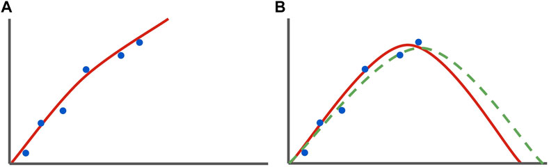
Figure 1. Theoretical example of curve fitting by a classic (left) and an informed (right) model. This Figure (A) shows a set of data (blue), and a curve (red) representing the best solution determined by the machine learning model. The curve fits the best-identified pattern represented only in the raw datapoints. The green perforated curve in (B) illustrates a solution curve predicted by purely natural physical laws. Note that the informed ML model in (B) solves for an NN solution that conforms to natural laws (bends downward after a threshold) while also shifting slightly to accommodate the raw data input. In contrast, the classical model does not have enough data to “understand” that downwards trend, and as such does not represent it in its NN solution.

We first derive a set of differential equations (DEs) to describe the relationship between soil nitrogen compound concentration and N₂O production using a Michaelis-Menten based approximation of soil reaction velocities. We then apply these differential equations to a Multi-Layer Perceptron (MLP) loss function and extensively characterize the network’s performance in determining whether data indicates a high flux event or not. Features of the neural network include various concentrations of compounds found within the soil, as well as data on precipitation and air temperature. The network will be compared pre- and post-loss function modification, based on various statistics, including the ability to explain variance in data, accuracy, and other metrics. In order to determine the performance of the model under smaller training data sets, we also compare both model’s performance after being trained under subsets of the original training data. Using mathematically simple modifications to the loss function expression, we aim to not only show that an informed technique has the potential to solve issues with data availability and model generalization for N₂O predictions, but also that informed techniques like these not only represent a new paradigm in physics based neural network applications, but also in larger scale environmental predictions.

2 Materials and methods

2.1 Data acquisition and preprocessing

The source of data for this study is from a study by Saha et al., 2021 that used soil parameters like chemical concentration and other variables such as precipitation to predict variations in agricultural N₂O flux. The data from the paper was collected from three experiments over an extended period of time (measurements are dated between 2003 and 2017). Data was gathered by automated flux chambers, and measurements were taken 4 times a day and averaged. Flux stations were moved every 10–15 days to minimize spatial variability. Additional details on the experimental location and specific facilities can be found in Saha et al., 2021. A description of features used in the model can be found in Table 1, as well as a description of the model output.

Table 1

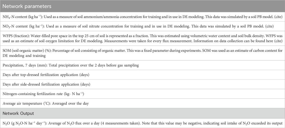
Table 1. Network inputs and the network output descriptions.

This dataset was chosen for this study due to its comprehensive nature, having various climate and soil variables tied to each flux measurement. For future applications of this neural network, many of the major variables used here are easily measured at large scales. This means that when implementing the model proposed here, it is much easier to maintain its operations due to ease of data availability. Notably, many of the variables from the Saha et al. database are relatively simple to integrate into a PINN, due to their correspondence with soil chemical contents that govern N₂O formation.

To prepare data for use in the network, data entries with null values were removed. Additionally, extra data columns present in the original dataset, that were not chosen for use in the network, were removed.

2.2 Neural network architecture and training hyperparameters

The architecture of the neural network (NN) used in this study was a Multi-layer perceptron (MLP). Due to high feature dimensionality, a large number of nodes were used per layer, and multiple hidden layers were used to fit more complex relationships in the data. Both NNs (pre-modification control NN and the informed NN) had 5 total layers, with a 9-node input layer, 3 layers each with 64 nodes, and a final single node layer for regression (Figure 2). In order to minimize coding complexity and streamline NN development, a Python-based Keras/TensorFlow wrapper SciANN (Haghighat and Juanes, 2020) was used to build and train the network. The activation function chosen was Tanh, as it is a nonlinear function that ranges from (−1, 1) and doesn’t suffer from being “stuck” during backpropagation like the sigmoid function (Szandała, 2020).

Figure 2

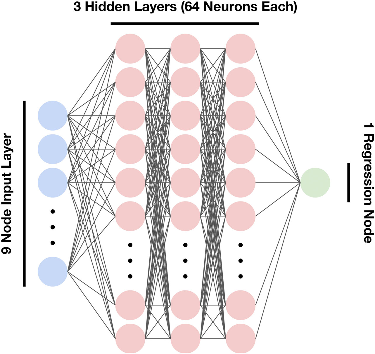
Figure 2. Overview of the neural network architecture. The layers are as follows: 9-dimensional input layer, 3 hidden layers (64 neurons each), 1-dimensional output layer (node).

Training was done using a mini-batch gradient descent, with a set batch size of 128. The learning rate in SciANN was set to 0.001, and the network used the Adam optimizer for gradient descent. Due to a relatively low quantity of data points (2,246 total), a 60:40 train-test split was used to minimize the variance in both the parameter estimates and performance statistics, and neural network training took place over 150 epochs. The random seed used for neural network training was 28.

Due to an imbalanced dataset (only 355 of 2,246 flux events classified as high flux events), the network generally heavily underestimated peaks in the data, lowering both the overall model classification and regression accuracy. In order to combat this, a basic oversampling technique was used. Of the training data in the split, all data points classified as “hotspot” were sampled 3 times each, allowing for a more balanced representation of spikes in the data. This effectively increased the amount of training data by ∼30%.

In order to further test the informed network’s ability to train effectively, many metrics used to characterize models were also used on both models that were only trained on a subset of data. Only 25% of the original training data was randomly sampled for these trials (15% of the total original dataset). Note that the training data for both trials were generated randomly once, and used with both networks to ensure that no bias would occur.

2.3 Loss function modification

Many types of loss functions are used in data-driven neural networks, the most common of which is the mean squared error (MSE) loss function, and is the loss function used in this study. The general form of an MSE loss function is:

$\mathit{arg}\mathit{min}{\mathcal{L}}_{\mathcal{m}\mathcal{s}\mathcal{e}}=\frac{1}{n}{\displaystyle \sum _{i=1}^n}{\left(y_i-\widehat{y_i}\right)}^2(1)$

Where $y_i$ and $\widehat{y_i}$ are the true value of a network output and the predicted value of a network output respectively. The MSE function serves as a simple, non-computationally intensive measure of network performance.

Applying Eq. 1, an ordinary purely data-driven MLP has a loss function of the form:

$ar{g}_{W,b}\mathit{min}\hspace{0.25em}{\mathcal{L}}_{\mathcal{d}\mathcal{a}\mathcal{t}\mathcal{a}}\left(W,b\right)=\frac{1}{n}{\displaystyle \sum _{i=1}^n}{\left(N\left(x_i,y_i,z_i,\dots \right)-\widehat{N}\left(x_i,y_i,z_i,\dots \right)\right)}^2=\frac{1}{n}{\displaystyle \sum _{i=1}^n}{\left(N\left(x_i,y_i,z_i,\dots \right)-{\mathcal{N}}_{\mathcal{N}}\left(W,b,x_i,y_i,z_i,\dots \right)\right)}^2(2)$

Where $N$ and $\widehat{N}$ indicate the true output as a function of the input parameters and the predicted output from a neural network with those same input parameter values respectively. Note that $N$ is equivalently represented as ${\mathcal{N}}_{\mathcal{N}}$, the neural network function with weights ($W$) and biases ($b$) as inputs.

When informing the network, another term is created that accounts for deviation in the neural network from the DEs that constrain it:

$f_{DE}=\frac{\partial N}{\partial x}(\mathrm{3a})$

$ar{g}_{W,b}\mathit{min}\hspace{0.25em}{\mathcal{L}}_{\mathcal{i}\mathcal{n}\mathcal{f}\mathcal{o}}\left(W,b\right)=\frac{1}{n}{\displaystyle \sum _{i=1}^n}{\left(\frac{\partial {\mathcal{N}}_{\mathcal{N},\mathcal{i}}}{\partial x_i}-f_{DE}\right)}^2(\mathrm{3b})$

Where the derivative of the network output with respect to an input parameter $\left(\frac{\partial N}{\partial x}\right)$ is modeled by some function ($f_{DE}$). Note that $f_{DE}$ can be a function of any parameter in the network or of a differential of parameters in the model.

These loss functions from Eqs 2, 3b are then added to generate the final loss function in Eq. 4:

$ar{g}_{W,b}\mathit{min}\hspace{0.25em}{\mathcal{L}}_{\mathcal{t}\mathcal{o}\mathcal{t}\mathcal{a}\mathcal{l}}\left(W,b\right)={\mathcal{L}}_{\mathcal{d}\mathcal{a}\mathcal{t}\mathcal{a}}\left(W,b\right)+{\mathcal{L}}_{\mathcal{i}\mathcal{n}\mathcal{f}\mathcal{o}}\left(W,b\right)=\frac{1}{n}{\displaystyle \sum _{i=1}^n}{\left(N\left(x_i,y_i,z_i,\dots \right)-{\mathcal{N}}_{\mathcal{N}}\left(W,b,x_i,y_i,z_i,\dots \right)\right)}^2+K\frac{1}{n}{\displaystyle \sum _{i=1}^n}{\left(\frac{\partial {\mathcal{N}}_{\mathcal{N},\mathcal{i}}}{\partial x_i}-f_{DE}\right)}^2(4)$

The value of $K$ is added to dictate the relative importance of the physics-based function versus the data-driven loss, although for this study $K$ is set to a value of 1.

This knowledge integration allows for much faster convergence, ensures that the hypothesis set is limited to realistic constraints, and improves the overall accuracy of the model. The model shown in this study does include multiple unknown parameters in its loss function, and these parameters are set as trainable during network training as well. This parameter inversion could also classify the neural network as a supervised learning approach, in contrast to a classical neural network being unsupervised (Cuomo et al., 2022).

The general training pipeline for physics-informed neural network training is shown in Figure 3.

Figure 3

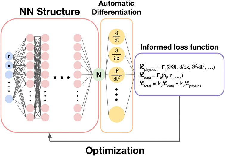
Figure 3. The general training pipeline for a physics informed neural network. After the network is evaluated, the network is differentiated with respect to network parameters. The calculated values for the differentials are then plugged into the physics informed loss function equation and summed with a data-driven loss function term. The loss is then used in the optimization/gradient descent algorithm to adjust the network parameters.

2.4 Derivation of differential equation constraints

Nitrogen in the soil takes upon various forms, and the processes that interchange these nitrogen compounds are extraordinarily intricate. For this reason, the DEs that are used here to model the major processes that produce and consume N₂O are approximations of the complex kinetics that govern soil N₂O flux.

The 3 main processes that most directly affect N₂O soil concentration are nitrification, nitrifier denitrification, and denitrification. All three processes serve to produce N₂O, while denitrification also serves to consume N₂O. In order to simplify kinetic studies, steady-state intermediates (such as nitrite) were not considered for DE derivation. The total rate of production was calculated for N₂O, as well as ammonia/ammonium and nitrate. The chemical reactions that govern the concentrations of the three compounds are shown below:

$N{H}_4^{+}+2O_2\to N{O}_3^{-}+H_{2}O+2H^{+}(\mathrm{5a})$

$2.5N{H}_4^{+}+2.75O_2\to N_{2}O+{0.5NO}_2^{-}+3.5H_{2}O+3H^{+}(\mathrm{5b})$

$2N{H}_4^{+}+2O_2\to N_{2}O+3H_{2}O+2H^{+}(\mathrm{5c})$

$2N{O}_3^{-}+2C{H}_{2}O+2H^{+}\to N_{2}O+C{O}_2+3H_{2}O(\mathrm{5d})$

$N_{2}O+0.5C{H}_{2}O\to N_2+0.5C{O}_2+0.5H_{2}O(5e)$

Equations 5a–5c are the chemical reactions that correspond to the processes of nitrification and nitrifier denitrification, and are large sources of N₂O. The other large source is denitrification, with the incomplete reduction of nitrate to N₂O represented in Eq. 5d, and the major soil sink of N₂O, the complete reduction of N₂O to nitrogen in Eq. 5e.

All of these reactions are catalyzed by soil microbes, and various biological enzymes catalyze these biochemical pathways in cells. As such, all reaction velocities can be expressed as a function of the substrate (reactant) concentrations by the Michaelis-Menten model of enzyme kinetics:

$\frac{d\left[P\right]}{dt}=V_{\mathit{max}}\frac{\left[S\right]}{\left[S\right]+K_m}(6)$

Where $\frac{d\left[P\right]}{dt}$ is the reaction velocity (rate of product formation with respect to time), $\left[S\right]$ is the substrate concentration, $V_{\mathit{max}}$ is the maximum reaction rate, and $K_m$ is a kinetic parameter that is inversely related to the affinity an enzyme has for the substrate.

Using Eq. 6, the rate of formation of each nitrogen-containing compound can be expressed as a function of reactant concentrations:

$\frac{d\left[N{O}_3^{-}\right]}{dt}=v_1\frac{\left[N{H}_4^{+}\right]}{\left[N{H}_4^{+}\right]+k_1}\frac{\left[O_2\right]}{\left[O_2\right]+k_2}-2v_2\frac{\left[N{O}_3^{-}\right]}{\left[N{O}_3^{-}\right]+k_3}\frac{\left[C{H}_{2}O\right]}{\left[C{H}_{2}O\right]+k_4}\frac{I_1}{\left[O_2\right]+I_1}(\mathrm{7a})$

$\frac{d\left[N{H}_4^{+}\right]}{dt}=\frac{d{\left[N{H}_4^{+}\right]}_{prod}}{dt}-v_1\frac{\left[N{H}_4^{+}\right]}{\left[N{H}_4^{+}\right]+k_1}\frac{\left[O_2\right]}{\left[O_2\right]+k_2}-2.5v_3\frac{\left[N{H}_4^{+}\right]}{\left[N{H}_4^{+}\right]+k_5}\frac{\left[O_2\right]}{\left[O_2\right]+k_6}-2v_4\frac{\left[N{H}_4^{+}\right]}{\left[N{H}_4^{+}\right]+k_7}\frac{\left[O_2\right]}{\left[O_2\right]+k_8}\frac{I_2}{\left[O_2\right]+I_2}(\mathrm{7b})$

$\frac{d\left[N_{2}O\right]}{dt}=v_2\frac{\left[N{O}_3^{-}\right]}{\left[N{O}_3^{-}\right]+k_3}\frac{\left[C{H}_{2}O\right]}{\left[C{H}_{2}O\right]+k_4}\frac{I_1}{\left[O_2\right]+I_1}+v_3\frac{\left[N{H}_4^{+}\right]}{\left[N{H}_4^{+}\right]+k_5}\frac{\left[O_2\right]}{\left[O_2\right]+k_6}+v_4\frac{\left[N{H}_4^{+}\right]}{\left[N{H}_4^{+}\right]+k_7}\frac{\left[O_2\right]}{\left[O_2\right]+k_8}\frac{I_2}{\left[O_2\right]+I_2}-v_5\frac{\left[N_{2}O\right]}{\left[N_{2}O\right]+k_9}\frac{\left[C{H}_{2}O\right]}{\left[C{H}_{2}O\right]+k_{10}}(\mathrm{7c})$

$v_{1-5}$ and $k_{1-10}$ are kinetic parameters specific to each reaction, and are set as trainable during the network training.

Although ammonium doesn’t directly have a chemical equation representing it, it’s primary method of formation is decomposition of biological matter or nitrogen fixation. As such, it’s rate of production is treated as being directly proportional to soil organic matter (SOM) (Nishio and Fujimoto, 1989) (Eq. 8):

$\frac{d{\left[N{H}_4^{+}\right]}_{prod}}{dt}=k_{N{H}_4}\left(SOM\right)(8)$

Where $k_{N{H}_4}$ is set as a trainable constant. The data representations of each reactant concentration are as follows: ammonium and nitrate concentration are directly used from the dataset, and oxygen concentration is estimated by Eq. 9:

$\left[O_2\right]=k_{O_2}\left(1-WFPS\right)(9)$

WFPS represents oxygen limitation in soil, and the factor $k_{O_2}$ corrects for proper unit scale. Organic carbon/material concentration is estimated by the SOM content (Eq. 10):

$\left[C{H}_{2}O\right]=k_{C{H}_{2}O}\left(SOM\right)(10)$

It’s important to note the inhibition terms (denoted $I$ in Eqs 7a–7c) added in certain chemical equations, due to some reactions being inhibited by oxygen concentration.

For implementation of the informed loss function, the differentials of the DEs should be the (partial) derivatives of one parameter with respect to another. For loss function implementation in this study, the N₂O concentration is differentiated with respect to ammonium concentration and with respect to nitrate concentration. From calculus, the multivariable chain rule can be used to express a differential as a sum of two chained differentials (Eqs 11a, 11b):

$A=f\left(B\left(t\right),C\left(t\right),P,W,...\right)(\mathrm{11a})$

$\frac{\partial A}{\partial t}=\frac{\partial A}{\partial B}\frac{\partial B}{\partial t}+\frac{\partial A}{\partial C}\frac{\partial C}{\partial t}(\mathrm{11b})$

For ease of integration into the neural network $\left[N_{2}O\right]$ is modeled as a function of $\left[N{H}_4^{+}\right]$ and $\left[N{O}_3^{-}\right]$, with both of those as functions of time. The loss minimization for this is of the form Eq. 12:

${\mathcal{L}}_{\mathcal{i}\mathcal{n}\mathcal{f}\mathcal{o}}=\frac{1}{n}{\displaystyle \sum _{i=1}^n}{\left(\frac{d\left[N_{2}O\right]}{dt}-\left(\frac{\partial \left[N_{2}O\right]}{\partial \left[N{H}_4^{+}\right]}\frac{d\left[N{H}_4^{+}\right]}{dt}+\frac{\partial \left[N_{2}O\right]}{\partial \left[N{O}_3^{-}\right]}\frac{d\left[N{O}_3^{-}\right]}{dt}\right)\right)}^2(12)$

The informed loss function now appears as (Eq. 13):

$ar{g}_{W,b}\mathit{min}\hspace{0.25em}{\mathcal{L}}_{\mathcal{t}\mathcal{o}\mathcal{t}\mathcal{a}\mathcal{l}}\left(W,b\right)=\frac{1}{n}{\displaystyle \sum _{i=1}^n}{\left(\frac{d\left[N_{2}O\right]}{dt}-\left(\frac{\partial \left[N_{2}O\right]}{\partial \left[N{H}_4^{+}\right]}\frac{d\left[N{H}_4^{+}\right]}{dt}+\frac{\partial \left[N_{2}O\right]}{\partial \left[N{O}_3^{-}\right]}\frac{d\left[N{O}_3^{-}\right]}{dt}\right)\right)}^2+\frac{1}{n}{\displaystyle \sum _{i=1}^n}{\left(N\left(x_i,y_i,z_i,\dots \right)-{\mathcal{N}}_{\mathcal{N}}\left(W,b,x_i,y_i,z_i,\dots \right)\right)}^2(13)$

Where $\left[N_{2}O\right]$ is N₂O concentration in soil, assumed to be linearly related to the gaseous flux outside of the soil.

2.5 Initial conditions

Although all constant parameters are set trainable by the neural network, the parameters were initialized with values that were reasonable estimates for their values. The maximum initial velocities were all set to 3.3 μg−N g⁻¹ day⁻¹, the maximum rate of nitrification found in Hokkaido fields (Nishio and Fujimoto, 1989). The half-saturation constants were initially set to 4.816 · 10^–6 mmol L⁻¹, a unit-corrected value from the same study. Inhibition constants were initialized to half of this value, 2.408 − 10^–6 mmol L⁻¹. Although many constants were initially set at the same value, all parameters were allowed to train separately and held various final values post-NN training.

2.6 Data analysis

Data analysis on the initial raw data was performed in Microsoft Excel, after the removal of data points with missing or invalid values. For model characterization and testing, the output testing data from each model was analyzed using the Python library Scikit-learn.

Although the models developed in this study are considered regression models due to the predictions being continuous and numerical, the models were mainly evaluated on their ability to identify data points that indicate a hotspot for N₂O emission. In order to make this data transformation, a threshold value was used to determine whether a numerical prediction indicated a hotspot. The threshold value was carefully chosen based on the percentage of total emissions that occurred from these hotspots, and the percentage of data points that were classified as a high flux event. The former percentage measure was maximized, while the latter measure was minimized.

The first two evaluation criteria used are the R² (as a measure of percent variance explained by the model) and root mean squared error (RMSE) values, shown below, which evaluate models on their performance as numerical regressors.

$R^2=1-\frac{{\displaystyle \sum _{i=1}}{\left(y_i-\widehat{y_i}\right)}^2}{{\displaystyle \sum _{i=1}}{\left(y_i-\overline{y_i}\right)}^2}$

$RMSE=\sqrt{\frac{1}{n}{\displaystyle \sum _{i=1}^n}{\left(y_i-\widehat{y_i}\right)}^2}$

The other metrics used are commonly used benchmarks for binary classification machine learning models. These include type I and II error rates, false discovery rates, overall accuracy, F1 score, and the area under the curve of the receiver operating characteristic curve (AUC-ROC). These common methods of binary classification characterization account for imbalances in true/false classifications, and additionally, the AUC-ROC metric is independent of the chosen threshold value.

$\#offalsepostitives=fp$

$\#offalsenegatives=fn$

$\#oftruepostitives=tp$

$\#oftruenegatives=tn$

$TypeIError=\frac{fp}{fp+tn}$

$TypeIIError=\frac{fn}{tp+fn}$

$FalseDiscoveryRate=\frac{fp}{fp+tp}$

$Accuracy=\frac{tp+tn}{tp+tn+fp+fn}$

$F1Score=\frac{tp}{tp+0.5\left(fp+fn\right)}$

$AUCROC=\int TPR\hspace{0.25em}d\left[FPR\right]$

Other than comparing the models pre- and post-modification by their performance under the same training conditions, the models are compared in their convergence speed (speed of loss function minimization across multiple epochs) and their accuracy and classification under smaller training data sets.

3 Results and discussion

3.1 Data characterization and threshold determination

The full dataset contains a few extremely high-value outliers that heavily skew the data—these are the high-flux events that are significant contributors to the total flux emissions. Approximating these high values is the primary goal of the model, though for classical machine learning models, this task is difficult. This is where the informed loss function guiding the model to a more accurate solution is important.

In order to utilize the regressor models as classifiers, a threshold value had to be chosen in the data. In order to do this, the percentage of total flux above the threshold was plotted with the percentage of data points recognized as positives against the threshold value (Figure 4A). Notably, the threshold was determined after taking into account the full data set, not just the testing or training sets. A theoretical optimal threshold value would minimize the percentage of data points classified as positive, in order to minimize the number of important high flux events to be mitigated. The threshold should also maximize the percentage of the total flux emitted at these hotspots. It’s difficult to derive a quantitative measure that perfectly optimizes this tradeoff, and for this study, the target threshold was simply the threshold value to the nearest tenth that maximized the flux percentage while staying under 16% of data points classified as positive.

Figure 4

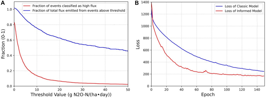
Figure 4. (A) (left). The fraction of total events classified as high flux (red) and fraction of the total flux that was emitted over those events (blue) as a function of the threshold value. Note that the fraction of events classified as high flux is lower than 1 at a threshold value of 0 g N₂O-N ha⁻¹ day⁻¹ due to a large fraction of the dataset containing negative flux events (indicating that N₂O had a greater rate of flow into the soil than out of the soil). The fraction of total flux emitted at a threshold of 0 g N₂O-N ha⁻¹ day⁻¹ appears to be greater than 1 due to the sum of positive fluxes being greater than the sum of all fluxes (positive and negative fluxes). (B) For both models, the total loss is plotted after training each epoch. Loss for the informed model starts at a higher value since the loss function has another term, differential equation loss sum. The classical model trains at a slower rate than the informed model, but shows less spikes in the loss. For the informed model, these small “explosions” in gradient are more common, due to training shifting weights away from a solution that conforms to the informed loss.

The threshold was chosen to be 8.7 g N₂O-N ha⁻¹d⁻¹, with 15.80% of recorded events containing 78.25% of the total flux.

3.2 Convergence speed

An advantage of the informed model is an increase in convergence speed. Figure 4B plots the loss of the model at the conclusion of each epoch.

The total loss for the informed model starts higher than the loss for the classical model, due to the loss function having an additional term and thus gives it a larger loss value. It optimizes much faster than the classical model though, and reaches a more optimal solution in less training time. While it may be inferred that running the model for more epochs may allow the classical loss to reach the same value as the informed loss, as more epochs are run for the model, overfitting begins to occur, and the overall model performance for new data would subsequently worse than the informed model still. Another benefit of the informed model is that it is much more difficult to overfit the training data due to the loss function having an additional non-data-driven term.

3.3 Performance as a regressor

Although these machine learning models are primarily intended for the classification of data, they are fundamentally regressors. As such, the models were evaluated by two key metrics, R² and RMSE. These values were also calculated for models trained with 25% of the original dataset.

The classical model with the full training set had an R² = 0.2978, indicating it explained around 30% of the variation in the data. The model also had a RMSE of 17.03, a relatively high value. Even with oversampling, the classical model’s key weakness was that it could not correctly approximate peaks in the data, often heavily underestimating them (Figure 5). The informed model with the same training parameters and data set had a final R² = 0.8151, meaning that almost 82% of the variance in the data was explained by the model. Additionally, the RMSE of the informed model was 8.74, a large improvement in accuracy. The loss function modification allowed for convergence on a realistic neural network, which improved the model’s testing ability as well.

Figure 5

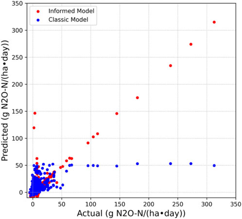
Figure 5. Predicted N₂O fluxes against actual flux measurements plotted for both models above. Examining the plot for the classical model, its key weakness becomes apparent. It cannot predict those extremely high flux events, and instead approximates them as much lower than their actual values. For the classic model, it overpredicts a few low flux events, but generally predicts variation in high flux events with a much higher accuracy.

When the classical model was fed only 25% of the data, effectively making the train/test split 15:40, its RMSE rose to 28.18. The model’s earlier issue of underestimation of large peaks in the data was intensified, and with this training set, the model could only explain 1.7% of variance of N₂O. For this model, this result was expected upon trimming of the data set. The informed model performed better than the classic model with only 25% of the training set, explaining 14.1% of the variation in the data with a RMSE of 21.07.

3.4 Performance as a classifier

Due to the nature of the informed network, it’s difficult to define the network to be a classification model rather than a regression model. The threshold allows for the transformation of the regressed prediction to a classification: a high flux event or not a high flux event.

The various binary classifier statistics used to characterize the classic and informed models with the full training set are summarized in Table 2, and the confusion matrices for each are found in Figures 6A, B.

Table 2

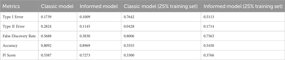
Table 2. Summary of the metrics for the binary classifier models. Models trained on the full dataset along with the models trained with a randomly sampled 25% of the original set are both represented in the table.

Figure 6

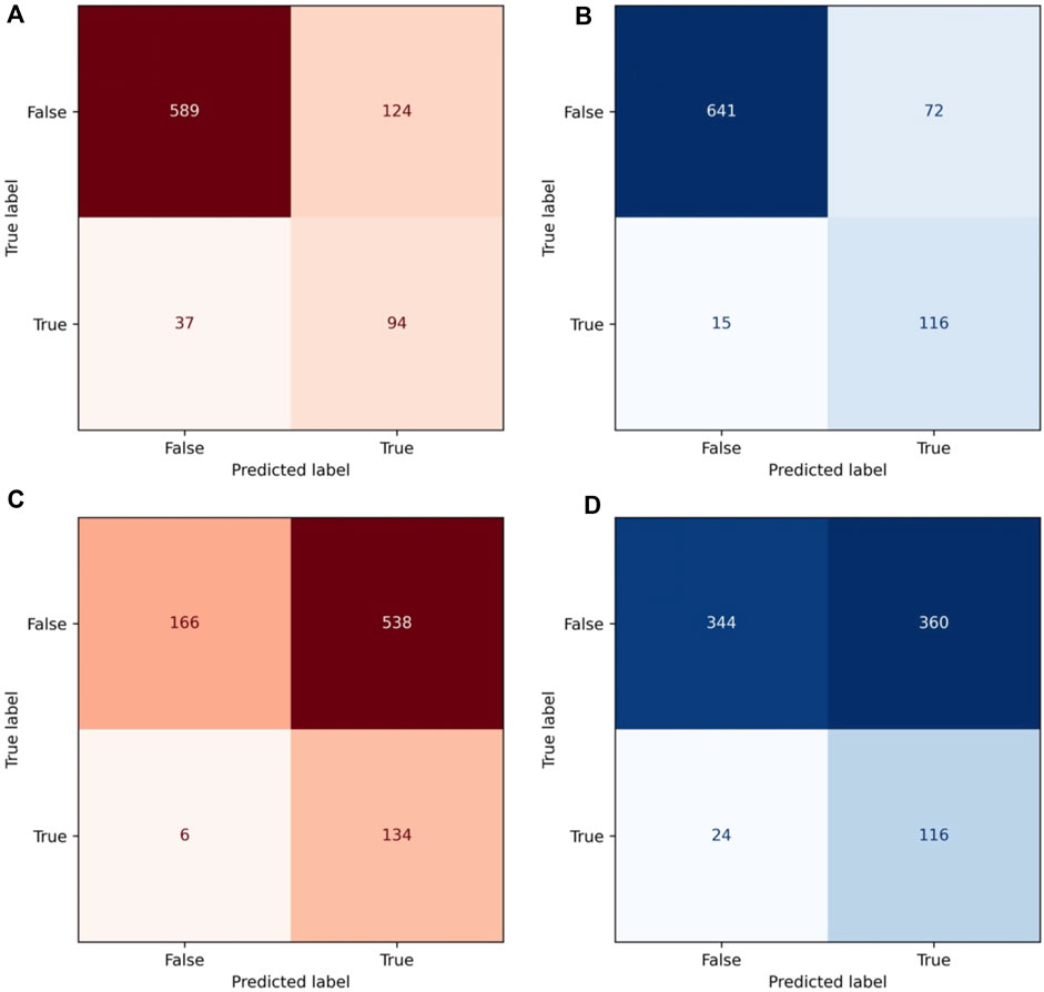
Figure 6. Confusion matrices for both models in both trials. In red: confusion matrix for the classic model with the full training set (A) and the matrix for the classic model with 25% training set (C). In blue: confusion matrix for the informed model with the full training set (B) and the matrix for the informed model with 25% training set (D).

Each of these metrics represents a different type of error or accuracy of a binary classifier. Type I Error is the fraction of false positives of the negatives, and it shows a significant, but not particularly large drop after model modification. This is due to the model’s characteristic behavior of underestimating peaks, but not necessarily overestimating non-high flux events. Type II Error, the fraction of positives classified as negative, had a significant and large drop between models, explained by the informed model being much better at approximating peaks. False discovery rate is another way of looking at this type of error, measuring the fraction of predicted positives that were false. The drop in this statistic is also significant due to the same reasons described earlier.

Accuracy is a measure of the overall accuracy of the model, the fraction of total predictions made correctly. The dataset was overall imbalanced, with the high flux events severely underrepresented. Thus, the prevalent false negatives obtained by the classical model were also underrepresented, and the accuracies for both models are relatively similar. For real-world applications though, the false negative rate should be as minimized as possible in order to mitigate the most total flux.

To combat the skewed nature of accuracy, F1 score was used instead. F1 score is the harmonic mean of the fraction of predicted positives that are true positives and the fraction of real positives that are classified as positive. Since F1 takes into account both, and takes the harmonic mean of the values, it serves as a far better statistic for measuring the accuracy of a binary classification model than the accuracy score. The increase in F1 score between models was extremely significant, meaning that there was a large leap in true accuracy.

These metrics were also used to characterize the network with a smaller training set, containing a randomly sampled 25% of the original training data set. The results for this trial are summarized in Table 2; Figures 6C, D. All measurements show a general increase in accuracy and competency of the model after being informed, and metrics like the overall accuracy, and Type I and Type II errors especially show a large change.

3.5 Importance of performance increase under smaller training set and model interpretability

With expensive measurement and monitoring techniques, especially over long periods of time, it may be hard to gather large data sets for models. In this sense, the significant improvement of the informed model over the classical model under much smaller training sets is extremely important. The physical laws that bind the informed model are able to approximate strong peaks in the output features, making it much more accurate than an ordinary model.

An example of how the model makes peak approximations is shown in the effect of WFPS on N₂O flux. It has been found by Saha et al. that as WFPS reaches roughly 0.7, the N₂O flux shows a sharp and unusual increase. In the enzyme kinetic equations, $\left[O_2\right]$ serves as an inhibitor for many equations, and as WFPS rises, $\left[O_2\right]$ decreases, leading to a general increase in reaction velocity and an increase in gaseous flux.

The informed model accounts for various special patterns like these in the data and allows us to draw conclusions about the underlying reasons for patterns found in the data showing that the informed model has an interpretability that may be lost in classical models.

3.6 The receiver operating characteristics curve metric

Although the threshold value for classification was chosen at a specific point for the metrics above, it’s also helpful to understand how the model performs at varying thresholds. This is where the ROC curve is most valuable. The ROC curve plots the true positive rate against the false positive rate for varying thresholds, and curves that maximize the true positive rate and minimize the false positive rate appear to encompass more of the graph quadrant. The ROC curves for both models are in Figure 7.

Figure 7

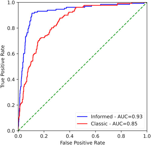
Figure 7. Combined plot of the Receiver Operating Characteristics Curve for the classic model (red) and the informed model (blue). More competent classifiers have curves that tend to hug the top left corner of the plot. As seen, the informed model does this better than the classic model. The area under the curve (AUC) is a quantification of the curves meaning, with AUC values closer to 1 indicating a model of higher accuracy.

The quantification of the ROC curve is given by the area under this curve (AUC-ROC). The AUC-ROC generally varies between 1 and 0.5, with values closer to 1 indicating a better overall model. The AUC-ROC for the classical model is 0.8527, while the informed model had a value of 0.9274. Although the classical model scored well, the seemingly small leaps in the AUC-ROC indicate a large leap in overall model accuracy. The final AUC-ROC score being >0.9 indicates an exceptional ability to classify.

3.7 Model limitations and comparison to existing models

Although the PINN proposed here is much more accurate than previously developed models for N₂O flux, it is limited in certain aspects.

The data used to train the model is not representative of N₂O emissions worldwide, since the sampling locations used for data generation were limited geographically, and in the types of crop field monitored. This may make application of this PINN in particular limited, though it can be trained with additional data as needed.

The concept of the PINN itself was generalized to environmental applications in this study, but the modified loss function used here is not generalized, and will not be accurate for other pollutants released from fields. For future applications of similar techniques, modified loss functions will need to be derived for each of those separately.

No previous model of nitrous flux has used a PINN, though previous models that are either based in machine learning or process-based techniques (PBMs) have been established. The PINN here was only applied to a certain dataset, which had been originally used with a Random Forest machine learning model. The PINN is significantly more accurate in regression than the Random Forest. PBMs, though, require a much larger input than what was used here, requiring variables that constrain nearly every aspect of the system, like sub-soil temperature or soil pH. The PINN doesn’t require as many parameters, and is much more accurate than existing general machine learning techniques.

3.8 The future and other informed machine learning strategies for environmental predictions

When applying this model for use across the world, it is important to acknowledge certain difficulties that may be present for implementation. The most pertinent of which is the issue of non-in situ data collection. There are two key soil chemical contents which are relevant to both the model training and the loss function derivation—soil ammonium and nitrate. These variables have to be constantly gathered for use of this model, and finding a method for doing those at large scales is an important question. One way in which this could be achieved is through satellite spectral index usage. If spectral indices for soil chemical data are extracted, it becomes simple for the model to operate at large scales, continuously.

For a long period of time, physics-informed machine learning was almost entirely applied to only physics-based experiments. Now, however, informed machine learning techniques have been used in various areas, like computational inorganic chemistry (Hautier et al., 2010) and hydrological modeling (Daw et al., 2022). There are many strategies for knowledge integration into neural networks, including training set augmentation and addition, hypothesis set (network architecture), and the strategy used here, learning algorithm integration (von Rueden et al., 2021). Of these, learning algorithm integration is the most generalizable method, and so it was chosen for use here.

With regard specifically to soil biogeochemistry, many chemical processes are regulated by various microorganisms and plants and can be modeled with the same enzyme kinetic approximations described in this study. The hope for this study is that future work can be done using similar algorithms that are described here to introduce a new paradigm for soil and other environmental machine learning applications.

4 Conclusion

In this study, a novel neural network loss function inspired by physics-informed loss functions is derived using enzyme kinetic approximations of soil chemical dynamics to approximate above soil N₂O flux and identify high-flux events that account for 78% of the total flux. The informed network is first measured as a regressor and shows a significant drop in RMSE (∼8.3) as compared to a classical network using the same training data and parameters. A threshold value was then obtained based on the initial dataset to determine a quantitative measure of whether a flux event could be considered high-flux (hotspot) or not. The model was then characterized as a binary classification model, and the informed model was measured to have a much higher F1 score (0.73 vs. 0.54) and AUC ROC value (0.93 vs. 0.85) than the classical model. These scores also showed extreme improvement when the models were trained with only 25% of the initial training set. Differences in the model performances can be accounted for by the reasoning that the informed loss function was able to guide the network to a solution that correctly approximated those high peaks in data using the Michaelis-Menten kinetic model to determine whether a soil nitrogen component had a particularly high rate of formation, or whether a reaction was no longer inhibited by the presence of oxygen (Zhang et al., 2023). The findings shown here represent a new tool that could potentially help in mitigating a very large percentage of agricultural anthropogenic N₂O flux without compromising increasingly important crop yields. We also hope that the new enzyme kinetic based loss function developed in this study represents a new paradigm for studying, understanding, and predicting soil chemical dynamics, combining the flexibility of a classical neural network with the natural laws that govern the system itself.

Data availability statement

The original contributions presented in the study are included in the article/Supplementary material, further inquiries can be directed to the corresponding author.

Author contributions

NV: Conceptualization, Data curation, Investigation, Software, Writing–original draft, Writing–review and editing.

Funding

The author(s) declare that no financial support was received for the research, authorship, and/or publication of this article.

Acknowledgments

We thank Debasish Saha et al for gathering and cleaning the dataset used in this study, and for releasing it for open access.

Conflict of interest

The author declares that the research was conducted in the absence of any commercial or financial relationships that could be construed as a potential conflict of interest.

Publisher’s note

All claims expressed in this article are solely those of the authors and do not necessarily represent those of their affiliated organizations, or those of the publisher, the editors and the reviewers. Any product that may be evaluated in this article, or claim that may be made by its manufacturer, is not guaranteed or endorsed by the publisher.

References

Cassia, R., Nocioni, M., Correa-Aragunde, N., and Lamattina, L. (2018). Climate change and the impact of greenhouse gasses: CO2 and no, friends and foes of plant oxidative stress. Front. Plant Sci. 9, 273. doi:10.3389/fpls.2018.00273

PubMed Abstract | CrossRef Full Text | Google Scholar

Cuomo, S., Di Cola, V. S., Giampaolo, F., Rozza, G., Raissi, M., and Piccialli, F. (2022). Scientific machine learning through physics–informed Neural Networks: where we are and what’s next. J. Sci. Comput. 92 (3), 88. doi:10.1007/s10915-022-01939-z

CrossRef Full Text | Google Scholar

Daw, A., Karpatne, A., Watkins, W. D., Read, J. S., and Kumar, V. (2022). Physics-guided neural networks (PGNN): an application in lake temperature modeling. Knowl. Guid. Mach. Learn., 353–372. doi:10.1201/9781003143376-15

CrossRef Full Text | Google Scholar

Griffis, T. J., Chen, Z., Baker, J. M., Wood, J. D., Millet, D. B., Lee, X., et al. (2017). Nitrous oxide emissions are enhanced in a warmer and wetter world. Proc. Natl. Acad. Sci. 114 (45), 12081–12085. doi:10.1073/pnas.1704552114

PubMed Abstract | CrossRef Full Text | Google Scholar

Haghighat, E., and Juanes, R. (2020). SciANN: a Keras/Tensorflow Wrapper for scientific computations and physics-informed deep learning using artificial neural networks. Comput. Methods Appl. Mech. Eng. 373, 113552. doi:10.1016/j.cma.2020.113552

CrossRef Full Text | Google Scholar

Hautier, G., Fischer, C. C., Jain, A., Mueller, T., and Ceder, G. (2010). Finding nature’s missing ternary oxide compounds using machine learning and density functional theory. Chem. Mater. 22 (12), 3762–3767. doi:10.1021/cm100795d

CrossRef Full Text | Google Scholar

Joshi, D. R., Clay, D. E., Clay, S. A., Moriles-Miller, J., Daigh, A. L., Reicks, G., et al. (2022). Quantification and machine learning based N2O–N and CO2–C emissions predictions from a decomposing rye cover crop. Agron. J. doi:10.1002/agj2.21185

CrossRef Full Text | Google Scholar

Liu, L., Xu, S., Tang, J., Guan, K., Griffis, T. J., Erickson, M. D., et al. (2022). KGML-AG: a modeling framework of knowledge-guided machine learning to simulate agroecosystems: a case study of estimating n₂o emission using data from MESOCOSM experiments. Geosci. Model Dev. 15 (7), 2839–2858. doi:10.5194/gmd-15-2839-2022

CrossRef Full Text | Google Scholar

Luo, J., Wyatt, J., van der Weerden, T. J., Thomas, S. M., de Klein, C. A. M., Li, Y., et al. (2017). Potential hotspot areas of nitrous oxide emissions from grazed pastoral dairy farm systems. Adv. Agron. 205, 205–268. doi:10.1016/bs.agron.2017.05.006

CrossRef Full Text | Google Scholar

Machado, P. V., Farrell, R. E., and Wagner-Riddle, C. (2021). Spatial variation of nitrous oxide fluxes during growing and non-growing seasons at a location subjected to seasonally frozen soils. Can. J. Soil Sci. 101 (3), 555–564. doi:10.1139/cjss-2021-0003

CrossRef Full Text | Google Scholar

Markidis, S. (2021). The old and the new: can physics-informed deep-learning replace traditional linear solvers? Front. Big Data 4, 669097. doi:10.3389/fdata.2021.669097

PubMed Abstract | CrossRef Full Text | Google Scholar

Nishio, T., and Fujimoto, T. (1989). Kinetics of nitrification of various amounts of ammonium added to soils. Soil Biol. Biochem. 22 (1), 51–55. doi:10.1016/0038-0717(90)90059-9

CrossRef Full Text | Google Scholar

Raissi, M., Perdikaris, P., and Karniadakis, G. E. (2019). Physics-informed Neural Networks: a deep learning framework for solving forward and inverse problems involving nonlinear partial differential equations. J. Comput. Phys. 378, 686–707. doi:10.1016/j.jcp.2018.10.045

CrossRef Full Text | Google Scholar

Ravishankara, A. R., Daniel, J. S., and Portmann, R. W. (2009). Nitrous oxide (N2O): the dominant ozone-depleting substance emitted in the 21st Century. Science 326 (5949), 123–125. doi:10.1126/science.1176985

PubMed Abstract | CrossRef Full Text | Google Scholar

Saha, D., Basso, B., and Robertson, G. P. (2021). Machine learning improves predictions of agricultural nitrous oxide (N2O) emissions from intensively managed cropping systems. Environ. Res. Lett. 16 (2), 024004. doi:10.1088/1748-9326/abd2f3

CrossRef Full Text | Google Scholar

Szandała, T. (2020). Review and comparison of commonly used activation functions for deep neural networks. Bio-Inspired Neurocomputing, 203–224. doi:10.1007/978-981-15-5495-7_11

CrossRef Full Text | Google Scholar

Thomson, A. J., Giannopoulos, G., Pretty, J., Baggs, E. M., and Richardson, D. J. (2012). Biological sources and sinks of nitrous oxide and strategies to mitigate emissions. Philosophical Trans. R. Soc. B Biol. Sci. 367 (1593), 1157–1168. doi:10.1098/rstb.2011.0415

PubMed Abstract | CrossRef Full Text | Google Scholar

Tian, H., Xu, R., Canadell, J. G., Thompson, R. L., Winiwarter, W., Suntharalingam, P., et al. (2020). A comprehensive quantification of global nitrous oxide sources and sinks. Nature 586 (7828), 248–256. doi:10.1038/s41586-020-2780-0

PubMed Abstract | CrossRef Full Text | Google Scholar

von Rueden, L., Mayer, S., Beckh, K., Georgiev, B., Giesselbach, S., Heese, R., et al. (2021). Informed machine learning - a taxonomy and survey of integrating prior knowledge into Learning Systems. IEEE Trans. Knowl. Data Eng. 1, 1. doi:10.1109/tkde.2021.3079836

CrossRef Full Text | Google Scholar

Wang, C., Amon, B., Schulz, K., and Mehdi, B. (2021). Factors that influence nitrous oxide emissions from agricultural soils as well as their representation in simulation models: a Review. Agronomy 11 (4), 770. doi:10.3390/agronomy11040770

CrossRef Full Text | Google Scholar