A functional autoregressive approach for modeling and forecasting short-term air temperature

1 Introduction

Air temperature is a crucial meteorological parameter that measures the level of heat or coldness in the air. It is essentially a measure of the kinetic energy, or energy of motion, of the gases that make up the air. The acceleration of the molecular movement of gases corresponds directly to an increase in air temperature (Spiridonov and Ćurić, 2021). Various factors, including solar radiation, atmospheric pressure, and the presence of greenhouse gases, influence this kinetic energy.Air temperature is a fundamental aspect of weather that plays a major role in many areas of our lives including agriculture, energy consumption, public health, and transportation. Accurate air temperature forecasting benefits different stakeholders by providing critical information for decision-making, resource allocation, public safety improvement, and social and economic resilience. The availability of accurate and reliable air temperature forecasts over a short period of time can facilitate farmers, energy, transport, urban planners, and other decision-makers in other sectors to make informed decisions on crop cultivation, energy demand management, traffic management, infrastructure maintenance and many more. Moreover, they help to optimize resource allocation in areas such as energy and water management. For example, utilities can adjust the production and distribution of electricity based on the expected temperature changes. At the same time, water resources managers can plan more effectively for irrigation and water supply management. On the other hand, reliable forecasts of atmospheric temperatures play an important role in public safety, especially in anticipating and preparing for extreme weather events such as heat waves and cold periods. Having accurate forecasts, emergency response agencies, health facilities, and local authorities can take proactive measures to protect vulnerable populations, prevent heat-related diseases, and reduce the impact of extreme temperatures on public health and infrastructure. In addition, forecasting air temperature can contribute to improving social and economic resilience, enabling communities and companies to better anticipate and mitigate the impact of temperature fluctuations. For example, tourism and hospitality companies can adapt their activities according to weather forecasts, while urban planners can design heat-resistant infrastructures to mitigate the impact of urban heat islands (Ostro et al., 2010). Moreover, accurate temperature forecasting plays a significant role in the context of sustainable development goals (SDGs). For example, SDG 13 refers to climate action, which focuses on urgent measures to combat climate change and its impact. A better air temperature forecast is essential to understand climate patterns, predict extreme weather events, and implement strategies to mitigate climate change. In addition, SDG 11, i.e., sustainable cities and communities, aims to promote inclusive, secure, resilient, and sustainable cities. Improvements in air temperature forecasting help urban planners and policymakers design climate-resistance infrastructure, develop heat mitigation strategies, and improve overall city quality of life (United Nations, 2015).

Forecasting hourly air temperature is tricky due to the ever-changing atmospheric factors like sunlight, clouds, wind, and the land’s shape that can significantly affect temperatures. The interaction of these elements can lead to swift temperature changes, making predictions challenging. Moreover, temperature can follow various patterns depending on the location and the time of the year. Air temperature typically follows a daily cycle, with the warmest temperatures occurring in the afternoon and the coolest in the early morning. This phenomenon arises from the earth’s rotation, resulting in varying levels of solar radiation received by different regions of the planet throughout the day. Air temperature also exhibits a seasonal cycle, peaking during summer and reaching its lowest points during winter. This variation is attributed to the earth’s axial tilt, leading to variations in solar radiation received by different regions throughout the year (Yan et al., 2014; Zhu et al., 2022).

Air temperature forecasting is an essential task in many fields of study, and, in the past, many researchers have proposed several methods and techniques to model and forecast air temperature (Asha et al., 2021; Astsatryan et al., 2021; Liu et al., 2021; Ozbek et al., 2021). For instance, Chen et al. (2018) used the seasonal ARIMA (SARIMA) model for predicting monthly mean temperature. The temperature data were collected hourly from a weather station in Nanjing, China, from January 1951 to December 2017. The study evaluated the forecasting accuracy of the proposed model by computing the mean squared error (MSE) of the forecasted values for the period 2015 to 2017. The result concluded that the proposed model demonstrated better forecasting accuracy. Curceac et al. (2019) conducted a study on short-term air temperature prediction using a nonparametric functional (NPF) model and a SARMA model using the air temperature data from the United Arab Emirates (UAE). The data span a period of 29 years, ranging from 1982 to 2010. Forecasts for 1–24 h are obtained from both models, and results are summarized using the MSE, root MSE (RMSE), relative root mean squared error (RMSEr), mean bias (BIAS), and relative mean bias (BIASr). The study’s findings indicated that the SARMA model outperformed during the initial 6 h of a day, while the NPF was more accurate for forecasting durations ranging from 7 to 24 h. Zahroh et al. (2019) presented a study on predicting the daily maximum and minimum air temperatures using the long short-term memory (LSTM) network model and examines the impact of key parameters such as hidden layers, neurons, epochs, and the stochastic gradient algorithm on the accuracy of temperature forecasts. Roy (2020) studied three different models, namely, multilayer perceptron (MLP), LSTM, and a combination of convolutional neural network (CNN) and LSTM to forecast one-day-ahead mean temperature for the next 10 days.

As machine learning techniques are robust and flexible and can account for different features in the data, they are widely used for air temperature forecasting (Agrawal et al., 2012; Kumari et al., 2012; Hossain et al., 2015; Nadtoka and Balasim, 2015; Salcedo-Sanz et al., 2016). For example, Ustaoglu et al. (2008) forecasted the average daily, maximum, and minimum temperature from two meteorological stations, Sakarya and Geyve, in Turkey, ranging from 1989 to 2003, with a total of 5,468 days. For this purpose, three different artificial neural networks (ANN) models, feed-forward back-propagation (FFBP), generalized regression neural network (GRNN), and radial basis function (RBF), were studied. The performance of the ANN models was also compared to the multiple linear regression (MLR) model. The study results suggested that FFBP and RBF models performed superior to GRNN and MLR in predicting daily minimum and maximum temperature. Assuming nonlinearities in the temperature data, Abhishek et al. (2012) used different ANN models with different hidden layers and neurons to forecast the daily maximum temperature for Toronto, Canada, for 1 year. The study found that the ANN model with five hidden layers, 10 or 16 neurons per layer, and ten sigmoid transforms was more effective in predicting weather patterns than only one hidden layer.

The crucial affect of air temperature cannot be ignored in fields like, agriculture, energy, consumption, public health, and transportation. For example, Ali et al. (2013) investigated the relationship between extreme temperatures and electricity demand in Pakistan, finding a positive correlation between the two variables. This implies that as temperatures rise, electricity demand also increases. The study further revealed that this relationship is stronger in urban areas than in rural regions. McFarland et al. (2015) focused on the intricate relationship between rising air temperatures and the performance of the electric grid in the United States (US). As temperatures increase, the grid’s ability to transmit electricity decreases while the demand for electricity increases. From a health perspective, as climate change worsens, its impact on human health becomes more apparent, especially through the combined effects of rising temperatures and worsening air pollution. This results into more heat-related illnesses, respiratory and heart diseases, and the spread of infectious diseases. In addition, it emphasizes that these health problems affect vulnerable populations, such as the elderly, children, and those living in poverty, to a greater extent (Lou et al., 2019). Research in air temperature forecasting is ongoing, driven by the need for more precise and dependable predictions. As statistical models such as time series models get more advanced and data collection technology improves, we can expect more accurate temperature forecasts (Haris et al., 2022; Nandi et al., 2022; Ozbek et al., 2022).

Hourly air temperature forecasting is a challenging task due to the dynamic nature of the atmosphere and the need for precision. Local temperature variations can be significant, and forecasting methods must be able to account for these variations. The traditional forecasting models, including multivariate and univariate, contain many limitations when applied to such datasets. For example, they can only be used to obtain forecasts for a precise time period. In addition, they are less efficient when the data is high-dimensional. The inherent smoothness as well as other properties of the data cannot be used with the classical forecasting models. To overcome these issues, this research proposed a functional time series approach for hourly air temperature forecasts. Within the functional approach, the daily air temperature profile is considered a single functional datum, and unlike the traditional methods, the forecast can be obtained for ultra-short periods. Functional data may or may not be independent of each other and are useful because the derivatives are available for further analysis. Since it is a curve and not like a scalar quantity, being a single datum, the problem of multicollinearity is automatically resolved. It also solves the problem of high dimensionality and removes the noise from the data. Furthermore, it utilizes the inherent smoothness of the data. Functional data analysis (FDA) techniques have been used in various fields, such as bio-statistics, econometrics, engineering, energy, and other sciences (Campbell et al., 2006; Leng and Müller, 2006; Bonner et al., 2014; Jan et al., 2022; Shah et al., 2022). However, the FDA has been less explored in the context of environmental variables forecasting. In addition, neither the proposed model nor the component estimation technique has been used for the air temperature data from the considered site. Furthermore, the proposed model is compared to classical time series models to assess their performance.

The remaining sections of this manuscript are arranged as follows. A brief introduction to the FDA, along with the proposed functional autoregressive model, is provided in Section 2. The general modeling framework and the two competitor models are discussed in Section 3. An empirical investigation of the proposed model and competitors is conducted in Section 4. Finally, the concluding remarks are given in Section 5.

2 Functional Data Analysis

The term “Functional Data Analysis” (FDA) was first introduced by Ramsay in 1982 (Ramsay, 1982) and several traditional statistical tools have been adapted and extended to suit the framework of the FDA (Ferraty, 2006). The FDA is a way of looking at data that are curves, shapes, or patterns rather than just discrete values. Instead of thinking about data as discrete points, like dots on a graph, FDA treats data as curves or functions. This is a convenient way of dealing with information that changes smoothly over time or space (Ramsay and Silverman, 2005).

In general, functional data is gathered on discrete points; however, the frequency of collected data is often very high, and thus, they are easily converted to functional objects. Typically represented by curves, the functional data is constructed using a suitable basis functions system. A system of basis functions denoted as y(j), is defined as a collection of functions that can be expressed as a linear combination of coefficients C_k and basis functions ϕ_k, i.e.,

$y\left(j\right)={\displaystyle \sum _{k=1}^K}{C}_k{\varphi }_k\left(j\right),j\in J(1)$

where C_k represents the coefficients matrix, and ϕ_k represents the known basis functions. The number of basis functions used to construct the functions is an important issue in the FDA. A penalized residual sum of squares criterion is generally employed to determine the optimal number of basis functions. This criterion balances the smoothness of the curve and avoids an inadequate fit to the data. The argument values j are the discretized points where the function is evaluated in the J domain (Ramsay and Silverman, 2005). For simplicity, the notation (j) will be dropped from the function where the notion is clear.

One of the commonly used basis functions is called the Fourier basis functions which are generally employed when dealing with periodic data. The functions are constructed by linearly combining sine and cosine functions of increasing order and can be expressed mathematically as

$y\left(j\right)=c_0+c_1\sin \omega j+c_2\cos \omega j+c_3\sin 2\omega j+c_4\cos 2\omega j+\cdots (2)$

where c₀ is a constant term and c₁, c₂, …, c_k represent the coefficients associated with K basis functions. Here, the number of basis functions is always odd due to including one constant term. The parameter ω specifies the period as 2π/a where a represents the periodicity of the series. An example of a Fourier basis function with k = 10 is plotted in Figure 1.

Figure 1

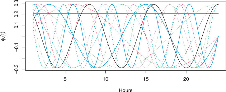
Figure 1. Fourier basis functions with k = 10 and a constant basis function.

2.1 Functional autoregressive model

The functional autoregressive model (FAR) is a statistical technique that helps us to understand how curves change over time when studying functional time series (FTS). It is the extension of the traditional autoregressive (AR) model but in a functional framework. The FAR model assumes that the current state of the function depends on its own past state. This research work used the FAR model of order one within the framework of a Hilbert space $\mathcal{H}$. This approach provides the inherent structure of our data, where observations are not discrete values but dynamic functions evolving over time.

The model is defined within a separable Hilbert space $\mathcal{H}$ with the inner product ⟨⋅, ⋅⟩ and the generating norm ‖⋅‖. For specificity, we focus on the Hilbert space L² [0, 1], although our considerations readily extend to other L²-spaces. A sequence $Y_t,t\in \mathbb{N}$, of Hilbert-random variables, is termed an Autoregressive Hilbertian Process of order 1 (ARH (1)) or FAR(1) if it is strictly stationary and satisfies

$Y_t-\mu =\psi \left(Y_{t-1}-\mu \right)+{\epsilon }_n\text{for\hspace{0.17em}}n\in \mathbb{N}(3)$

where Y_t represents functions in L² [0, 1], ɛ_n is a strong $\mathcal{H}$-white noise with zero mean and finite second moment $(E{‖{\epsilon }_n‖}^2<\infty )$, ψ denotes a bounded linear operator, and μ is the functional mean of the process (Bosq, 2000). For simplicity, μ is assumed to be zero, though this may not be the case in practical applications. The primary advantage of this model is its capability to forecast Y_t+1 using ψ(Y_t). The autoregressive operator ψ: L² [0, 1] → L² [0, one] is supposed to be a bounded linear operator. The following section describes the estimation of the operator ψ within the Hilbert space $\mathcal{H}$.

2.1.1 Estimation of the operator ψ

In estimating the autoregressive operator, ψ within the FAR model, specific assumptions must be addressed to ensure a stationary solution. In particular, two key assumptions are crucial for establishing the existence of such a solution. The first assumption is the presence of an integer, s₀ ≥ 1 such that $\Vert {\psi }^{s0}{\Vert }_L<1$. The second assumption requires the existence of a > 0 and 0 < b < 1 such that ‖ψ^s‖_L ≤ ab^s for all j ≥ 0. Under certain conditions, these assumptions guarantee the existence of a unique strictly stationary solution, as demonstrated in (Bosq, 2000).

It is crucial to emphasize that the estimation of ψ cannot rely on likelihood due to the non-existence of the Lebesgue measure in non-locally compact spaces, and the concept of density is unavailable for functional data. Instead, the classical method of moments is employed. The estimation of ψ is performed as ψ = CΓ⁻¹, where Γ = E (Y_t ⊗ Y_t) and C = E (Y_t ⊗ Y_t+1) represents the covariance and cross-covariance operators of the process, and ⊗ is the Kronecker product. The estimates of these operators are denoted as $\widehat{\mathrm{\Gamma }}$ and $\widehat{C}$, respectively.

Without loss of generality, it is assumed that the mean of the process E (Y_t) = 0 is known. The sample versions of the covariance and cross-covariance operators, denoted as $\widehat{\mathrm{\Gamma }}$ and $\widehat{C}$, are given by:

$\widehat{\mathrm{\Gamma }}=\frac{1}{t}{\displaystyle \sum _{t=0}^t}{Y}_t\otimes Y_t$

and

$\widehat{C}=\frac{1}{t}{\displaystyle \sum _{t=0}^{t-1}}{Y}_t\otimes Y_{t+1}$

The covariance operator Γ possesses key properties, such as being symmetric, positive definite, and compact. It is decomposable into eigenvalues λ_l and ν_l, respectively. However, Γ⁻¹ is not a bounded operator. To overcome this limitation, a practical solution is introduced, involving the use of the m most significant empirical functional principal components (EFPCs) as surrogates for unknown population principal components. This leads to the expression:

${\widehat{\mathrm{\Gamma }}}^{-1}\left(y\right)={\displaystyle \sum _{z=1}^m}{\widehat{\lambda }}_z^{-1}⟨y,{\widehat{\nu }}_z⟩{\widehat{\nu }}_z={\widehat{\mathrm{\Gamma }}}^{†}\left(y\right).$

Transitioning to the context of the scalar autoregressive process with one lag, FAR(1), a relation emerges when multiplying the equation by Y_t as

$Y_t\otimes Y_{t+1}=Y_t\otimes \left(\psi Y_t\right)+Y_t\otimes {ϵ}_{t+1}=\psi Y_t\otimes Y_t+Y_t\otimes {ϵ}_{t+1}.$

Taking into account the definitions of covariance and cross-covariance operators within the framework of FAR(1) and accounting for the vanishing of the ϵ term when expectations are considered, we can express the relationships as follows:

$C=\psi \mathrm{\Gamma }\text{and}\psi =C{\mathrm{\Gamma }}^{-1}.$

The estimation of ψ is then defined as:

${\widehat{\psi }}_t\left(y\right)=\frac{1}{t-1}{\displaystyle \sum _{k=1}^{t-1}}{\displaystyle \sum _{z=1}^m}{\displaystyle \sum _{i=1}^m}{\widehat{\lambda }}_z^{-1}⟨y,{\widehat{\nu }}_z⟩⟨Y_k,{\widehat{\nu }}_z⟩⟨Y_{k+1},{\widehat{\nu }}_i⟩{\widehat{\nu }}_i.$

This expression is obtained by incorporating an additional smoothing step on Y_t+1 and ${\widehat{\nu }}_z$. Notably, the empirical eigenfunctions are recognized for their asymptotic convergence to the population eigenfunctions.Once the estimator $\widehat{\psi }$ of the population parameter ψ is obtained, it becomes crucial to assess its optimality in accurately estimating the true parameter regarding the FAR parameter ψ. Didericksen et al. (2012) demonstrated that the proposed predictor is best in terms of the MSE and Mean Absolute Error (MAE). This is evident as the prediction error of this estimator is similar to that of the unfeasible predictor ψ(y), given by a suitably chosen m.

3 Modeling framework

This section describes the general modeling framework used for the prediction and understanding of the temporal dynamics of hourly air temperature. In addition, it also provides the details about the competing models, i.e., ARIMA and VAR, that are used in this study.

3.1 The model

This research focuses on the crucial task of one-day-ahead hourly air temperature forecasting which is a significant challenge due to the inherent complexities of atmospheric dynamics. These complexities encompass daily and yearly seasonality, non-stationarity, non-linearity, and diverse influencing factors. To accurately capture them in the model, the air temperature series is partitioned into deterministic and stochastic components and are modeled separately. To be more precise, let S_t,j represents an air temperature for day $t(t\in \mathbb{N})$ and hour j (j = 1, …, 24). Then, the dynamics of this series can be modeled as

$S_{t,j}=D_{t,j}+Y_{t,j}(4)$

where D_t,j comprises of deterministic components and Y_t,j represents the stochastic component of the series.

The deterministic component captures predictable patterns like daily and annual seasonalities. One way to deal with daily seasonality is to treat each hour series separately which is adopted in this study (Lisi and Shah, 2020). On the other hand, the annual seasonality A_t,j is modeled and forecasted by using a smooth function of time. Mathematically, it can be written as

$D_{t,j}=f\left(A_{t,j}\right)(5)$

where the function f represents a smooth function of time estimated through cubic smoothing splines. Generally, cross-validation techniques are used to select the number of knots when fitting the cubic smoothing splines (Eilers and Marx, 2010). The stochastic component accounts for unpredictable fluctuations and residual behavior. Once the deterministic component is modeled and forecasted, the stochastic component is obtained as

$\begin{array}{l}\hfill Y_{t,j}=S_{t,j}-{\widehat{D}}_{t,j}\\ \hfill Y_{t,j}=S_{t,j}-{\widehat{A}}_{t,j}.\end{array}$

The stochastic component is modeled and forecasted through the proposed FAR(1) and two competing models given in Section 3.2. In the case of FAR(1), the component Y_t,j is first converted to daily functional trajectories using Eq 1 and the model is applied to functional profiles. In the case of the VAR model, the stochastic component Y_t,j is used as a vector of 24 variables, whereas each hourly series is treated independently in the case of ARIMA. Once both components are estimated, the final forecast is obtained by combining the individual forecasts as

${\widehat{S}}_{t+1,j}={\widehat{D}}_{t+1,j}+{\widehat{Y}}_{t+1,j}(6)$

3.2 Competing models

This section describes two competing classical time series models whose results are compared with the proposed FAR model.

3.2.1 Vector autoregressive model (VAR)

The VAR model is an effective tool for examining the dynamic changes of multiple time series variables over time. It was first proposed by Christopher Sims and Thomas Sargent in the 1980s and has become widely used as it can capture complex relationships between different variables Sargent (1984). The VAR model assumes that the present value of each variable is impacted by its past values as well as the past values of all other variables within the system. The VAR model of order “p” is represented as follows.

${\mathbf{Y}}_t=\alpha +{\displaystyle \sum _{r=1}^p}{\psi }_r{\mathbf{Y}}_{t-r}+{ϵ}_t(7)$

where Y_t represents a vector of time series variables at time t, α is a vector of constants (intercepts), ψ represents the coefficient matrices for lag p, and ϵ_t is the vector of error terms at time t.For the estimation of parameters, techniques such as the ordinary least squares (OLS) or the maximum likelihood (ML) are generally employed. Note that for fitting a VAR model, all variables included in the time series model must be stationary. The order “p” of a VAR model is selected using different information criteria and cross validation approaches. In a VAR model, the total number of estimated coefficients are K + K²∗p, where K represents the number of coefficients for the intercepts, and K²∗p represents the number of coefficients for the lagged values of each variable up to the order “p”.

3.2.2 Autoregressive integrated moving average (ARIMA) models

The ARIMA models, also known as the Box-Jenkins models, are statistical forecasting methods that have been widely used for time series forecasting. In the context of time series analysis, the ARIMA models stand as a foundation, providing a flexible framework for predicting and understanding data that changes over time. Developed by George Box and Gwilym Jenkins in the 1970s, ARIMA models have gained widespread recognition for their ability to capture underlying patterns and trends in a wide range of time series data (Box et al., 2015).

An ARIMA model contains three components: autoregression, differencing, and moving average. The AR component of the ARIMA model captures the notion that the current value of the time series is affected by its past values and is achieved through a linear combination of past values, with the parameter “p” representing the order of the AR term, indicating the number of lagged values incorporated into the prediction equation. Stationarity is a fundamental requirement for ARIMA models to produce reliable forecasts. However, many times series data exhibit non-stationary behavior, meaning their statistical properties, such as mean and variance, vary over time. Differencing transforms non-stationary data into a stationary series by eliminating trends and seasonalities. The order of differencing “d” indicates how many times the data needs to be differenced to achieve stationarity. Finally, the MA component accounts for the influence of past errors on the current value of the time series. It suggests that the accuracy of current predictions can be enhanced by considering the discrepancies between past predictions and the actual observed values. The order of the MA term “q” determines the number of past errors considered when constructing the prediction equation (Shumway et al., 2000).The ARIMA (p,d,q) model can be expressed mathematically as follows.

$Y_t^d={\displaystyle \sum _{r=1}^p}{\psi }_r{Y}_{t-r}^d+{\displaystyle \sum _{i=1}^q}{\varphi }_i{\epsilon }_{t-i}+{\epsilon }_t(8)$

where $Y_t^d$ represents the d-th difference of the time series Y at time t, $Y_{t-r}^d$ is the lagged and differenced value of the time series Y at time t-1, ψ_r (r = 1,2,…,p) and ϕ_i (i = 1,1,2,…,q) are the parameter of AR and MA, respectively, and ${\epsilon }_t\sim \mathcal{N}$(0, ${\sigma }_{\epsilon }^2$). The orders “p” and “q” are determined using information criteria or by analyzing the autocorrelation function (ACF) and partial autocorrelation function (PACF) of a stationary time series. The model parameters are generally estimated through the MLE approach.

4 Modeling and forecasting air temperature

This section provides an empirical application of the proposed modeling framework using a real dataset. Before going into details, a brief description of the dataset is given as under.

4.1 Data description

The research work used an hourly air temperature dataset collected from Islamabad, Pakistan. The dataset is collected through sensors installed at different location in Islamabad and an average value has been reported for each hour (Power, 2022). Hourly measurements capture the dynamic nature of air temperature changes, offering a more comprehensive picture than daily or monthly averages. No missing observations are present within the dataset, ensuring the integrity and reliability of the data for models training and evaluation. The dataset spans over 5-year period, ranging from 1 January 2018, to 31 December 2022, encompasses 43,824 individual observations. The dataset is plotted in Figure 2, where one can see the patterns and variations in the air temperature throughout the years. The red line distinguishes between the model estimation and the out-of-sample forecasting periods.

Figure 2

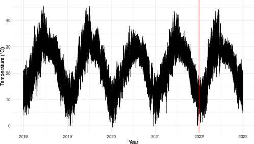
Figure 2. Hourly air temperature time series. The red line distinguishes between model estimation and out-of-sample forecasting periods.

The summary statistics listed in Table 1 provide a comprehensive overview of the hourly temperature data. The table shows that the minimum temperature recorded is −0.45 c°, indicating the presence of lower extreme values. The first quartile (Q1) is 14.54 c° and the median at 22.50 c° provides insights into the central tendency, showcasing that at least 25% of the data falls below 14.54 c° and 50% falls below 22.50 c°. The mean temperature is 21.78 c°, indicating the average value. The third quartile (Q3) at 28.61 c° signifies that at least 75% of the data falls below this point. The maximum temperature recorded is 45.51 c°, indicating the presence of higher extreme values. The variability in the dataset is reflected in the variance, calculated at 80.30404, and the standard deviation, which is 8.961,252 c°, indicates a moderate level of variability.

Table 1

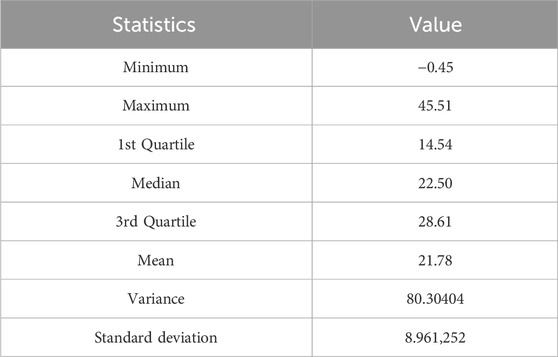
Table 1. Descriptive statistics for hourly air temperature in Islamabad.

4.2 Out-of-sample forecasting

To achieve accurate hourly air temperature forecasting, the dataset was divided into training and testing sets utilizing 80/20 splits. More precisely, from 1 January 2018, to 31 December 2021 (35,064 observations covering 1,461 days) the data points were used for training various forecasting models. The remaining 20%, i.e., from 1 January 2021, to 31 December 2022 (8,760 observations, covering 365 days) served as a hold-out set for evaluating one-day-ahead out-of-sample forecasting performance for each model.

To compare the forecasting accuracy of the models, three different types of error metrics are used in the research work including MAE, RMSE, and mean absolute percentage error (MAPE) (Bibi et al., 2021). The MAE, also known as the mean absolute deviation (MAD), is determined by averaging the absolute differences between the forecasts and the actual values at corresponding time points. In mathematical terms, it is represented as follows.

$\begin{array}{l}\hfill \text{MAE}=\text{mean}\left(\left|S_{t,j}-{\widehat{S}}_{t,j}\right|\right)\end{array}$

where S_t,j is the observed and ${\widehat{S}}_{t,j}$ is the one-day-ahead forecast, for j = 1, …, 24 and t = 1, 2, …, 365. The MAPE is calculated by averaging the absolute deviation divided by the corresponding observed value, multiplied by 100. It is a relative error metric, indicating the extent of error observed in the forecast relative to the actual value. The mathematical expression for the MAPE is written as

$\begin{array}{l}\hfill \text{MAPE}=\text{mean}\left(\left|\frac{S_{t,j}-{\widehat{S}}_{t,j}}{S_{t,j}}\right|\right)\times 100.\end{array}$

On the other hand, the RMSE is a commonly used metric for measuring the average magnitude of the errors between predicted and actual values. It is an extension of MSE and provides a more interpretable result by taking the square root of the average squared differences. Mathematically, the RMSE is defined as

$\begin{array}{l}\hfill \text{RMSE}=\sqrt{\text{mean}{(S_{t,j}-{\widehat{S}}_{t,j})}^2}.\end{array}$

The one-day-ahead out-of-sample air temperature forecasting results are listed in Table 2. These results indicate that the proposed modeling framework efficiently forecasts air temperature as it produces relatively low errors for each model. Comparing the three models, it is evident that the proposed FAR model outperforms the other two models across all metrics. The proposed FAR model achieved an MAE, MAPE, and RMSE of 1.0852, 6.115, and 1.5178, respectively, which are lower than the MAE, MAPE, and RMSE of 1.1075, 6.1320, and 1.5660, respectively of the VAR model, as well as 1.1022, 6.1198, and 1.5535, respectively of the ARIMA model.

Table 2

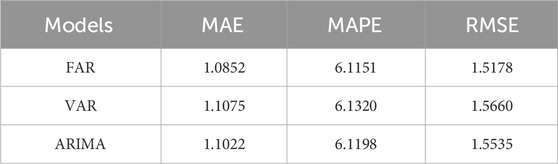
Table 2. One-day-ahead out-of-sample forecasting errors for FAR, VAR, and ARIMA models.

To investigate the performance of each model more deeply, one-day-ahead out-of-sample forecasting errors for each hour are calculated for each model and the results are listed in Table 3. The table indicates that the forecasting errors generally vary throughout the day. The forecasting errors, in general, are low in the initial hours of the day and are high during the final hours. In the initial hours, the performance of the VAR model is slightly better than that of the proposed FAR model. For example, the VAR model achieved the lowest MAE, MAPE, and RMSE values of 0.2744, 0.2022, and 1.5639 respectively in the first hour of the day, which is slightly better than the MAE, MAPE, and RMSE values (0.3611, 0.2556, and 1.9209, respectively) of the proposed model. However, as the day progresses, the proposed model produced better results compared to the VAR and ARIMA models, by providing lower values of MAE, MAPE, and RMSE. Note that both multivariate (FAR and VAR) models perform relatively better than the univariate (ARIMA) model. These findings can be easily noticed in Figure 3 where the hour-specific MAPE values are depicted for each model.

Table 3

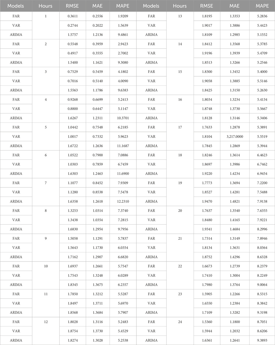
Table 3. Hour specific forecasting errors using FAR, VAR, and ARIMA models.

Figure 3

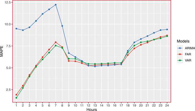
Figure 3. Hour-specific MAPE values for FAR, VAR, and ARIMA models.

The one-day-ahead forecasting errors are summarized month-wise and listed in Table 4. These results indicate that the proposed model performs better, outperforming the ARIMA and VAR models in most months. The errors are relatively higher in the winter and are lower in the summer. In September, the proposed model achieved the lowest MAE, MAPE, and RMSE values of 0.8671, 0.6106, and 2.3199, respectively, outperforming both the VAR and ARIMA models. However, in January, the VAR model outperforms the proposed model, achieving lower MAE, MAPE, and RMSE values of 1.3845, 1.0592, and 13.1341, respectively. Moreover, it is noteworthy that the ARIMA model consistently performs the worst across all months. For a visual illustration of these results, the month-specific MAPE is plotted in Figure 4. Finally, it is worth mentioning that all computations were performed using the R programming environment (R Core Team, 2023) run on an Intel(R)-Core(TM) i7-4770 CPU running at 3.40 GHz.

Table 4

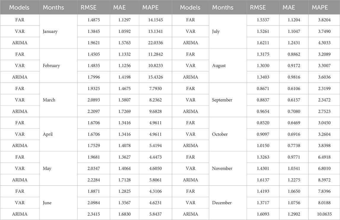
Table 4. Monthly Forecast Errors for Air Temperature using FAR(1), VAR, and ARIMA models.

Figure 4

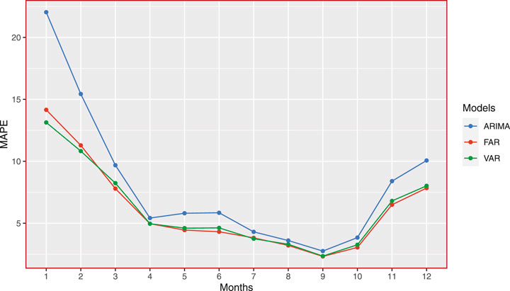
Figure 4. Month-specific MAPE values for FAR, VAR, and ARIMA models.

5 Conclusion

Air temperature is a fundamental aspect of weather that plays a significant role in diverse areas of our lives, and thus, its accurate forecast is crucial. However, an air temperature time series is comprised of different deterministic and stochastic variations that make forecasting challenging. This research work proposes a functional data approach to forecast one-day-ahead air temperature. Moreover, the component estimation technique, which divides the data into deterministic and stochastic components, is used to accurately predict the temperature series dynamics. The deterministic part of the series is modeled and forecasted using smoothing splines, whereas FAR, ARIMA, and VAR models are used for the stochastic component. For empirical assessment, air temperature data for Islamabad (Pakistan) are collected and one-day-ahead out-of-sample forecasting results for a complete year are summarized using MAE, MAPE, and RMSE.The results indicated that the proposed component estimation procedure is efficient in forecasting air temperature. In addition, the functional model, i.e., the FAR model, further improves the forecasting accuracy compared to ARIMA and VAR models, resulting in lower out-of-sample forecasting errors. Finally, the multivariate models, VAR and FAR, outperform ARIMA, demonstrating their effectiveness in predicting air temperature.

Despite the valuable insights obtained from this study, recognizing its limitations is important. The current research work considers only parametric (linear) models. In addition, the dataset is used only from one location. As the current study does not account for the effects of exogenous variables in the model, it would be interesting to see their impact on forecasting air temperature using the current approach in the future. Moreover, the proposed model can be compared with machine learning approaches, generally known as nonlinear models, in a future study. Furthermore, the performance of the proposed approach can be assessed by conducting a study on other site datasets.

Data availability statement

Publicly available datasets were analyzed in this study. This data can be found here: https://power.larc.nasa.gov/data-access-viewer/.

Author contributions

IS: Conceptualization, Investigation, Methodology, Supervision, Writing–original draft. PM: Conceptualization, Formal Analysis, Validation, Writing–review and editing. SA: Data curation, Project administration, Software, Visualization, Writing–review and editing. OA: Funding acquisition, Resources, Validation, Writing–original draft.

Funding

The author(s) declare that financial support was received for the research, authorship, and/or publication of this article. Open Access funding was received for the research provided by Università degli Studi di Padova/University of Padua, Open Science Committee.

Conflict of interest

The authors declare that the research was conducted in the absence of any commercial or financial relationships that could be construed as a potential conflict of interest.

The reviewer (SMMR) declared a past co-authorship with the authors IS and SA to the handling editor.

Publisher’s note

All claims expressed in this article are solely those of the authors and do not necessarily represent those of their affiliated organizations, or those of the publisher, the editors and the reviewers. Any product that may be evaluated in this article, or claim that may be made by its manufacturer, is not guaranteed or endorsed by the publisher.

References

Abhishek, K., Singh, M., Ghosh, S., and Anand, A. (2012). Weather forecasting model using artificial neural network. Procedia Technol. 4, 311–318. doi:10.1016/j.protcy.2012.05.047

CrossRef Full Text | Google Scholar

Agrawal, A., Kumar, V., Pandey, A., and Khan, I. (2012). An application of time series analysis for weather forecasting. Int. J. Eng. Res. Appl. 2, 974–980.

Google Scholar

Ali, M., Iqbal, M. J., and Sharif, M. (2013). Relationship between extreme temperature and electricity demand in Pakistan. Int. J. Energy Environ. Eng. 4, 36. doi:10.1186/2251-6832-4-36

CrossRef Full Text | Google Scholar

Asha, J., Santhosh kumar, S., and Rishidas, S. (2021). “Forecasting performance comparison of daily maximum temperature using arma based methods,” in Journal of physics: conference series (Bristol, United Kingdom: IOP Publishing), 1921, 012041. doi:10.1088/1742-6596/1921/1/012041

CrossRef Full Text | Google Scholar

Astsatryan, H., Grigoryan, H., Poghosyan, A., Abrahamyan, R., Asmaryan, S., Muradyan, V., et al. (2021). Air temperature forecasting using artificial neural network for ararat valley. Earth Sci. Inf. 14, 711–722. doi:10.1007/s12145-021-00583-9

CrossRef Full Text | Google Scholar

Bibi, N., Shah, I., Alsubie, A., Ali, S., and Lone, S. A. (2021). Electricity spot prices forecasting based on ensemble learning. IEEE Access 9, 150984–150992. doi:10.1109/access.2021.3126545

CrossRef Full Text | Google Scholar

Bonner, S. J., Newlands, N. K., and Heckman, N. E. (2014). Modeling regional impacts of climate teleconnections using functional data analysis. Environ. Ecol. statistics 21, 1–26. doi:10.1007/s10651-013-0241-8

CrossRef Full Text | Google Scholar

Bosq, D. (2000) Linear processes in function spaces: theory and applications, 149. Springer Science and Business Media.

Google Scholar

Box, G. E., Jenkins, G. M., Reinsel, G. C., and Ljung, G. M. (2015) Time series analysis: forecasting and control. John Wiley and Sons.

Google Scholar

Campbell, K., McKay, M. D., and Williams, B. J. (2006). Sensitivity analysis when model outputs are functions. Reliab. Eng. Syst. Saf. 91, 1468–1472. doi:10.1016/j.ress.2005.11.049

CrossRef Full Text | Google Scholar

Chen, P., Niu, A., Liu, D., Jiang, W., and Ma, B. (2018). “Time series forecasting of temperatures using sarima: an example from nanjing,” in IOP conference series: materials science and engineering (Bristol, United Kingdom: IOP Publishing), 394, 052024. doi:10.1088/1757-899x/394/5/052024

CrossRef Full Text | Google Scholar

Curceac, S., Ternynck, C., Ouarda, T. B., Chebana, F., and Niang, S. D. (2019). Short-term air temperature forecasting using nonparametric functional data analysis and sarma models. Environ. Model. Softw. 111, 394–408. doi:10.1016/j.envsoft.2018.09.017

CrossRef Full Text | Google Scholar

Didericksen, D., Kokoszka, P., and Zhang, X. (2012). Empirical properties of forecasts with the functional autoregressive model. Comput. Stat. 27, 285–298. doi:10.1007/s00180-011-0256-2

CrossRef Full Text | Google Scholar

Eilers, P. H., and Marx, B. D. (2010). Splines, knots, and penalties. Wiley Interdiscip. Rev. Comput. Stat. 2, 637–653. doi:10.1002/wics.125

CrossRef Full Text | Google Scholar

Ferraty, F. (2006) Nonparametric functional data analysis. Springer.

Google Scholar

Haris, M. D., Adytia, D., and Ramadhan, A. W. (2022). “Air temperature forecasting with long short-term memory and prophet: a case study of Jakarta, Indonesia,” in 2022 international conference on data science and its applications (ICoDSA) (IEEE), 251–256.

CrossRef Full Text | Google Scholar

Hossain, M., Rekabdar, B., Louis, S. J., and Dascalu, S. (2015). “Forecasting the weather of Nevada: a deep learning approach,” in 2015 international joint conference on neural networks (IJCNN) (IEEE), 1–6.

CrossRef Full Text | Google Scholar

Jan, F., Shah, I., and Ali, S. (2022). Short-term electricity prices forecasting using functional time series analysis. Energies 15, 3423. doi:10.3390/en15093423

CrossRef Full Text | Google Scholar

Kumari, K. A., Boiroju, N. K., Ganesh, T., and Reddy, P. R. (2012). Forecasting surface air temperature using neural networks. Int. J. Math. Comput. Appl. Res. 3, 65–78.

Google Scholar

Leng, X., and Müller, H.-G. (2006). Classification using functional data analysis for temporal gene expression data. Bioinformatics 22, 68–76. doi:10.1093/bioinformatics/bti742

PubMed Abstract | CrossRef Full Text | Google Scholar

Lisi, F., and Shah, I. (2020). Forecasting next-day electricity demand and prices based on functional models. Energy Syst. 11, 947–979. doi:10.1007/s12667-019-00356-w

CrossRef Full Text | Google Scholar

Liu, Y., Ortega-Farías, S., Tian, F., Wang, S., and Li, S. (2021). Estimation of surface and near-surface air temperatures in arid northwest China using landsat satellite images. Front. Environ. Sci. 9, 791336. doi:10.3389/fenvs.2021.791336

CrossRef Full Text | Google Scholar

Lou, J., Wu, Y., Liu, P., Kota, S. H., and Huang, L. (2019). Health effects of climate change through temperature and air pollution. Curr. Pollut. Rep. 5, 144–158. doi:10.1007/s40726-019-00112-9

CrossRef Full Text | Google Scholar

McFarland, J., Zhou, Y., Clarke, L., Sullivan, P., Colman, J., Jaglom, W. S., et al. (2015). Impacts of rising air temperatures and emissions mitigation on electricity demand and supply in the United States: a multi-model comparison. Clim. Change 131, 111–125. doi:10.1007/s10584-015-1380-8

CrossRef Full Text | Google Scholar

Nadtoka, I., and Balasim, M. A.-Z. (2015). Mathematical modelling and short-term forecasting of electricity consumption of the power system, with due account of air temperature and natural illumination, based on support vector machine and particle swarm. Procedia Eng. 129, 657–663. doi:10.1016/j.proeng.2015.12.087

CrossRef Full Text | Google Scholar

Nandi, A., De, A., Mallick, A., Middya, A. I., and Roy, S. (2022). Attention based long-term air temperature forecasting network: altf net. Knowledge-Based Syst. 252, 109442. doi:10.1016/j.knosys.2022.109442

CrossRef Full Text | Google Scholar

Ostro, B., Rauch, S., Green, R., Malig, B., and Basu, R. (2010). The effects of temperature and use of air conditioning on hospitalizations. Am. J. Epidemiol. 172, 1053–1061. doi:10.1093/aje/kwq231

PubMed Abstract | CrossRef Full Text | Google Scholar

Ozbek, A., Sekertekin, A., Bilgili, M., and Arslan, N. (2021). Prediction of 10-min, hourly, and daily atmospheric air temperature: comparison of LSTM, ANFIS-FCM, and ARMA. Arabian J. Geosciences 14, 622. doi:10.1007/s12517-021-06982-y

CrossRef Full Text | Google Scholar

Ozbek, A., Yildirim, A., and Bilgili, M. (2022). Deep learning approach for one-hour ahead forecasting of energy production in a solar-pv plant. Energy Sources, Part A Recovery, Util. Environ. Eff. 44, 10465–10480. doi:10.1080/15567036.2021.1924316

CrossRef Full Text | Google Scholar

Power, N. (2022). Data access viewer. Available at: https://power.larc.nasa.gov/data-access-viewer (Last accessed 11.

Google Scholar

Ramsay, J. O. (1982). When the data are functions. Psychometrika 47, 379–396. doi:10.1007/bf02293704

CrossRef Full Text | Google Scholar

Ramsay, J. O., and Silverman, B. W. (2005) Fitting differential equations to functional data: principal differential analysis. Springer.

Google Scholar

R Core Team (2023) R: a language and environment for statistical computing. Vienna, Austria: R Foundation for Statistical Computing.

Google Scholar

Roy, D. S. (2020). Forecasting the air temperature at a weather station using deep neural networks. Procedia Comput. Sci. 178, 38–46. doi:10.1016/j.procs.2020.11.005

CrossRef Full Text | Google Scholar

Salcedo-Sanz, S., Deo, R., Carro-Calvo, L., and Saavedra-Moreno, B. (2016). Monthly prediction of air temperature in Australia and New Zealand with machine learning algorithms. Theor. Appl. Climatol. 125, 13–25. doi:10.1007/s00704-015-1480-4

CrossRef Full Text | Google Scholar

Sargent, T. J. (1984). Autoregressions, expectations, and advice. Am. Econ. Rev. 74, 408–415.

Google Scholar

Shah, I., Muhammad, I., Ali, S., Ahmed, S., Almazah, M. M., and Al-Rezami, A. (2022). Forecasting day-ahead traffic flow using functional time series approach. Mathematics 10, 4279. doi:10.3390/math10224279

CrossRef Full Text | Google Scholar

Shumway, R. H., Stoffer, D. S., and Stoffer, D. S. (2000) Time series analysis and its applications, 3. Springer. doi:10.1007/978-1-4757-3261-0

CrossRef Full Text | Google Scholar

Spiridonov, V., and Ćurić, M. (2021) Air temperature. Cham: Springer International Publishing, 73–86.

CrossRef Full Text | Google Scholar

United Nations (2015) Transforming our world: the 2030 agenda for sustainable development. New York, United States: Department of Economic and Social Affairs Sustainable Development, 16301.

Google Scholar

Ustaoglu, B., Cigizoglu, H., and Karaca, M. (2008). Forecast of daily mean, maximum and minimum temperature time series by three artificial neural network methods. Meteorol. Appl. 15, 431–445. doi:10.1002/met.83

CrossRef Full Text | Google Scholar

Yan, H., Fan, S., Guo, C., Wu, F., Zhang, N., and Dong, L. (2014). Assessing the effects of landscape design parameters on intra-urban air temperature variability: the case of beijing, China. Build. Environ. 76, 44–53. doi:10.1016/j.buildenv.2014.03.007

CrossRef Full Text | Google Scholar

Zahroh, S., Hidayat, Y., Pontoh, R. S., Santoso, A., Sukono, F., and Bon, A. (2019). “Modeling and forecasting daily temperature in bandung,” in Proceedings of the international conference on industrial engineering and operations management, 406–412.

Google Scholar

Zhu, Y., Zhi, X., Lyu, Y., Zhu, S., Tong, H., Mamtimin, A., et al. (2022). Forecast calibrations of surface air temperature over xinjiang based on u-net neural network. Front. Environ. Sci. 10, 1011321. doi:10.3389/fenvs.2022.1011321

CrossRef Full Text | Google Scholar