Consequences of Lack of Parameterization Invariance of Non-informative Bayesian Analysis for Wildlife Management: Survival of San Joaquin Kit Fox and Declines in Amphibian Populations

1. Introduction

Hierarchical models, also known as state-space models, mixed effects models or mixture models, have proved to be extremely useful for modeling and analyzing ecological data (e.g., Bolker, 2008; Kery and Schaub, 2011). Although these models can be analyzed using the likelihood methods (Lele et al., 2007, 2010), the Bayesian approach is the most advocated approach for such models. Many researchers even name hierarchical models as “Bayesian models” (Parent and Rivot, 2013). Of course, there are no Bayesian models or frequentist models. There are only statistical models that we fit to the data using either the Bayesian approach or the frequentist approach. The subjectivity of the Bayesian approach is bothersome to many scientists (Efron, 1986; Dennis, 1996) and hence the trend is to use the non-informative, also called vague or objective, priors instead of the subjective priors provided by an expert. These non-informative priors purportedly “let the data speak” and do not bias the conclusions with the subjectivity inherent in the subjective priors. It has been claimed that Bayesian inferences based on non-informative priors are similar to likelihood inference (e.g., Clark, 2005, p. 3, 5) although such a result has never been rigorously established.

The fact is that it is not even clear what a non-informative prior really means. There are many different ways to construct non-informative priors (Press, 2003, Chapter 5). The most commonly used non-informative priors are either the uniform priors or the priors with very large variances spreading the probability mass almost uniformly over the entire parameter space. These priors have been criticized on computational grounds (e.g., Natarajan and McCulloch, 1998) because they can inadvertently lead to improper posterior distributions. Link (2013) shows similar problems with using uniform prior on the population size when fitting capture-recapture models. However, how does one explain that a uniform prior on probability of success in a Binomial experiment represents non-information but a uniform prior on the population size does not? Gelman (2006) discusses similar computational problems associated with the non-informative priors for variance components and concludes uniform prior is, in fact, a good choice and not the commonly used inverse Gamma prior (e.g., King et al., 2009). The issue of choice of default priors and its impact on statistical inference has also been observed in genomics (Rannala et al., 2012).

More fundamentally, one of the founders of modern statistics, R.A. Fisher, objected to the use of flat priors because of their lack of invariance under transformation (De Valpine, 2009; Lele and Dennis, 2009). In Fisher's words (Fisher, 1930, p. 528), use of flat priors to represent ignorance is “fundamentally false and devoid of foundation.” An excellent review of the problems with various kinds of non-informative or objective priors is available in Ronneberg (2017). For example, a uniform prior on (0,1) for the probability of success in a Binomial model turns into a non-uniform prior on the logit scale (see Figure 1). If a uniform prior is supposed to express complete ignorance about different parameter values, then this says that if one is ignorant about p, one is quite informative about log(p/(1−p)). Similarly a normal prior with large variance on the logit scale, that presumably represents complete ignorance, transforms into a non-uniform, informative prior on the probability scale (see Figure 1).

FIGURE 1

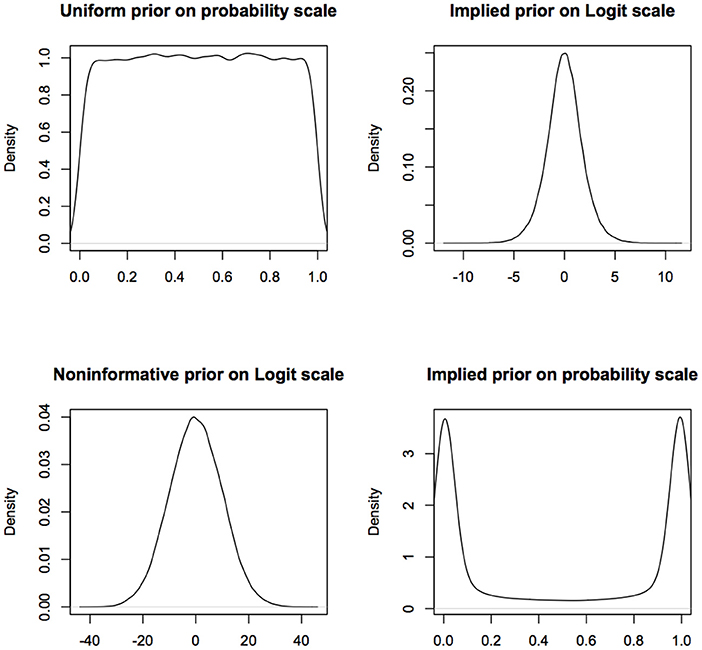
Figure 1. Non-informative prior on one scale is informative on a different scale. What is considered non-informative on the logit scale will be considered quite informative on the probability scale and what is considered non-informative on the probability scale will be considered informative on the logit scale. For computational convenience, the figures are density plots of the random numbers generated from the corresponding distributions, instead of using the analytic expressions.

This makes no sense because they are one-one transformations of each other; if we are ignorant about one, we should be equally ignorant about the other.

Fisher's criticism was potent enough that it needed addressing. Harold Jeffreys tried to construct priors that yield parameterization invariant conclusions. They are now known as Jeffreys priors. A full description of these priors and how to construct them is beyond the scope of this paper (See Press, 2003 or Ronneberg, 2017 for easily accessible details). However, it suffices to say that they are proportional to the determinant of the inverse of the expected Fisher information matrix.

Despite its theoretical properties, there are practical issues that hinder the use of Jeffrey's priors. For example, in order to construct them, one needs to know the likelihood function and the exact analytic expression for the expected Fisher information matrix. Because it is nearly impossible to write the likelihood function explicitly for hierarchical models, computing the expected Fisher information matrix is seldom possible for hierarchical models. This makes the specification of Jeffrey's prior for a given hierarchical model difficult.

Let us look at Jeffreys prior for a simple, non-hierarchical model where Y ~ Bernoulli(p). The Jeffreys prior for the probability of success p is the Beta(0.5, 05) distribution. The density function of this random variable is U-shaped that is highly concentrated near 0 and 1 with very small weight in the middle (see Figure 2). It looks similar to the distribution in the lower right hand panel. Even when Jeffreys prior can be computed, it will be difficult to sell it as an objective prior to the jurors or the senators on the committee.

FIGURE 2

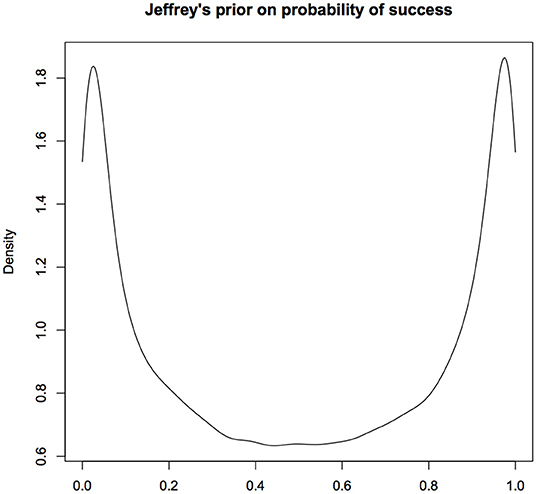
Figure 2. Jeffreys prior for probability of success in a Binomial experiment; This prior concentrates the probability mass near 0 and 1. It is difficult to justify this as a prior that would be considered non-informative. Multivariate extensions of Jeffreys priors can lead to inconsistent estimators and hence seldom used in practice. For computational convenience, the figures are density plots of the random numbers generated from the Uniform(0.5,0.5) distribution, instead of using the analytic expression.

Construction of Jeffreys and other objective priors for multi-parameter models poses substantial mathematical difficulties (Ronneberg, 2017). A commonly proposed solution is to put independent Jeffreys or other non-informative prior on each of the parameter separately. Why such prior knowledge of independence of the parameters be considered “non-informative” is unclear. Assuming two quantities are independent of each other is considered to be a very strong assumption in practice. The assumption of a priori independence between parameters is more a matter of convenience than a matter of principle and is not justifiable.

Press (2003, Chapter 5) provides an excellent review of various problems associated with the definitions and use of non-informative priors along with interesting historical notes. It is clear that non-informative priors are chosen more for their mathematical or computational convenience than for their representation of no information or because they “let the data speak.” Unfortunately, ecologists and practitioners tend to dismiss these criticisms; considering them to be of no practical relevance (e.g., Clark, 2005).

There are two prevalent notions, both false, about the non-informative Bayesian analysis. The first false notion is that there is no difference between non-informative Bayesian inference and likelihood-based inference and the second false notion is that the philosophical underpinnings of statistical inference are irrelevant to practice. Some researchers (e.g., Kery and Royle, 2016) even claim that Bayesian inference is “valid” for all sample sizes, but, unfortunately, without specifying the “validity” criterion. Of course, as the information in the sample increases, effects of the prior and consequences of lack of parameterization invariance become negligible. Although, caveat of large sample size is mathematically correct, whether or not the observed sample size is large depends on the complexity of the model and the strength of the prior (e.g., Dennis, 2004) and cannot be judged in practice. To illustrate the falsity of these notions for sample sizes observed in practice, we consider two important ecological problems: Population monitoring and population viability analysis. We show that, due to lack of invariance, analysis of the same data under the same statistical model can lead to substantially different conclusions under a non-informative Bayesian framework. This is disturbing because common sense dictates that same data analyzed using the same model should lead to the same scientific conclusions. The problem with the non-informative priors is that they do not “let the data speak”; contrary to what is commonly claimed, (absent large sample size) they bring in their own biases in the analysis. We do not suggest that likelihood analysis, which is parameterization invariant, is the only right way to do the data analysis in applied ecology. That debate is subtle and potentially unresolvable. Only goal of this paper is to show that implications of the lack of invariance of non-informative priors are of practical significance to wildlife managers.

2. Population Viability Analysis (PVA) for San Joaquin Kit Fox

Let us consider the San Joaquin kit fox data set originally analyzed by Dennis and Otten (2000). This kit fox population inhabits a study area of size 135 km² on the Naval Petroleum Reserves in California (NPRC). The abundance time-series for the years 1983–1995 was obtained to conduct an extensive population dynamics study as part of the NPRC Endangered Species and Cultural Resources Program. The annual abundance estimates were obtained from capture-recapture histories generated by trapping adult and yearling foxes each winter between 1983 and 1995. We refer the reader to Dennis and Otten (2000) for further details on these data and abundance estimation technique.

Dennis and Otten (2000) analyzed these data using the Ricker model. The deterministic version of the Ricker model can be written in two different but mathematically equivalent forms. It may be written in terms of the growth parameter a and density dependence parameter b as logN_t+1 − logN_t = a − bN_t where a > 0, b > 0 or in terms of growth parameter a and carrying capacity parameter K as $log{N}_{t+1}-log{N}_t=a\left(1-\frac{N_t}{K}\right)$ where a > 0, K > 0. We also know that K = a/b and b = a/K. It is reasonable to expect that the conclusions about the survival of the San Joaquin kit fox population would remain the same whether one uses the (a, b) formulation or the (a, K) formulation. In statistical jargon, we call this change in the form of the model “reparameterization” and we will use this term, instead of the term “different formulation,” in the rest of the paper. Following Dennis and Otten (2000), we use a stochastic version of the Ricker model where the parameter a, instead of being fixed, varies randomly from year to year. Furthermore, the abundance values are themselves an estimate of the true abundances and hence we consider the sampling variability in the model as well. The variances for the abundance estimates were nearly proportional to the abundance estimates and hence the Poisson sampling distribution makes reasonable sense. The full model can be written as a state-space model as follows. In the following, N_t denotes the true abundance, Y_t denotes the estimated abundance and X_t = logN_t.

We call the following form of the model the (a, b) parameterization.

• Process model: $X_{t+1}|X_t~Normal(X_t+a-b*exp(X_t),{\sigma }^2)$

• Observation model: Y_t|X_t ~ Poisson(exp(X_t))

One can write this model in an alternative form that we call the (a, K) parameterization.

• Process model: $X_{t+1}|X_t~Normal(X_t+a\left(1-\frac{exp(X_t)}{K}\right),{\sigma }^2)$ where K is the carrying capacity.

• Observation model: Y_t|X_t ~ Poisson(exp(X_t))

These two models are mathematically identical to each other. Our goal is to fit these models to the observed data and conduct population viability analysis using the population prediction intervals (PPIs) (Saether et al., 2000). To compute the one sided PPIs, that is usually of interest to managers, we predict the future values of the time series and connect the lower 10% values for each year to get a curve, as a function of time, indicating the lower envelope to the future population sizes. This lower envelope helps guide the management decisions. Common sense dictates that because the data are the same and the models are mathematically equivalent to each other, the PPIs computed under the two parameterizations should also be identical to each other.

We use Bayesian inference using non-informative priors to compute PPIs under these two forms. For Bayesian inference, we use the following non-informative priors for the parameters in the respective parameterization.

• Priors for the (a, b) parameterization: a ~ LN(0, 10), b ~ U(0, 1), σ² ~ LogNormal(0, 10)

• Priors for the (a, K) parameterization: a ~ LN(0, 10), K ~ Gamma(100, 100), σ² ~ LogNormal(0, 10)

These are some of the commonly used distributions for representing non-information on the appropriate ranges of the parameters (e.g., Kery and Schaub, 2011). Although note that there is no general agreement on what is a non-informative prior distribution. A reader who wants to use different non-informative priors can easily repeat the experiment by modifying the R code (see link in the data availability statement) appropriately. The qualitative conclusions will remain the same. For comparison, we use the data cloning algorithm (Lele et al., 2007, 2010) to compute the maximum likelihood estimators (MLE) based frequentist predictions to obtain PPIs under these two parameterizations. The analysis was conducted using the package “dclone” (Solymos, 2010; R Development Core Team, 2011), that is based on commonly used JAGS software (Plummer, 2003), within the R software. The data and the R program to conduct this analysis are available in the link provided in the data availability statement. Both Bayesian analysis and data cloning based maximum likelihood analysis are based on the Markov Chain Monte Carlo (MCMC) algorithms. Convergence diagnostics were based on the Gelman-Rubin Rhat statistics and the trace plots. For all cases, the Rhat statistics was very close to 1 and the trace plots showed good mixing of the chains (see link in the data availability statement). The resultant parameter estimates are given in the table below. To make the comparison easy to interpret, we report the estimates for (a, K, σ) under the two parameterizations.

Notice that (Table 1) the Bayesian parameter estimates for the two parameterizations, especially the estimates of the carrying capacity K, are quite a bit different. On the other hand, the data cloned maximum likelihood estimates (MLE) are nearly identical to each other under both parameterizations, as they should be. The small differences are due to the Monte Carlo error. In Figure 3, we show the PPIs obtained under the likelihood and the non-informative Bayesian approaches.

TABLE 1

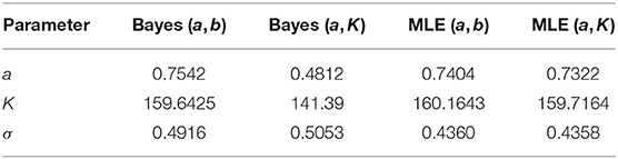
Table 1. Parameter estimates for the kit fox data using different parameterizations and non-informative priors and maximum likelihood.

FIGURE 3

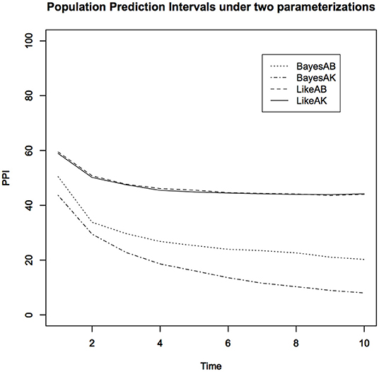
Figure 3. Lower 10% Population Prediction Intervals (PPI) for the kit fox data using non-informative Bayesian analysis under two different parameterizations and the maximum likelihood analysis. Notice that non-informative Bayesian analysis does not approximate the maximum likelihood analysis and depends on the specific parameterization.

One can make two important observations:

1. The PPIs obtained under the (a, b) parameterization and the PPIs obtained under the (a, K) parameterization, under purportedly non-informative priors, are quite different. Depending on which parameterization the researcher happens to use, the scientific conclusions could be quite different. For the non-informative Bayesian analysis, instead of the Gamma distribution, we also used a uniform distribution prior for the carrying capacity parameter. The results were not only different from these but also very sensitive to the choice of the upper bound of the uniform distribution. This is at least disturbing, if not totally unacceptable. As we said earlier, analyzing the same data with the same model should lead to the same conclusions. However, non-informative Bayesian analysis does not satisfy this common sense requirement.

2. The MLE based PPIs are quite different than the non-informative prior based PPI. Contrary to what is commonly claimed, the non-informative priors do not lead to inferences that are similar to the likelihood inferences.

3. Occupancy Models and Decline of Amphibians

One of the central tasks that applied ecologists are entrusted with is monitoring existing populations. These population monitoring data are the inputs to many further ecological analyses. We consider the following simple model that is commonly used in analyzing occupancy data with replicate visits (MacKenzie et al., 2002). We denote probability of occupancy by ψ and probability of detection, given that the site is occupied, by p. For simplicity (and, to emphasize that these results happen even for simple models), we assume that these do not depend on covariates. We assume that there are n sites and each site is visited k times. Other assumptions about close population and independence of the surveys are similar to the ones described in MacKenzie et al. (2002). In the following, Y_i indicates the true state of the ith location, occupied (1) or unoccupied (0). This is a latent, or unobservable, variable. Observations are denoted by O_ij. These are either 0 or 1, depending on the observed status of the location at the time of jth visit to the ith location. These can be different from the true state Y_i because of detection error. The replicate visit model can be written as follows.

• Hierarchy 1: Y_i ~ Bernoulli(ψ) for i = 1, 2, …, n

• Hierarchy 2: O_ij|Y_i = 1 ~ Bernoulli(p) where j = 1, 2, …, k

We assume that if Y_i = 0, then O_ij = 0 with probability 1 for j = 1, 2, …, k. That is, there are no false detections. This model can also be written in terms of logit parameters as follows:

• Hierarchy 1: $Y_i~Bernoulli(\frac{exp(\beta )}{1+exp(\beta )})$ for i = 1, 2, …, n where β = log(ψ/(1−ψ))

• Hierarchy 2: $O_{ij}|Y_i=1~Bernoulli(\frac{exp(\delta )}{1+exp(\delta )})$ for i = 1, 2, …, n where δ = log(p/(1−p))

The second parameterization is commonly used when there are covariates and the logit link is used to model the dependence of the occupancy and detection probabilities on the covariates. Notice that $p=\frac{exp(\delta )}{1+exp(\delta )}$ and $\psi =\frac{exp(\beta )}{1+exp(\beta )}$. If there are covariates that affect the occupancy probability, the familiar Logistic regression corresponds to $\psi (X_i)=\frac{exp({\beta }_0+{\beta }_1{X}_i)}{1+exp({\beta }_0+{\beta }_1{X}_i)}$.

We use the following non-informative priors for the two parameterizations.

• The (ψ, p) parameterization: ψ ~ Uniform(0, 1) and p ~ Uniform(0, 1)

• The (β, δ) parameterization: β ~ N(0, 1000) and δ ~ N(0, 1000)

These are commonly used non-informative priors on the respective scales (e.g., Kery and Schaub, 2011). One of the important goals of occupancy studies is to compute the probability that a site is, in fact, occupied when it is observed to be unoccupied on all visits. This is different than ψ. To compute this, we need to compute the probability that a site that is observed to be unoccupied is, in fact, occupied. We can compute it by using standard conditional probability arguments as: $P(Y_i=1|O_{ij}=0,j=1,2,..,k)=\frac{{(1-p)}^k\psi }{{(1-p)}^k\psi +(1-\psi )}$.

We first present a simulation study where we show the differences in the non-informative Bayesian inferences between the two parameterizations. The R program used to conduct these simulations is available in the link provided in the data availability statement. We present the simulation results for the case of 30 sites and two visits to each site. We consider three different combinations of probability of detection and probability of occupancy; both detection and occupancy small, occupancy large but detection small and occupancy small and detection large.

Table 2 shows that the Bayesian inferences about point estimates of the probability of occupancy and detection and more importantly about the probability that a site is, in fact, occupied when it is observed to be unoccupied on both visits (denoted by “occupancy” in the table for brevity) are dependent on the parameterization. This has significant practical implications: The total occupancy rate (defined explicitly in the next paragraph), that is often needed by the managers, depends on P(Y_i = 1|O_ij = 0, j = 1, 2, .., k), will be quite different depending on which parameterization is used. The biases observed here, although somewhat reduced, persisted as the sample size was increased to 50 and 100 but with only two visits per site. Notice also that variation under probability scale and logit scale are quite different. For more detailed simulations on the effect of prior distributions on the parameter estimation (but not the prediction) when covariates are involved, see Northrup and Gerber (2018) and comments that follow the paper.

TABLE 2

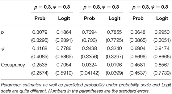
Table 2. Simulation results for n = 30 and k = 2.

How does this work out in real life situation? Let us reanalyze the data presented in MacKenzie et al. (2002). We consider a subset of the occupancy data for American Toad (Bufo americanus) where we only consider the first three visits. The data and the R program for this analysis are provided in the link provided in the data availability statement. As in the previous example, we conducted standard diagnostic tests such as the value of Gelman-Rubin statistics and trace plots to judge the convergence of the MCMC algorithm. In all case, we had excellent convergence. There are 27 sites that have at least three visits. Number of sites that were observed to be occupied at least once during the three visits was 10. Hence, the raw occupancy rate, the proportion of sites occupied at least once in three visits, was 0.37. We fit the constant occupancy and constant detection probability model using the two different parameterizations described above. We report, in Table 3, the Bayesian point estimates of: Probability of detection (p), probability of occupancy (ψ), probability of occupancy when the site was never observed to be occupied during the three visits, namely, P(Y_i = 1|O_ij = 0, j = 1, 2, .., k) under two different parameterizations. The total occupancy rate is computed by adding the number of sites that were observed to be occupied at least once during the surveys (these are the sites that are definitely occupied) to the probability of occupancy for those sites that were never observed to be occupied during the surveys (these sites might have been occupied but were not observed to have been occupied due to detection error), namely P(Y_i = 1|O_ij = 0, j = 1, 2, .., k) and dividing the number by the total number of sites. Total occupancy rate is often used to make management decisions.

TABLE 3

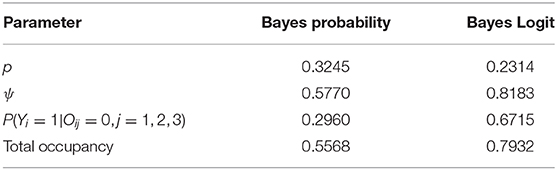
Table 3. Parameter estimates for the American Toad occupancy data using non-informative Bayesian under different parameterization.

The differences in the two analyses are striking. According to one analysis, we will declare an (observed to be) unoccupied site to have probability of being occupied as 0.296 where as the other analysis it is 0.672, more than double the first analysis. Given the data, after adjusting for detection error, we will declare the study area to have occupancy rate to be 0.56 under one analysis but under the other analysis, we will declare it to be 0.79. Both of these Bayesian estimates also differ from the ML estimate of 0.55 (This is slightly different than the one reported, 0.49, in MacKenzie et al., 2002 because, unlike the original analysis, we have considered a subset of sites that were visited exactly three times for ease of computation). The ML estimate is close to the Bayesian estimate with a flat prior on the probability scale but not to the one obtained by non-informative prior on the Logit scale.

In Figure 4, we show the posterior distributions for the total occupancy rate under the two parameterizations.

FIGURE 4

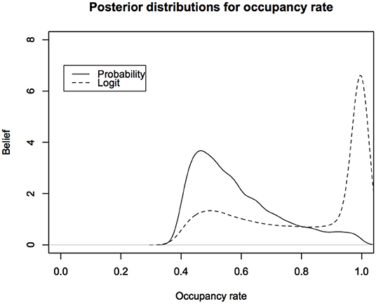
Figure 4. Posterior predictive distributions for the occupancy rates of American Toad under different parameterizations: The logit scale leads to a distribution that is highly skewed toward probability of occupancy close to 1. Probability of occupancy often depends on habitat covariates and is modeled with Logistic regression. This figure indicates that we might be biasing the inferences about probability of occupancy under the non-informative Bayesian analysis.

The difference between the two posterior distributions is shocking. Such posterior distributions form the basis for deciding the status of the species. It is obvious that the decisions based on these two posterior distributions are likely to be very different. Now imagine facing a lawyer in the court of law or a politician who is challenging the results of the wildlife manager who is testifying that the occupancy rates are too low (or, too high for invasive species). All they have to do, while still claiming to do a legitimate non-informative analysis, is use a parameterization that gives different results to raise the doubt in the minds of the jurors or the senators on the committee. This is not a desirable situation.

4. Unintended Consequences of Objective Priors

Scientific and statistical inference is not limited to inference about the parameters of the generating mechanism as it is formulated. Inference also extends to inference on functions of the parameters, including predictions. So far, we have studied in concrete terms the consequences of the lack of parameterization invariance in important ecological problems at commonly observed sample sizes, especially in wildlife management. These consequences, of course, vanish as the information in the data increases. Unfortunately, whether or not the observed sample size is large depends on the complexity of the model. In this section, we provide general arguments against subjective and objective priors in scientific inference in general.

Consequence 1: All subjective Bayesian inferences can be masqueraded as objective (flat prior) Bayesian inferences.

This result is simply a converse of Fisher's result that all flat priors on one scale are not flat on any other scale. Let Y be a random variable such that Y ~ f(.;θ). Let θ⊂Θ be continuous and Θ be a compact subset of the real line. Let π(θ) denote the prior distribution. A basic probability result on transformation (e.g., Casella and Berger, 2002) is the following: If θ ~ π(θ), then the probability density function of g(θ), a one-one, differentiable transformation of θ is given by $\pi (g^{-1}(\theta ))|\frac{d{g}^{-1}(\theta )}{d\theta }|$.

Thus, if θ has uniform distribution on Θ, any one-one, differentiable transformation of it has a density function that is proportional to $|\frac{d{g}^{-1}(\theta )}{d\theta }|$ which is not a uniform distribution. This is the basis of Fisher's criticism of the flat priors: What is “non-informative” on one scale is “informative” on any transformed scale.

The converse of the result, not noted in the literature to the best of our knowledge, is equally devastating. Suppose a researcher has a subjective prior in mind, say π(θ) that is not a uniform distribution on Θ. Let G(θ) denote the cumulative distribution function corresponding to this density. The researcher may have this particular prior in mind because he truly believes it but he realizes that he may face the criticism of being biased with an agenda to prove. To avoid the criticism, he can easily rewrite his model in terms of φ = G⁻¹(θ). This transformation is also known as the probability transform and is used to generate random numbers from univariate, continuous random variables (Gentle, 2004). It is well known that φ has a Uniform distribution on (0, 1). When presenting the results of his analysis, the researcher simply presents his model in terms of φ and a Uniform prior on (0, 1). Many Bayesian analysts would consider this as an “objective” Bayesian analysis that is not tainted by subjective priors and that it has “let the data speak.” This is patently a false statement: The researcher started with a subjective prior but was able to masquerade it as an “objective” analysis.

Consequence 2: Induced priors on functions of parameters are not flat, thus leading to cryptic biases in scientific inference.

Scientific inference is usually not limited to the natural parameters of the generating mechanism but may be based on functions of parameters. Often these functions of the natural parameters are really the parameters of scientific interest. For example, in the PVA example that we studied, the natural parameters of the Ricker model were (a, b) or (a, K). But the analysis was not limited to conducting inference about these parameters alone. We are interested in computing the probability of extinction or the time to extinction or the PPI (e.g., Dennis et al., 1991). These are usually functions of the natural parameters. Similarly for the occupancy model, the natural parameters are (ψ, p) but quantities of interest are predicted probability of occupancy when the site was never observed to be occupied. As we saw earlier, this is also a function of the natural parameters. When one specifies a prior distribution on the natural parameters, it induces a prior distribution on all transformations of the natural parameters including such functions of the parameters.

In PVA, one of the quantities of interest is the probability of (quasi)extinction, that is, the probability that the population will dip below a threshold. For the stochastic versions of the continuous time exponential growth models, Dennis et al. (1991) compute this explicitly. The basic model (for discrete time case) may be written as: $X_{t+1}|X_t~Normal(X_t+\mu ,{\sigma }^2)$. Let x_e be the log-threshold population size and x₀ be the current log-population. Let x_d = x₀ − x_e. The probability of (quasi)extinction is given by $\pi (x_d,\mu ,{\sigma }^2)=exp(-2\mu x_d/{\sigma }^2)$ for μ > 0. If μ < 0, the population goes to extinction with certainty and hence that case is not of interest. In Figure 6, we show the priors induced on this quantity under different non-informative priors on μ and σ² (without changing the parameterization). The solid curve corresponds to using μ ~ logNormal(0, 10) and σ ~ logNormal(0, 10) and the dotted curve corresponds to using μ ~ Uniform(0, 10) and σ ~ Uniform(0, 10).

Let us look at the induced prior distribution for $P(Y_i=1|O_{ij}=0,j=1,2,..,k)=\frac{{(1-p)}^k\psi }{{(1-p)}^k\psi +(1-\psi )}$, the predicted occupancy, under different non-informative priors of p and ψ for k = 2. The solid curve in Figure 5 corresponds to the induced prior on the predictive occupancy using ψ ~ Uniform(0, 1) and p ~ Uniform(0, 1) and the dotted curve corresponds to using non-informative prior commonly used on the (β, δ) scale as described previously in the discussion of the occupancy problem, namely, β ~ Normal(0, 10) and δ ~ Normal(0, 10).

FIGURE 5

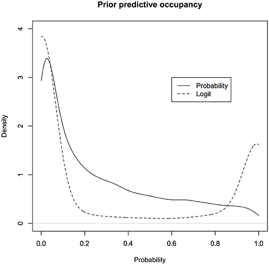
Figure 5. Induced priors on the quasi extinction probability: Different non-informative priors on the parameters of a stochastic Exponential growth model lead to different induced priors on the probability of quasi-extinction. We are biasing the result even before any data are conducted. The induced prior on the probability of quasi-extinction, the parameter of interest, is not uniform. One induced prior (red) is implicitly assuming that probability of extinction is highly likely to be zero whereas another induced prior (blue) implicitly assumes the probability of extinction is mostly between 0 to 0.2 or 0.8 to 1 but not much in between.

FIGURE 6

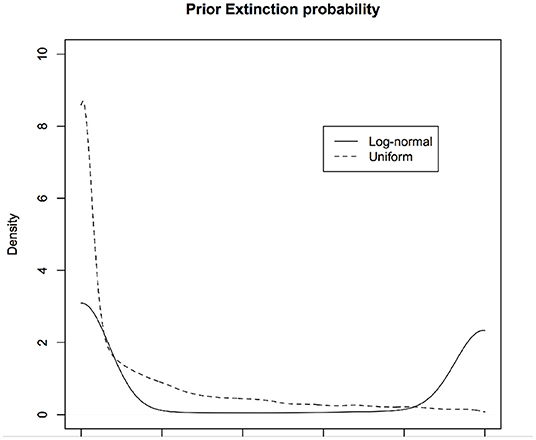
Figure 6. Induced priors on the occupancy probability: Different non-informative priors induce different priors on the parameter of interest, namely, probability that a site is occupied given that we have not observed it to be occupied while surveying due to detection error. We are biasing the results of the survey even before conducting the survey. One induced prior (black) is implicitly assuming that probability of occupancy is more likely to be zero whereas another induced prior (red) implicitly assumes the probability of occupancy is near 0 or 1 but not much in between.

It is clear that different versions of the non-informative priors on the natural parameters induce different priors (and, hence biases) on the induced parameters that are of scientific interest. In Lele (2004) and Lele and Allen (2006), it was argued that even if one can elicit priors from the experts on the natural parameters, expert may not be aware of, and in fact, may not even agree with the prior distributions induced by his own priors on the natural parameters. In a recent paper, Seaman et al. (2012) point out the same issues but in the context of flat priors, extending Fisher's criticism of the flat priors.

There is a hidden danger of using flat priors uncritically. Unwittingly the researcher might be biasing the conclusion about the interesting functions of the parameters while falsely claiming the mantle of “objectivity.” Even when we have flat priors on the natural parameters, the induced priors on the quantities of inferential interest are extremely likely to be biased to one conclusion or the other.

Consequence 3: The assumption of independent parameters, although convenient for MCMC calculations, creates unrealistic priors.

Most ecological models involve multiple parameters with complex parameter spaces. Because of the interdependencies between these parameters, the valid parameter values are dependent on each other. It is usually quite difficult to specify flat priors or almost flat priors as in priors with large variability on such non-trivial parameter spaces. Even Jeffreys priors (e.g., Ronneberg, 2017) that address Fisher's objection and are invariant to parameterization, or Bernardo's reference priors (e.g., Ronneberg, 2017) are extremely difficult to construct for multiparameter situations. In practice, most of the Bayesian analysis for multiparameter models is conducted with priors that assume that parameters are a priori independent. For example, in simple Capture-Recapture models, it is often assumed (e.g., Parent and Rivot, 2013) that probability of recapture and population size are independent of each other. Similarly in regression analysis, it is assumed that the regression parameters are independent of the each other a priori. In fact, as is clear from any analysis of Capture-Recapture experiments that the parameters are intricately related to each other. The assumption of prior independence of parameters is seldom justified but is taken as a convenient assumption. Questions one must ask are: What are the consequences on the distribution of the functions of parameters that are of real interest? What effect would this have if we reparameterize the model where new parameters are functions of the original parameters? For example, if we assume (a, b) are independent of each other, it is clear that (a, K) are bound to be correlated parameters because K, the carrying capacity, is a function of both a, growth parameter and b, the density dependence parameter. Is this correlation sensible a priori?

Ecologists are justifiably skeptical of the assumption that the data are independent of each other and are well aware of the consequences of such assumption; the famous pseudo replication problem in ecology (Hurlbert, 1984). However, they seem to accept, somewhat uncritically, the assumption of a priori independence between the parameters. Computational convenience should not be the driving force behind choosing prior distributions. Prior distributions have consequences; sometimes they are intended but most of the times they are unintended and not understood explicitly.

Consequence 4: Bayesian prediction intervals may not have correct coverage

Management decisions are based not only on the parameter estimates but also, and perhaps more importantly, on prediction of future events. In an important recent paper, Shen et al. (2018) consider the problem of prediction and predictive densities from the Classical and Bayesian perspective. They define a predictive density in a general form as: f^P(y) = ∫f(y; θ)dQ(θ). They show that such predictive density will lead to correct predictive coverage provided Q(θ) is a valid confidence distribution that has correct frequentist coverage properties. As a consequence, the Bayesian predictive density that uses posterior distribution as Q(θ), will lead to valid predictive coverage only if the posterior distribution has correct frequentist properties. Unfortunately, posterior distributions do not always have, in fact seldom have, correct frequentist coverage properties unless the information in the data is substantial. Of course, in that case, there remains no difference between a Bayesian and a frequentist inference.

Whether information in the data is substantial or not is not a simple function of the sample size; it also depends on the complexity of the model. The more complex the model is, the larger is the sample size required (e.g., Dennis, 2004). As a consequence, the objective, flat prior based analyses may not even lead to predictions that are valid. Why should we expect them to lead to management decisions that are sensible in practice?

Consequence 5: Reparameterization to facilitate MCMC convergence may influence scientific inference.

Markov Chain Monte Carlo algorithms have made it feasible to analyze highly complex, hierarchical models. One of the major difficulties in the application of the MCMC algorithms is the convergence of the underlying Markov chain to stationarity. When the parameters in the model are highly correlated (also, termed weakly estimable) or if the parameters are non-identifiable or non-estimable (See Ponciano et al., 2012; Campbell and Lele, 2014), it is difficult to obtain convergence and good mixing of the MCMC chains.

To alleviate this problem, one needs to reparameterize the model so that the parameters are orthogonal or weakly correlated with each other. Such reparameterization of the model will have no consequences if the inferences are based on the likelihood function which is invariant to such reparameterization but, as shown above, can have serious consequences for a non-informative Bayesian inference.

As an aside, such orthogonalization of the parameters is feasible only if the parameters are identifiable. Diagnostics for non-estimability and non-identifiability of the parameters is automatic under the data cloning based likelihood estimation (Lele et al., 2010; Ponciano et al., 2012; Campbell and Lele, 2014), however such diagnostics is not possible under the Bayesian approach (Lele, 2010).

5. Discussion

Using different parameterizations of a statistical model depending on the purpose of the analysis is not uncommon. For example, in survival analysis the exponential distribution is written using the hazard function or the mean survival function depending on the goal of the study. They are simply reciprocals of each other. Similarly Gamma distribution is often written in terms of rate and shape parameter or in terms of mean and variance that is suitable for regression models. Beta regression is presented in two different forms: regression models for the two shape parameters or a regression model for the mean keeping variance parameter constant (Ferrari and Cribari-Neto, 2004). All these situations present a problem for flat and other non-informative priors because same data and same model can lead to different conclusions depending on which parameterization is used. One can possibly construct similar examples in the Mark-Capture-Recapture methods where different parameterizations are commonly used.

Indeed, as the sample size increases, effect of the prior diminishes and Bayesian and likelihood inferences become similar. However, in practice, hierarchical models are fairly complex and involve substantially more parameters than in the models considered in this paper. Dennis (2004) illustrates that as number of parameters increases, effects of the choice of a prior linger even for large samples.

Hierarchical models in ecology tend to be complex and can easily lead to non-identifiable parameters (Lele et al., 2010; Ponciano et al., 2012; Campbell and Lele, 2014). If there are non-identifiable parameters, effect of the prior never vanishes. Owhadi et al. (2015) explore effect of the priors on Bayesian inferences in a mathematically rigorous fashion and conclude that the Bayesian inference is very brittle. Hence, the results presented here are likely to be far more common in practice than may be imagined.

To summarize, we have shown that non-informative priors neither “let the data speak” nor does the analysis based on them correspond, even roughly, to likelihood analysis for the sample sizes feasible in ecological studies. Non-informative priors add their own cryptic biases to the scientific conclusions. Just because the terms objective priors, non-informative priors or objective Bayesian analysis are used, it does not mean that the analyses are not subjective. A truly subjective prior based on expert opinion is, perhaps, preferable to the non-informative priors because in the former case the subjectivity is clear and well quantified, and, may even be justified, whereas in the latter the subjectivity is hidden and not quantified.

Hierarchical models in themselves are extremely useful to model complex ecological phenomena. The many successes of the so called “Bayesian” approach are actually attributable to sensible uses of hierarchical models for pooling information, e.g across different studies or resolutions. These success stories have nothing to do with the use of the Bayesian philosophy or use of priors.

Many applied ecologists are using the non-informative Bayesian approach as a panacea to deal with hierarchical models, erroneously believing that they are presenting objective, unbiased results and that there are no alternative approaches. Hierarchical models can be and are analyzed using the likelihood and frequentist methods. Given the complexity of these models, the number of parameters involved and the different ways the same model potentially can be formulated; the resultant analysis, because of the lack of invariance to parameterization, may have unstated and unqualified biases. Hence it may be easily challenged in the legislature and in the court of law.

Data Availability Statement

This R code and data are available at: https://github.com/jmponciano/LELE_NoninformativeBayes.

Author Contributions

SL conceived of the project, conducted the analysis and wrote the paper.

Funding

This work was partially supported by a grant from National Science Engineering Research Council of Canada to SL.

Conflict of Interest

The author declares that the research was conducted in the absence of any commercial or financial relationships that could be construed as a potential conflict of interest.

Acknowledgments

This work was initiated while the author was visiting the Center for Biodiversity Dynamics, NTNU, Norway and the Department of Biology, Sun Yat Sen University, Guangzhou in 2014. Two anonymous referees along with H. Beyer, B. Dennis, C. McCulloch, J. Ponciano, P. Solymos and especially M. Taper provided many useful comments that have improved the manuscript significantly. B. Dennis provided the kit fox data. This paper is an extended version of an arXiv paper (Lele, 2014).

References

Bolker, B. M. (2008). Ecological Models and Data in R. Princeton, NJ: Princeton University Press.

Google Scholar

Campbell, D., and Lele, S. R. (2014). An ANOVA test for parameter estimability using data cloning with application to statistical inference for dynamic systems. Comput. Stat. Data Anal. 70, 257–267. doi: 10.1016/j.csda.2013.09.013

CrossRef Full Text | Google Scholar

Casella, G., and Berger, R. L. (2002). Statistical Inference, Vol. 2. Pacific Grove, CA: Duxbury Press.

Google Scholar

Clark, J. S. (2005). Why environmental scientists are becoming Bayesians. Ecol. Lett. 8, 2–14. doi: 10.1111/j.1461-0248.2004.00702.x

CrossRef Full Text | Google Scholar

De Valpine, P. (2009). Shared challenges and common ground for Bayesian and classical analysis of hierarchical statistical models. Ecol. Appl. 19, 584–588. doi: 10.1890/08-0562.1

PubMed Abstract | CrossRef Full Text | Google Scholar

Dennis, B. (1996). Discussion: should ecologists become Bayesians? Ecol. Appl. 6, 1095–1103. doi: 10.2307/2269594

CrossRef Full Text | Google Scholar

Dennis, B. (2004). “Statistics and the scientific method in ecology,” in The Nature of Scientific Evidence, eds M. L. Taper and S. R. Lele (Chicago, IL: University of Chicago Press), 327–378.

Google Scholar

Dennis, B., Munholland, P. L., and Scott, J. M. (1991). Estimation of growth and extinction parameters for endangered species. Ecol. Monogr. 61, 115–143. doi: 10.2307/1943004

CrossRef Full Text | Google Scholar

Dennis, B., and Otten, M. R. (2000). Joint effects of density dependence and rainfall on abundance of San Joaquin kit fox. J. Wildlife Manage. 64, 388–400. doi: 10.2307/3803237

CrossRef Full Text | Google Scholar

Efron, B. (1986). Why isn't everyone a Bayesian? Am. Stat. 40, 1–5. doi: 10.1080/00031305.1986.10475342

CrossRef Full Text | Google Scholar

Ferrari, S. L. P., and Cribari-Neto, F. (2004). Beta regression for modelling rates and proportions. J. Appl. Stat. 31, 799–815. doi: 10.1080/0266476042000214501

CrossRef Full Text | Google Scholar

Fisher, R. A. (1930). Inverse probability. Math. Proc. Cambridge Philos. Soc. 26, 528–535. doi: 10.1017/S0305004100016297

CrossRef Full Text | Google Scholar

Gelman, A. (2006). Prior distributions for variance parameters in hierarchical models (comment on article by Browne and Draper). Bayesian Anal. 1, 515–534. doi: 10.1214/06-BA117A

CrossRef Full Text | Google Scholar

Gentle, J. E. (2004). Random Number Generation and Monte Carlo Methods. New York, NY: Springer.

Google Scholar

Hurlbert, S. H. (1984). Pseudo-replication and the design of ecological field experiments. Ecol. Monogr. 54, 187–211. doi: 10.2307/1942661

CrossRef Full Text | Google Scholar

Kery, M., and Royle, A. (2016). Applied Hierarchical Modelling in Ecology: Analysis of Distribution, Abundance and Species Richness in R and BUGS. New York, NY: Elsevier.

Google Scholar

Kery, M., and Schaub, M. (2011). Bayesian Population Analysis Using WinBUGS: A Hierarchical Perspective. New York, NY: Academic Press.

Google Scholar

King, R., Morgan, B., Gimenez, O., and Brooks, S. (2009). Bayesian Analysis for Population Ecology. Boca Raton, FL: CRC Press.

Google Scholar

Lele, S. R. (2004). “Elicit data, not prior: on using expert opinion in ecological studies,” inn The Nature of Scientific Evidence, eds M. L. Taper and S. R. Lele (Chicago, IL: University of Chicago Press), 410–436.

Google Scholar

Lele, S. R. (2010). Model complexity and information in the data should match: could it be a house built on sand? Ecology 91, 3493–3496. doi: 10.1890/10-0099.1

CrossRef Full Text | Google Scholar

Lele, S. R. (2014). Is non-informative Bayesian analysis appropriate for wildlife management: survival of San Joaquin Kit fox and declines in amphibian populations. arXiv:1502.00483.

Google Scholar

Lele, S. R., and Allen, K. L. (2006). On using expert opinion in ecological analyses: a frequentist approach. Environmetrics 17, 683–704. doi: 10.1002/env.786

CrossRef Full Text | Google Scholar

Lele, S. R., and Dennis, B. (2009). Bayesian methods for hierarchical models: are ecologists making a Faustian bargain. Ecol. Appl. 19, 581–584. doi: 10.1890/08-0549.1

PubMed Abstract | CrossRef Full Text | Google Scholar

Lele, S. R., Dennis, B., and Lutscher, F. (2007). Data cloning: easy maximum likelihood estimation for complex ecological models using Bayesian Markov chain Monte Carlo methods. Ecol. Lett. 10, 551–563. doi: 10.1111/j.1461-0248.2007.01047.x

PubMed Abstract | CrossRef Full Text | Google Scholar

Lele, S. R., Nadeem, K., and Schmuland, B. (2010). Estimability and likelihood inference for generalized linear mixed models using data cloning. J. Am. Stat. Assoc. 105, 1617–1625. doi: 10.1198/jasa.2010.tm09757

CrossRef Full Text | Google Scholar

Link, W. A. (2013). A cautionary note on the discrete uniform prior for the binomial N. Ecology 94, 2173–2179. doi: 10.1890/13-0176.1

PubMed Abstract | CrossRef Full Text | Google Scholar

MacKenzie, D. I., Nichols, J. D., Lachman, G. B., Droege, S., Andrew Royle, J., and Langtimm, C. A. (2002). Estimating site occupancy rates when detection probabilities are less than one. Ecology 83, 2248–2255. doi: 10.1890/0012-9658(2002)0832248:ESORWD2.0.CO;2

CrossRef Full Text | Google Scholar

Natarajan, R., and McCulloch, C. E. (1998). Gibbs sampling with diffuse priors: a valid approach to data driven inference? J. Comput. Graph. Stat. 7, 267–277. doi: 10.1080/10618600.1998.10474776

CrossRef Full Text | Google Scholar

Northrup, J. M., and Gerber, B. D. (2018). A comment on priors for Bayesian occupancy models. PLoS ONE 13:e0192819. doi: 10.1890/0012-9658(2002)083[2248:ESORWD]2.0.CO;2

PubMed Abstract | CrossRef Full Text | Google Scholar

Owhadi, H., Scovel, C., and Sullivan, T. (2015). Brittleness of Bayesian inference under finite information in a continuous world. Electr. J. Stat. 9, 1–79. doi: 10.1214/15-EJS989

CrossRef Full Text | Google Scholar

Parent, E., and Rivot, E. (2013). Introduction to Hierarchical Bayesian Modelling of Ecological Data. London: Chapman and Hall/CRC.

Google Scholar

Plummer, M. (2003). “JAGS: a program for analysis of Bayesian graphical models using Gibbs sampling,” in Proceedings of the 3rd International Workshop on Distributed Statistical Computing, 10.

Google Scholar

Ponciano, J. M., Burleigh, J. G., Braun, E. L., and Taper, M. L. (2012). Assessing parameter identifiability in phylogenetic models using data cloning. Syst. Biol. 61, 955–972. doi: 10.1093/sysbio/sys055

PubMed Abstract | CrossRef Full Text | Google Scholar

Press, S. J. (2003). Subjective and Objective Bayesian Statistics: Principles, Models and Applications, 2nd Edn. New York, NY: Wiley Interscience.

Google Scholar

R Development Core Team (2011). R: A Language and Environment for Statistical Computing. Vienna: R Foundation for Statistical Computing.

PubMed Abstract | Google Scholar

Rannala, B., Zhu, T., and Yang, Z. (2012). Tail paradox, partial identifiabilty and influential priors in Bayesian branch length inference. Mol. Biol. Evol. 29, 325–335. doi: 10.1093/molbev/msr210

PubMed Abstract | CrossRef Full Text | Google Scholar

Ronneberg, L. T. S. (2017). Fiducial and objective inference: history, theory and comparisons (Master's thesis). Department of Mathematics, University of Oslo, Oslo, Norway.

Google Scholar

Saether, B. E., Engen, S., Lande, R., Arcese, P., and Smith, J. N. (2000). Estimating the time to extinction in an island population of song sparrows. Proc. R. Soc. B Biol. Sci. 267:621. doi: 10.1098/rspb.2000.1047

PubMed Abstract | CrossRef Full Text | Google Scholar

Seaman, J. W. III., Seaman, J. W. Jr., and Stamey, J. D. (2012). Hidden dangers of specifying non-informative priors. Am. Stat. 66, 77–84. doi: 10.1080/00031305.2012.695938

CrossRef Full Text | Google Scholar

Shen, J., Liu, R. L., and Xie, M. (2018). Prediction with confidence? A general framework for predictive inference. J. Stat. Plan. Inference 195, 126–140. doi: 10.1016/j.jspi.2017.09.012

CrossRef Full Text | Google Scholar

Solymos, P. (2010). dclone: data cloning in R. R J. 2, 29–37. doi: 10.32614/RJ-2010-011

CrossRef Full Text | Google Scholar