Modeling the distribution of invasive species (Ambrosia spp.) using regression kriging and Maxent

Introduction

Invasion by non-native species through human activity is a major threat to biodiversity (Essl et al., 2020). International trade and tourism are direct causes of the rapid spread of non-native species (Fuller et al., 1984; Mills et al., 1994; Rejmánek and Randall, 1994). Although these invasive species are not dominant in their native environment, they often exhibit important traits, such as high growth rate and strong survivability, which can increase their population size, and assist in outcompeting native species in new habitats (Hinz and Schwarzlaender, 2004; Vilà et al., 2011). Moreover, persistent seeds play an important role in increasing the genetic diversity of invasive populations and increasing their adaptability to environmental changes (Gioria et al., 2012; Gioria and Pyšek, 2016). Additionally, invasion of non-native populations can change the genetic structure of native communities because of genetic interactions between the two populations (Prentis et al., 2008; Chun et al., 2009). Various species are translocated from their original places to new habitats by planned or unplanned human activities. Such translocated non-native species can negatively affect the native biodiversity and ecosystem (Mayfield et al., 2021). This negative impact is not only restricted to the ecosystem but also extends to the economy, society, and public health (Pimentel et al., 2005; Vilà et al., 2011; Warziniack et al., 2021).

The control of non-native species invasions is becoming increasingly important. The adverse effects of invasive species are well-recognized by the Korean government, and efforts to mitigate these negative effects have been underway since decades (Ministry of the Environment, 2019). In addition to identifying the habitat preferences of the target species (Kim et al., 2013; Lee et al., 2013; Hong et al., 2015), it is important to develop models that can accurately estimate the current spatial distribution and any distribution changes, to effectively control invasive species.

Species distribution models (SDMs) can model the relationship between occurrence (presence only or presence/absence) data and environmental factors to map the estimated spatial distribution. SDMs have been used to estimate the habitat suitability of non-native species and identify their potential distribution patterns (Smolik et al., 2010; Farashi and Najafabadi, 2015; Lee et al., 2016; Park et al., 2017; Früh et al., 2018; Ng et al., 2018). Predicting the potential distribution is important for the long-term management of non-native species. However, current distribution information of the target species is also critical for species management. In the most problematic cases, non-native species have been introduced recently (decades or years) and their habitats are currently expanding. Even in habitable regions, non-native species may not reach the maximum predicted distribution because of dispersal restrictions (not yet settled) or eradication campaigns (removed after settlement). Hence, we can assume that there is a large deviation between the potential and current (actual) distributions of these species. Potential distribution estimations provide basic information on habitat preference or suitability. Nevertheless, they do not always provide satisfactory information for the quantitative prediction of the current distribution and ongoing changes. Moreover, the lack of prediction accuracy hinders the accurate evaluation of the effect of invasive species removal. Invasive species are non-native species that may cause harm to the environment and have high adaptability and dispersal potential. The spatial distribution of invasive species is highly variable. For these reasons, it is difficult but important to predict the current distribution of invasive species. In contrast to previous studies on the potential distribution of invasive species (Ward, 2007; Lee et al., 2016; Park et al., 2017; Früh et al., 2018; Ng et al., 2018), studies on current distribution have rarely been conducted. Gormley et al. (2011) modeled the potential and current distributions of the invasive sambar deer using Maxent and occupancy models, respectively. Remote sensing (RS) is a useful and promising tool for identifying the current distribution of invasive plant species (Elkind et al., 2019; Dai et al., 2020). However, to utilize RS, the target species needs to be distinguished from other species based on the spectral characteristics of images, which acts as a constraint.

Various types of models have been used for SDMs. Species distribution can be estimated using statistical methods, such as the generalized linear model (GLM). More recently, various machine-learning methods, including the classification and regression tree (Breiman et al., 1984) and maximum entropy (Maxent) (Phillips et al., 2006) models have been applied to species distribution studies. Machine learning models have demonstrated an excellent ability to predict species distributions, effectively modeling the relationships between environmental factors and species occurrence. However, few models consider spatial autocorrelations or data proximity. Studies on invasive species distributions using these non-spatial models have evaluated habitat suitability and estimated the potential habitat of the target species (Park et al., 2015, 2017; Lee et al., 2016; Früh et al., 2018; Ng et al., 2018). Spatial models, such as regression-kriging (RK) (Hengl et al., 2009), which can consider spatial autocorrelation of occurrence data, have rarely been applied to model the distribution of invasive species.

Ambrosia trifida and Ambrosia artemisiifolia are annual herbs native to North America that have been accidentally introduced in several countries. These species readily colonize disturbed areas by producing a large number of seeds. In Korea, A. artemisiifolia was introduced during the Korean War, but it was reported first in 1968; presently, it is distributed evenly throughout the country (Kim, 2017). Additionally, A. artemisiifolia thrives on roadsides as well as in farmlands. Similarly, A. trifida was considered to be introduced along with livestock feed or US military supplies in north of Gyeonggi-do in the 1970s (Kil et al., 2004). A. trifida can reach a maximum height of 400 cm and behave as a dominant species throughout the entire growing season. Therefore, it can significantly decrease the native plant diversity and serves as a problematic species by decreasing the yield of cultivated agricultural crops (Kil et al., 2004). A large colony of A. trifida is frequently found on riversides and this species mainly spreads through flowing water. Contrastingly, A. artemisiifolia is more frequently found on the roadside and in drier soil. These two Ambrosia species produce highly allergenic pollen and can induce allergic rhinitis, fever, or dermatitis. Therefore, both species are designated as harmful invasive plants by the Ministry of the Environment of the Republic of Korea in 1999.

The aims of this study were to (1) analyze the environmental factors affecting the distribution of A. artemisiifolia and A. trifida, which are designated invasive species that are highly likely to cause ecosystem disturbances, (2) estimate the distribution of these species using the Maxent and RK models, and (3) evaluate the current distribution prediction performance of the models.

Materials and methods

Study area

This research was conducted in an inland area (excluding islands) of the Seoul metropolitan region, including Incheon and Gyeonggi-do. The area has the highest population density in South Korea and it is heavily urbanized. Incheon Port and Pyeongtaek Port are in the western section, where there are international logistics distribution centers. To the east, there are mountainous and high-altitude areas. To the north and south are low-altitude flatlands. However, the northern borders are strictly blocked for all movement. To the south is a high-density road network with heavy traffic connecting to other areas. In this region, many non-native species may potentially disperse through the road network. As the Hangang River mouth is in the study zone, non-native species can disperse with the river as well. Thus, it is important to manage non-native species in this area. The regional climate of the study area is temperate and the average annual temperature and precipitation are 12.5°C and ca. 1,400 mm, respectively. The regional population was 25,713,241 in 2018. Over several decades, the farmland and forests in the area have steadily declined due to the rapid urban expansion.

Data

Non-native species selection and data collection

A nationwide non-native species survey was conducted from 2015 to 2018 (National Institute of Ecology, 2019). In the study area, species data were collected in 2018 (from March to October). All species listed in the national non-native species database (Ministry of the Environment, 2019) were surveyed. Surveyors and taxonomy experts detected all non-native species communities and listed the species with the coordinates of their positions using a global positioning system receiver. The survey points were selected based on the investigator’s knowledge and field conditions. No predefined sampling design was applied. Thus, accessibility could have influenced the selection of the survey points. Therefore, the density and distribution of the survey points were irregular. The analysis was performed using a 100 × 100 m cell grid. Notably, the resolution was not based on the scale used in the field survey. The size of the field survey site was determined by the size of the invasive species community, rather than the predefined grid. The resolution scale aligned with the spatial resolution of the land cover (LC) data used in this study. The survey point coordinates were re-designated to the center of the cell coordinates. If there was more than one survey point in a single cell, then the species was listed with a single coordinate (the cell center). Based on these criteria, the total number of survey points was 1,478. At each survey point, the surveyor recorded all the species present in the community. Hence, the species data were regarded as presence/absence (P/A) data.

The Korean government has a designated invasive alien species (IAS) list. A species of the IAS list is a non-native species that heavily disturbs ecosystems or is likely to do so. As of 2022, 16 plant species have been listed. A. artemisiifolia L. var. elator and A. trifida L. var. trifida have been on the IAS list since 1999, when the IAS designation system was initiated. Both species are annual and ruderal species. They especially flourish in sunny environments but are not restricted to a specific environment (Smolik et al., 2010; Lee et al., 2016; Park et al., 2017; Ministry of the Environment and National Institute of Ecology, 2018). Both species share similar ecological traits, and their distributions partially overlap in the study area. A. artemisiifolia and A. trifida were detected at 239 (16%) and 716 (48.4%) survey points, respectively (Figure 1). Both species occurred in the same community in 106 cells. Each species had unique regional distribution characteristics. A. artemisiifolia is widely distributed in the southeast, whereas A. trifida is widely distributed in the northwest. A. artemisiifolia has a limited regional distribution, whereas A. trifida is widely distributed across all regions. Both local governments and conservationists have recognized these species as major harmful species and have conducted eradication activities over the past decades. Nevertheless, both species persist throughout the study area.

FIGURE 1

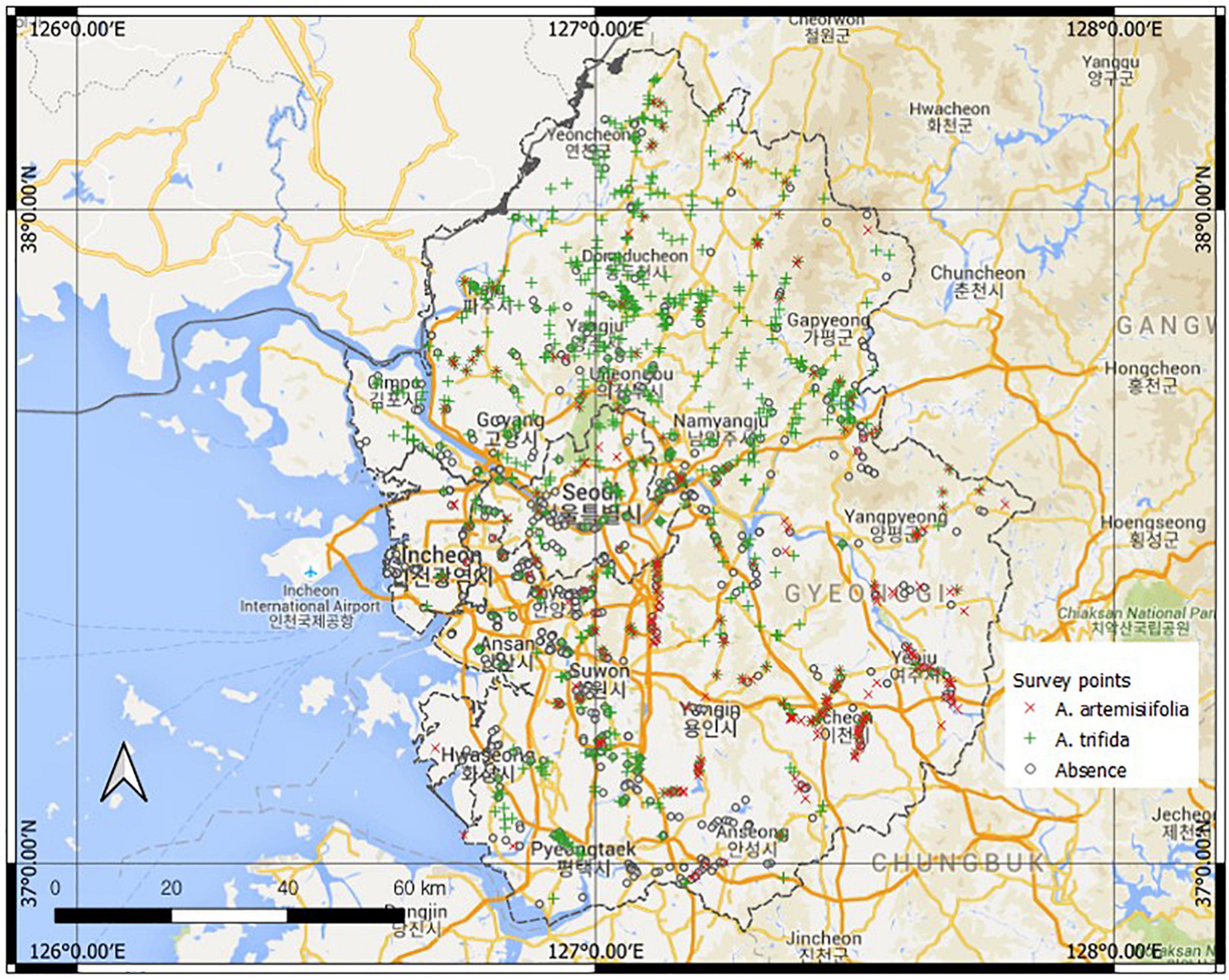
Figure 1. Study area (Google Maps, 2021) with field survey points.

Environmental data

Topographic data, LC data, and climate data were used as covariates of SDMs. ALOS World 3D 30-m mesh (AW3D30) v. 3.2¹ DEM (Tadono et al., 2016) was used to calculate the slope and aspect. We used fractional LC data provided by the Copernicus Global Land Service (CGLS) with a 100 m spatial resolution (Buchhorn et al., 2020). The fractional LC data provides more comprehensive information than the LC data with a single type. The data provide fractional information (0-100%) for each LC type present in each cell. The 2018 LC map was used. The CGLS LC data comprise ten LC classes. We used eight classes (tree, scrub, cropland, grassland, bare oil, built-up area, seasonal water, and permanent water), because these potentially influence Ambrosia spp. distributions. The climate data were obtained from WorldClim 30 v. 2.1.² Three uncorrelated climate factors, which are important for the target species (influencing the physiological characteristics and life history traits), were selected and used for modeling. The climate factors included the warmest quarter (Bio18), mean temperature of the warmest quarter (Bio10), and mean solar radiation between June and August. All data with the geographical coordinates were projected onto the projected coordinate system (Transverse Mercator Coordinate System; EPSG: 5179).

Predictive model

Generalized linear model

Generalized linear model logistic regression was used to model the relationship between species occurrence (P/A) data and environmental covariates. The following equation predicts the expected occurrence probability of Ambrosia spp. using the GLM.

$\text{Y}\left(\mathbf{P}\right)=\mathrm{\mu }=g^{-1}\left(\mathbf{\text{q}}\cdot \mathbf{\beta }\right)(1)$

where Y(P) is the expected probability of occurrence (P∈[0,1]), q is the environmental predictor, β is the coefficient of the linear model, and g is the link function. A logit link function was used. A full GLM model was constructed using all 15 environmental covariates (Table 1). Among the covariates, regression predictors were determined using stepwise selection based on the Akaike information criterion (AIC).

TABLE 1

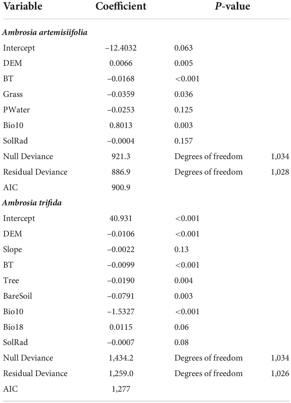
Table 1. Generalized linear model (GLM) results with the binomial error structure and logit link function.

The GLM models the occurrence (P/A) data variation in two terms: (a) variations that can be modeled (deterministic part; m) and (b) residual variation that cannot be modeled (error part; e). The probability of occurrence at site s can be expressed as:

$\text{Y}\left(s\right)=m\left(s\right)+e\left(s\right)(2)$

The deterministic (trend) part may be constant, but usually changes as a function of the covariates. Therefore, the probability of occurrence at a new location (s₀) can be predicted as follows:

$m\left(s_0\right)=\sum _{j=0}^p{\mathrm{\beta }}_j\cdot q_i\left(s_0\right)(3)$

where β_j is the regression model coefficient, q_i is the selected covariate (predictor), and p is the number of covariates.

The GLM can yield large residual variations, especially when the covariates only partially account for the dependent variable. This can also occur when the observations or measurements are dependent, which undermines the GLM assumptions. The spatial distribution modeling of IAS must address twofold challenges. Most IASs are generalists and not heavily restricted by specific environmental conditions. Therefore, it is often difficult to find a covariate with a sufficiently strong explanatory power to predict the IAS distribution. The distribution of the IAS can be limited by geographic constraints or dispersal efficiency. Consequently, the occurrence of IAS may be strongly autocorrelated. Autocorrelation is a problem in statistical models, which assume data independence. However, it can increase the prediction accuracy by providing information on the proximity of the measurement point (location or time). When the residuals show spatial autocorrelation, errors that cannot be modeled may be reduced by modeling the spatial structure of the residuals. The spatial dependency of the GLM residuals was tested using Moran’s I (Moran, 1950). The Moran’s I statistics was calculated as follows:

$I=\frac{n}{S_0}\frac{{\sum }_{i=1}^n{\sum }_{j=1}^n{\mathrm{\omega }}_{i,j}{z}_i{z}_j}{{\sum }_{i=1}^n{z}_i^2}(4)$

where z_i is the deviation of the feature I from its mean and ω_i,j is the spatial weight between the features I and j. The inverse weight was applied to ω_i,j, where n is the total number of features and S₀ is the aggregate of all the spatial weights, as shown below:

$S_0=\sum _{i=1}^n\sum _{j=1}^n{\mathrm{\omega }}_{i,j}(5)$

If the residuals are spatially dependent, the un-modeled error can be reduced by modeling the spatial autocorrelation.

Regression kriging

Kriging is an interpolation method that considers spatial autocorrelation. Kriging models the spatial structure of the data using a (semi-) variogram. The spatial statistical approach allows predictions to be made by weight-averaging the observations as follows:

$Y\left(s_0\right)=\sum _{i=1}^n{\mathrm{\lambda }}_i\cdot y_i\left(s_i\right)(6)$

where Y(s₀) is the predicted value of the new location (s₀), y_i is the observed data at site s_i, i is the location index of the observation location, and λ_i is the kriging weight, which depends on the spatial autocorrelation structure of the data. The values are determined such that the prediction error variance is minimized (Hengl et al., 2007). When the residuals are spatially correlated, the prediction model can be decomposed as follows:

$Y\left(s\right)=m\left(s\right)+e^{\prime }\left(s\right)+e^{″}\left(s\right)(7)$

where s is the 2D location, m(s) is the deterministic component, e′(s) is a spatially correlated component, and e″(s) is a spatially uncorrelated purely stochastic component. The deterministic part may be modeled by multiple linear regression models, such as GLM. After the logistic regression is modeled, ordinary kriging (OK) can be used to model the spatially correlated residuals. Uncertainty is reduced twice, by the regression model and by the OK model. Such hybrid interpolation method is known as RK (Odeh et al., 1995; Hengl et al., 2004). The prediction of RK can be expressed in a matrix notation as follows (Hengl et al., 2007):

$\text{Y}\left(s_0\right)={\mathbf{\text{q}}}_{\mathbf{0}}^T\cdot {\widehat{\mathbf{\beta }}}_{GLS}+{\mathrm{\lambda }}_{\mathbf{0}}^T(\mathbf{\text{z}}-{\mathbf{\text{q}}}_{\mathbf{0}}^T\cdot {\widehat{\mathbf{\beta }}}_{GLS})(8)$

where Y(s₀) is the predicted value at the unvisited location s₀, q0 is the predictor vector,${\widehat{\mathrm{\beta }}}_{GLS}$ is the regression coefficient vector, and λ₀ is the kriging weight vector. The kriging model estimates the prediction error at each new location as well. The error can be expressed as follows (Hengl et al., 2007):

${\mathrm{\sigma }}_{RK}^2\left(s_0\right)=(C_0+C_1)-{\mathbf{\text{c}}}_{\mathbf{0}}^T\cdot {\mathbf{\text{C}}}^{-\mathbf{1}}\cdot {\mathbf{\text{c}}}_{\mathbf{0}}+{({\mathbf{\text{q}}}_{\mathbf{0}}-{\mathbf{\text{q}}}^T\cdot {\mathbf{\text{C}}}^{-\mathbf{1}}\cdot {\mathbf{\text{c}}}_{\mathbf{0}})}^T\cdot$

${\left({\mathbf{\text{q}}}^T\cdot {\mathbf{\text{C}}}^{-\mathbf{1}}\cdot \mathbf{\text{q}}\right)}^{-1}\cdot ({\mathbf{\text{q}}}_{\mathbf{0}}-{\mathbf{\text{q}}}^T\cdot {\mathbf{\text{C}}}^{-\mathbf{1}}\cdot {\mathbf{\text{c}}}_{\mathbf{0}})(9)$

where C₀+C₁ is the sill variation, C₀ is a nugget, C₁ is a partial sill, and c₀ is the covariance of the residual vector at s₀. Notably, the kriging variance is affected by the locations of the sample points but not by the quantity of observations (y).

Maxent

The distributions of Ambrosia spp. were modeled using Maxent v. 3.4.4 (Phillips et al., 2006), which is a machine learning-based SDM. Maxent showed competitive performance in species distribution modeling compared with other SDMs (Elith et al., 2006). Maxent was developed to model species distribution using presence-only data. It evaluates habitat suitability (range: 0–1) by comparing the probability density of covariates f(q) (background sample) with the probability density of covariates of the locations where the target species has been observed f₁(q) (presence data) (Phillips et al., 2006; Elith et al., 2011). Maxent evaluates the importance and relative suitability of each location based on the estimated ratio f₁(q)/f(q). f₁(q) is determined so that it is closest to f(q) (Elith et al., 2011). To model the species response to the covariates, Maxent uses a fitting function with diverse features, such as linear, quadratic, hinge, and categorical features. It calculates the relative contribution of each covariate in the model. Maxent assumes that the presence data are randomly collected. However, when presence data are not randomly collected, the predictive performance may become biased. In total, 10,000 background sample data points were randomly selected.

Model evaluation

The occurrence data were divided into two sets, one set was used to build the SDMs (training data) and the other was used to evaluate the model (test data). We randomly selected 1,035 data points for the training data (70%) and 443 data points for the test data (30%). After building the SDM using RK and Maxent, a receiver operating curve (ROC) was drawn using the test data. Model performance was evaluated using the area under the receiver operating characteristic curve (AUC), Cohen’s Kappa (Cohen, 1960), and true skill statistic (TSS) (Allouche et al., 2006). To calculate the Kappa coefficient and TSS, confusion matrices were created based on the predicted presence/absence maps. Four presence/absence maps (predicted A. ambrosia maps with RK and Maxent, and A. trifida maps with the two models) were developed with the thresholds at which the sum of sensitivity and specificity maximized. TSS and the Kappa coefficient were calculated for each case.

Software

R software (version 4.0.2) (R Core Team, 2020) was used for the statistical analyses. The GSIF package (version 0.5-5.1) (Hengl, 2020) was used to conduct RK. Maxent modeling used Maxent software (version. 3.4.4) (Phillips et al., 2006). QGIS (version 3.16) was used for the geographic information system data analysis (QGIS Development Team, 2020).

Results

Generalized linear model

The selected predictors and their coefficients in the GLM are listed in Table 2. The GLM for A. artemisiifolia had eight predictors, while that for A. trifida had six predictors. A. artemisiifolia existed in built-up and grassland areas and the distribution decreased with increasing altitude, whereas the probability of occurrence increased with the mean temperature of the warmest quarter. A. trifida existed in built-up, forest, and bare soil areas and the distribution decreased with altitude, while the probability of occurrence increased with the mean temperature of the warmest quarter.

TABLE 2

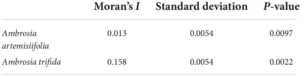
Table 2. Moran’s I test results of the spatial autocorrelation of the generalized linear model (GLM) residuals.

The spatial autocorrelation of the GLM residuals was tested using Moran’s I (Table 3) statistics. The P-values were statistically significant in both cases (P < 0.05). Hence, the residuals were spatially autocorrelated. Kriging was applied to reduce the uncertainty created by modeling variations that could not be modeled by the GLM with spatial autocorrelation of the residual.

TABLE 3

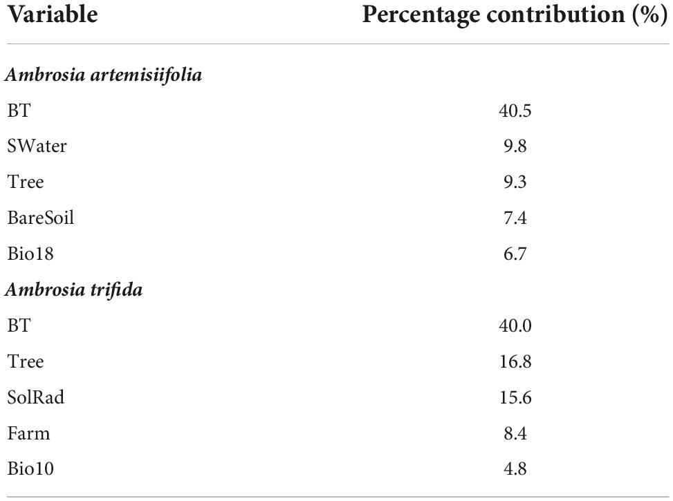
Table 3. Estimated contribution percent of the top five variables in the Maxent model.

Regression kriging

The GLM residuals were interpolated using kriging. The experimental variogram was fitted with the exponential variogram model (Figure 2). The variograms of the two species showed different patterns. For A. artemisiifolia, the effective range of the variogram was ca. 160 km (53.3 km × 3). The partial sill was 0.09, which was higher than that of the nugget (0.08). The spatial dependency remained in the study site. In contrast, the effective range of A. trifida’s variogram was 18 km (6.1 km × 3). However, the nugget of A. trifida (0.15) was higher than that of the partial sill (0.06). Thus, the variogram explains the higher variation in A. artemisiifolia than A. trifida. The nugget value is a pure error that is not modeled after kriging. A relatively high nugget value compared with the partial sill (modeled variation) indicates that there are significant pure errors.

FIGURE 2

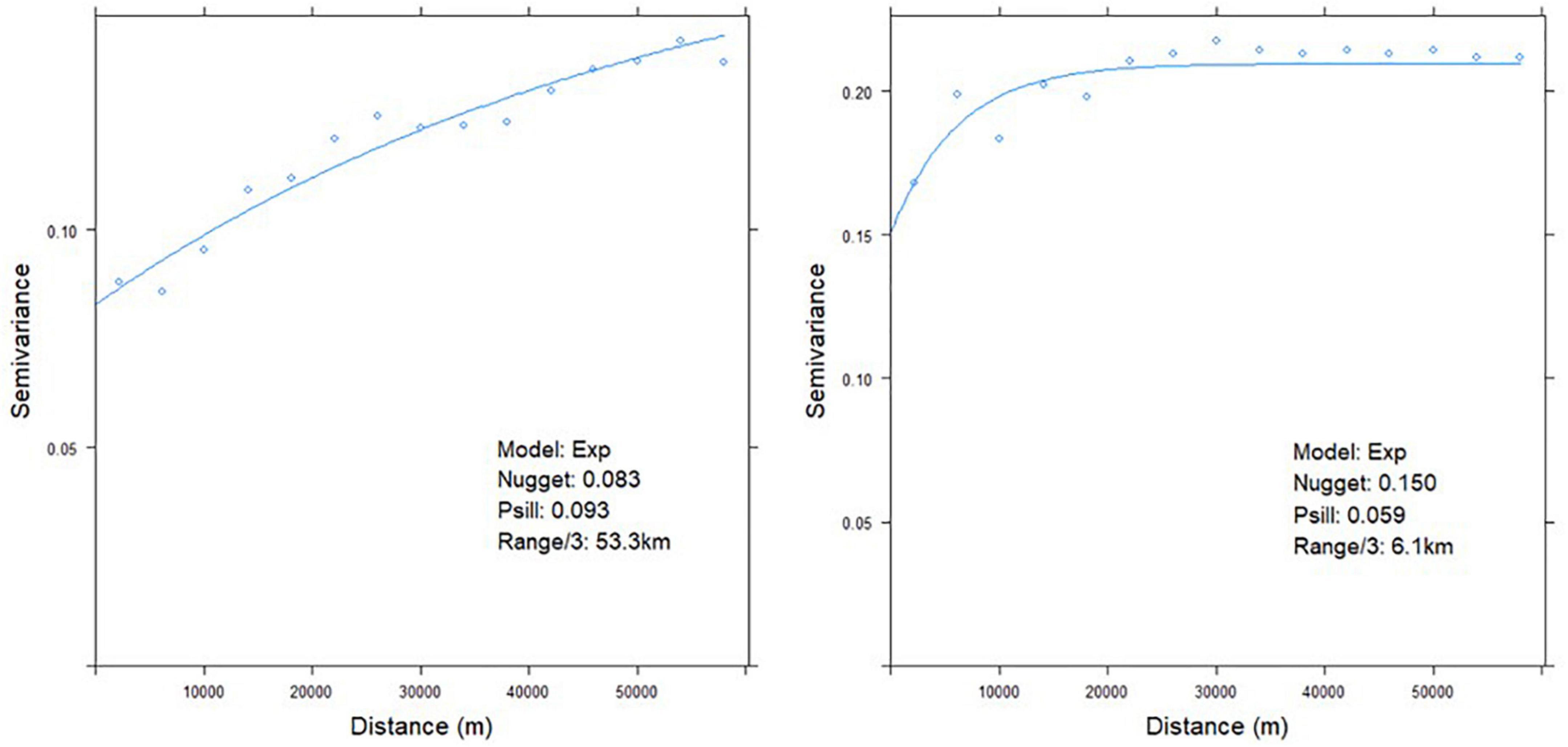
Figure 2. Fitted variogram mode of the generalized linear model (GLM) residuals (left: Ambrosia artemisiifolia, right: Ambrosia trifida).

The locations of the dataset were identical for both variograms. Nevertheless, the variograms differed because the species had different occurrence frequencies. Of the 1,035 training data points, 169 cells contained A. artemisiifolia, and 505 cells contained A. trifida. Moreover, the species differed in their distribution characteristics. A. trifida was widely distributed throughout the study site and A. artemisiifolia was mainly distributed in the south (Figure 1). These differences in spatial distribution may have caused the differences in the variogram ranges and sills.

The estimated values were back-transformed after RK. Thus, we predicted the probability of the species distribution within each cell (Figures 3, 4). For the RK models, the occurrence probability was estimated using environmental factors (GLM) and spatial autocorrelation (kriging). The probability of area surrounding the points where the species were observed was estimated to be higher than the probability evaluated by the GLM. The vicinity of the absence points had the opposite effect. To evaluate the performance of the model using RK, the ROC curve was plotted and the AUC value was calculated using the test data. The AUCs for A. artemisiifolia and A. trifida were 0.785 and 0.775, respectively (Figure 4). The AUC values were higher than the value recommended for a valid habitat model (0.75) (Elith, 2000). The Kappa coefficients for A. artemisiifolia and A. trifida were 0.473 and 0.461, respectively (Supplementary Table 2), while the TSS values were 0.525 and 0.465, respectively (Supplementary Table 2).

FIGURE 3

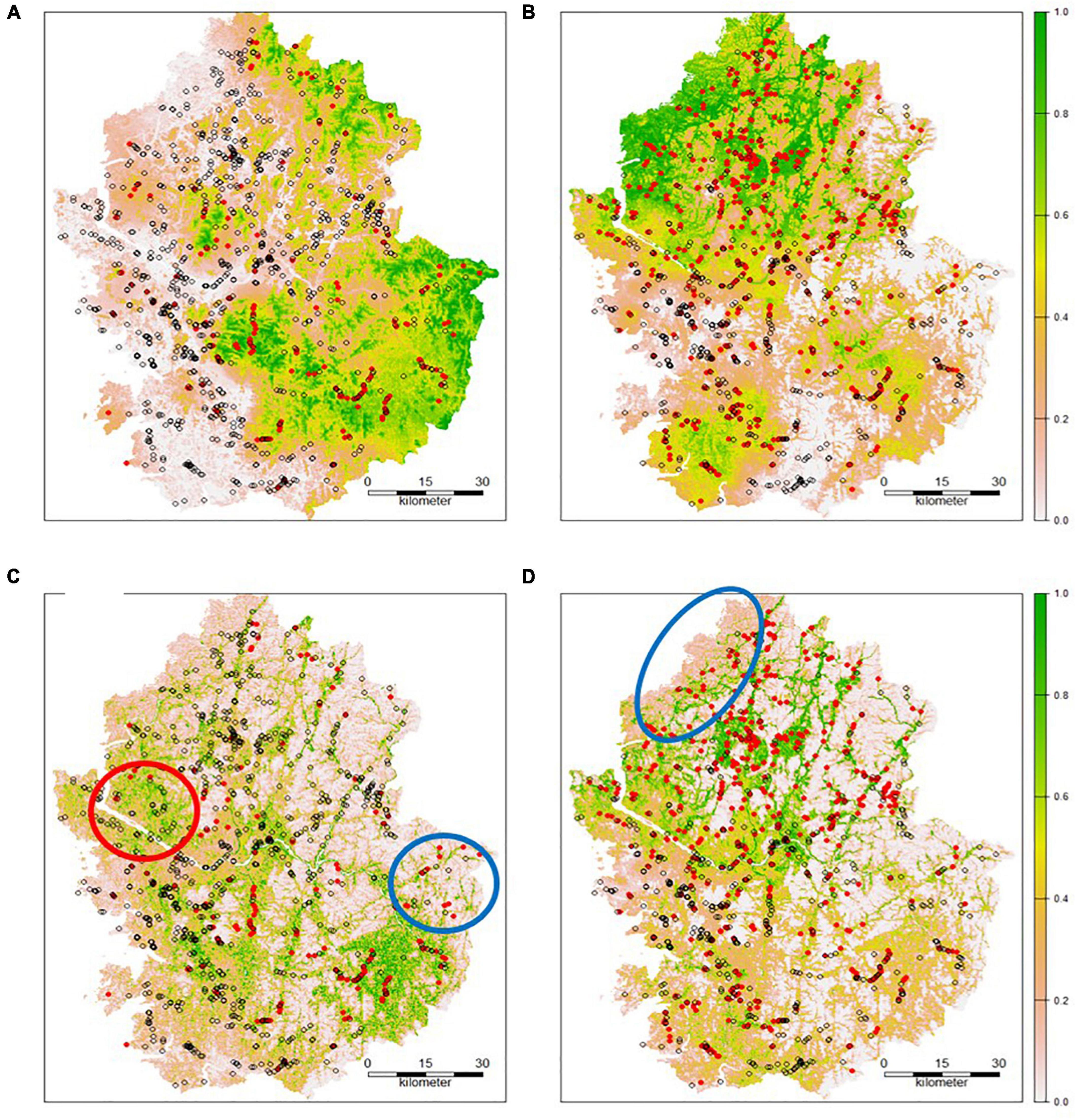
Figure 3. Predicted probability using an regression kriging (RK) model (A: Ambrosia artemisiifolia; B: Ambrosia trifida; red dot: presence; empty dot: absence; cross: test data point) and a Maxent model (C: A. artemisiifolia; D: A. Trifida).

FIGURE 4

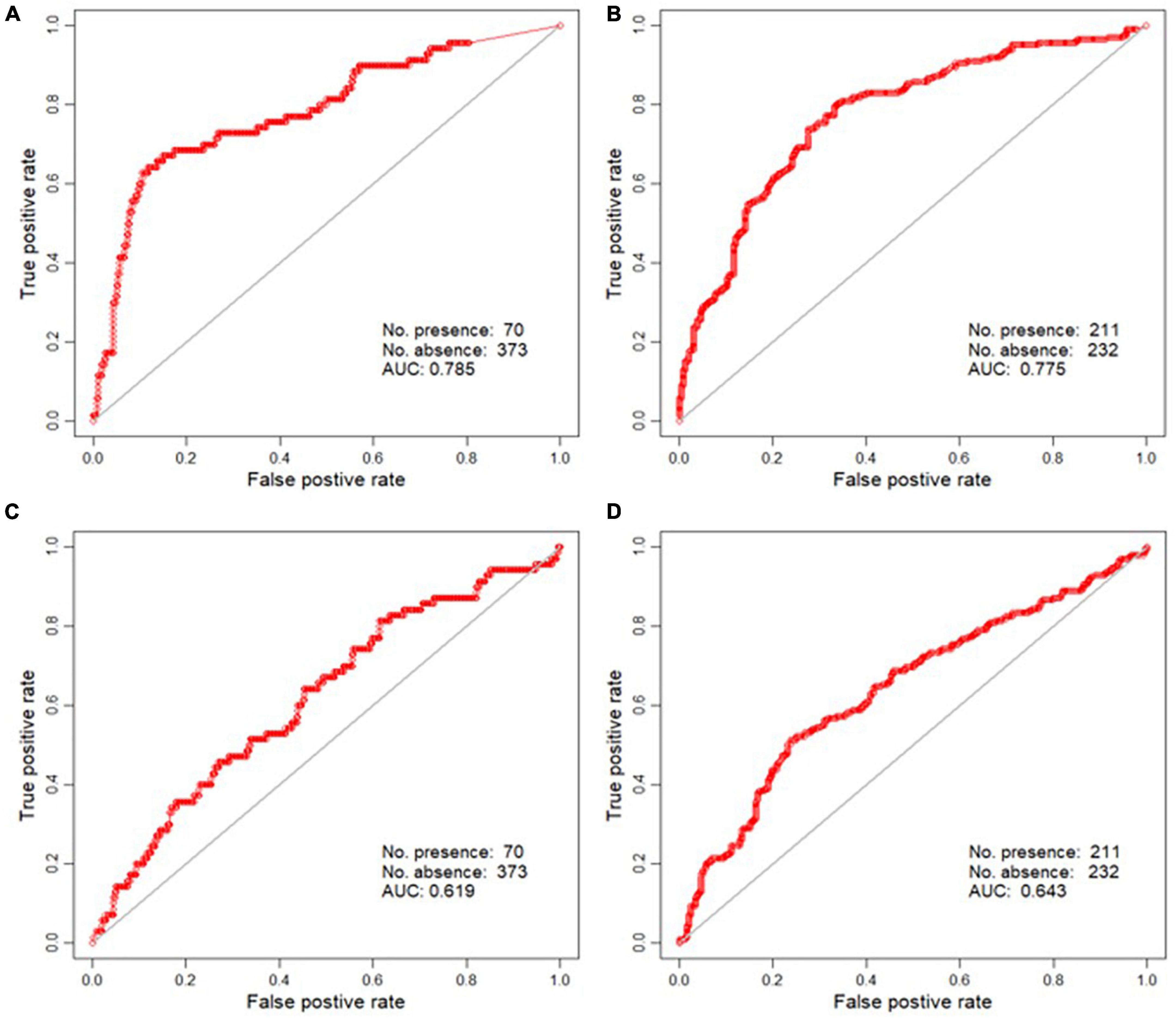
Figure 4. Receiver operating curve (ROC) plot of the regression kriging (RK) (A: Ambrosia artemisiifolia, B: Ambrosia trifida) and the Maxent result (C: A. artemisiifolia, D: A. trifida).

Maxent

Five environmental variables significantly contributed to the Maxent model (Table 3). The built-up area contributed the most to the models for both species. Tree cover contributed significantly to both models. However, the other variables contributed differently between the models (Table 3). The estimated habitat suitability index (HSI) is provided in Figure 3. The red circle in Figure 3C indicates a high HSI estimated by Maxent, but A. artemisiifolia was rarely observed in the area. The blue circles indicate low habitat suitability. Both species were observed in these unsuitable habitats (Figures 3C,D). The absence of species in areas with high habitat suitability may be due to many factors, such as dispersal restrictions and eradication efforts. However, numerous occurrences in areas with low habitat suitability were predicted, indicating a lack of predictive accuracy by the model.

When the Maxent model was evaluated using presence/background data, the AUC was 0.888 for A. artemisiifolia and 0.875 for A. trifida. However, when the Maxent model was evaluated using the independent P/A test data, the AUC for A. artemisiifolia was 0.619 and that for A. trifida was 0.643 (Figure 4). The low AUC summarizes the discrepancy between the predicted and observed distribution shown in Figure 3. The Kappa coefficients for A. artemisiifolia and A. trifida were 0.087 and 0.278, respectively (Supplementary Table 2), while the TSS values were 0.198 and 0.275, respectively (Supplementary Table 2).

Discussion

The Maxent and RK models were used to predict the spatial distributions of two invasive plant species A. artemisiifolia and A. trifida. Both species have had eradication targets since decades. We compared and analyzed the predictive performance of both models. The species differed in their prevalence and distribution but shared ruderal species traits. Thus, these species do not have strong habitat preferences. We modeled the spatial distribution of both species and evaluated the model performance using independent test data. The results indicated that RK outperformed Maxent. The AUC values of RK and Maxent were approximately 0.78 and 0.62, respectively.

Based on the standards proposed by Landis and Koch (1977), Kappa coefficient values ranging between 0.4 and 0.6 represent a moderate agreement strength, between 0.2 and 0.4 represent fair agreement strength, and between 0.01 and 0.2 represent marginal agreement strength. In our study, the RK model yielded better results than Maxent for the predictions of both species. Similar results were observed for TSS.

When investigating invasive species distributions, SDMs may not satisfy the niche hypothesis, which assumes that species may thrive relatively better in their preferred environmental conditions. A. artemisiifolia and A. trifida are typical cases. Maxent models the spatial distribution of diverse species, including invasive species (Lee et al., 2016; Park et al., 2017; Kim et al., 2018). In many studies, Maxent is a machine-learning model that outperforms other models (Elith et al., 2006). However, we observed a discrepancy between the predicted and observed data. It is well recognized that biased samples can degrade the performance of Maxent (Phillips et al., 2006; Elith et al., 2011), similar to the case of other SDMs. However, it is also true that unbiased data are difficult to obtain. Our data showed strong sampling bias (Figure 1). Surveys were usually conducted in easily accessible areas. In addition, Maxent may fail to model the relationship between environmental factors and habitat suitability when there is a weak habitat preference by the species (highly adaptable species) or unsaturated occupancy of the optimal environments. Using the same data in the RK model and Maxent, RK outperformed Maxent. Notably, an advantage of the GLM is that it uses P/A data. Although GLMs did not significantly reduce the deviances (Table 2), they alleviated the effect of sampling bias by modeling the P/A data. When both the presence and absence data are collected with the same degree of bias, the bias is offset (Elith et al., 2011). By contrast, Maxent uses presence-only and background data, and bias occurs only when the former data are used. Therefore, data bias strongly affects Maxent but not RK.

The present study shows that the built-up area fraction (BT) was negatively correlated with GLM and was the most important explanatory variable in Maxent (Table 3). The study area has the highest population density and urbanization level in Korea. This has increased the proportion of paved surfaces, which serves as a disadvantage for plant colonization of these regions. Both species are scarce in urban areas as they are known to be invasive and are continuously removed by locals.

In this study, the effective range of A. trifida was dominant compared to that of A. artemisiifolia. A. trifida occurs intensively in northwest South Korea, specifically in riversides and farmlands across the country, as the seeds disperse through flowing water (Lee et al., 2021). It is difficult for the two species to disperse long distances by wind because of their weight and morphological characteristics (Essl et al., 2015). Thus, these species are likely to exhibit spatial autocorrelation. Dong et al. (2020) reported that A. trifida showed higher rate of density increase than A. artemisiifolia, with increasing precipitation.

The distribution of A. trifida is positively associated with the precipitation of the Warmest Quarter and is restricted in northwest South Korea. Contrastingly, A. artemisiifolia was widely distributed. This indicated that A. trifida prefers more humid climate, and its dispersion is more difficult than A. artemisiifolia. A. artemisiifolia was observed in almost entire Europe, while A. trifida showed a regional distribution pattern (Chauvel et al., 2006, 2021; Cunze et al., 2013).

We predicted that A. artemisiifolia can disperse long distances more easily through vehicular transmission or other human activities on the roadside, but A. trifida mainly disperses through flowing water. Furthermore, compared with the habitat preferences of A. trifida, A. artemisiifolia prefers habitats with relatively drier soils and higher temperatures.

A. artemisiifolia and A. trifida are ruderal species. While their habitats are not markedly restricted, seed dispersal significantly limits their dispersal. Even when habitat suitability is low, an abundant seed supply from nearby clusters can form large colonies. Thus, the spatial distribution of both species was greatly affected by habitat suitability and spatial autocorrelation. The RK model accounts for spatial autocorrelation and can provide relatively better predictive performance than Maxent. For example, as shown in Figure 3, the RK model predicted low occurrence probability of A. artemisiifolia (red circular area in Figure 3A) because few A. artemisiifolia individuals were spotted in this area (empty dots dominated the area). However, Maxent did not account for the spatial context of data and predicted a high HSI in the study area (Figure 3C). Moreover, Maxent predicted a low HSI (blue circles in Figure 3), contrasting to the RK model.

The RK model can also map the uncertainty in prediction by calculating the kriging variation. Figure 5 demonstrates the kriging variance map of A. trifida. High values indicate a high predictive uncertainty. The kriging variance was low in areas with high survey point density, regardless of the observation value. When the density of survey points was limited, the values predicted through kriging were less reliable. The magnitude of the kriging variation may be affected by the survey point density and the variogram. Figure 5 shows that the uncertainty in the peripheral area was greater than in the inner area. Additional survey points could reduce the uncertainty of the kriging variance map of SDMs.

FIGURE 5

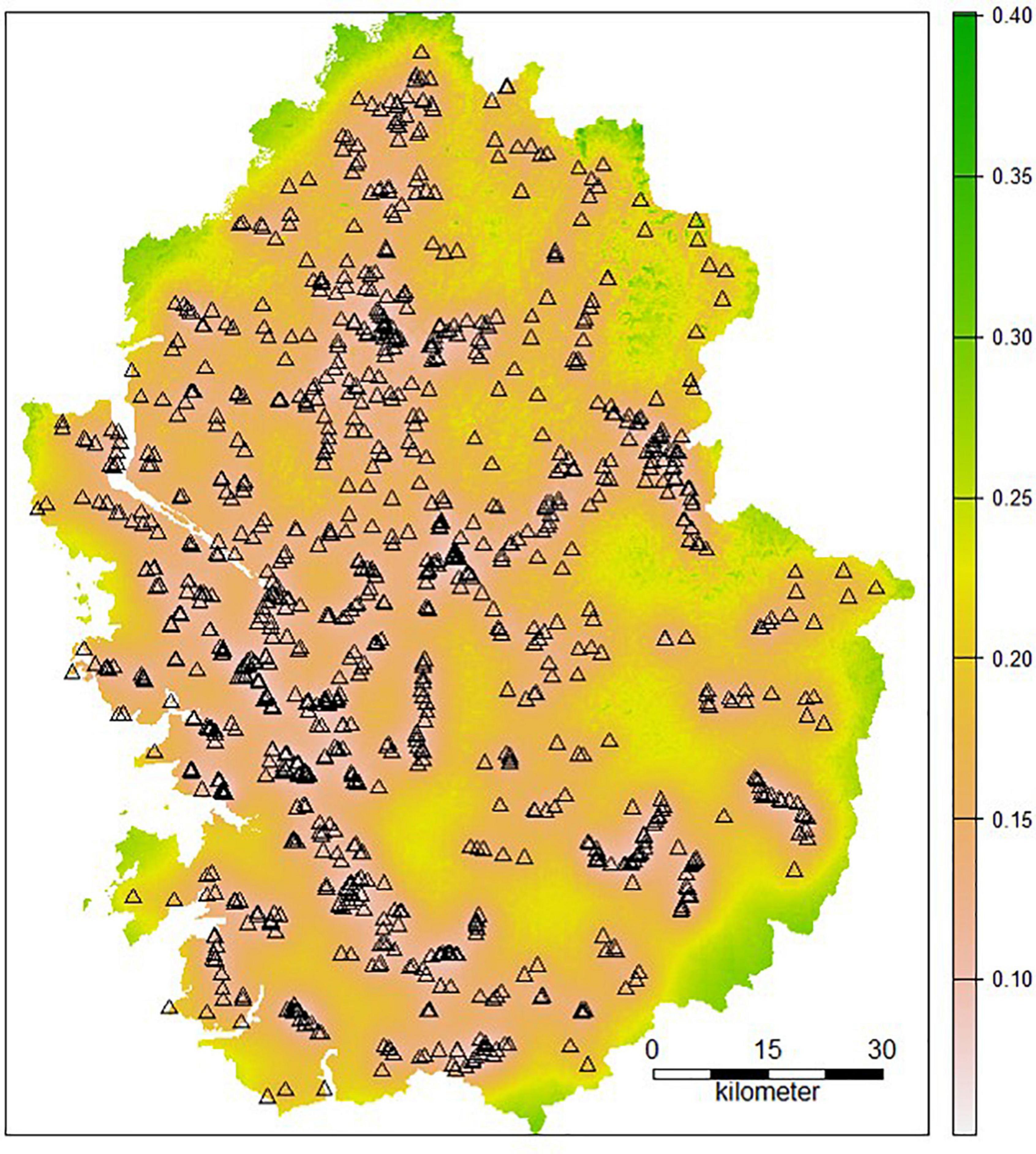
Figure 5. Regression kriging (RK) variance map of Ambrosia trifida (Triangles present sampling points).

Regression kriging can increase the prediction accuracy by modeling the real-world autocorrelation. For this reason, RK is widely used in various fields but not actively used in ecology. In the present study, the spatial distribution of invasive species was modeled using RK, which outperformed the model that did not consider spatial autocorrelation. A method for modeling the spatial distribution of invasive species using RK has been presented. This approach is not limited to studies targeting invasive species and can also be applied to model the spatial distribution of species that are difficult to predict based on the niche hypothesis.

Conclusion

Species distribution models model the relationships between environmental factors and species occurrence data based on the niche hypothesis and estimate the availability and preferences according to environmental conditions. For invasive species that rapidly disperse and disrupt ecosystems, the niche hypothesis is easily discarded by eradication activities or unsaturated dispersal. This weakens the predictive power of SDMs that are based on the niche hypothesis. In this study, we applied RK and Maxent to estimate the distribution of two invasive plant species, A. artemisiifolia and A. trifida. Both species are generalists and less affected by environmental restrictions; additionally, both are subjected to continuous eradication programs. To use RK, we initially modeled the relationship between the environmental factors and occurrence data using a GLM. We then modeled the residuals of the GLM by kriging. Modeling the spatial autocorrelation of the residuals using RK reduced the uncertainty of the model and enabled it to predict the spatial distribution of the species more accurately than Maxent. Habitat conditions and spatial dispersal constraints play important roles in determining the spatial distribution of a species. Therefore, RK, which can model both factors together, successfully predicted the spatial distribution of these invasive species.

Data availability statement

The original contributions presented in this study are included in the article/Supplementary material, further inquiries can be directed to the corresponding author.

Author contributions

KHC and D-HL designed the study. KHC and YSK performed the data collection, analysis, and manuscript writing. J-SP and JK supported with the experimental design. D-HL participated in the survey, reviewed the manuscript, and coordinated the overall research program. All authors have read and approved the final manuscript.

Funding

This research was supported by a grant from the Korea Environmental Industry & Technology Institute (2022003570001), funded by the Ministry of Environment and by the Basic Science Research Program through the National Research Foundation of Korea (NRF) (2020R1I1A1A01067345), and funded by the Ministry of Education in the Republic of Korea.

Conflict of interest

The authors declare that the research was conducted in the absence of any commercial or financial relationships that could be construed as a potential conflict of interest.

Publisher’s note

All claims expressed in this article are solely those of the authors and do not necessarily represent those of their affiliated organizations, or those of the publisher, the editors and the reviewers. Any product that may be evaluated in this article, or claim that may be made by its manufacturer, is not guaranteed or endorsed by the publisher.

Supplementary material

The Supplementary Material for this article can be found online at: https://www.frontiersin.org/articles/10.3389/fevo.2022.1036816/full#supplementary-material

Footnotes

1. ^ https://www.eorc.jaxa.jp/ALOS/en/index_e.htm
2. ^ https://www.worldclim.org

References

Allouche, O., Tsoar, A., and Kadmon, R. (2006). Assessing the accuracy of species distribution models: Prevalence, kappa and the true skill statistic (TSS). J. Appl. Ecol. 43, 1223–1232. doi: 10.1111/j.1365-2664.2006.01214.x

CrossRef Full Text | Google Scholar

Breiman, L., Friedman, J. H., Olshen, R. A., and Stone, C. J. (1984). “Classification and regression trees,” in Wadsworth statistics/probability, ed. Rouledge (London: Chapman & Hall/CRC).

Google Scholar

Buchhorn, M., Smets, B., Bertels, L., De Roo, B., Lesiv, M., Tsendbazar, N.-E., et al. (2020). Copernicus global land service: Land cover 100 m: Collection 3: Epoch 2019. Globe. Geneva: Zenodo.

Google Scholar

Chauvel, B., Dessaint, F., Cardinal-Legrand, C., and Bretagnolle, F. (2006). The historical spread of Ambrosia artemisiifolia L. in France from herbarium records. J. Biogeogr. 33, 665–673. doi: 10.1111/j.1365-2699.2005.01401.x

CrossRef Full Text | Google Scholar

Chauvel, B., Fried, G., Follak, S., Chapman, D., Kulakova, Y., Le Bourgeois, T., et al. (2021). Monographs on invasive plants in Europe N^° 5: Ambrosia trifida L. Bot. Lett. 168, 167–190. doi: 10.1080/23818107.2021.1879674

CrossRef Full Text | Google Scholar

Chun, Y. J., Nason, J. D., and Moloney, K. A. (2009). Comparison of quantitative and molecular genetic variation of native vs. invasive populations of purple loosestrife (Lythrum salicaria L., Lythraceae). Mol. Ecol. 18, 3020–3035. doi: 10.1111/j.1365-294X.2009.04254.x

PubMed Abstract | CrossRef Full Text | Google Scholar

Cohen, J. (1960). A coefficient of agreement for nominal scales. Educ. Psychol. Meas. 20, 37–46. doi: 10.1177/001316446002000104

CrossRef Full Text | Google Scholar

Cunze, S., Leiblein, M. C., and Tackenberg, O. (2013). Range expansion of Ambrosia artemisiifolia in Europe is promoted by climate change. ISRN Ecol. 2013:610126. doi: 10.1155/2013/610126

CrossRef Full Text | Google Scholar

Dai, J., Roberts, D. A., Stow, D. A., An, L., Hall, S. J., Yabiku, S. T., et al. (2020). Mapping understory invasive plant species with field and remotely sensed data in Chitwan, Nepal. Remote Sens. Environ. 250:112037. doi: 10.1016/j.rse.2020.112037

CrossRef Full Text | Google Scholar

Dong, H., Song, Z., Liu, T., Liu, Z., Liu, Y., Chen, B., et al. (2020). Causes of differences in the distribution of the invasive plants Ambrosia artemisiifolia and Ambrosia trifida in the Yili Valley, China. Ecol. Environ. 10, 13122–13133. doi: 10.1002/ece3.6902

PubMed Abstract | CrossRef Full Text | Google Scholar

Elith, J. (2000). “Quantitative methods for modeling species habitat: Comparative performance and an application to Australian plants,” in Quantitative methods for conservation biology, eds S. Ferson and M. Burgman (New York, NY: Springer), 39–58. doi: 10.1007/0-387-22648-6_4

CrossRef Full Text | Google Scholar

Elith, J. H., Graham, C. P., Anderson, R., Dudík, M., Ferrier, S., Guisan, A., et al. (2006). Novel methods improve prediction of species’ distributions from occurrence data. Ecography 29, 129–151. doi: 10.1111/j.2006.0906-7590.04596.x

CrossRef Full Text | Google Scholar

Elith, J., Phillips, S. J., Hastie, T., Dudík, M., Chee, Y. E., and Yates, C. J. (2011). A statistical explanation of MaxEnt for ecologists. Divers. Distrib. 17, 43–57. doi: 10.1111/j.1472-4642.2010.00725.x

CrossRef Full Text | Google Scholar

Elkind, K., Sankey, T. T., Munson, S. M., and Aslan, C. E. (2019). Invasive buffelgrass detection using highresolution satellite and UAV imagery on Google Earth Engine. Remote Sens. Ecol. Conserv. 5, 318–331. doi: 10.1002/rse2.116

CrossRef Full Text | Google Scholar

Essl, F., Biró, K., Brandes, D., Broennimann, O., Bullock, J. M., Chapman, D. S., et al. (2015). Biological flora of the British Isles: Ambrosia artemisiifolia. J. Ecol. 103, 1069–1098. doi: 10.1111/1365-2745.12424

CrossRef Full Text | Google Scholar

Essl, F., Lenzner, B., Bacher, S., Bailey, S., Capinha, C., Daehler, C., et al. (2020). Drivers of future alien species impacts: An expert-based assessment. Glob. Chang. Biol. 26, 4880–4893. doi: 10.1111/gcb.15199

PubMed Abstract | CrossRef Full Text | Google Scholar

Farashi, A., and Najafabadi, M. S. (2015). Modeling the spread of invasive nutrias (Myocastor coypus) over Iran. Ecol. Complex. 22, 59–64. doi: 10.1016/j.ecocom.2015.02.003

CrossRef Full Text | Google Scholar

Früh, L., Kampen, H., Kerkow, A., Schaub, G. A., Walther, D., and Wieland, R. (2018). Modeling the potential distribution of an invasive mosquito species: Comparative evaluation of four machine learning methods and their combinations. Ecol. Model. 388, 136–144. doi: 10.1016/j.ecolmodel.2018.08.011

CrossRef Full Text | Google Scholar

Fuller, D. A., Sasser, C. E., Johnson, W. B., and Gosselink, J. G. (1984). The effects of herbivory on vegetation on islands in Atchafalaya Bay, Louisiana. Wetlands 4, 105–114. doi: 10.1007/BF03160490

CrossRef Full Text | Google Scholar

Gioria, M., and Pyšek, P. (2016). The legacy of plant invasions: Changes in the soil seed bank of invaded plant communities. Bioscience 66, 40–53. doi: 10.1093/biosci/biv165

CrossRef Full Text | Google Scholar

Gioria, M., Pyšek, P., and Moravcova, L. (2012). Soil seed banks in plant invasions: Promoting species invasiveness and long-term impact on plant community dynamics. Preslia 84, 327–350.

Google Scholar

Google Maps (2021). Seoul capital area, Google Maps [Online]. Available online at: https://www.google.com/maps (accessed December 19, 2021).

Google Scholar

Gormley, A. M., Forsyth, D. M., Griffioen, P., Lindeman, M., Ramsey, D. S., Scroggie, M. P., et al. (2011). Using presence-only and presence-absence data to estimate the current and potential distributions of established invasive species. J. Appl. Ecol. 48, 25–34. doi: 10.1111/j.1365-2664.2010.01911.x

PubMed Abstract | CrossRef Full Text | Google Scholar

Hengl, T. (2020). GSIF: Global soil information facilities. R package version 0.5-5.1. Available online at: https://CRAN.R-project.org/package=GSIF

Google Scholar

Hengl, T., Heuvelink, G. B. M., and Rossiter, D. G. (2007). About regression-kriging: From equations to case studies. Comput. Geosci. 33, 1301–1315. doi: 10.1016/j.cageo.2007.05.001

CrossRef Full Text | Google Scholar

Hengl, T., Heuvelink, G. B. M., and Stein, A. (2004). A generic framework for spatial prediction of soil variables based on regression-kriging. Geoderma 120, 75–93. doi: 10.1016/j.geoderma.2003.08.018

CrossRef Full Text | Google Scholar

Hengl, T., Sierdsema, H., Radoviæ, A., and Dilo, A. (2009). Spatial prediction of species’ distributions from occurrence-only records: Combining point pattern analysis, ENFA and regression-kriging. Ecol. Model. 220, 3499–3511. doi: 10.1016/j.ecolmodel.2009.06.038

CrossRef Full Text | Google Scholar

Hinz, H. L., and Schwarzlaender, M. (2004). Comparing invasive plants from their native and exotic range: What can we learn for biological control? Weed Technol. 18, 1533–1541. doi: 10.1614/0890-037X(2004)018[1533:CIPFTN]2.0.CO;2

CrossRef Full Text | Google Scholar

Hong, S., Do, Y., Kim, J. Y., Kim, D.-K., and Joo, G.-J. (2015). Distribution, spread and habitat preferences of nutria (Myocastor coypus) invading the lower Nakdong River, South Korea. Biol. Invasions 17, 1485–1496. doi: 10.1007/s10530-014-0809-8

CrossRef Full Text | Google Scholar

Kil, J., Shim, K., Park, S., Koh, K., Suh, M., Ku, Y., et al. (2004). Distributions of naturalized alien plants in South Korea. Weed Technol. 18, 1493–1495. doi: 10.1614/0890-037X(2004)018[1493:DONAPI]2.0.CO;2

CrossRef Full Text | Google Scholar

Kim, A., Kim, Y.-C., and Lee, D.-H. (2018). A management plan according to the estimation of nutria (Myocastor coypus) distribution density and potential suitable habitat. J. Environ. Impact Assess. 27, 203–214.

Google Scholar

Kim, K. D. (2017). Distribution and management of the invasive exotic species Ambrosia trifida and Sicyos angulatus in the Seoul metropolitan area. J. Ecol. Eng. 18, 27–36. doi: 10.12911/22998993/76216

CrossRef Full Text | Google Scholar

Kim, Y.-H., Kil, J.-H., Hwang, S.-M., and Lee, C.-W. (2013). Spreading and distribution of Lactuca Scariola, invasive alien plant, by habitat types in Korea. Weed Turf. Sci. 2, 138–151. doi: 10.5660/WTS.2013.2.2.138

CrossRef Full Text | Google Scholar

Landis, J. R., and Koch, G. G. (1977). The measurement of observer agreement for categorical data. Biometrics 33, 184–186. doi: 10.2307/2529310

CrossRef Full Text | Google Scholar

Lee, D.-H., Lee, C.-W., and Kil, J. (2013). A study on plant diet resource of nutria (Myocastor coypus) habitat in Nakdong-river. J. Environ. Impact Assess. 22, 491–511. doi: 10.14249/eia.2013.22.5.491

CrossRef Full Text | Google Scholar

Lee, I., Kim, S., and Hong, S. J. (2021). Occurrence characteristics and management of Invasive weeds, Ambrosia artemisiifolia, Ambrosia trifida and Humulus japonicus. Weed Turf. Sci. 10, 227–242.

Google Scholar

Lee, S., Cho, K.-H., and Lee, W. (2016). Prediction of potential distributions of two invasive alien plants, Paspalum distichum and Ambrosia artemisiifolia, using species distribution model in Korean Peninsula. Ecol. Resil. Infrastruct. 3, 189–200. doi: 10.17820/eri.2016.3.3.189

CrossRef Full Text | Google Scholar

Mayfield, A. E., Seybold, S. J., Haag, W. R., Johnson, M. T., Kerns, B. K., Kilgo, J. C., et al. (2021). “Impacts of invasive species in terrestrial and aquatic systems in the United States,” in Invasive species in forests and rangelands of the United States: A comprehensive science synthesis for the United States forest sector, eds T. M. Poland, T. Patel-Weynand, D. M. Finch, C. F. Miniat, and D. C. Hayes (Heidelberg: Springer International Publishing), 5–39.

Google Scholar

Mills, E. L., Leach, J. H., Carlton, J. T., and Secor, C. L. (1994). Exotic species and the integrity of the Great Lakes: Lessons from the past. Bioscience 44, 666–676. doi: 10.2307/1312510

CrossRef Full Text | Google Scholar

Ministry of the Environment (2019). National mid-long term management plan of alien species. New Delhi: Ministry of the Environment.

Google Scholar

Ministry of the Environment and National Institute of Ecology (2018). Information for the field management of invasive alien species in Korea. New Delhi: Ministry of the Environment, National Institute of Ecology.

Google Scholar

Moran, P. A. P. (1950). Notes on continuous stochastic phenomena. Biometrika 37, 17–23. doi: 10.1093/biomet/37.1-2.17

CrossRef Full Text | Google Scholar

National Institute of Ecology (2019). Nationwide survey of non-native species in Korea. New Delhi: National Institute of Ecology.

Google Scholar

Ng, W. T., Candido de Oliveira Silva, A., Rima, P., Atzberger, C., and Immitzer, M. (2018). Ensemble approach for potential habitat mapping of invasive Prosopis spp. in Turkana, Kenya. Ecol. Evol. 8, 11921–11931. doi: 10.1002/ece3.4649

PubMed Abstract | CrossRef Full Text | Google Scholar

Odeh, I. O. A., McBratney, A. B., and Chittleborough, D. J. (1995). Further results on prediction of soil properties from terrain attributes: Heterotopic cokriging and regression-kriging. Geoderma 67, 215–226. doi: 10.1016/0016-7061(95)00007-B

CrossRef Full Text | Google Scholar

Park, H.-C., Lee, G.-G., and Lee, J.-H. (2015). Regional vulnerability assessment of invasive alien plants in Seoul and Gyeonggi Province. J. Korea Soc. Environ. Restor. Technol. 18, 1–13. doi: 10.13087/kosert.2015.18.6.1

CrossRef Full Text | Google Scholar

Park, H.-C., Lim, J.-C., Lee, J.-H., and Lee, G.-G. (2017). Predicting the potential distributions of invasive species using the Landsat imagery and Maxent: Focused on “Ambrosia trifida L. var. trifida” in Korean demilitarized zone. J. Korea Soc. Environ. Restor. Technol. 20, 1–12. doi: 10.13087/kosert.2017.20.1.1

CrossRef Full Text | Google Scholar

Phillips, S. J., Anderson, R. P., and Schapire, R. E. (2006). Maximum entropy modeling of species geographic distributions. Ecol. Model. 190, 231–259. doi: 10.1016/j.ecolmodel.2005.03.026

CrossRef Full Text | Google Scholar

Pimentel, D., Zuniga, R., and Morrison, D. (2005). Update on the environmental and economic costs associated with alien-invasive species in the United States. Ecol. Econ. 52, 273–288. doi: 10.1016/j.ecolecon.2004.10.002

CrossRef Full Text | Google Scholar

Prentis, P. J., Wilson, J. R., Dormontt, E. E., Richardson, D. M., and Lowe, A. J. (2008). Adaptive evolution in invasive species. Trends Plant Sci. 13, 288–294. doi: 10.1016/j.tplants.2008.03.004

PubMed Abstract | CrossRef Full Text | Google Scholar

QGIS Development Team (2020). QGIS geographic information system. Open source geospatial foundation project. QGIS Association.

Google Scholar

R Core Team (2020). R: A language and environment for statistical computing. R Foundation for statistical computing. Vienna: R Core Team.

Google Scholar

Rejmánek, M., and Randall, J. M. (1994). Invasive alien plants in California: 1993 summary and comparison with other areas in North America. Madrono 41, 161–177.

Google Scholar

Smolik, M. G., Dullinger, S., Essl, F., Kleinbauer, I., Leitner, M., Peterseil, J., et al. (2010). Integrating species distribution models and interacting particle systems to predict the spread of an invasive alien plant. J. Biogeogr. 37, 411–422. doi: 10.1111/j.1365-2699.2009.02227.x

CrossRef Full Text | Google Scholar

Tadono, T., Nagai, H., Ishida, H., Oda, F., Naito, S., Minakawa, K., et al. (2016). Generation of the 30-M-mesh global digital surface model by Alos prism. ISPRS Int. Arch. Photogramm. Remote Sens. Spat. Inf. Sci. XLI–B4, 157–162. doi: 10.5194/isprs-archives-XLI-B4-157-2016

CrossRef Full Text | Google Scholar

Vilà, M., Espinar, J. L., Hejda, M., Hulme, P. E., Jarošík, V., Maron, J. L., et al. (2011). Ecological impacts of invasive alien plants: A meta-analysis of their effects on species, communities and ecosystems. Ecol. Lett. 14, 702–708. doi: 10.1111/j.1461-0248.2011.01628.x

PubMed Abstract | CrossRef Full Text | Google Scholar

Ward, D. F. (2007). Modeling the potential geographic distribution of invasive ant species in New Zealand. Biol. Invasions 9, 723–735. doi: 10.1007/s10530-006-9072-y

CrossRef Full Text | Google Scholar

Warziniack, T., Haight, R. G., Yemshanov, D., Apriesnig, J. L., Holmes, T. P., Countryman, A. M., et al. (2021). “Economics of invasive species,” in Invasive species in forests and rangelands of the United States: A comprehensive science synthesis for the United States Forest sector, eds T. Patel-Weynand, D. M. Finch, C. F. Miniat, and D. C. Hayes (Heidelberg: Springer International Publishing), 305–320. doi: 10.1007/978-3-030-45367-1_14

CrossRef Full Text | Google Scholar