Artificial intelligence carbon neutrality strategy in sports event management based on STIRPAT-GRU and transfer learning

1 Introduction

The development of renewable energy technologies has become a major global concern due to the negative impact of greenhouse gases on the environment and human health. In recent years, there has been growing interest in the application of machine learning and deep learning techniques to optimize renewable energy systems and reduce carbon emissions Elnour et al. (2022a). The optimization of renewable energy systems is crucial in promoting sustainability and reducing carbon emissions Wicker (2018). Machine learning and deep learning techniques offer a promising approach to achieve this by improving the accuracy of predictions and optimizing system performance. Commonly used machine learning and deep learning models as follows:

Support Vector Machines (SVM) Abdou et al. (2022): SVM is a popular machine learning algorithm used for classification and regression tasks. It works by finding the optimal hyperplane that separates the data into different classes. SVM is effective in handling large datasets and can handle both linear and non-linear data. One of the key advantages of SVM is its ability to handle high-dimensional data and find the most relevant features. However, SVM can be computationally expensive and may not be suitable for real-time applications.

Random Forest (RF) Zhuang et al. (2022): RF is a decision tree-based algorithm that combines multiple decision trees to improve prediction accuracy. Each decision tree in the forest is trained on a random subset of the data and features. RF is effective in handling missing data and is robust to noise. It can also handle both classification and regression tasks. However, RF can be susceptible to overfitting and may not be suitable for high-dimensional data.

Artificial Neural Networks (ANN) Kong et al. (2021): ANN is a deep learning model that simulates the structure and function of the human brain. It consists of multiple layers of interconnected nodes that process and transform input data. ANN is effective in handling complex tasks and is capable of learning from large datasets. It can handle both classification and regression tasks and can be used for image, speech, and text recognition tasks. However, ANN can be computationally expensive and requires a large amount of training data.

Convolutional Neural Networks (CNN) Xu et al. (2023): CNN is a deep learning model commonly used in image recognition tasks. It works by applying convolutional filters to the input data to extract features. The extracted features are then passed through multiple layers of interconnected nodes for further processing. CNN is effective in handling high-dimensional data and is capable of learning complex features. It is commonly used for object detection, image classification, and image segmentation tasks. However, CNN may not be suitable for non-image data.

Recurrent Neural Networks (RNN) Liu et al. (2022): RNN is a deep learning model commonly used in sequential data analysis tasks. It works by processing input data in a time-dependent manner, allowing it to model temporal dependencies. RNN is effective in handling variable-length input sequences and can handle both classification and regression tasks. It is commonly used for speech recognition, natural language processing, and time-series analysis tasks. However, RNN can be susceptible to vanishing gradients, which can affect its ability to model long-term dependencies.

In recent years, models based on the Transformer architecture have garnered widespread attention and achieved remarkable success in natural language processing and other fields Vaswani et al. (2017). Take the BERT (Bidirectional Encoder Representations from Transformers) model as an example; it has excelled in natural language understanding tasks and revolutionized text processing methods. Furthermore, several optimization algorithms have provided us with better ways to search for parameter combinations, such as the Whale Optimization Algorithm (WOA). These algorithms not only assist in optimizing the performance of deep learning models but also facilitate parameter tuning and hyperparameter search, thus enhancing model efficiency and accuracy. These developments have not only found potential applications in carbon neutrality strategies but have also opened up new opportunities and prospects for artificial intelligence in various domains. They equip us with more tools and methods to address complex environmental and sustainability challenges, contributing significantly to building a smarter and more sustainable future.

However, these traditional methods are prone to overfitting, and training on large-scale datasets requires a significant amount of time, memory, and computational resources. To solve this problem, this paper proposes a method based on the STIRPAT-GRU and Transfer Learning. This paper employ the Stochastic Impacts by Regression on Population, Affluence and Technology (STIRPAT) model Chekouri et al. (2020) as the initial step in our methodology. The STIRPAT model is a widely recognized framework that allows us to understand the relationship between carbon emissions and population, wealth, and technology factors. By analyzing historical data and conducting statistical analysis, the STIRPAT model enables us to identify the key drivers of carbon emissions in sports events. Then employ the Gated Recurrent Unit (GRU) Himeur et al. (2022) neural network to develop a predictive model. The GRU is a type of recurrent neural network that excels in capturing temporal dependencies and patterns. By training the GRU model, we can accurately forecast future trends and patterns of carbon emissions in sports event management. Lastly, introduce transfer learning Zhang et al. (2023) into our methodology to enhance the accuracy and robustness of the predictive model. Transfer learning leverages knowledge and experience gained from other domains to improve the performance of the model in the specific context of sports event management. The proposed method provides a comprehensive and data-driven approach to analyze and predict carbon emissions in sports event management. The integration of these techniques allows us to not only identify the key drivers of carbon emissions but also forecast future trends, patterns, and potential mitigation strategies.

Below are contributions of this paper:

● The method proposed an AI-based carbon neutrality strategy using the STIRPAT model, GRU neural network, and transfer learning to predict carbon emissions trends and patterns in sports events, helping sports event managers develop data-driven carbon neutrality strategies.

● Revealed the impact of population, wealth, and technology on carbon emissions and predicted future trends and patterns of carbon emissions in sports events using the STIRPAT model and GRU neural network.

● Provided a data-driven approach for sports event managers to manage carbon emissions using artificial intelligence and deep learning techniques, promoting the development of a more sustainable and environmentally friendly sports industry.

In the remaining sections of this paper, we will introduce recent related work in Section 2. Section 3 presents our used method: STIRPAT, GRU, and Transfer Learning. The experimental part, details, and comparative experiments are discussed in Section 4. Finally, Section 5 concludes the paper.

2 Related work

2.1 Fuzzy C-means clustering and Support Vector Machine

Fuzzy C-means clustering and Support Vector Machine (FCS-SVM) model Xu and Song (2019) is a method that combines fuzzy C-means clustering and Support Vector Machine for carbon emission prediction. The main steps of this model are as follows:

● Data preprocessing: Firstly, collect data related to carbon emissions such as past carbon emission data, economic indicators, population data, etc. Then preprocess the data, including filling missing values, handling outliers, and normalizing the data to ensure data quality and consistency.

● Fuzzy C-means clustering: Use the fuzzy C-means clustering algorithm to cluster the preprocessed data. This step aims to divide the samples into multiple clusters that belong to different categories,

● where each cluster represents a collection of samples with similar characteristics.

● Feature extraction: Within each clustered cluster, relevant indicators representing the features of the cluster can be extracted. These features can be factors closely related to carbon emissions, such as industrial output, energy consumption, etc.

● Support Vector Machine (SVM) modeling: Use Support Vector Machine to model the data within each clustered cluster as training samples. SVM is a supervised learning algorithm used for classification and regression problems. Here, SVM is used to establish a carbon emission prediction model related to the features.

● Carbon emission prediction: When new data enters the model, the model will classify it into the corresponding cluster based on its features, and then use the corresponding SVM model to predict the carbon emissions under that category.

The advantages of the FCS-SVM model in carbon emission prediction include: improved prediction accuracy by combining fuzzy C-means clustering and support vector machine (SVM) to consider both sample similarity and non-linear relationships; the ability to make accurate predictions with limited data due to SVM’s performance in high-dimensional spaces even with a small amount of data; and flexibility in adapting to data changes by adding or removing clustering clusters. However, the FCS-SVM model has the following disadvantages: parameter adjustment and optimization are required for model establishment, which may require experience and time; the model’s training and prediction speed may be slow when dealing with large-scale data, especially during fuzzy C-means clustering; and it may struggle to adapt well to the complexity of very complex datasets, resulting in less accurate predictions.

2.2 Extreme Learning Machine

In the field of carbon emission prediction, the Extreme Learning Machine (ELM) model Zheng et al. (2022) has received widespread attention and research as a fast and efficient machine learning method. Many research papers and literature have explored the application of the ELM model in carbon emission prediction. These studies cover carbon emission predictions in different industries, cities, and countries, as well as predictions at different time scales, ranging from hourly to annual levels. Data sources for carbon emission prediction include carbon emission databases, energy consumption data, economic statistics data, etc. The ELM model is commonly used to handle these large-scale datasets and predict carbon emissions quickly and accurately. Some recent research work has improved and optimized the ELM model to enhance its predictive performance. For example, by combining the ELM model with other models such as ARIMA Solarin et al. (2019), LSTM Elnour et al. (2022b), or incorporating domain-specific prior knowledge to improve the model’s accuracy. Carbon emissions are influenced by various factors such as industrial production, energy consumption, transportation, etc. Researchers often combine the ELM model with models related to other factors to form a multi-factor prediction model to comprehensively consider the complexity of carbon emissions. Some studies aim to utilize the ELM model for real-time carbon emission prediction to support governments and businesses in formulating carbon reduction policies and decision-making. Carbon emission prediction is an interdisciplinary field that requires the integration of knowledge from environmental science, economics, statistics, and other disciplines. The application of the ELM model also promotes interdisciplinary collaboration to better understand and address the issue of carbon emissions.

The ELM model Zhao et al. (2023) has several advantages. It has a very fast training speed due to its use of analytical solutions for weight determination, avoiding iterative optimization. Moreover, it exhibits high generalization capability, performing well on both training and new data, preventing overfitting. It is also highly scalable, making it suitable for large datasets and complex problems. However, the ELM model also has some limitations. The number of hidden layer nodes and activation function choice may affect predictive performance, requiring tuning through methods like cross-validation. It may not be suitable for complex problems, as more complex models like deep neural networks could perform better in handling nonlinear and complex data. Additionally, the random initialization of hidden layer nodes’ weights and biases may lead to different results under different initialization conditions.

2.3 Backpropagation Neural Network

The Backpropagation Neural Network (BPNN) model Onyelowe et al. (2023) is a common artificial neural network model used for solving classification and regression problems. It consists of an input layer, hidden layers, and an output layer. Through forward propagation, input data is passed from the input layer to the output layer, and predictions are calculated. Then, by comparing the predictions with the true values, the weights and biases in the network are adjusted through backpropagation to minimize the loss function and improve the predictive accuracy of the model.

In the field of carbon mitigation, the BPNN model Ahmed et al. (2021) is widely recognized and extensively utilized for its effectiveness in various tasks. One prominent application is carbon emission prediction, where the BPNN model proves invaluable. By leveraging historical data, the model learns intricate patterns and trends, enabling it to make accurate predictions about future carbon emissions. This capability is essential for policymakers, environmental analysts, and organizations seeking to assess and manage their carbon footprint, allowing them to develop informed strategies and policies for carbon reduction. Another area where the BPNN model demonstrates its utility is in the analysis of carbon trading markets. With its ability to capture complex relationships and non-linear dynamics, the model can effectively analyze price fluctuations and trends within these markets. This analysis provides valuable insights into market behavior, facilitating decision-making processes for investors, traders, and regulators. By understanding the underlying factors influencing carbon market dynamics, stakeholders can optimize their trading strategies, assess market risks, and identify opportunities for carbon offsetting or investments in low-carbon technologies.

Advantages of the BPNN model Zhang et al. (2021) include its ability to learn and adapt to nonlinear relationships, making it suitable for complex carbon mitigation problems. It has strong generalization capability, handling multi-dimensional features and large-scale datasets. Once trained, the model can make predictions quickly. However, the BPNN model also has some disadvantages. Training time may be long for large-scale datasets and complex network structures. The performance of the model highly depends on the selection of initial weights and biases, which may require multiple training runs to obtain the best results. It is prone to getting stuck in local minima and may not reach the global optimal solution.

3 Methodology

3.1 Overview of our network

The proposed research aims to develop an AI-powered carbon neutrality strategy for sports event management using a combination of the STIRPAT-GRU model and transfer learning. The STIRPAT-GRU model is used to identify the key drivers of carbon emissions and predict future trends and patterns, while transfer learning is used to improve the accuracy and robustness of the model. Figure 1 is the overall flow chart.

FIGURE 1

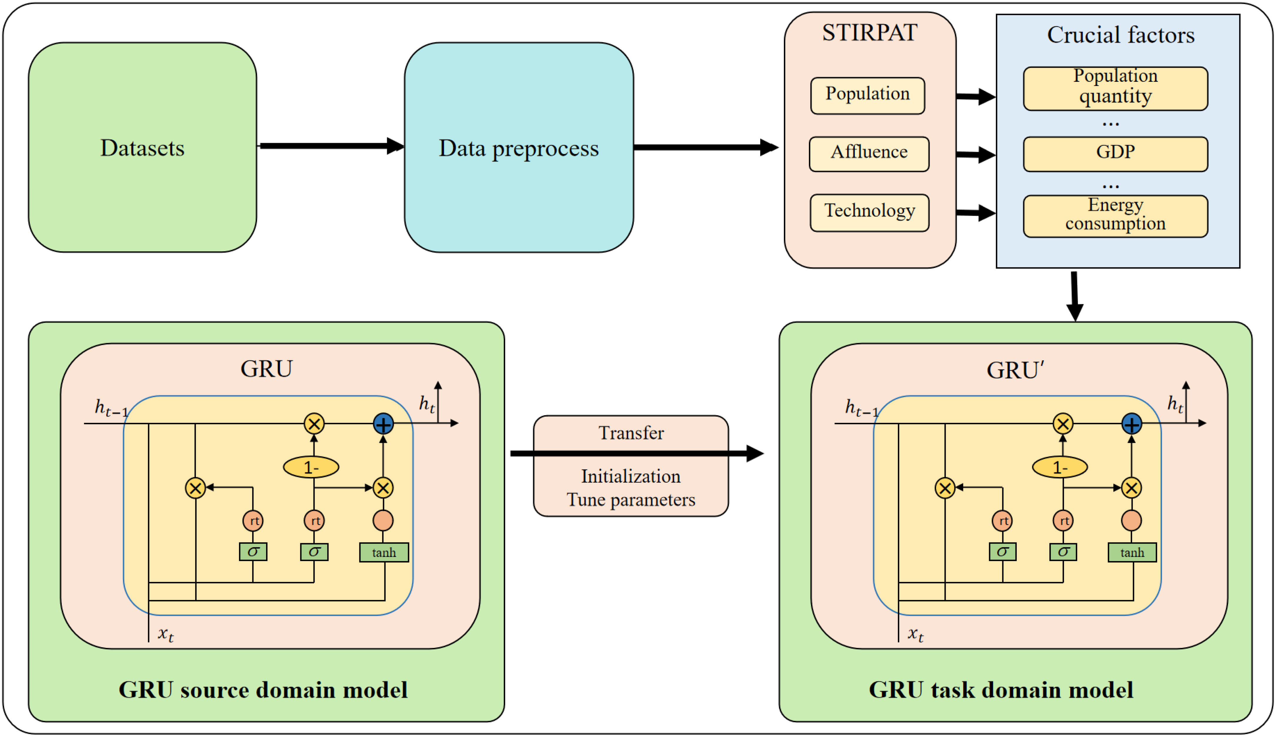
Figure 1 Overall flow chart of the model.

The STIRPAT-GRU model combines the STIRPAT model, which is a statistical model that analyzes the drivers of environmental impact, with the GRU neural network, which captures the temporal dependencies in sequential data. The model analyzes the impact of population, wealth, and technology on carbon emissions in sports events and predicts future trends and patterns. Transfer learning is a machine learning technique that involves training a model on one task and then fine-tuning it for another related task. In the context of sports event management, transfer learning is used to improve the accuracy and robustness of the STIRPAT-GRU model by leveraging knowledge and experience gained from other domains.

The proposed research includes several steps: data collection and preprocessing, Model training, evaluation. Firstly, collect datasets on carbon emissions in sports events, cleaning and formatting it to ensure its consistency and reliability for analysis. Secondly, develop the STIRPAT model to analyze the impact of population, wealth, and technology on carbon emissions in sports events. Develop the GRU neural network to forecast future trends and patterns of carbon emissions in sports events. Fine-tune the STIRPAT-GRU model using transfer learning to improve its accuracy and robustness. Thirdly, evaluate the effectiveness of the proposed approach and compare it with other methods.

The proposed approach is expected to provide sports event managers with valuable insights into carbon emissions and promote sustainability in the sports industry.

3.2 Stochastic impacts by regression on population, affluence and technology

The STIRPAT model Gani (2021) is an empirical model used to analyze environmental impacts, named after the variables used in the model, including population, affluence, technology, and politics, among others. The basic principle of the STIRPAT model is to establish a relationship model between the factors that influence human activity and environmental impacts, in order to predict the impact of human activity on the environment. The population factor in the model mainly includes factors such as population size and population growth rate, while the affluence factor mainly includes factors such as per capita GDP and consumption level. The technology factor mainly includes factors such as energy efficiency and technological progress, while the politics factor mainly includes factors such as policy measures and social values. By quantifying and analyzing these factors, a mathematical model describing the impact of human activities on the environment can be established. In practical applications, the STIRPAT model can be used to predict the impact of human activities on the environment, such as predicting carbon emissions, energy consumption, and water resource utilization. The main function of the STIRPAT model is to provide a method for analyzing the impact of human activities on the environment, which can provide decision support and guidance for environmental protection and sustainable development. At the same time, the model can also be used to evaluate the impact of different policies, technologies, and social development paths on the environment, thereby providing more scientific and reliable decision-making basis. As shown in Figure 2, it is the flow chart of STIRPAT model:

FIGURE 2

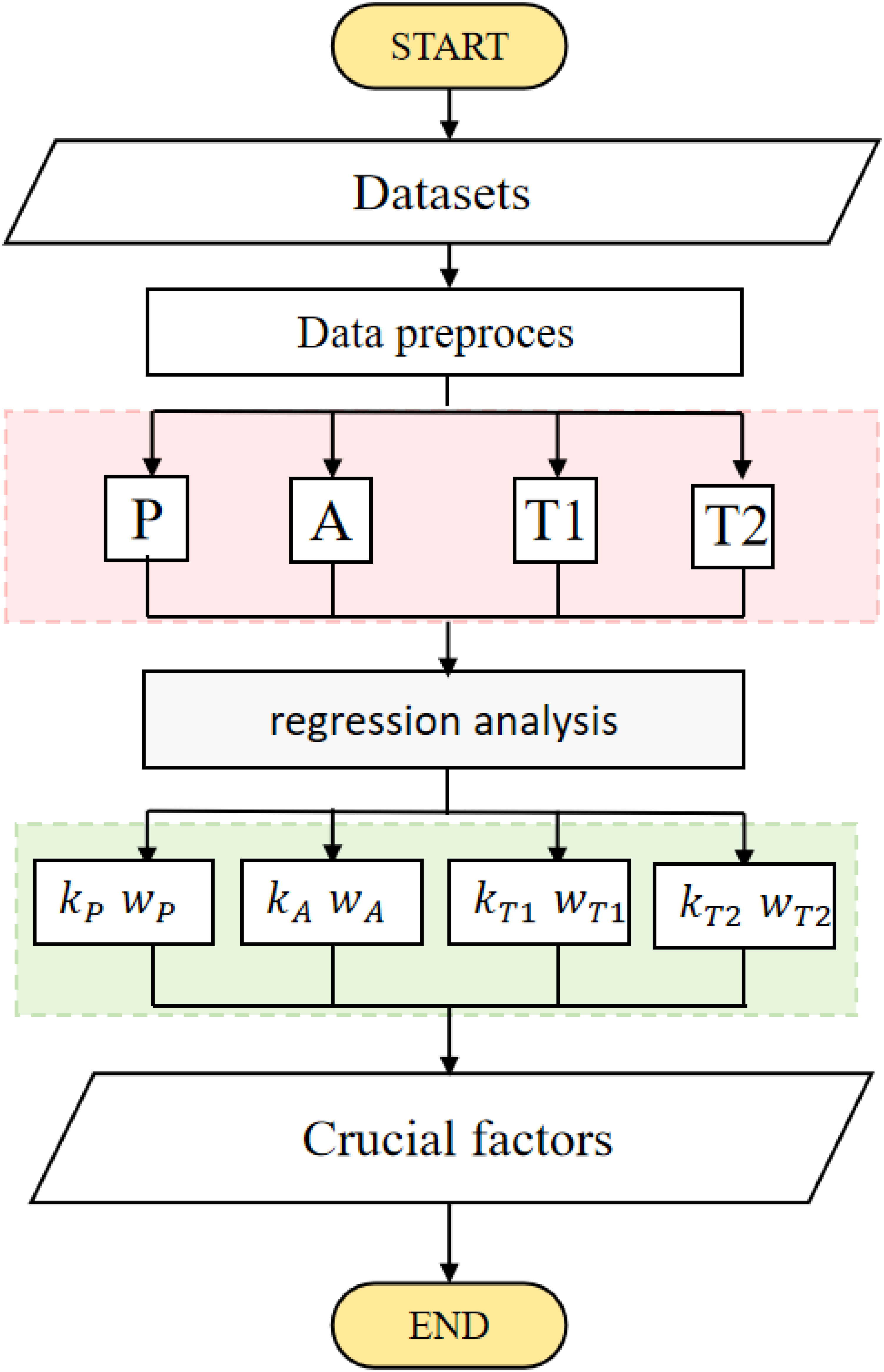
Figure 2 Flow chart of the STIRPAT model.

The equations for the STIRPAT model Yang et al. (2021) are as follows:

$\begin{array}{ll}I=P\times A\times T& (1)\end{array}$

Here, I represents environmental impact, P represents population factor, A represents affluence factor, and T represents technology factor.

The population factor can be expressed as:

$\begin{array}{ll}P=P_0\times {\left(\frac{G}{G_0}\right)}^{{\beta }_G}\times {\left(\frac{E}{E_0}\right)}^{{\beta }_E}& (2)\end{array}$

Here, P₀ represents the baseline population, G represents per capita GDP, G₀ represents the baseline per capita GDP, E represents energy consumption, E₀ represents the baseline energy consumption, and β_G and β_E are regression coefficients.

The affluence factor can be expressed as:

$\begin{array}{ll}A={\left(\frac{G}{G_0}\right)}^{\alpha G}\times {\left(\frac{E}{E_0}\right)}^{\alpha E}& (3)\end{array}$

Here, α_G and α_E are regression coefficients.

The technology factor can be expressed as:

$\begin{array}{ll}T={\left(\frac{G}{G_0}\right)}^{\gamma G}\times {\left(\frac{E}{E_0}\right)}^{\gamma E}& (4)\end{array}$

Here, γ_G and γ_E are regression coefficients.

The model assumes that environmental impact can be explained by the product of population, affluence, technology, and the environmental impact factor. The environmental impact factor can include factors such as energy consumption, waste emissions, land use, depending on the specific environmental issue being studied and data availability.

3.3 Gated recurrent unit

The GRU model Choe et al. (2021) is a type of RNN used for processing sequential data, such as natural language, speech, and time series data. Compared to traditional RNN models, the GRU model has better information retention and training efficiency. The GRU model is based on a gate mechanism that controls the flow and forgetting of information. This mechanism helps the GRU model to better remember relevant information in the input sequence and can reduce the problem of vanishing gradients, improving the model’s training efficiency. The GRU model consists of two gate units: an update gate and a reset gate. The update gate is used to control whether the hidden state at the current time step should be updated, helping the model to identify which information in the sequence is important. The reset gate is used to control whether the new input at the current time step and the hidden state from the previous time step should be mixed, helping the model to forget irrelevant information. The advantages of the GRU model include its ability to maintain good performance when processing long sequence data, while avoiding the vanishing gradient problem that exists in traditional RNN models. The GRU model is widely used in natural language processing, speech recognition, and time series prediction, among other fields. As shown in Figure 3, it is the flow chart of GRU model:

FIGURE 3

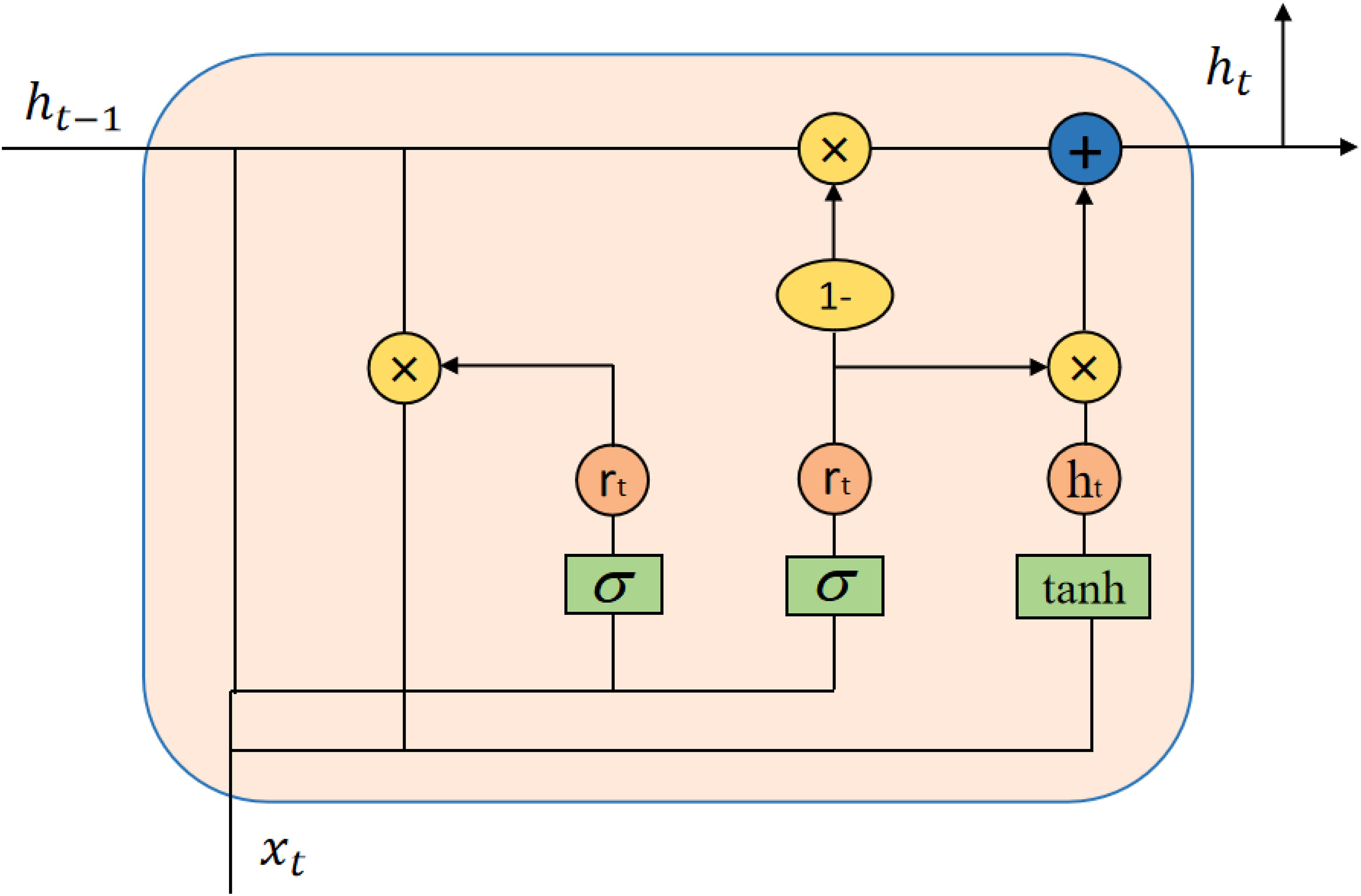
Figure 3 Flow chart of the GRU model.

The equations for the GRU model Rouhi Ardeshiri and Ma (2021) are as follows:

$\begin{array}{ll}{h}_t=(1-z_t)\odot h_{t-1}+z_t\odot {\tilde{h}}_t& (5)\end{array}$

Here, h_t represents the hidden state at the current time step, z_t is the value of the update gate, ${\tilde{h}}_t$ is the candidate hidden state at the current time step, and ⊙ denotes element-wise multiplication.

The update gate is calculated as follows:

$\begin{array}{ll}{z}_t=\sigma (W_z{x}_t+U_z{h}_{t-1})& (6)\end{array}$

Here, W_z and U_z are the weight matrices of the update gate, σ is the Sigmoid function, and x_t is the input at the current time step.

The candidate hidden state is calculated as follows:

$\begin{array}{ll}\tilde{h}t=\tanh (W{x}_t+r_t\odot Uht-1)& (7)\end{array}$

Here, W and U are the weight matrices of the candidate hidden state, and r_t is the value of the reset gate. The reset gate is calculated as follows:

$\begin{array}{ll}{r}_t=\sigma (W_r{x}_t+U_r{h}_{t-1})& (8)\end{array}$

Here, W_r and U_r are the weight matrices of the reset gate.

In sports event management, the GRU model can be used to predict the trend and pattern of carbon emissions. By analyzing historical data and current environmental factors, a GRU model can be trained to predict future carbon emission trends and patterns, providing guidance and suggestions for reducing carbon emissions and achieving carbon neutrality.

3.4 Transfer learning

Transfer learning Sayed et al. (2022) is a machine learning method that aims to transfer knowledge learned in one task to a new task in order to improve the performance of the model on the new task. The goal of transfer learning is to leverage the knowledge learned in the source domain to help solve problems in the target domain. The main idea of transfer learning is to improve the generalization ability of the model on the target domain by utilizing the commonalities and differences between the source domain and the target domain. Transfer learning can be divided into three types: instance-based transfer learning, feature-based transfer learning, and model-based transfer learning. Instance-based transfer learning directly applies instances from the source domain to the target domain to improve the performance of the model on the target domain. Feature-based transfer learning extracts common features between the source and target domains to learn a new model on the target domain. Model-based transfer learning learns a general model in the source domain and fine-tunes it in the target domain. As shown in Figure 4, it is the flow chart of Transfer Learning:

FIGURE 4

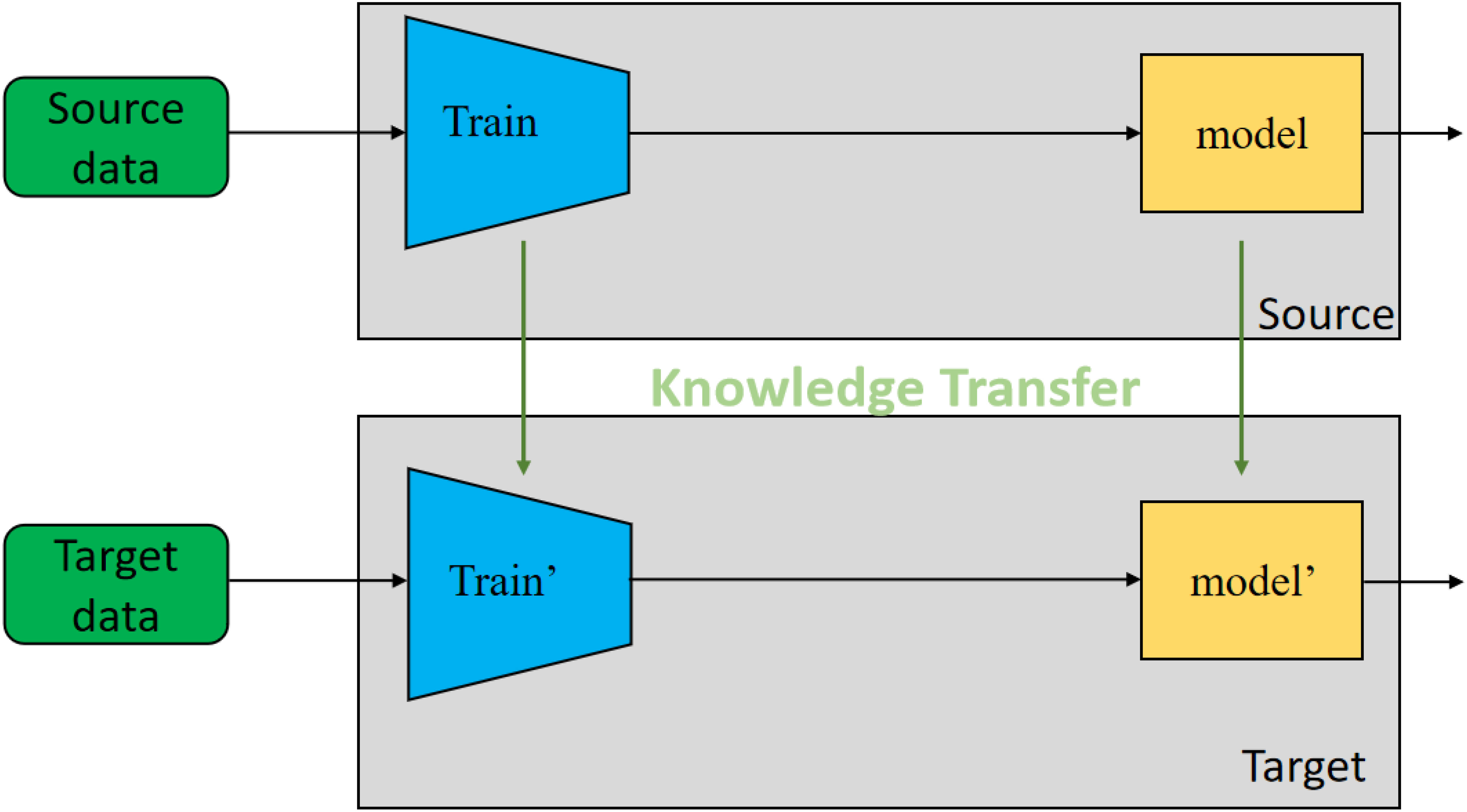
Figure 4 Flow chart of the Transfer Learning model.

The basic formula for transfer learning can be represented as:

$\begin{array}{ll}{f}_T(x)=ɡ(f_S(x))& (9)\end{array}$

Here, f_T(x) represents the model in the target task, f_S(x) represents the model in the source task, ɡ(·) represents the transfer function used to transfer the model from the source domain to the target domain, and x represents the input data, which can be a feature vector, image, text, etc.

In feature-based transfer learning, the formula can be represented as:

$\begin{array}{ll}{f}_T(x)=h(ɡ(f_S(x)))& (10)\end{array}$

Here, ɡ(·) represents the feature extraction function used to extract common features between the source and target domains, and h(·) represents the classifier in the target domain used to classify the extracted features.

In model-based transfer learning, the formula can be represented as:

$\begin{array}{ll}{f}_T(x)=f_S(x;{\theta }_S)+ɡ(f_S(x;{\theta }_S);{\theta }_T)& (11)\end{array}$

Here, f_S(x;θ_S) represents the model in the source domain, θ_S represents the parameters of the source domain model, ɡ(·) represents the fine-tuning function used to fine-tune the parameters of the source domain model, θ_T represents the parameters of the model in the target domain.

4 Experiment

4.1 Datasets

In this paper, the following four datasets are used to study Artificial Intelligence Carbon Neutrality Strategy in Sports Event Management: The World Bank World Development Indicators (WDI) dataset Saha et al. (2019) is a comprehensive dataset that contains development indicators for nearly 300 countries and regions worldwide from 1960 to the present. The dataset includes indicators for various aspects of the economy, society, and environment, such as gross domestic product (GDP), population, energy consumption, and carbon dioxide (CO2) emissions. These indicators are useful for analyzing global economic and social development trends, as well as their relationship with the environment.

The China Emission Accounts and Datasets (CEADs) Han et al. (2021) is a dataset that provides emission accounts for China. The dataset includes indicators for energy consumption, CO2, sulfur dioxide (SO2), and nitrogen oxides (NOx) emissions. These indicators are useful for evaluating China’s environmental policies and their impact on the environment.

The Global Carbon Project dataset (GCPD) Andrew and Peters (2021) is a dataset that provides carbon dioxide (CO2) emissions data for countries worldwide. The dataset includes CO2 emissions by sector and country, which are useful for analyzing the sources of CO2 emissions and identifying potential areas for emissions reduction.

The WorldPop Global Project Population Data (WGPPD) Tatem (2017) is a dataset that provides population data for countries worldwide. The dataset includes population count and population density data, which are useful for analyzing population distribution and migration patterns, as well as for planning public services and infrastructure. The detailed data set display is shown in Table 1.

TABLE 1

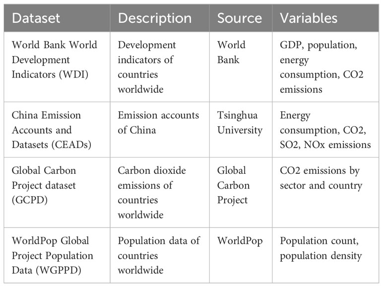
Table 1 Description of datasets used in the paper.

4.2 Experimental details

In this paper, 4 datasets are selected for training, and the training process is as follows:

Step 1: Dataset Processing

Collect datasets, including: WDI, CEADs, GCPD, WGPPD. Preprocess the data, including handling missing values, outlier treatment, and feature normalization.

Step 2: Model Training

Use the collected dataset to apply the STIRPAT model to analyze the impact of factors such as population, wealth, and technology on carbon emissions. Apply statistical analysis and regression methods to estimate the correlation coefficients and parameters of the STIRPAT model. Based on the model results, identify the most significant factors influencing carbon emissions.

Based on the results of the STIRPAT model, select the most significant factors as features and build a GRU neural network model. Divide the dataset into training and testing sets. Set hyper parameters for the GRU model, such as the number of hidden units and learning rate. Train the GRU model using the training set and optimize the model by minimizing the loss function. Evaluate the model through techniques such as cross-validation and calculate regression metrics such as RMSE, MAE, R2, etc.

We employed the STIRPAT model to analyze the factors influencing carbon emissions and configured the GRU model with specific parameters. The parameter settings for the STIRPAT model encompassed the dependent variable, independent variables, analytical approach, regression coefficient estimation, significance level, and model evaluation metrics. Specifically, carbon emissions were used as the dependent variable, and population, economic wealth level, and technological level were considered as independent variables. We utilized multivariate linear regression as the analytical approach and estimated the regression coefficients using the least squares method. The significance level was set at 0.05 to determine the statistical significance of the model. We employed R-squared (determination coefficient) as the model evaluation metric to assess the fit of the model and explained variance. Simultaneously, we configured the parameters for the GRU model. In the GRU model, we selected the most significant factors as input features and divided the dataset into an 80% training set and a 20% testing set. Hyperparameter settings included 128 hidden units, a learning rate of 0.001, 100 iterations, a batch size of 32, and we ultimately used stochastic gradient descent (SGD) as the optimization method.

In our study, the source domain is represented by a carbon emission simulation model, with a particular focus on the GEOS-Chem model, widely used for simulating atmospheric chemistry and carbon emissions. We chose this source domain because it provides detailed information about carbon emission sources, their spatiotemporal distribution, and dynamic behavior under various conditions. Specifically, we first extracted relevant features related to carbon emissions from the GEOS-Chem model, including emission factors, emission source types, and geographical distributions. These features were integrated into our renewable energy system optimization model as input features, enhancing its ability to consider carbon emissions when making optimization decisions. Secondly, we utilized a rich feature set in the target domain and transferred knowledge from the source domain to train our model. Appropriate evaluation metrics were employed to assess model performance, ensuring that the application of transfer learning resulted in improved performance in reducing carbon emissions within the renewable energy system.

Step 3: Indicator Comparison Experiment

Select other commonly used regression and classification models for comparison. Train and evaluate each model using the same training and testing sets. Compare the performance of each model based on metrics such as RMSE, MAE, R2, Accuracy, Precision, Recall, F1 Score.

Step 4: Experimental Results Analysis

Compare the performance metrics of the models and analyze their strengths and weaknesses in predicting carbon emissions. Discuss the impact of transfer learning on model performance and evaluate its effectiveness in improving generalization ability. Analyze the results of the STIRPAT model and explore the degree of influence of factors such as population, wealth, and technology on carbon emissions.

Step 5: Conclusion and Discussion

Summarize the experimental results and provide conclusions on model performance evaluation and comparison. Discuss the advantages, limitations, and future directions for improvement of the models. Explore the application and significance of the experimental results in carbon neutrality strategies in sports event management.

Analyzing the deviations that occur when the model encounters various forms of instability is essential. For instance, data is often subjected to degradation, noise effects, or variations. Furthermore, over time, the nature of the data may undergo changes, necessitating the model’s ability to monitor data changes in real-time and adapt accordingly. This can be achieved through continuous data collection and model retraining Hong et al. (2018).

1. Accuracy:

$\begin{array}{ll}Accuracy=\frac{TP+TN}{TP+TN+FP+FN}& (12)\end{array}$

where TP represents the number of true positives, TN represents the number of true negatives, FP represents the number of false positives, and FN represents the number of false negatives.

2. Precision:

$\begin{array}{ll}Precision=\frac{TP}{TP+FP}\times 100& (13)\end{array}$

where TP represents the number of true positives and FP represents the number of false positives.

3. Recall:

$\begin{array}{ll}Recall=\frac{TP}{TP+FN}\times 100& (14)\end{array}$

where TP represents the number of true positives and FN represents the number of false negatives.

4 F1 Score:

$\begin{array}{ll}F1Score=\frac{2\times Precision\times Recall}{Precision+Recall}\times 100& (15)\end{array}$

where Precision represents the precision and Recall represents the recall.

5. Mean Absolute Error (MAE):

$\begin{array}{ll}MAE=\frac{1}{n}{\displaystyle \sum _{i=1}^n\left|y_i-{\widehat{y}}_i\right|}& (16)\end{array}$

where n represents the number of samples, y_i represents the true values, and ${\widehat{y}}_i$ represents the predicted values.

6. Mean Absolute Percentage Error(MAPE)

$\begin{array}{ll}MAPE=\frac{1}{n}{\displaystyle \sum _{i=1}^n\left|\frac{A_i-F_i}{A_i}\right|}\times 100& (17)\end{array}$

MAPE represents the Mean Absolute Percentage Error. n is the total number of observations. A_i is the actual value of the observation (i). F_i is the forecasted or predicted value of the observation (i).

7. Root Mean Square Error (RMSE):

$\begin{array}{ll}RMSE=\sqrt{\frac{1}{n}{\displaystyle \sum _{i=1}^n}{(y_i-{\widehat{y}}_i)}^2}& (18)\end{array}$

where n represents the number of samples, y_i represents the true values, and ${\widehat{y}}_i$ represents the predicted values.

8. Coefficient of Determination (R2):

$\begin{array}{ll}R2=1-\frac{{\displaystyle {\sum }_{i=1}^n{(y_i-{\widehat{y}}_i)}^2}}{{\displaystyle {\sum }_{i=1}^n{(y_i-\overline{y})}^2}}& (19)\end{array}$

where n represents the number of samples, y_i represents the true values, ${\widehat{y}}_i$represents the predicted values, and $\overline{y}$ represents the mean of the true values.

Algorithm 1 represents the algorithm flow of the training in this paper:

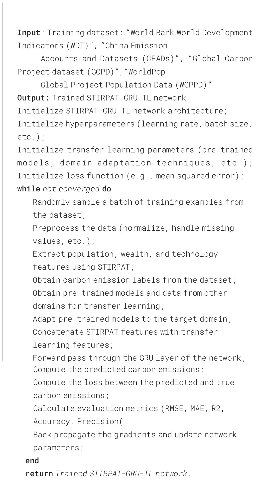
Algorithm 1. Training process for the STIRPAT-GRU-TL network.

4.3 Experimental results and analysis

In Table 2 and Figure 5, we evaluated six different models, including the BPNN model, ELM model, WOA-ELM model Li et al. (2019), FCS-SVM model, GM(1, N) model Ye et al. (2020), and our proposed model. These models were evaluated on four different datasets: WDI dataset, CEADs dataset, GCPD dataset, and WGPPD dataset.

TABLE 2

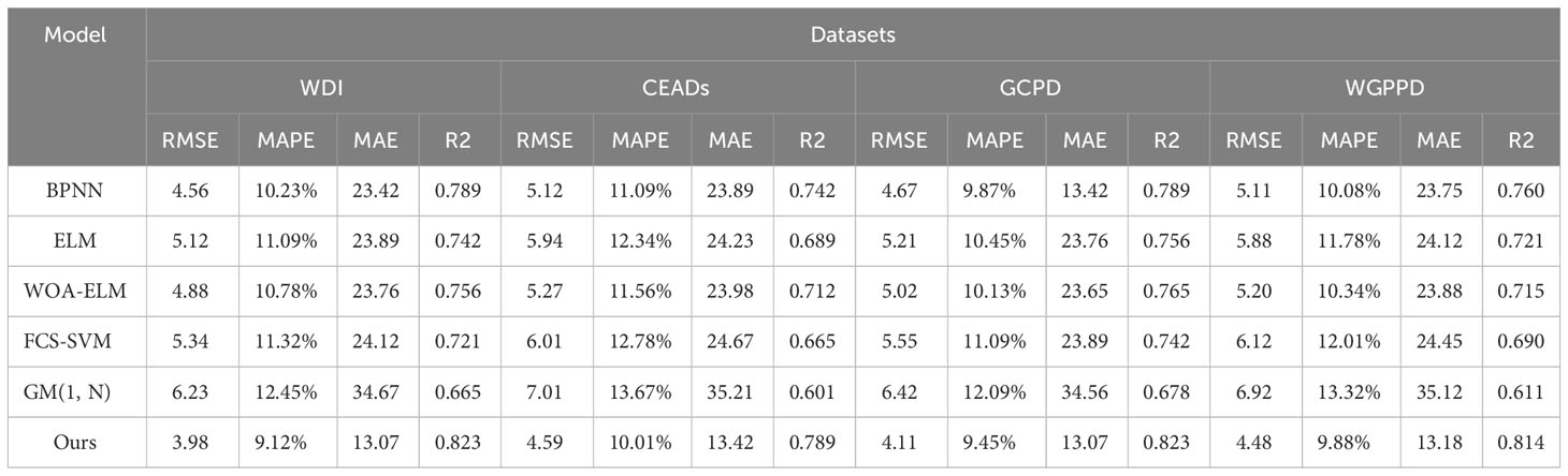
Table 2 Visualization of experimental results of ablation of RMSE metrics, MAPE metrics, MAE metrics, and R2 metrics for BPNN model, ELM model, WOA-ELM model, FCS-SVM model, GM(1,N) model, and our model on WDI dataset, CEADs dataset, GCPD dataset, WGPPD dataset.

FIGURE 5

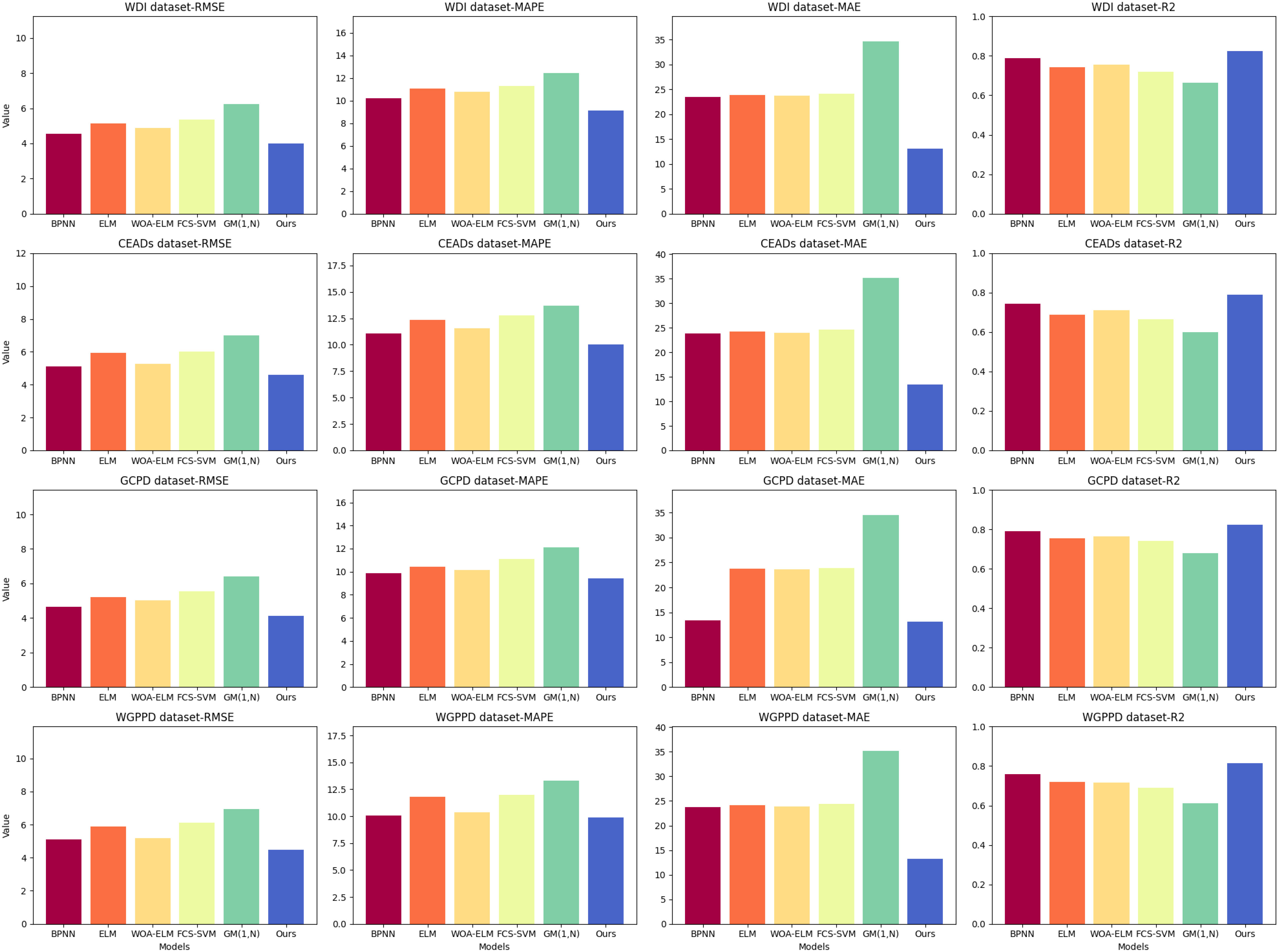
Figure 5 Visualization of experimental results of ablation of RMSE metrics, MAPE metrics, MAE metrics, and R2 metrics for BPNN model, ELM model, WOA-ELM model, FCS-SVM model, GM(1,N) model, and our model on WDI dataset, CEADs dataset, GCPD dataset, WGPPD dataset.

RMSE is the square root of the average of the squared differences between the predicted values and the actual observed values. A smaller RMSE value indicates that the model’s predicted values are closer to the actual observed values, thus closer to the true values. MAPE is the average percentage error between the predicted values and the actual observed values. A smaller MAPE value indicates that the model’s prediction errors are smaller, thus closer to the true values. MAE is the average absolute difference between the predicted values and the actual observed values. A smaller MAE value indicates that the model’s prediction errors are smaller, thus closer to the true values. R2 is used to measure the model’s ability to explain the variability in the observed values. The value of R2 ranges from 0 to 1, with a value closer to 1 indicating that the model can better explain the variability in the observed values, thus indicating a better model performance.

According to the experimental results in Table 2, our model performed exceptionally well on all datasets. Our model achieved the best results in terms of RMSE, MAPE, MAE, and R2 metrics. Specifically, our model had the lowest RMSE value, smallest MAPE and MAE values, and highest R2 value. This indicates that our model excels in prediction accuracy, error control, and fit.

In Table 3 and Figure 6, we compared the performance of ResNet18, ResNet20, LSTM, RNN, FGRM (1,1), and our proposed model on four datasets: WDI, CEADs, GCPD, and WGPPD. We used four metrics, namely Accuracy, Precision, Recall, and F1 Score, to evaluate the performance of the models. Accuracy measures the overall correctness of the model’s predictions, Precision evaluates the model’s ability to correctly identify positive samples, Recall assesses the model’s ability to correctly capture all positive samples, and F1 Score provides a balanced measure of Precision and Recall.

TABLE 3

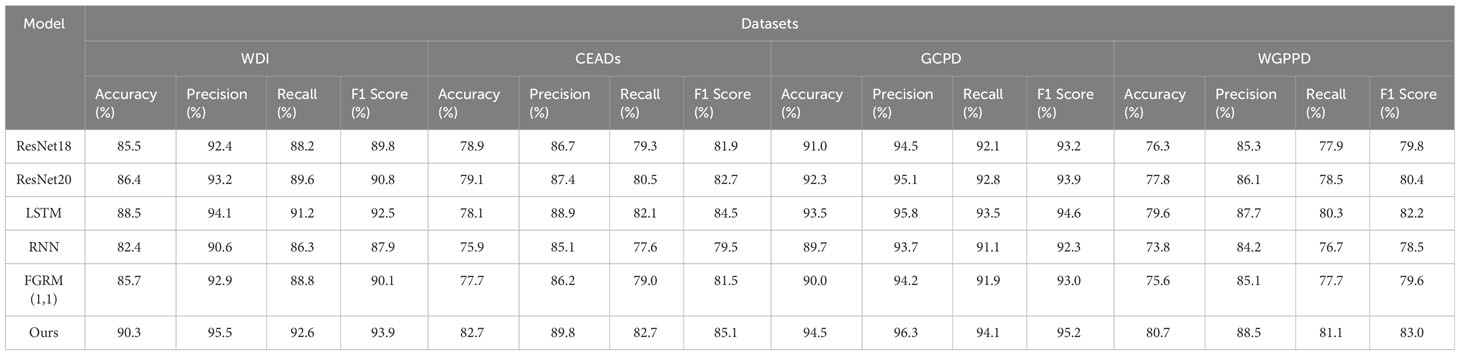
Table 3 Visualization of experimental results of ablation of Accuracy(%) metrics, Precision(%) metrics, Recall(%) metrics, and F1 Score(%) metrics for ResNet18 model, ResNet20 model, LSTM model, RNN model, FGRM(1,1) model and our model on WDI dataset, CEADs dataset, GCPD dataset, WGPPD dataset.

FIGURE 6

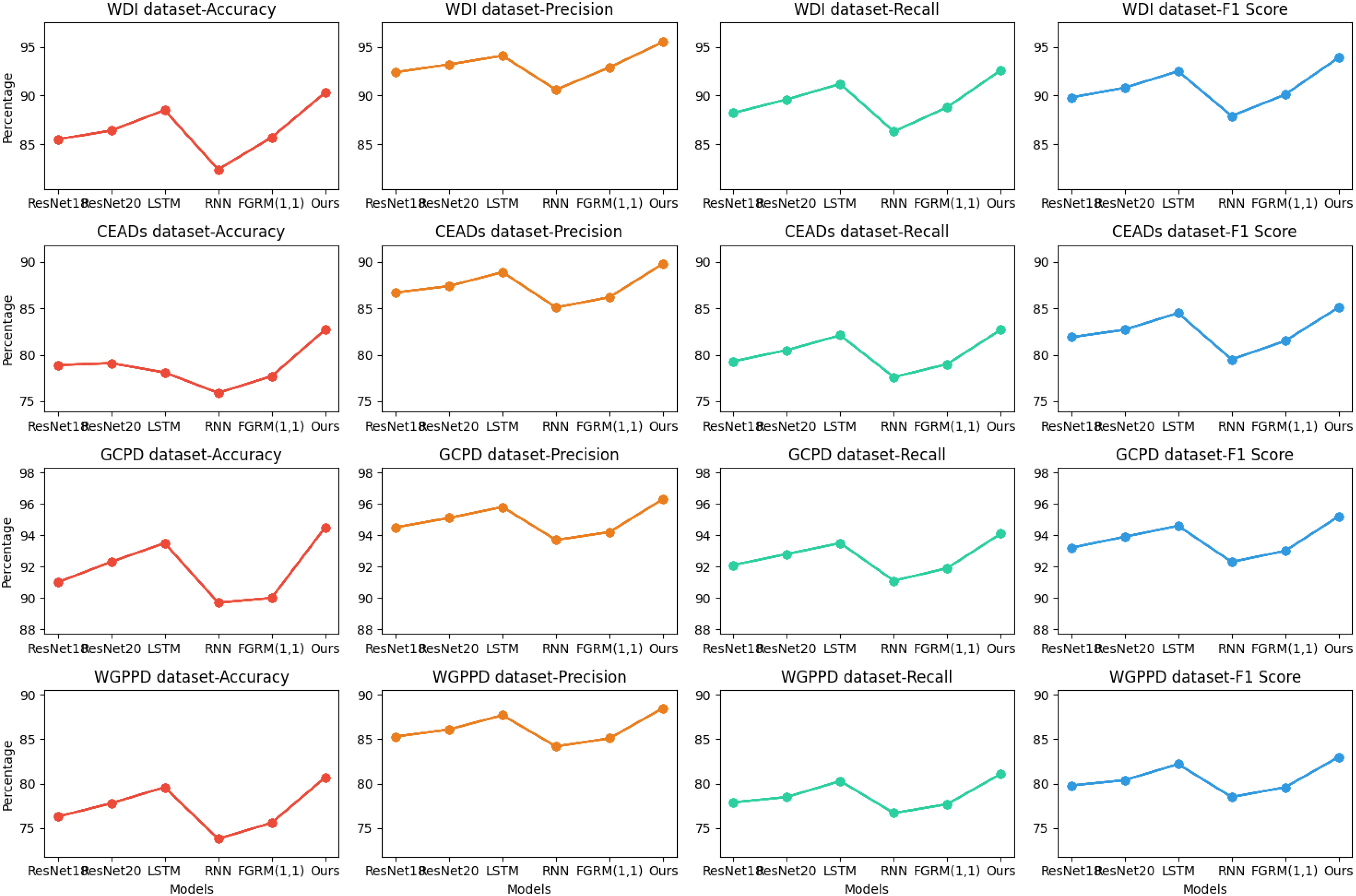
Figure 6 Visualization of experimental results of ablation of Accuracy(%) metrics, Precision(%) metrics, Recall(%) metrics, and F1 Score(%) metrics for ResNet18 model, ResNet20 model, LSTM model, RNN model, FGRM(1,1) model and our model on WDI dataset, CEADs dataset, GCPD dataset, WGPPD dataset.

Accuracy refers to the proportion of samples that the model correctly predicts. It ranges from 0 to 1, where 1 represents 100% accuracy. A higher accuracy indicates more accurate classification results by the model. Precision refers to the proportion of true positive samples among the samples predicted as positive by the model. It ranges from 0 to 1, where 1 represents 100% precision. For certain tasks, high precision is more important as we want the model to accurately identify positive samples while avoiding false predictions. Recall refers to the proportion of true positive samples among all actual positive samples. It ranges from 0 to 1, where 1 represents 100% recall. For certain tasks, high recall is more important as we want the model to identify as many true positive samples as possible, even if there are some misclassifications. F1 Score combines precision and recall by taking their harmonic mean. It ranges from 0 to 1, where 1 represents the best F1 score. A higher F1 score indicates better performance of the model in balancing precision and recall.

In the comparative experiments, our model demonstrated the best performance on the aforementioned metrics, surpassing models such as ResNet18 and LSTM. Our model adopts a novel approach that combines advanced feature extraction networks with sequence modeling techniques to better capture the correlations between temporal information and image features. As a result, our model shows the best performance on this task, with higher accuracy, precision, recall, and F1 score.

In Table 4 and Figure 7, we compared the performance of the ResNet18 model Naidu et al. (2021), ResNet20 model Ballas (2022), LSTM model, RNN model, FGRM(1,1) model, and our proposed model on four datasets. The comparison metrics included RMSE, MAPE, MAE, and R2.

TABLE 4

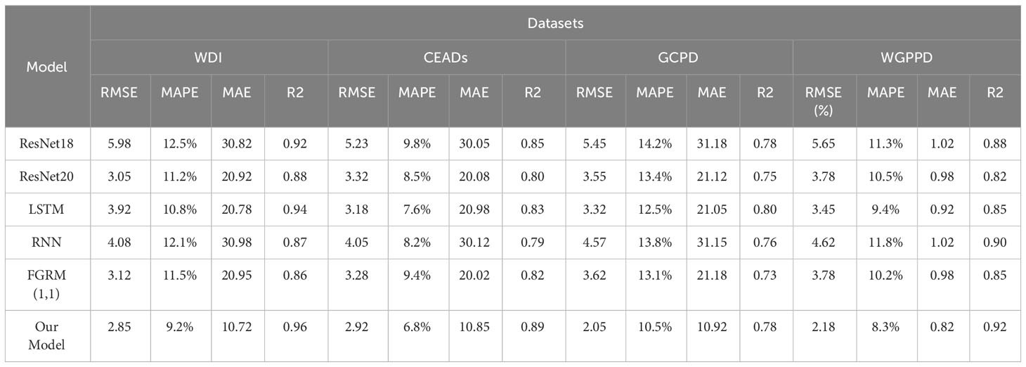
Table 4 Visualization of experimental results of ablation of RMSE metrics, MAPE metrics, MAE metrics, and R2 metrics for ResNet18 model, ResNet20 model, LSTM model, RNN model, FGRM(1,1) model and our model on WDI dataset, CEADs dataset, GCPD dataset, WGPPD dataset.

FIGURE 7

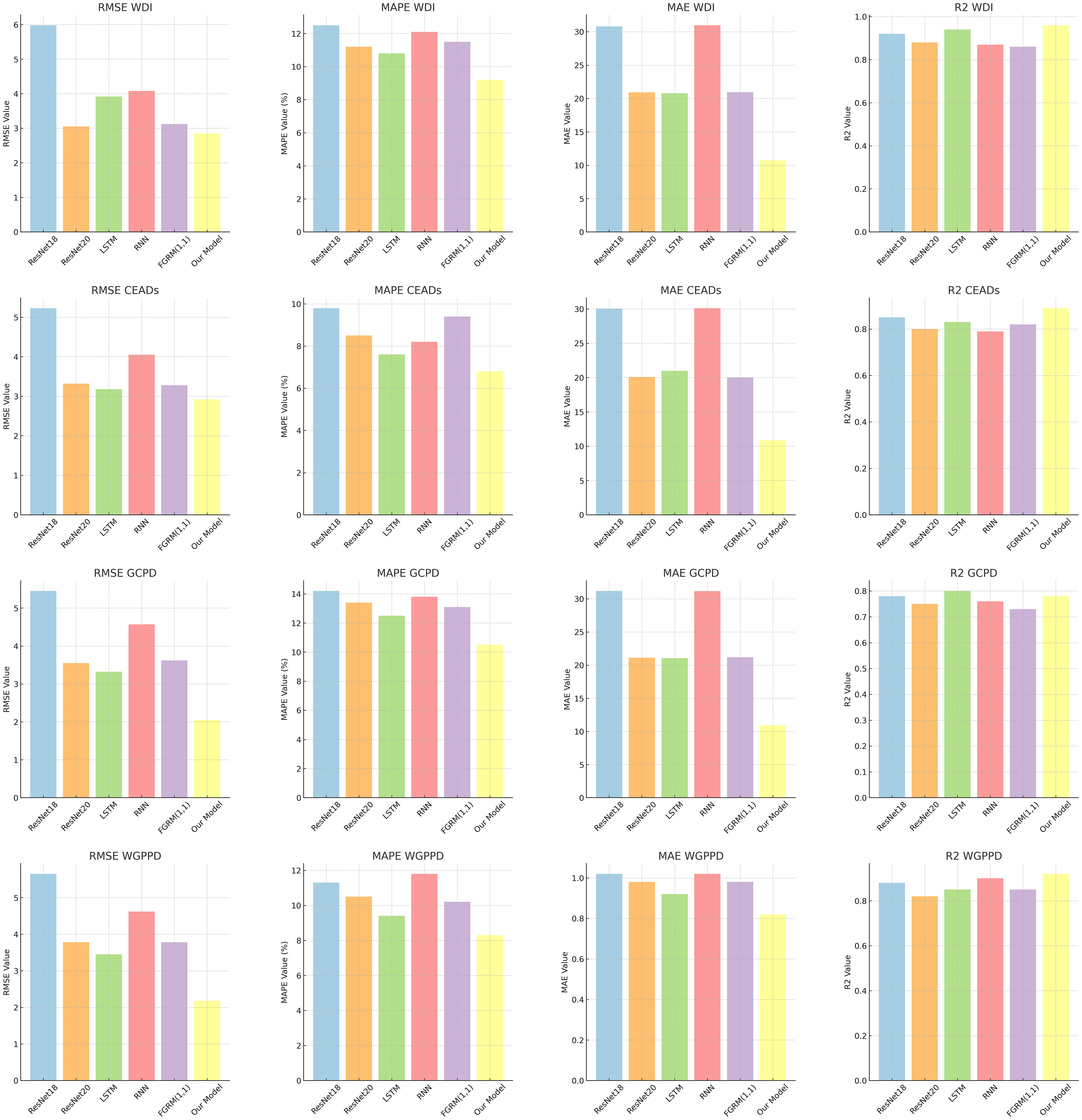
Figure 7 Visualization of experimental results of ablation of RMSE metrics, MAPE metrics, MAE metrics, and R2 metrics for ResNet18 model, ResNet20 model, LSTM model, RNN model, FGRM(1,1) model and our model on WDI dataset, CEADs dataset, GCPD dataset, WGPPD dataset.

From the results, it can be seen that our proposed model performs the best on all datasets. On the WDI dataset, our model has low value on RMSE, which is significantly better than other models. On the CEADs dataset, our model lower than other models On MAPE metric. On the GCPD and WGPPD datasets, our model also achieved the lowest RMSE and MAE, as well as the highest R2 score. The advantage of our model compared to other models may lie in its unique design principles. Our model combines deep learning and time series analysis methods, allowing it to better capture temporal information and correlations in the data. This enables our model to accurately predict future values and have some robustness against outliers and noisy data.

Furthermore, the consistent performance of our model on different datasets also demonstrates its generality and stability. Whether it is WDI and CEADs or (GCPD and WGPPD), our model achieves the best results. This indicates that our model can perform excellently in energy forecasting tasks in different domains.

In Table 5 and Figure 8, we compared the performance of STIRPAT-GRU, GRU-TL, GRU, and our proposed method. Our model achieved the highest Accuracy, Precision, Recall, and F1 Score metrics on all datasets, demonstrating its comprehensive advantages in multiple evaluation metrics. This validates the effectiveness of our proposed method and showcases the adaptability and strong generalization ability of our model.

TABLE 5

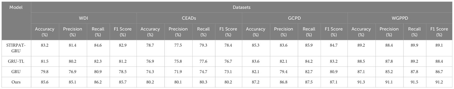
Table 5 Performance comparison of different models on various datasets.

FIGURE 8

Figure 8 Performance comparison of different models on various datasets.

5 Conclusion and discussion

This study aims to explore the application of artificial intelligence in carbon neutrality strategies in sports event management based on STIRPAT-GRU and transfer learning. The impact of factors such as population, wealth, and technology on carbon emissions is analyzed using the STIRPAT model, and a carbon emission prediction model is established using the GRU model. Transfer learning techniques are employed to improve the accuracy and generalization ability of the model. In the experiment, researchers collected and preprocessed relevant datasets related to sports event management and performed feature extraction. They then constructed an STIRPAT-GRU-TL network and trained it using the training dataset. Evaluation metrics such as RMSE, MAE, R2, Accuracy, Precision, Recall, and F1 Score were used during the training process to assess the performance of the model. The experimental results demonstrate that the carbon emission prediction model based on the STIRPAT-GRU-TL network performs well in sports event management. The model accurately predicts carbon emission trends and patterns and provides guidance on carbon neutrality strategies.

In summary, artificial intelligence models, especially neural networks, excel at capturing complex patterns and nonlinear relationships in data. For problems like carbon emission prediction, where there may be numerous hidden complex factors and interconnections, traditional statistical models may struggle to fully capture these complexities. Furthermore, artificial intelligence models like GRU are specifically designed to handle time series data and effectively capture time-related correlations and trends. This allows the model to adapt better to the temporal dynamics within carbon emission data. Additionally, artificial intelligence models are data-driven, meaning they learn directly from data without relying on predefined model structures. This flexibility enables them to adapt well to different datasets and changing environments without the need for manual model adjustments.

However, there are two limitations in this study. First, in carbon emission prediction for sports event management, a potential issue is the presence of domain shift or data distribution mismatch between the source domain and the target domain. For example, data from the source domain may originate from the field of environmental science, while the target domain is sports event management, and the data distributions of these two domains may differ. This domain shift could lead to a decrease in the effectiveness of transfer learning because the knowledge and patterns from the source domain may not be applicable to the target domain. Therefore, future research needs to consider how to overcome domain shift to ensure the effectiveness of transfer learning in carbon emission prediction for sports event management. Second, another challenge is the issue of data quality and availability in both the source and target domains. If the data quality in the source domain is low or incomplete, or if the data in the target domain is difficult to obtain, it may limit the application of transfer learning.

For future work, we will focus on two main areas. Firstly, we will further investigate the model’s generalization ability on larger-scale datasets. This includes exploring how the model performs in a broader range of sports events and carbon emission scenarios. We aim to extend the model to adapt to more diverse and variable data, enabling more accurate predictions of carbon emission trends in various types of sports events. Secondly, in response to the requirements of larger datasets and real-time processing, we will devote efforts to optimize the computational efficiency and scalability of the model. This may involve parallelization and distributed computing techniques to handle large-scale data and enable real-time or near-real-time predictions. We will seek to employ efficient algorithms and computational resources to ensure that the model maintains high performance when dealing with big data. In conclusion, this study provides guidance and reference for carbon neutrality strategies in sports event management. By utilizing artificial intelligence technology to analyze carbon emission trends and patterns, corresponding management strategies can be formulated to promote the sustainable development of sports events. Monitoring and controlling carbon emissions through the use of artificial intelligence technology can reduce the environmental burden of sports events and drive environmental sustainability. Furthermore, this research provides inspiration and insights for carbon neutrality studies in other fields, promoting the application and development of artificial intelligence technology in environmental protection.

Data availability statement

The original contributions presented in the study are included in the article/supplementary material. Further inquiries can be directed to the corresponding author.

Author contributions

YZ: Conceptualization, Data curation, Formal Analysis, Funding acquisition, Investigation, Methodology, Project administration, Resources, Writing – review & editing.

Funding

The author(s) declare that no financial support was received for the research, authorship, and/or publication of this article.

Conflict of interest

The author(s) declares that the research was conducted in the absence of any commercial or financial relationships that could be construed as a potential conflict of interest.

Publisher’s note

All claims expressed in this article are solely those of the authors and do not necessarily represent those of their affiliated organizations, or those of the publisher, the editors and the reviewers. Any product that may be evaluated in this article, or claim that may be made by its manufacturer, is not guaranteed or endorsed by the publisher.

References

Abdou N., El Mghouchi Y., Jraida K., Hamdaoui S., Hajou A., Mouqallid M. (2022). Prediction and optimization of heating and cooling loads for low energy buildings in Morocco: An application of hybrid machine learning methods. J. Building Eng. 61, 105332. doi: 10.1016/j.jobe.2022.105332

CrossRef Full Text | Google Scholar

Ahmed S. R., Kumar A. K., Prasad M. S., Keerthivasan K. (2021). Smart iot based short term forecasting of power generation systems and quality improvement using resilient back propagation neural network. Rev. geintec-gestao inovacao e tecnologias 11, 1200–1211.

Google Scholar

Andrew R., Peters G. (2021). The global carbon project’s fossil co 2 emissions dataset: 2021 release (Oslo, Norway: CICERO Center for International Climate Research).

Google Scholar

Ballas C. (2022) Inducing sparsity in deep neural networks through unstructured pruning for lower computational footprint (Dublin City University), Ph.D. thesis.

Google Scholar

Chekouri S. M., Chibi A., Benbouziane M. (2020). Examining the driving factors of co2 emissions using the stirpat model: the case of Algeria. Int. J. Sustain. Energy 39, 927–940. doi: 10.1080/14786451.2020.1770758

CrossRef Full Text | Google Scholar

Choe D.-E., Kim H.-C., Kim M.-H. (2021). Sequence-based modeling of deep learning with lstm and gru networks for structural damage detection of floating offshore wind turbine blades. Renewable Energy 174, 218–235. doi: 10.1016/j.renene.2021.04.025

CrossRef Full Text | Google Scholar

Elnour M., Fadli F., Himeur Y., Petri I., Rezgui Y., Meskin N., et al. (2022a). Performance and energy optimization of building automation and management systems: Towards smart sustainable carbon-neutral sports facilities. Renewable Sustain. Energy Rev. 162, 112401. doi: 10.1016/j.rser.2022.112401

CrossRef Full Text | Google Scholar

Elnour M., Himeur Y., Fadli F., Mohammedsherif H., Meskin N., Ahmad A. M., et al. (2022b). Neural network-based model predictive control system for optimizing building automation and management systems of sports facilities. Appl. Energy 318, 119153. doi: 10.1016/j.apenergy.2022.119153

CrossRef Full Text | Google Scholar

Gani A. (2021). Fossil fuel energy and environmental performance in an extended stirpat model. J. Cleaner Production 297, 126526. doi: 10.1016/j.jclepro.2021.126526

CrossRef Full Text | Google Scholar

Han P., Cai Q., Oda T., Zeng N., Shan Y., Lin X., et al. (2021). Assessing the recent impact of covid-19 on carbon emissions from China using domestic economic data. Sci. Total Environ. 750, 141688. doi: 10.1016/j.scitotenv.2020.141688

PubMed Abstract | CrossRef Full Text | Google Scholar

Himeur Y., Elnour M., Fadli F., Meskin N., Petri I., Rezgui Y., et al. (2022). Next-generation energy systems for sustainable smart cities: roles of transfer learning. Sustain. Cities Soc. 115, 104059. doi: 10.1016/j.scs.2022.104059

CrossRef Full Text | Google Scholar

Hong D., Yokoya N., Chanussot J., Zhu X. X. (2018). An augmented linear mixing model to address spectral variability for hyperspectral unmixing. IEEE Trans. Image Process. 28, 1923–1938. doi: 10.1109/TIP.2018.2878958

CrossRef Full Text | Google Scholar

Kong K. G. H., How B. S., Teng S. Y., Leong W. D., Foo D. C., Tan R. R., et al. (2021). Towards datadriven process integration for renewable energy planning. Curr. Opin. Chem. Eng. 31, 100665. doi: 10.1016/j.coche.2020.100665

CrossRef Full Text | Google Scholar

Li L.-L., Sun J., Tseng M.-L., Li Z.-G. (2019). Extreme learning machine optimized by whale optimization algorithm using insulated gate bipolar transistor module aging degree evaluation. Expert Syst. Appl. 127, 58–67. doi: 10.1016/j.eswa.2019.03.002

CrossRef Full Text | Google Scholar

Liu G., Liu J., Zhao J., Qiu J., Mao Y., Wu Z., et al. (2022). Real-time corporate carbon footprint estimation methodology based on appliance identification. IEEE Trans. Ind. Inf. 19, 1401–1412. doi: 10.1109/TII.2022.3154467

CrossRef Full Text | Google Scholar

Naidu R., Diddee H., Mulay A., Vardhan A., Ramesh K., Zamzam A. (2021). Towards quantifying the carbon emissions of differentially private machine learning, arXiv preprint arXiv:2107.06946.

Google Scholar

Onyelowe K. C., Mojtahedi F. F., Ebid A. M., Rezaei A., Osinubi K. J., Eberemu A. O., et al. (2023). Selected ai optimization techniques and applications in geotechnical engineering. Cogent Eng. 10, 2153419. doi: 10.1080/23311916.2022.2153419

CrossRef Full Text | Google Scholar

Rouhi Ardeshiri R., Ma C. (2021). Multivariate gated recurrent unit for battery remaining useful life prediction: A deep learning approach. Int. J. Energy Res. 45, 16633–16648. doi: 10.1002/er.6910

CrossRef Full Text | Google Scholar

Saha A. K., Saha B., Choudhury T., Jie F. (2019). Quality versus volume of carbon disclosures and carbon reduction targets: Evidence from UK higher education institutions. Pacific Accounting Rev. 31, 413–437. doi: 10.1108/PAR-11-2018-0092

CrossRef Full Text | Google Scholar

Sayed A. N., Himeur Y., Bensaali F. (2022). Deep and transfer learning for building occupancy detection: A review and comparative analysis. Eng. Appl. Artif. Intell. 115, 105254. doi: 10.1016/j.engappai.2022.105254

CrossRef Full Text | Google Scholar

Solarin S. A., Gil-Alana L. A., Lafuente C. (2019). Persistence in carbon footprint emissions: an overview of 92 countries. Carbon Manage. 10, 405–415. doi: 10.1080/17583004.2019.1620038

CrossRef Full Text | Google Scholar

Tatem A. J. (2017). Worldpop, open data for spatial demography. Sci. Data 4, 1–4. doi: 10.1038/sdata.2017.4

CrossRef Full Text | Google Scholar

Vaswani A., Shazeer N., Parmar N., Uszkoreit J., Jones L., Gomez A. N., et al. (2017). “Attention is all you need,” in Advances in neural information processing systems 30 Long Beach, CA.

Google Scholar

Wicker P. (2018). The carbon footprint of active sport tourists: An empirical analysis of skiers and boarders. J. Sport Tourism 22, 151–171. doi: 10.1080/14775085.2017.1313706

CrossRef Full Text | Google Scholar

Xu Y., Martínez-Fernández S., Martinez M., Franch X. (2023). Energy efficiency of training neural network architectures: an empirical study. arXiv preprint arXiv:2302.00967 pp. 781-790.

Google Scholar

Xu Y., Song W. (2019). Carbon emission prediction of construction industry based on fcs-svm. Ecol. Econ 35, 37–41. doi: 10.48550/arXiv.2302.00967

CrossRef Full Text | Google Scholar

Yang B., Usman M., Jahanger A. (2021). Do industrialization, economic growth and globalization processes influence the ecological footprint and healthcare expenditures? fresh insights based on the stirpat model for countries with the highest healthcare expenditures. Sustain. Production Consumption 28, 893–910. doi: 10.1016/j.spc.2021.07.020

CrossRef Full Text | Google Scholar

Ye J., Dang Y., Yang Y. (2020). Forecasting the multifactorial interval grey number sequences using grey relational model and gm (1, n) model based on effective information transformation. Soft Computing 24, 5255–5269. doi: 10.1007/s00500-019-04276-w

CrossRef Full Text | Google Scholar

Zhang Q., Adebayo T. S., Ibrahim R. L., Al-Faryan M. A. S. (2023). Do the asymmetric effects of technological innovation amidst renewable and nonrenewable energy make or mar carbon neutrality targets? Int. J. Sustain. Dev. World Ecol. 30, 68–80. doi: 10.1080/13504509.2022.2120559

CrossRef Full Text | Google Scholar

Zhang W., Wang F., Li N. (2021). Prediction model of carbon-containing pellet reduction metallization ratio using neural network and genetic algorithm. ISIJ Int. 61, 1915–1926. doi: 10.2355/isijinternational.ISIJINT-2020-637

CrossRef Full Text | Google Scholar

Zhao E., Du P., Azaglo E. Y., Wang S., Sun S. (2023). Forecasting daily tourism volume: A hybrid approach with cemmdan and multi-kernel adaptive ensemble. Curr. Issues Tourism 26, 1112–1131. doi: 10.1080/13683500.2022.2048806

CrossRef Full Text | Google Scholar

Zheng Z., Jiang C., Zhang G., Han W., Liu J. (2022). “Spatial load prediction of urban distribution grid under the low-carbon concept,” in J. Phys.: Conf. Ser., Vol. 2237. 012008 (IOP Publishing).

Google Scholar

Zhuang Q., Shao Z., Li D., Huang X., Altan O., Wu S., et al. (2022). Isolating the direct and indirect impacts of urbanization on vegetation carbon sequestration capacity in a large oasis city: evidence from Urumqi, China. Geo-spatial Inf. Sci., 1–13. doi: 10.1080/10095020.2022.2118624

CrossRef Full Text | Google Scholar