Detecting and monitoring rodents using camera traps and machine learning versus live trapping for occupancy modeling

1 Introduction

Loss of biodiversity is a global problem occurring across wildlife communities (Worm et al., 2006; Barnosky et al., 2011; Cardinale et al., 2012; McCallum, 2015), with growing evidence indicating a sixth mass extinction is underway (Dirzo et al., 2014; Ceballos et al., 2015). The current rate of extinctions, and loss of biodiversity, is arguably one of the biggest environmental issues today, both for the health of ecosystems, and the health of humans (Ceballos et al., 2015). In the United States of America, over 1500 species are listed as threatened or endangered under the Endangered Species Act (ESA) (U.S. Fish Wildlife Service, 2022), requiring recovery plans for each listing. These recovery plans identify threats to species and management priorities, among other things (Schwartz, 2008). Therefore, detailed knowledge of the species’ ecology and interactions with its habitat is required. Yet by the time species are listed as endangered and the need for conservation attention is recognized, population sizes and limited remaining habitat make inference and recovery problematic (Schwartz, 2008). This makes monitoring both necessary, and simultaneously more difficult, for rare species.

Efficient and effective methods to detect (determine or confirm presence) and monitor populations would be one way to support conservation and wildlife management during this time of extreme species loss and anthropogenic disturbance. The best methods to detect and monitor populations balance effort and efficiency without sacrificing the quality data required for successful management and conservation. Monitoring changes in detection and in species occurrence (which areas are occupied) while exploring habitat associations is an effective way to gather information for successful management (Diggins et al., 2016) and can be done through occupancy models (MacKenzie et al., 2002).

Presence/absence data collected through various techniques can be used to estimate a detection probability and an occupancy estimate for species (MacKenzie et al., 2002). Detection probability is how likely the species is actually detected should it be present. Occupancy is the proportion of sample units occupied by a species, and subsequently occupancy estimate, or occupancy probability, is the probability that sampling units are occupied by a species when detection probability is considered (MacKenzie et al., 2017). The detectability of a species can be influenced by numerous factors (abundance, behavior, survey effort, etc.) (Welsh et al., 2013; Guillera-Arroita, 2017) and different techniques used to collect the data may vary in detection probability (Bailey et al., 2004; O’Connell et al., 2006; Guillera-Arroita, 2017). When trying to detect rare or cryptic species, techniques that provide the highest probabilities of detection need to be used to ensure the best chance of detecting the species should it be present.

Different species can have different detection probabilities, but different detection techniques may exacerbate heterogeneity in detection. Heterogeneity is when different individuals or categories of individuals within a species have different (heterogeneous) detection probabilities. If the cause of heterogeneity in detection cannot be modeled or is unknown, occupancy estimates will be biased (MacKenzie et al., 2017). Therefore, using detection methods with fewer suspected possible sources of heterogeneity in detection should lead to more accurate occupancy estimates. Likewise, using the detection method with the greatest mean detection probability may make detection heterogeneity insignificant (MacKenzie et al., 2017). Importantly, occupancy models can be used not only to evaluate habitat attributes and management actions, but also to compare the probability of detection across monitoring methods themselves. Therefore, we wanted to explore the outcome of different monitoring methods on detection and occupancy estimates to determine which is best at detecting species and best at providing accurate estimates of occupancy probabilities.

We focus on small mammal monitoring methods, specifically for rodents (order Rodentia). Rodents are an abundant and highly diverse taxonomic group, making up 39% of all mammal species (Burgin et al., 2018). There are currently 332 rodent species listed as threatened on the IUCN red list (IUCN, 2022). Given the vital importance of rodents for ecosystem health (Avenant, 2011) and the vast number of threatened species, determining the most effective monitoring techniques might allow for practical and reasonable solutions to monitoring and detection that could assist conservation efforts and land managers. Additionally, effective detection could inform invasive rodent management where detection and monitoring are critical to assessing management success, maintaining biosecurity, or providing safeguards to sensitive species or ecosystems.

Live trapping is commonly used for monitoring small mammals (Tasker and Dickman, 2001; Baker et al., 2003; Flowerdew et al., 2004). Live trapping allows the collection of data on individuals: species, sex, reproductive condition, and age. It allows individuals to be uniquely marked for mark-recapture analyses that can answer demographic questions about abundance, survival, and movement (Patterson et al., 1989; Lettink and Armstrong, 2003). Live trapping can also provide presence/absence data for use in occupancy models to understand how occurrence varies with site attributes (Walpole and Bowman, 2011; Santulli et al., 2014; Tobin et al., 2014). However, rodent detection through live traps could be influenced by trap saturation (i.e., traps not available for capture of an individual due to it already being occupied), odors (Boonstra and Krebs, 1976; Mazdzer et al., 1976; Daly et al., 1978; Daly et al., 1980), individual behavior (Tanaka, 1963; Gurnell, 1972; Gurnell, 1982), and species behavior (Gurnell, 1982; Stokes, 2012). Therefore, live traps could confer low detection probability and/or possible sources of detection heterogeneity that may influence occupancy estimates. Live trapping requires rodent entrapment (for 8+ hours depending on season) and direct handling of wildlife, possibly inducing stress responses or mortality in captured individuals (Fletcher and Boonstra, 2006; Delehanty and Boonstra, 2009), and injury or disease transmission to handlers. Additionally, live trapping can require substantial field effort and training. Traps must be set and checked each day (or more often for listed species), requiring multiple visits per day to the study site and time for processing animals prior to release. Increasing effort by trapping for more nights or by using more traps per trap station would increase detection (Hice and Velazco, 2013), but the need to entrap would maintain sources of heterogeneity. While effort itself may be constrained by resources available to a monitoring program. Therefore, live traps may be an inefficient method of small mammal monitoring, compared to other methods, due to detection, analysis, welfare, and effort.

Camera trapping is another method commonly used for monitoring mammals (Yasuda, 2004; Tobler et al., 2008; Pettorelli et al., 2010). Cameras can be used to collect presence/absence data, and data for demographic analyses if individuals are uniquely identifiable through images (Carbone et al., 2001), though rodents do not typically display obvious physical differences across individuals. Instead, presence/absence data sets of rodents for occupancy modeling can be produced with relatively small field effort since cameras do not need to be checked daily. Cameras provide a noninvasive way to monitor without direct handling and entrapment stress, greater detection for cryptic or trap-shy species (Claridge et al., 2004; Gray et al., 2017), and unlimited detections (i.e., no trap saturation). These characteristics may confer greater mean detection probability compared to live traps, possibly increasing the detection of rare species and reducing sources of detection heterogeneity, providing more accurate estimates of occupancy probability.

Multiple rodent species with similar physical characteristics are often found in a single community. Therefore, researchers must be able to correctly identify different species within the camera images for camera trapping to be a valid monitoring technique. Meek et al. (2013) argued that cameras make the correct identification of small mammal species with similar physical characteristics problematic. However, De Bondi et al. (2010) and Gray et al. (2017) have shown that mounting cameras horizontally with the lens facing the ground allows a view of the dorsum, and facilitates correct identification of small mammals, thus providing reliable (Gray et al., 2017; Thomas et al., 2019) presence/absence data.

A remaining drawback to cameras is the huge number of images that are produced. One camera in the field for one night could capture as many as 5,000 images, or over 1.8 million in a single year, depending on the setting used and activity detected. While live trapping requires greater field effort compared to camera traps, the lab effort required to process camera images can make total effort across the two methods comparable (Diggins et al., 2016).

We examined the effectiveness of the two common monitoring methods, live traps and camera traps, for both detecting and analyzing occupancy probabilities specifically in six species of rodents. We explored an artificial intelligence (AI) model to reduce effort and provide an efficient and manageable way to process rodent camera trap images, by developing and assessing a machine learning (ML) model to process our images. ML models have shown success in processing camera images for various taxa (Tabak et al., 2019; Tabak et al., 2020; Whytock et al., 2021). It is possible that with the use of new technology to improve camera image processing, camera trapping might require lower monitoring effort compared to live trapping while resulting in higher detection probability for rodent species.

Recent advances in machine learning (ML), specifically convolutional neural networks (CNNs), offer promising, potentially cost-effective, solutions to camera trap image processing (Norouzzadeh et al., 2017; Tabak et al., 2019; Willi et al., 2019). Within vertebrates, CNNs have been tested for identification of medium to large mammal and fish species (Norouzzadeh et al., 2017; Villa et al., 2017; Villon et al., 2018; Schneider et al., 2019), and it has been shown that CNNs correctly identify these species and greatly reduce the image processing effort (Norouzzadeh et al., 2017; Villa et al., 2017; Villon et al., 2018; Schneider et al., 2019). A recent study used a CNN model to successfully identify four rodent species, with images collected in the traditional vertical camera placement (Seijas et al., 2019). However, to our knowledge ML with CNNs has not been tested on species-level identification in a community of six rodents and with a dorsal view.

For this comparison of live traps versus camera traps at both detecting and analyzing occupancy, we formed three predictions. We hypothesized that detection probability would significantly vary across baited live traps and baited camera traps. We predicted camera traps would yield greater detection probabilities for all species. We hypothesized that occupancy estimates would also vary across the two detection methods since we hypothesized different detection probabilities from each method. We predicted that baited camera traps would yield higher occupancy estimates due to greater detection. We also predicted that, while occupancy estimates would vary across the two methods, qualitatively, the influence of habitat attributes on occupancy estimates would be the same regardless of method. Additionally, we hypothesized that using ML via CNNs would change the effort associated with camera trapping, and predicted camera trapping effort could be reduced making monitoring more practical and accessible for land managers.

2 Materials and methods

2.1 Study site

To compare the two monitoring methods, six rodent species were trapped at Oceano Dunes State Vehicle Recreation Area (ODSVRA) in San Luis Obispo County, California, U.S.A. The ODSVRA encompasses 3,600 acres, totaling approximately 25% of the Guadalupe-Nipomo Dune Complex (GNDC), and is managed by the California Department of Parks and Recreation (CDPR, 2015). The CDPR actively manages vegetation and wildlife populations across the area.

The area consists of sand dunes with vegetative islands dispersed throughout. The vegetation islands support two dominant (i.e., highest cover) plant alliances: the silver beach lupine-mock heather alliance and willow-wax myrtle alliance, which are both native (CDPR, 2015). The silver beach lupine-mock heather alliance (hereafter ‘scrub’) is characterized by sparse, low-growing vegetation. It includes abundant open space between shrubs, which is filled seasonally with annuals. The second most dominant alliance is the native willow-wax myrtle alliance (hereafter ‘willow’). These are thickets (CDPR, 2015), characterized by dense, tall, overhanging vegetation.

We trapped for six rodent species that occur throughout ODSVRA: California spiny pocket mouse (Chaetodipus californicus), Heermann’s kangaroo rat (Dipodomys heermanni), California vole (Microtus californicus), Monterey big-eared woodrats (Neotoma macrotis), California mouse (Peromyscus californicus), and deer mouse (Peromyscus maniculatus). We monitored these species throughout 2021 across five plots: Cottonwood, Heather, Acacia, Sand sheet East, and Sand sheet West (Figure 1). The first three plots are representative of the island vegetation seen at ODSVRA, containing approximately a 50% mixture of each of the two dominant plant alliances. The two Sand sheet plots represent recently revegetated areas that were planted Winter of 2018 with approximately 15 species of plants that represent the native coastal scrub alliance, with silver dune lupine (Lupinus chamissonis) being the most abundant.

Figure 1

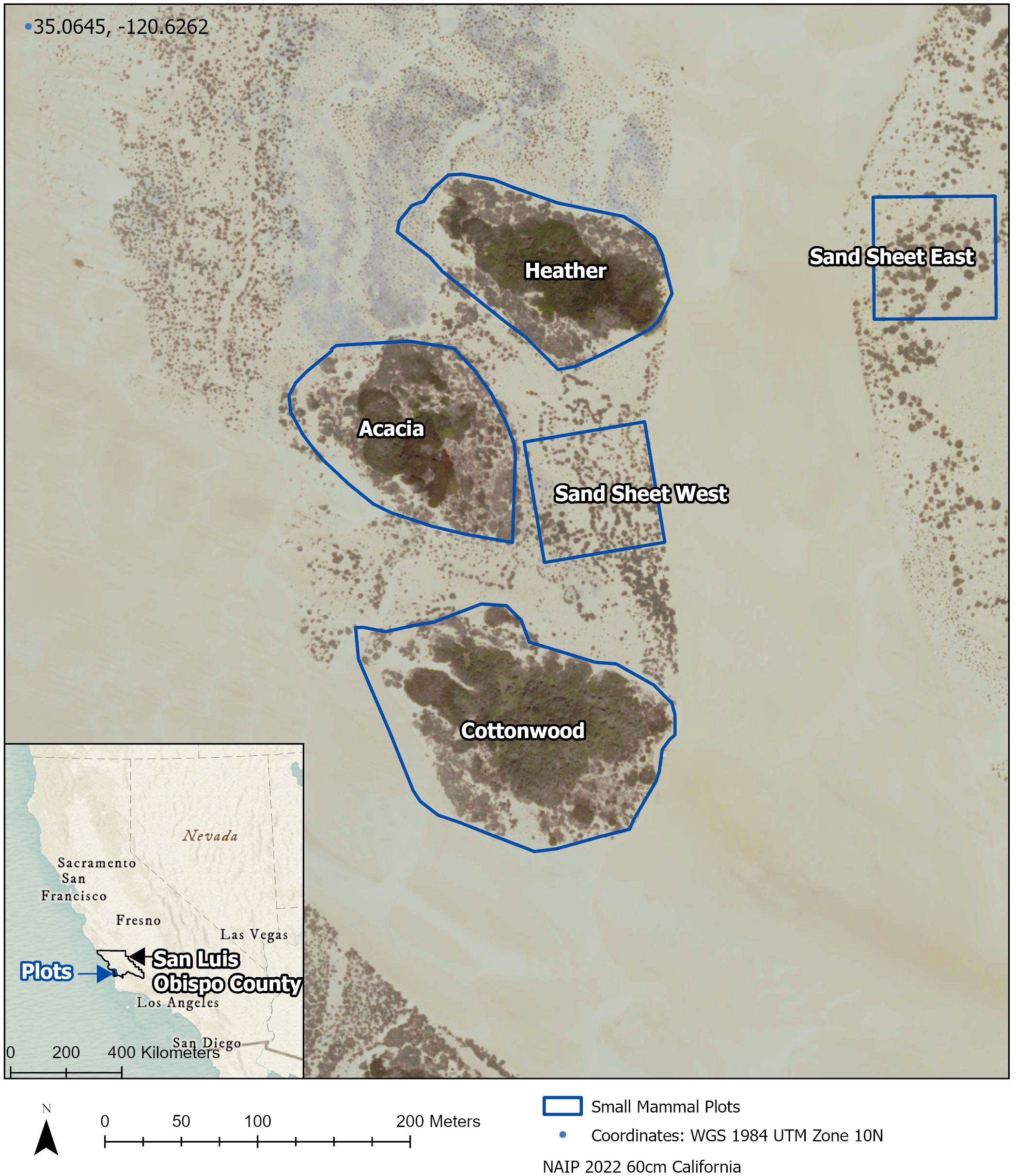
Figure 1 Map of five small mammal survey plots at Oceano Dunes State Vehicular Recreation Area in Oceano, CA.

Each plot was sampled using a standardized grid with 8 stations at 40-meter intervals. There was always at least 10 meters of habitat between the plot and the vegetation edge. To control for the two dominant plant alliances, half of the stations were placed in the willow alliance and half were placed in the scrub alliance at Cottonwood, Heather, and Acacia. The Sand sheet vegetation is scrub throughout, no willow vegetation was planted or has become established, so no vegetation standardization was needed for grid placement.

2.2 Data collection

To determine which monitoring method yields greater detection probability of the six species two different survey techniques were used: baited live traps and baited camera traps.

2.2.1 Live trapping

Live trapping was conducted at the five plots across quarters (spring, summer, fall, winter). Due to constraints of equipment and personnel, all five plots could not be trapped on the same dates. Instead, three islands were trapped first, followed by the two sand sheet plots. Spring live trapping occurred between March 17 and May 1, summer trapping between June 7 and 25, fall trapping between September 14 and 22, and winter trapping occurred between December 6 and 19. Two baited Sherman XL live traps were placed at each station (within 2 meters) for a total of 16 traps across 8 stations per plot. Traps were dedicated to this study. The same traps were used each trapping session and were not cleaned since they were only used in a single location/habitat. Traps were baited each night with either autoclaved rolled oats (recleaned horse oats) or rolled oats for human consumption. Traps were set as close to sunset as possible and checked as close to sunrise as possible. Traps were set in the same manner the following night, for a total of three nights per station per trapping session. Upon checking traps, the species captured were recorded. For each species, detection histories were created for each station for each night where a ‘1’ was given if an individual of the species was trapped and a ‘0’ if an individual of the species was not trapped. The detection history was subsequently the length of the trapping session, three nights, for each of the four seasons.

2.2.2 Camera trapping

Following live trapping, baited camera traps were deployed at the five plots. We employed a four-night lag between live trapping and camera trapping, to allow a ‘rest’ period. It has been shown that some species, such as kangaroo rats, systematically forage and return to areas of high reward on subsequent nights (Price and Correll, 2001), and that some species, or individual California voles, may become “trap happy” or “trap shy” (Hopkins 2022, unpublished thesis). If it occurred, either behavior could impact detection after the first live capture, so the rest period was intended to mitigate the effects of such behavior being transferred from one detection method to the other. Spring camera trapping occurred between March 23 and May 8, summer trapping between June 12 and July 2, fall trapping between September 20 and 29, and winter trapping between December 10 and 29. The same grids were used as for the live trapping protocol. One camera was placed at every station (within 2 meters) of the 8-station live trapping grid, for a total of 8 cameras per plot. Cameras were set for a total of three nights per station per trapping, making it possible to compare camera and live trap detections and occupancy across eight stations and three nights for each plot each season.

Bushnell Trophy Cam HD Essential E3 cameras were set to capture three images per event (i.e., three images per instance of motion detection). There was a one-minute delay between events to avoid excessive images of the same individual. Camera traps were mounted, camera lens facing down, to a metal 0.9 meter U post so that the view was of the animal’s dorsal surface (Figure 2). Each U post had a PVC pipe (3.8 centimeter diameter) attached to it, a few inches below the camera, into which the bait was inserted. The U post was set so that the PVC pipe was ~2.5 centimeters from the ground, allowing the bait to flow down via gravity to replace the bait that was consumed. Traps were baited with either autoclaved rolled oats (recleaned horse oats) or rolled oats for human consumption.

Figure 2

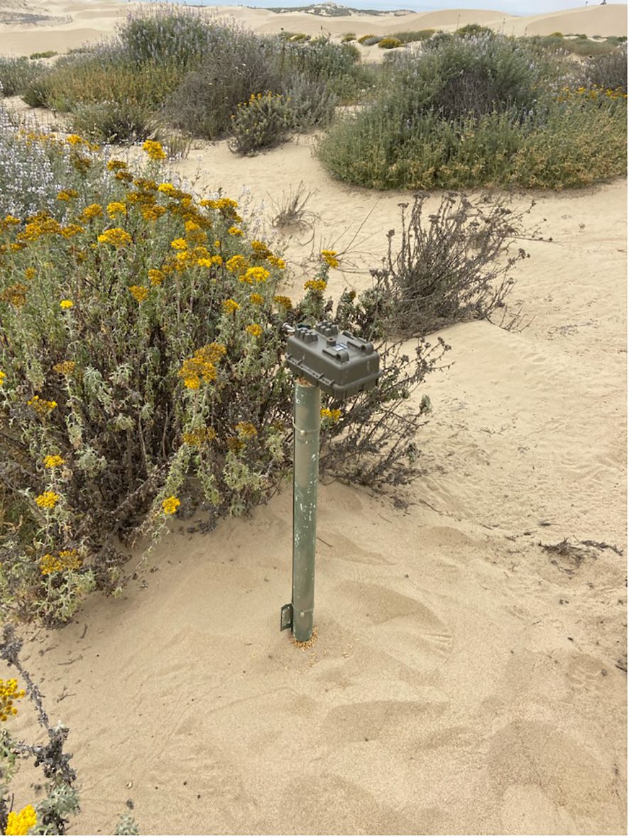
Figure 2 Set up of baited camera station used for surveys at Oceano Dunes State Vehicular Recreation Area in Oceano, CA.

Unlike live trapping where bait was set every night, the bait was only set when the cameras were deployed (night one). This meant the bait ran out during the camera trap session. This was intentionally done to account for varying behavior across rodent species, suspecting some may be less likely to approach high activity stations. This methodology is also low effort, as no additional trips to the station are required until camera collection. Most of the station’s bait lasted one night or two at the most, although this varied.

Once the camera images were collected, we used the R package “camtrapR” to organize the raw images (Neidballa et al., 2016). Folder directories were created for each plot and station using the ‘createStationFolders’ function. Images were renamed using the ‘imageRename’ function so that each image name included the plot, station, date, and time of the image. Once the photos were organized, they were processed through the ML model.

2.3 Machine learning model development

To process the camera trap images and obtain each station’s nightly detection history, a machine learning (ML) model was trained and used. Gabriel Marcelo Santos-Elizondo (G.M.S.E.) utilized YoloV5x, an object detection model, which is part of the YOLO (You Only Look Once) family of models. These are 1-stage detectors that section a picture frame into a grid and then perform object classification on each square in the grid simultaneously (Redmon et al., 2016). YoloV5x was selected for its ease of implementation (a full API is available from Ultralytics, see Supplementary Material), detection speed (runs in real time), and accuracy (outperforming other 1-stage and 2-stage detectors) (Jocher et al., 2020). The model makes use of a convolutional neural network (CNN) as one of its steps. The CNN acts as a feature extractor, pulling information important for object detection from images and storing it for prediction.

The YoloV5x model was pre-trained on the MS COCO 2017 dataset (Lin et al., 2014) consisting of 123k images with an additional 41k images for testing. Pre-training images comprise everyday objects, animals, and plants, and allow the model to learn shapes, colors, and edges, making it easier for the model to identify new target objects, such as our six target species. Pre-training is the first step in developing a robust model for species identification when the available dataset is not large or diverse.

2.3.1 Transfer learning

For our application of species identification, transfer learning was also necessary. Transfer learning follows four steps: labeling, training, validation, and testing. Transfer learning allowed us to train the model specifically on our images of each species, and when combined with hyperparameter tuning, allowed us to create an accurate model specific to our species. Our hyperparameters would not necessarily be the same for other data sets and other species identification objectives. Therefore, we provide a summary of the transfer learning process here but see Supplementary Material for details.

Labeling includes placing a bounding box around a rodent within an image and assigning it to a class where class equals one of the species names. Passing images into the model with class labels, the model’s nodes gather what information is useful for the detection of those classes (in this case species). As the model learns to detect rodents, it learns to ignore non-rodent objects such as other taxa and the background.

Training involves the model learning to detect rodents and ignore non-rodent objects by sending the labeled images through the model. For the initial training, photos of each species were sorted by J.H. and F.V. for labeling and subsequent training. In addition, since we were working with a relatively small dataset compared to that used for pretraining, we implemented image augmentations: flip, noise, and blur, to triplicate our training set for a total of over 3k training images for our final training set.

Validation is accomplished by evaluating various metrics. Training loss, validation loss, and mean average precision (mAP) were checked to confirm that the model had been exposed to a sufficient number of target images and had been trained well (not exhibiting high bias or high variance).

The initial iteration of testing followed labeling, training, and validation, whereby the model was run on an initial set of 400 random images collected across all stations of the spring and summer (2021) camera deployment. Each test run identified the species (class) in the 400 test images. The identifications were reviewed and corrected (if necessary) by J.H. The correct and corrected images were then used for the next iteration of training, which was then followed by iterations of validation and testing.

2.3.1.1 Iterations

This process (training, validation, testing) uses the results of the previous iterations (correct and corrected test images) for training and validation. Following the training and validation, a new random sample of 400 images was used for testing. Thus, completing an entire iteration. The model was re-trained for 150 epochs on the new training set (previous testing set), wherein each epoch the entire set of training data was passed through the model. Iteration continued until the model had a high probability of true positives and a low probability of false positives for each species (see results), which took four iterations. The final test images (fourth run) were fed through the model to complete measurable construction. As a last measure, the whole set, training-validation-testing was passed to the model for training. This allows the model to use all the information available. After this process to optimize the model was iterated four times, the model could identify the six species accurately and consistently (see results).

2.3.2 Model employment

Once model performance metrics demonstrated the model could identify the six species accurately and consistently (see results), a threshold value (0–1) had to be selected for when the model should accept the species identification (i.e.: report a result for an image). For the model to accept and report the species identification, the prediction confidence (a number between 0–1 for each object detected by the model) must be greater than or equal to a threshold. Confidence values are produced for all objects detected by the model. So, even if there is a small chance the object within the bounding box is not species A but species B, the model will produce a confidence value for both. Effectively the model produces low confidence values for unlikely species and high confidence values for likely species within a detection location. The confidence threshold makes the model ignore the unlikely species and only accept and report the likely one. Setting a high threshold (> 0.9) means the model only accepts species identification if the prediction confidence is over 90%. This could lead to individuals being ‘missed’. A low threshold (< 0.5) could lead to incorrect identifications (false positives). We empirically estimated the threshold by running the model on test images under different thresholds (0.5, 0.7, 0.9) and reviewing the model results. Empirically, at 0.5 some individuals were incorrectly identified, or the model accepted two identifications since the model only had to be 50% certain. With the threshold at 0.9, some images with lower quality, for example where the tail was not as visible or the individual was moving, had individuals that were missed. Figure 3 shows the model result for one image that had low confidence (0.83). Setting the threshold at 0.9 would have led to the species being missed. Therefore, through this and other examples, we determined that at 0.7 at least one of the three images (per event) should be accepted as identifiable while minimizing the chance of false identifications. Rather than assuming identifications were always accurate, the species’ presence per station per night were manually confirmed by J.H.

Figure 3

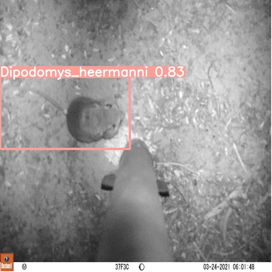
Figure 3 Model result for one image of Dipodomys heermanni with model threshold at 0.7. Accepted identification in this image is shown as a salmon-colored bounding box around the target with a species prediction and a confidence value (0.83). Given the lower confidence in the species prediction for this image (0.83), setting the model threshold at 0.9 would have led to the individual being missed.

The model was then employed on the entire set of camera trap images (> 200,000). A python (Van Rossum and Drake, 1995) script written by G.M.S.E. was utilized to append each image’s filename with the species identification. If an image contained multiple individuals or multiple species, the model could identify all individuals in the image and the script could append all the relevant names to the image name. Using the appended filenames, detection histories (using 0 and 1) for each species were created (using python script) for each station per night for the length of the camera deployment, three nights.

2.4 Data analysis

To test whether cameras vs live traps yield greater detection for the six species, the detection histories for both methods were combined with the method (live or camera) included as a detection covariate. The “unmarked” package (Fiske and Chandler, 2011) in R (R Core Team, 2018) was used to determine detection probabilities for all six species. The function “occu” was used to fit the single season occupancy model of MacKenzie et al. (2002). The MacKenzie et al. (2002) model assumes positive identifications are accurate. To ensure this assumption was not violated, for each species, each station, and each night, one image identified by the YoloV5x model was manually confirmed by J.H., meaning we satisfied the assumptions of the model. Probability of detection was modeled as a function of two additional observer covariates: season (fall, winter, spring, summer), and dominant vegetation (willow or scrub). Previous work (Hopkins 2022, unpublished thesis) has demonstrated an effect of dominant vegetation type on detection probabilities for these species and therefore needed to be included. We also compared the naïve trap success from cameras and live traps to each other via a Wilcoxon Sign-Rank test.

To compare occupancy rates across the two detection methods, the detection histories were analyzed separately, but using the same global model for both data sets. As above, the “unmarked” package and “occu” function were fit to single season occupancy models. Probability of detection was modeled as a function of two observer covariates: season (fall, winter, spring, summer), and dominant vegetation (willow or scrub). Probability of occupancy was modeled as a function of two site covariates: season (fall, winter, spring, summer), and dominant vegetation (willow or scrub).

For all analyses, we built global models to test all possible combinations of model covariates. Package “AICcmodavg” was used to compute the MacKenzie and Bailey (2004) goodness-of-fit test for single season occupancy models based on Pearson’s chi-square through 1000 simulations (Mazerolle, 2020). Models were ranked with c-hat scores from the goodness-of-fit test to ensure best models were also a good fit to the data. Model ranking was done using the “MuMln” package, using AIC for over dispersed data adjusted for small sample size (QAICc) and considering c-hat (Barton, 2022). Models with a ΔQAICc ≤ 2.0 of the top model were considered competitive. We used model-averaging from the “AICcmodavg” package to calculate detection and occupancy probabilities using the best fit models (Mazerolle, 2020).

To provide further insight into the difference in occupancy estimates from the camera data versus live data, we calculated the minimum (naïve) occupancy separately for both data sets. The minimum occupancy is determined by calculating the proportion of sites that had at least one visit across the three-night deployment out of the total number of sites.

3 Results

3.1 ML model for camera image processing

The ML model performed well at identifying the six species based on model metrics. Model health was determined by the training loss and validation loss curves (Figure 4) which should follow similar trends, decreasing to a point where the model has learned all it can from the available data. The model had healthy training and validation loss curves, not displaying signs of low bias high variance (overfit) or high bias low variance (underfit) (Figure 4).

Figure 4

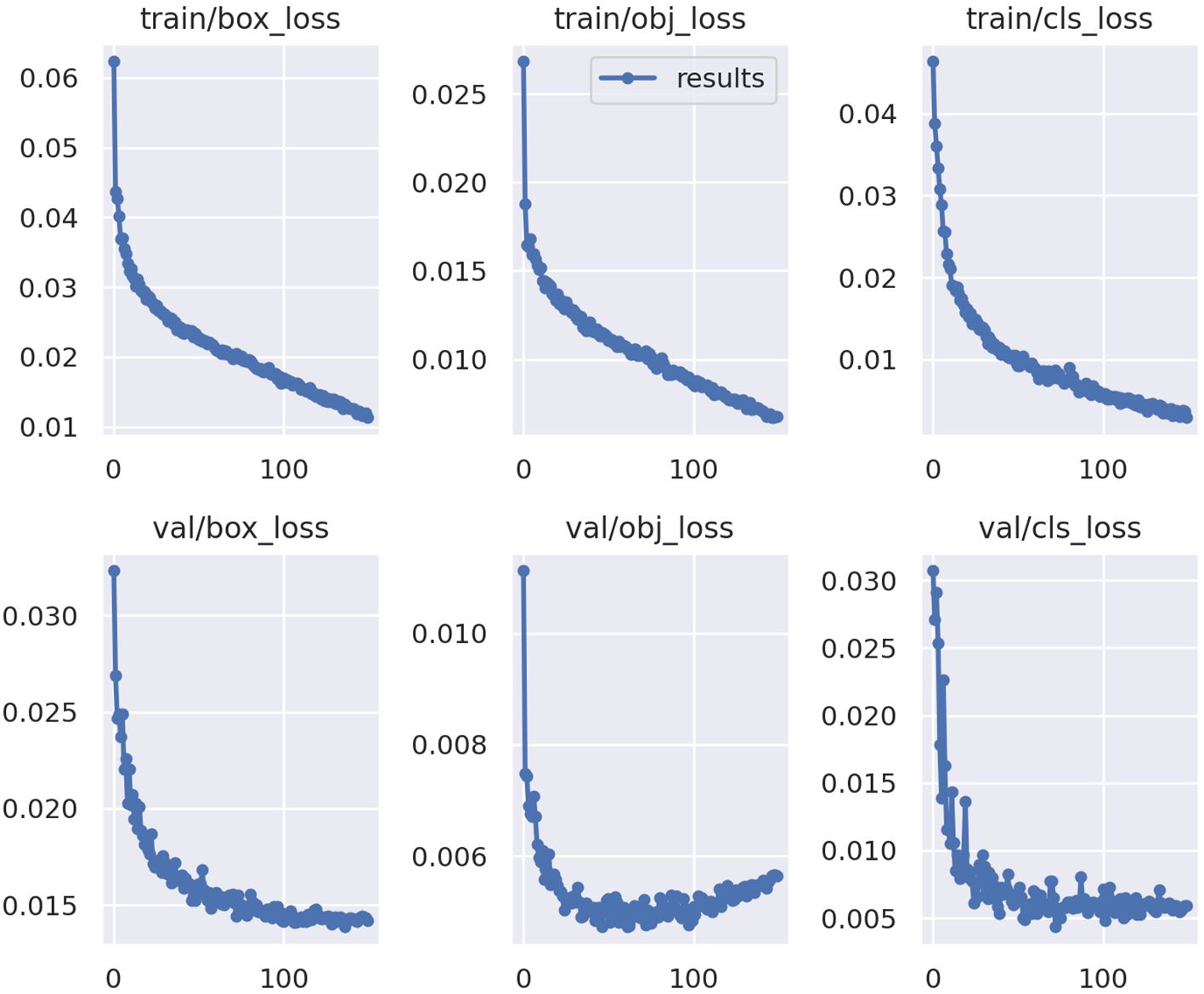
Figure 4 Training loss and validation loss curves for the YoloV5x model. Y-axis is loss calculated from predicted bounding boxes in images (box_loss), probability an object exists within the predicted box (obj_loss), and class versus ground truth (cls_loss) for both training (train) and validation (val). The X-axis is the number of times labeled data was passed through the model for training (0–150). Graphs from Ultralytics (Jocher et al., 2020).

Model performance was also evaluated by reviewing the precision, recall, and mAP curves, where mAP combines the precision and recall of the model (Figure 5). The individual mAP curves for each class (species), and the mAP curve combining all classes, show that precision and recall are both high (Figure 5).

Figure 5

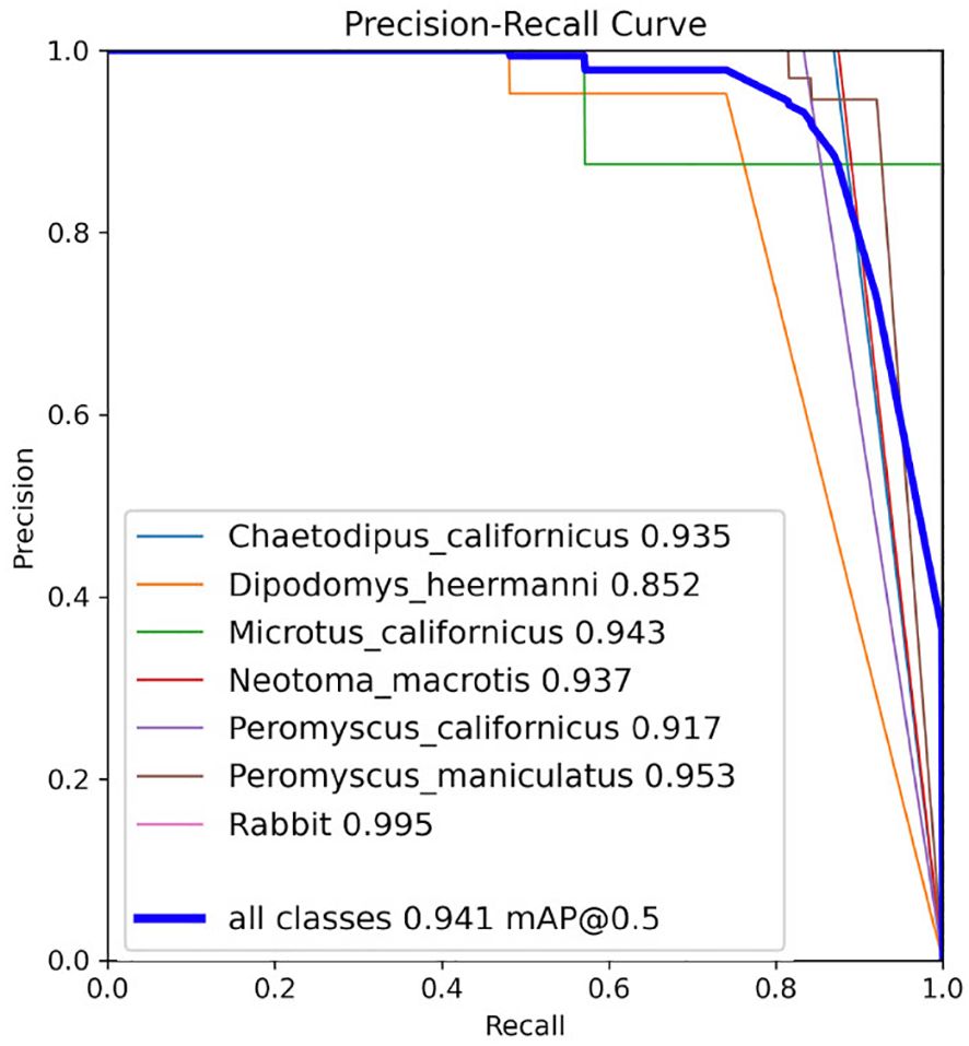
Figure 5 Precision, recall, and mAP metrics for the YoloV5x model on the test set from the last training. The number beside each class (inset box) represents class-specific mean Average Precision (mAP) and the blue line for mAP @ 0.5 represents mAP over all classes with an IoU threshold of 0.5. Graph from Ultralytics (Jocher et al., 2020).

The confusion matrix shows the YoloV5x model did well at predicting each species (Figure 6). The matrix shows the percent of true predictions (known positives) based on testing 10% of the photos available for each species, where these photos had not been supplied for training. Tests were on 15–38 photos per species, except Microtus californicus where only 7 testing photos were available. Reithrodontomys megalotis is included even though it was only detected in Spring 2021 and only by cameras (< 10 images). Therefore, the model was only trained on a small set of images and only had one image to test (which it got right). This species was not included in any analyses or inferences. Figure 6 shows that the largest possible source of confusion was false positives from the background. This, and the limited cross-species confusion, was mitigated by manual human confirmation of at least one positive image per species, per station, and per date when building the detection histories (see methods).

Figure 6

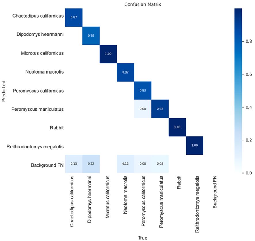
Figure 6 Confusion matrix showing the percent of true predictions for 10% of images per species which were held back for testing. Darkest color represents the lowest confusion. Results are for the empirically determined confidence threshold of 0.7 which was used by the model in AI identification of species from camera images. See text for information regarding Reithrodontomys megalotus. Background FP represents the amount of ‘False Positive’ detections on images without the target species (see text for false positive mitigation measure). Image from Ultralytics (Jocher et al., 2020).

3.2 Detection comparison

Only two species were detected enough on the Sand sheet plots to support an occupancy analysis across all five plots: D. heermanni and P. maniculatus. For the other four species, the analysis was done using only data from Cottonwood, Heather, and Acacia plots. As expected, for all species, naïve trap success (i.e.: detection) was higher when detected through camera traps compared to live traps (Table 1). For an N=6 (species in Table 1) comparison of the trap success across two detection methods, the Wilcoxon Sign-Rank W = 0 with p <0.05 (cannot calculate the exact p-value for N<10).

Table 1

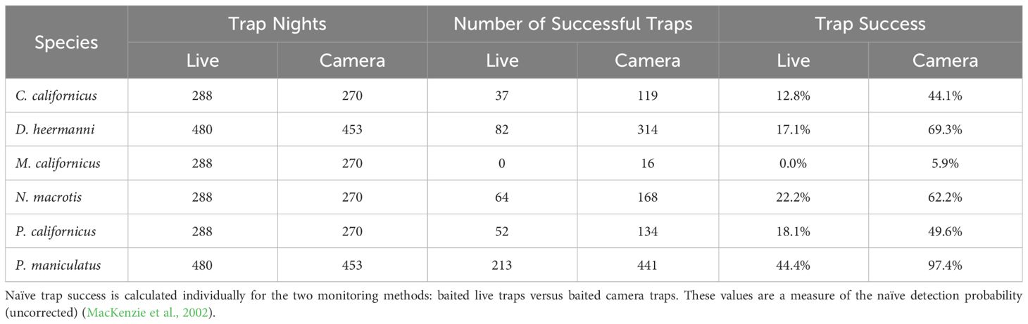
Table 1 Summary of naïve trap success (captures divided by trap nights) for all four seasons (spring, summer, fall, winter) for Chaetodipus californicus, Dipodomys heermanni, Microtus californicus, Neotoma macrotis, Peromyscus californicus, and Peromyscus maniculatus.

3.2.1 Model selection for detection comparison

For all species, detection method (camera or live) was included in the top-ranked model (ΔQAICc ≤ 2.0). Dominant vegetation was included in the top-ranking models for four species C. californicus, D. heermanni, N. macrotis, and P. maniculatus. Season was included in the top-ranking models for three species: C. californicus, N. macrotis, and P. maniculatus. These results test a prediction and are summarized in Table 2.

Table 2

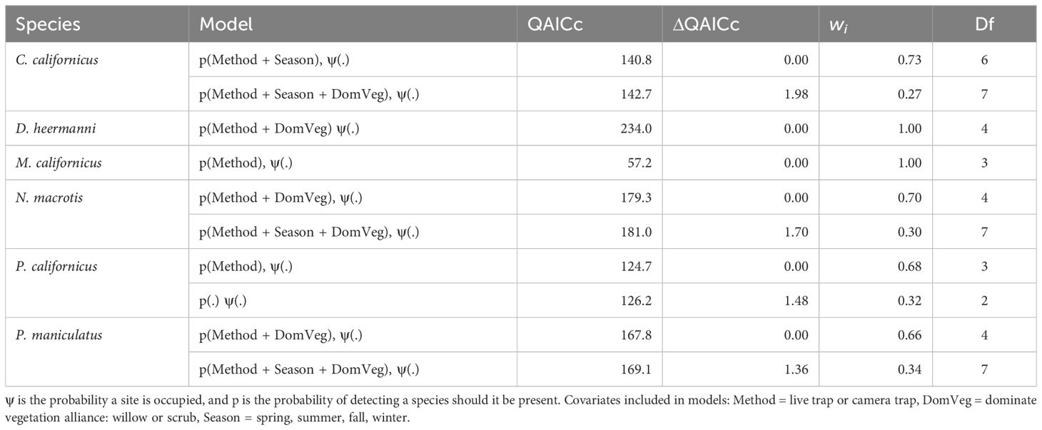
Table 2 Competing (ΔQAICc ≤ 2.0) single season landscape occupancy models with live and camera trap data pooled, for Chaetodipus californicus, Dipodomys heermanni, Microtus californicus, Neotoma macrotis, Peromyscus californicus, and Peromyscus maniculatus.

3.2.2 Detection probability

As predicted, camera traps yielded greater detection probability for all species compared to live traps. This was true for both naïve trap success (Table 1) and corrected detection probability (MacKenzie et al., 2002). These results test a prediction and are summarized in Figure 7. Details for each species are presented below.

Figure 7

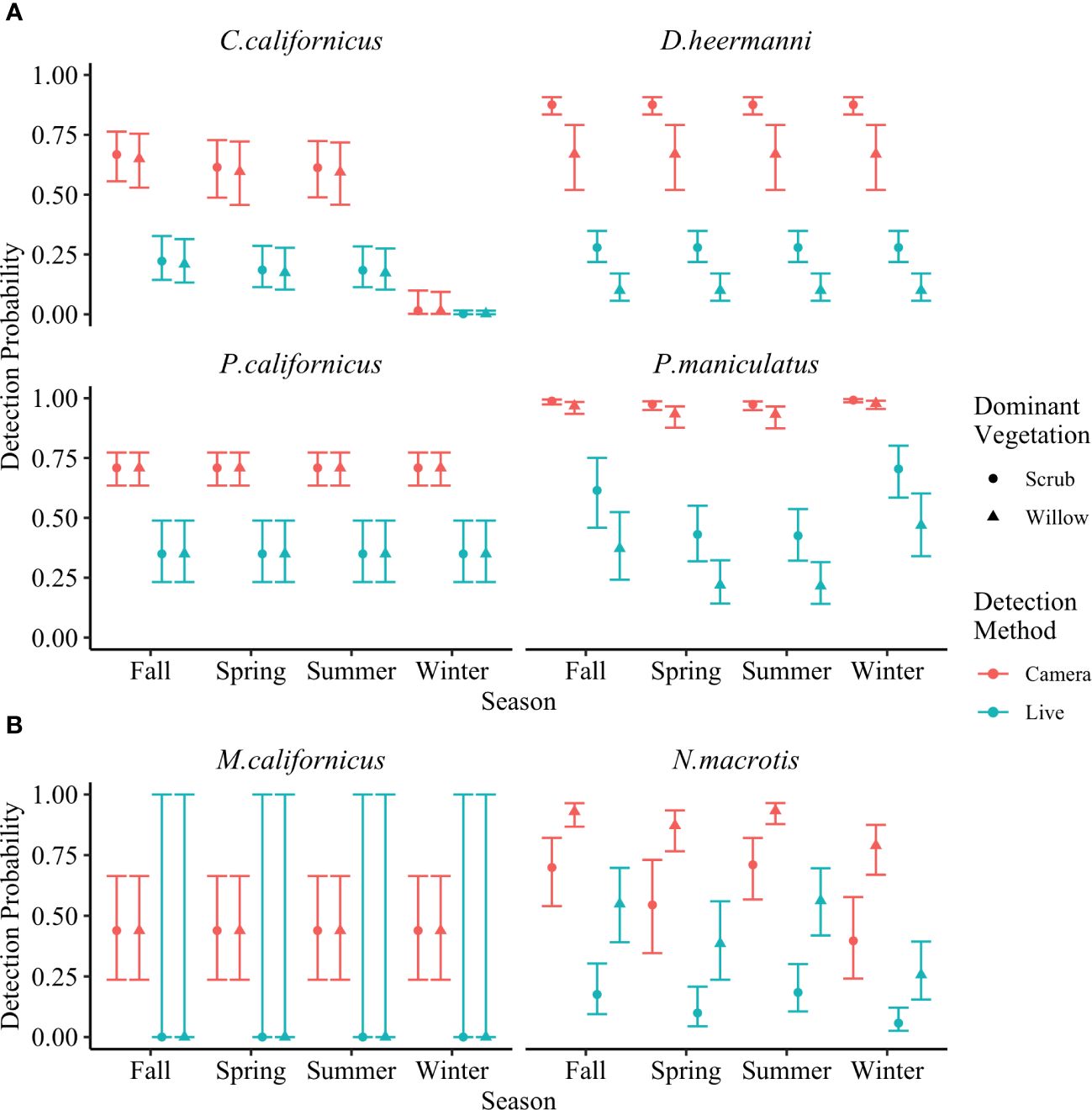
Figure 7 Detection probability for (A) Chaetodipus californicus, Dipodomys heermanni, Peromyscus californicus, Peromyscus maniculatus, and (B) Microtus californicus and Neotoma macrotis across four seasons of deployment analyzed using single season occupancy models (MacKenzie et al., 2002). Detection methods are through baited camera stations or baited live traps. Dominant vegetations are willow dominated or scrub dominated. Error bars represent 95% confidence interval. Detection probability for all species was greater through baited camera stations than through baited live traps.

C. californicus, D. heermanni, P. californicus, and P. maniculatus had significantly higher detection probability through camera traps versus live traps across both willow and scrub dominated stations (Figure 7A).

Considering dominant vegetation as a covariate, detection probability for D. heermanni through cameras was 0.88 in scrub (CI = [0.83, 0.91]) and 0.67 in willow (CI = [0.52, 0.79]), while through live traps it was 0.28 in scrub (CI = [0.22, 0.35]) and 0.10 in willow (CI = [0.05, 0.17]). P. californicus detection probability did not include dominant vegetation as a covariate and through cameras was 0.71 (CI = [0.64, 0.77]) while through live traps it was 0.35 (CI = [0.23 0.49]).

C. californicus and P. maniculatus both showed some influence of dominant vegetation and season on detection probability, with season being weak except for C. californicus in winter. C. californicus had significantly lower detection probability for both methods in winter compared to the other three seasons. Across the other three seasons and both dominant vegetations, C. californicus detection through cameras ranged from 0.59 to 0.67 (CI = [0.46, 0.76]) while through live traps ranged from 0.17 to 0.22 (CI = [0.10, 0.33]). Across all seasons and both dominant vegetations, P. maniculatus detection through cameras ranged from 0.93 to 0.99 (CI = [0.87, 0.99]) while through live traps ranged from 0.22 to 0.70 (CI = [0.14, 0.80]).

Within each dominant vegetation category, N. macrotis had significantly higher detection probability through camera traps versus live traps (Figure 7B). Across all seasons, detection probability in willow stations ranged from 0.79 to 0.93 (CI = [0.67, 0.96]) for cameras and 0.26 to 0.56 (CI = [0.15, 0.70]) for live traps, which was higher than scrub stations which ranged from 0.40 to 0.71 (CI = [0.24, 0.82]) for cameras and 0.06 to 0.18 (CI = [0.03, 0.30]) for live traps.

M. californicus had zero captures across all live trapping surveys, subsequently detection probability is zero and the confidence interval is incalculable. While there were zero detections through live traps, there were multiple camera detections. The detection probability through camera traps was 0.44 (CI = [0.24, 0.66]). Qualitatively it is clear there was greater detection through camera traps.

3.3 Occupancy comparison

3.3.1 Model selection for occupancy comparison

Top ranking models (ΔQAICc ≤ 2.0) for each species analyzed using camera data versus live capture data are shown and summarized in Table 3. M. californicus had zero live captures and C. californicus had insufficient live captures and therefore both were excluded from this analysis. Dominant vegetation was shown to have an influence on occupancy probability for D. heermanni and N. macrotis in both analyses of camera data and live capture data. Analysis of camera data showed an influence of dominant vegetation on P. californicus occupancy probability, but the live capture data analysis did not, while the opposite was true for P. maniculatus. Neither analysis of the camera nor live data showed an influence of season on occupancy for these species.

Table 3

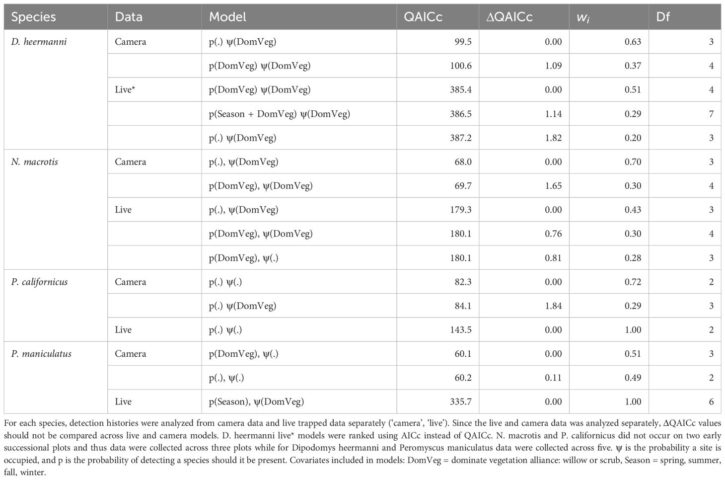
Table 3 Competing (ΔQAICc ≤ 2.0) single season landscape occupancy models for Dipodomys heermanni, Neotoma macrotis, Peromyscus californicus, and Peromyscus maniculatus.

3.3.2 Comparing occupancy probability between camera and live trapping methods

Our prediction that occupancy probability would be greater when analyzed using camera data versus live trapped data was supported. Specifically, within each dominant vegetation type, all species had higher occupancy probabilities when analyzed from camera traps, and since occupancy is estimated from detection, all species also had higher detection probabilities with camera traps. These results test a prediction and are summarized in Figure 8.

Figure 8

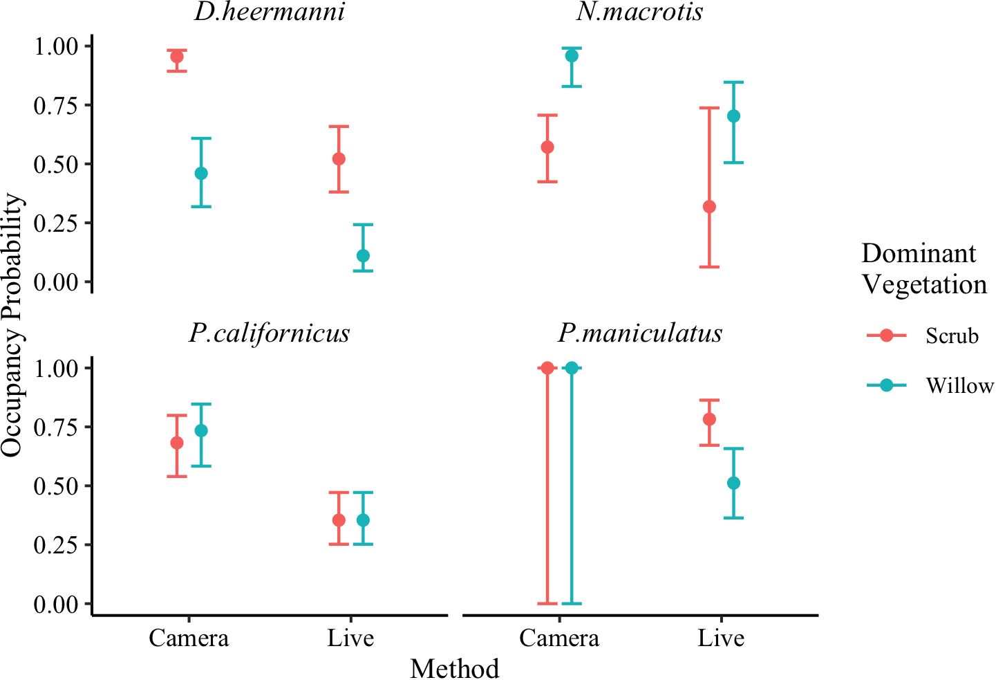
Figure 8 Model averaged (Table 3) occupancy probability for Dipodomys heermanni, Neotoma macrotis, Peromyscus californicus, and Peromyscus maniculatus from camera trapped data versus live trapped data analyzed separately using single season occupancy models (MacKenzie et al., 2002). Dominant vegetations are willow dominated or scrub dominated. Error bars represent 95% confidence intervals. Neotoma macrotias and Peromyscus californicus did not occur on two early successional plots and thus data were collected across three plots while for Dipodomys heermanni and Peromyscus maniculatus data were collected across five plots. There were not sufficient live captures of M. californicus or C. californicus, so they were excluded from analysis.

Our prediction that patterns in occupancy probability would be the same across the two monitoring methods was only partially supported. An influence of season on occupancy was not found through either analysis for any species included. The influence of dominant vegetation on occupancy across the two analyses varied. These results test a prediction and are summarized in Figure 8, while individual species are discussed below.

Occupancy probability was higher within each dominant vegetation type for D. heermanni when analyzed using camera data versus live trap data (Camera: ψ_Scrub = 0.95, CI [0.89, 0.98], ψ_Willow = 0.46, CI [0.32, 0.61], Live: ψ_Scrub = 0.52, CI [0.38, 0.66], ψ_Willow = 0.11, CI [0.04, 0.24]) (Figure 8). Both analyses using live and camera data, demonstrated a strong influence of dominant vegetation on this species occurrence. Occupancy probability was higher for N. macrotis within each dominant vegetation type when analyzed using camera data versus live trap data (Camera: ψ_Willow = 0.96, CI [0.83, 0.99], ψ_Scrub = 0.57, CI [0.42, 0.71], Live: ψ_Willow = 0.70, CI [0.51, 0.85], ψ_Scrub = 0.32, CI [0.06, 0.74]) (Figure 8). However, given the large confidence intervals associated with the live trapped estimates, N. macrotis was the only species where occupancy probability was not significantly higher in cameras, though occupancy probability was qualitatively higher. The analysis using camera data demonstrated a strong influence of dominant vegetation on this species occupancy probability while the analysis using live data showed a weak influence of dominant vegetation. Thus the prediction that the two detection methods would ascribe the same importance to habitat attributes was not supported for this species (Figure 8).

Across both dominant vegetation types, occupancy probability for P. californicus was higher when analyzed using camera data versus live trap data (Camera: ψ_Willow = 0.73, CI [0.58, 0.85], ψ_Scrub = 0.68, CI [0.54, 0.80], Live: ψ = 0.35, CI [0.25, 0.47]) (Figure 8). Only the analysis using camera data showed an influence of dominant vegetation on this species occupancy, but the influence was weak (CI overlap). Occupancy probability for P. maniculatus was higher when analyzed using camera data versus live trap data (Camera: ψ = 1.00, CI [0.00, 1.00], Live: ψ_Scrub = 0.78, CI [0.67, 0.86], ψ_Willow = 0.51, CI [0.36, 0.66]) (Figure 8). The analysis using camera trap data yielded an occupancy of 1 (441 out of 453 camera trap nights (97%) had a P. maniculatus detection) regardless of dominant vegetation type. When an estimate approaches 1 (or 0), the SE on the logit-scale becomes extremely large (Mackenzie et al., 2017). Once the CI are back transformed, they span 0–1. Therefore, only the analysis using live data showed an influence of dominant vegetation on this species occupancy. Thus the prediction that the two detection methods would ascribe the same importance to habitat attributes was not entirely supported for these two species (Figure 8).

3.3.3 Minimum and corrected occupancy for cameras and live

The minimum occupancy from cameras and live trap data, as well as the corrected occupancy estimate (MacKenzie et al., 2002), are shown in Table 4. In all cases, the minimum camera occupancy is greater than the corrected live trapped occupancy estimate. The average percent difference between the corrected for and minimum occupancy from cameras was 1%, while the difference from live was 18%.

Table 4

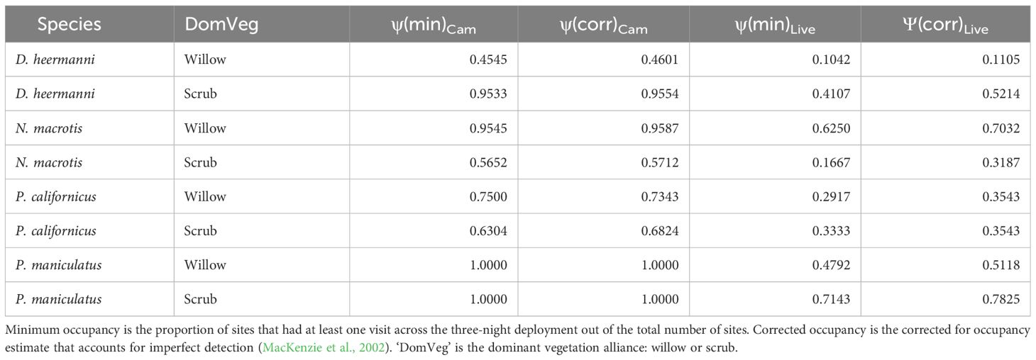
Table 4 Minimum (‘min’) occupancy and corrected (‘corr’) occupancy for Dipodomys heermanni, Neotoma macrotis, Peromyscus californicus, and Peromyscus maniculatus through analysis of data collected by baited camera traps (‘Cam’) versus baited live traps (‘Live’).

4 Discussion

Our prediction that detection probability would be greater from camera traps versus live traps was supported. Subsequently, as predicted, occupancy estimates were greater when analyzed through camera data versus live data. The result of patterns in occupancy analyzed across the two methods varied and depended on the detection method. However, these variable results seem to be influenced by the high amount of camera detections, and therefore better resolution of patterns, relative to live traps.

4.1 Detection

M. californicus was the only species where we could not quantitatively demonstrate the detection probability across the two methods was significantly different. This was due to zero live captures during the four seasons of study such that confidence intervals spanned 0 to 1, and the comparison with camera traps was incalculable. Though live traps might suggest M. californicus did not occupy the study site, there were multiple detections through cameras, qualitatively demonstrating that detection probability is much greater for M. californicus through cameras versus live traps. Indeed, M. californicus is regarded as having cyclic population growth and decline (Lidicker, 2015). But these population cycles likely do not lead to local extinction (absent some years) as suggested by live trapping data. Instead, as suggested by the camera trapping data, the local breeding deme likely persists, though at very low abundance. Management might thus need to focus on this growth and decline population dynamic rather than an extinction-recolonization dynamic.

4.1.1 Cameras yield greater detection

Multiple factors could be influencing why cameras yield greater detection. Trap saturation is a possible drawback of live trapping. Once a live trap is occupied, individuals may approach the station but would not be detected because generally only one individual is captured per trap. Cameras allow for unlimited detections without trap saturation. Cameras are noninvasive and allow detection of rodents without entrapment whereas live traps require entering an enclosure. Live traps can contain urine and feces of con and heterospecifics previously trapped. Both types of odors have been shown to influence rodent behavior (Boonstra and Krebs, 1976; Mazdzer et al., 1976; Daly et al., 1978; Daly et al., 1980). Peromyscus, Chaetodipus, and Dipodomys avoid traps containing these odors during the non-breeding season (Daly et al., 1978; Daly et al., 1980), deterring them from entering traps and being detected. This deterrence could be mitigated by washing each trap after each capture. But this only shows the increase in effort needed to maximize the detection probability of live traps. Herein we consider live trapping results over three-night sessions. More nights are expected to increase detections of rarer species but would come with more effort. One suggestion is to trap for 11 consecutive nights (Hice and Velazco, 2013). Imagine the Herculean effort of trapping for 11 consecutive nights and washing each trap after each capture. Despite the effort, species vary in their likelihood of entering live traps (Gurnell, 1982; Stokes, 2012). Studies of other rodents show that approximately half the individuals in a population are trap-able and that previous experience with traps influences their behavior (Gurnell, 1982). In these studies, marked animals have higher trap-ability than unmarked animals, and probability of recapture can be greater than probability of initial capture (Tanaka, 1963; Gurnell, 1972, 1982). Therefore, some individuals in a population may never be captured due to their individual behavior. One final difference is the induced stress response caused by entrapment (Kenagy and Place, 2000; Fletcher and Boonstra, 2006; Bosson et al., 2012). The resulting psychological response to entrapment influences trap mortality (Gurnell, 1982), and the stress could even affect individuals following release. Trap mortality is also influenced by moisture and temperature (Gurnell, 1982). Moisture could be from weather or self-urination. Once rodents’ fur is damp, individuals are unable to thermoregulate as effectively (Perrin, 1975), and increased trap deaths have been reported following rain (Gurnell, 1982). For all these reasons, if understanding occupancy provides sufficient knowledge, cameras appear to be superior to live trapping for detecting rodents and should be specifically considered when studying rare, endangered, threatened, or cryptic species.

4.2 Occupancy

The minimum (uncorrected) camera occupancy (Table 4) was greater for all species than the corrected live capture occupancy estimate. For example, through cameras, P. maniculatus was detected at every single station at least one night, and therefore occupied every station. However, for live trapping, the corrected occupancy probability was 51% at willow stations and 78% at scrub stations. This demonstrates a potential issue when using live traps to understand rodent species occurrence because occupancy is predicted to be underestimated. In contrast, the minimum camera occupancy is very similar to the estimated camera occupancy, demonstrating that detection through cameras requires little correction, if any, for imperfect detection. For the four species included in the occupancy analysis, the per night detection probability (Figure 7) is so high that the detection probability (averaged across four seasons and both vegetation types) for a three-night session is greater than 0.97. This indicates correcting for detection is not necessary even over just three nights and without rebaited camera stations. While we do not advocate for using uncorrected estimates of occupancy, for budget limited efforts where statistical analyses are not practical, land managers may consider this as a reasonable approximation of occupancy.

The underestimation of occupancy from live traps could be influenced by the interaction of live traps and detection, with live traps possibly conferring increased heterogeneity in detection for reasons discussed previously (strap saturation, odors, behavior, etc.). If live traps confer heterogeneity in detection, and those sources are not able to be modeled (i.e., trap shy individuals, temporal partitioning among species approaching traps) the occupancy estimates from live trap data will be downwardly biased. Additionally, live traps can be saturated, allowing only two individuals to be captured per station such that additional species (>2) would be missed. Inferring cameras are more neutral to rodents, sources of detection heterogeneity caused by live traps may be removed. Likewise, cameras allow unlimited detection and remove possible bias from trap saturation. Subsequently, there is less possibility of bias in occupancy estimates from cameras. Nevertheless, we acknowledge that both live and cameras could still be influenced by unmodellable sources of detection heterogeneity, such as abundance (MacKenzie et al., 2017). However, the greater mean detection probability from cameras could reduce this possible biased effect on occupancy estimates.

4.2.1 Patterns in occupancy

The result of patterns in occupancy estimates analyzed across the two methods varied for some species and depended on the detection method. This could lead to a larger type II error (a false negative when a difference does actually exist) under live trapping. For example, the camera data analysis found N. macrotis occupancy to be strongly influenced by dominant vegetation, while the live data analysis found this influence to be weak and may have led to a type II error if only the live data was considered. This seems intuitive if we accept that live trapping data have a reduced ability to detect, and therefore resolve differences in, occupancy across site covariates. Likewise, live traps could lead to a pattern being demonstrated through analyses but one that is a result of live trapping, not species occupancy (e.g., trap saturation is more likely at willow stations). For more accurate estimates of occupancy through live trapping, a longer survey method may be required. It has been demonstrated that longer trapping sessions (survey nights) are necessary when surveying small mammals through live traps to detect all species (Hice and Velazco, 2013). Our analysis of occurrence through live trapping may have yielded greater inference power if the survey length was greater, given the low per night detection probability achieved through live traps (Figure 7). However, increasing the survey length would substantially increase the effort and not support our development of a practical and sustainable monitoring methodology. We also acknowledge the possibility that cameras could have issues with detecting small influences of site attributes on species occurrence, which may have been true for P. maniculatus. The camera data analysis found no influence of dominant vegetation, while the live data analysis found a strong influence of dominant vegetation, with occupancy probability being higher in scrub. It is possible that with such good detection through cameras, and subsequent high occupancy estimates (1.0 for P. maniculatus), small influences of site covariates could be undetectable. These possibilities, and the possible effects on occupancy analyses, might merit further investigation.

4.3 Live traps versus camera traps: effort and prospects

4.3.1 Live traps versus camera traps: effort

While the specific community assemblage of rodents in question may affect the ability to monitor rodents through camera traps, rodents can be identified at the species level through camera images (De Bondi et al., 2010; Gray et al., 2017; Thomas et al., 2019). We found that, while cameras collect a huge number of images, ML models can be used to drastically reduce effort.

To better illustrate this finding, we estimated the effort (hours) spent across live trapping, camera trapping, and camera trapping with ML for this project (Figure 9). Since all the tasks (live trapping, camera trapping, and ML model development) were carried out for this study, the time to complete them was known and used. Live trapping effort was calculated by estimating the time spent: in the field setting and processing traps (processing includes time for traditional mark-release-recapture), travel to and from plots, and entering data into a database. For cameras, the effort was calculated by estimating the time spent: to deploy and collect cameras, travel to and from plots, and upload and manually sort all images into species folders. For cameras with ML, effort was calculated by estimating the time to: deploy and collect cameras, travel to and from plots, construct the ML model, identify images for initial training, label the images for training, review/correct test images, and upload camera images for model processing. The time for ML model construction entails choosing hyperparameter values and establishing a workflow. The task that was not performed entirely was the manual sorting of images into species respective folders. To estimate that required time, a subset of images was manually identified and sorted and the time spent was extrapolated to the number of images collected in total. The effort estimates presented include only ‘active’ time (not CPU time) and assume experienced and knowledgeable researchers conducting all the work (no personnel training).

Figure 9

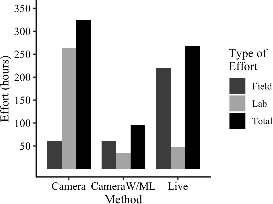
Figure 9 Estimated effort (hours) spent for this project across the two methods of data collection. Cameras were compared for manual photo processing versus photo processing with the ML model. ‘Cameras with ML’ lab effort includes time estimate to: train model, review/correct images in testing, choose hyperparameters, and establish a workflow. All estimates are based on active time of experienced and knowledgeable researchers conducting the work.

The effort estimated across the methods demonstrates the drastically reduced effort of cameras when paired with ML models for image processing (Figure 9). Trapping with live traps would take 267 estimated hours, trapping with cameras using manual image processing would take 324 estimated hours, but trapping with cameras utilizing a ML model would take only 95 estimated hours. In addition, once the model is fully trained, the lab effort declines substantially, only requiring the time to upload the images and begin model processing (runs in the background).

The effort applied to live trapping small mammals in Mediterranean habitats is variable. For example, recent studies have deployed live traps for between three and seven consecutive nights (Diffendorfer et al., 2012; Borchert and Borchert, 2013; Moreno and Rouco, 2013; Polyakov et al., 2021; Germano et al., 2023; Ghimirey et al., 2023). Two of these studies have investigated rodent communities with many of the same species as we considered (Germano et al., 2023; Ghimirey et al., 2023). They have both used three consecutive trap nights, as did we. We fully recognize that additional live trapping effort (eg.: adding more consecutive nights) likely adds species detections (Hice and Velazco, 2013). But we find that would make our overall conclusion, that camera trapping produces more detections with less effort than live trapping, even stronger. For example, there was only one rodent species (Reithrodontomys megalotus) expected to be detected which was not detected over three consecutive nights of live trapping in any of the four seasons. But even that species was detected, though only in Spring 2021, by camera traps (< 10 images).

4.3.2 Live traps versus camera traps: prospects

Future improvement of the ML model through additional training with more images could produce extreme accuracy. Likewise, one could consider rebaiting the camera stations each night for the first session, gathering more photos for initial model training, and possibly making model construction easier. Yet we found that baiting only the first night of deployment still led to very high detection probabilities and kept the field effort low.

Due to YoloV5x’s accuracy and pre-training on the MS COCO 2017 dataset, the model was able to learn to ignore the background. We explored the need to train the model on ‘blank’ images (containing no rodents) with a variety of backgrounds (sand, leaf litter, sticks) but this was unnecessary as the pretraining taught the model to ignore the background.

Though conservation and management focused long-term monitoring is an obvious application, ML could also be implemented for invasive species monitoring. Invasive species are a global problem to ecosystem health (Rinella et al., 2009) and a huge effort is given to the management of invasives (Lodge et al., 2006). If an invasive species has the potential to invade or is potentially present, detecting populations while they are small and localized, focusing on early detection and rapid response (EDRR), is essential (Lodge et al., 2006). However, detecting species while populations are small is difficult, as detection is influenced by abundance (Royle and Nichols, 2003; McCarthy et al., 2013). Invasive rodent species biosecurity, like for Rattus rattus, could be done by deploying web enabled cameras, with ML analytics, that could update managers almost instantaneously of invasive species detection. Likewise, an approach that combines live trapping and camera trapping for invasive species management could make sense. Live traps (or kill traps) could entrap invasives, while camera traps would inform the degree of success of the entrapment/kill effort. This might be particularly meaningful following an attempted eradication, or while running surveillance, for an invasive rodent.

4.4 Conclusions

The current loss of biodiversity and rate of extinctions highlights the need for conservation efforts across all taxa, including small, non-charismatic ones. With 332 rodent species listed on the IUCN red list, there is a need for efficient and effective methods for monitoring their populations. Our study demonstrates that cameras provide far greater detection of rodents compared to live traps and should be considered for detecting rare, listed, or cryptic small rodent species. The greater detection through cameras allows more accurate estimates of occupancy, all of which differed from live trapping estimates, and better insight into the influence of habitat attributes on species occurrence. This noninvasive technique is safer, not requiring entrapment or handling, and could be a valuable contribution to the study of endangered or vulnerable species. Additionally, cameras require low field effort and can be used in conjunction with ML models to provide efficient, accurate, and precise detection of monitored rodent species. For wildlife management and conservation, camera data processed through ML models can be used with occupancy modeling to provide insight into the influence of habitat characteristics, modifications, and changes to species occurrence.

Data availability statement

The raw data supporting the conclusions of this article will be made available by the authors, without undue reservation.

Ethics statement

The animal study was approved by Institutional Animal Care and Use Committee of California Polytechnic State University, San Luis Obispo (Protocol number 1713, 17 January 2018). CDFW Scientific Collection Permit #: S-190250002-19028-001. California State Parks Permit to Conduct Scientific Research and Collections (DPR 65). The study was conducted in accordance with the local legislation and institutional requirements.

Author contributions

JH: Data curation, Formal analysis, Investigation, Methodology, Software, Validation, Writing – original draft, Writing – review & editing, Visualization. GS-E: Data curation, Methodology, Software, Validation, Writing – original draft, Writing – review & editing, Investigation, Visualization. FV: Conceptualization, Funding acquisition, Investigation, Methodology, Project administration, Resources, Supervision, Validation, Writing – original draft, Writing – review & editing.

Funding

The author(s) declare financial support was received for the research, authorship, and/or publication of this article. This research was funded by California Department of Parks and Recreation (award number C1853013) and support from the College of Science and Mathematics’ (Cal Poly) Grant Related Assigned Time program.

Acknowledgments

We thank California Department of Fish and Wildlife, and the California Polyethnic Institutional Animal Care and Use Committee for permitting this research (permit no. S-190250002–19028-001). We thank California Department of Parks and Recreation staff at Oceano Dunes, California, for their funding and assistance in data collection and field work. Special thanks to Stephanie Little and Courtney Tuskan for organizing and assisting field work at ODSVRA. We thank Dr. Clint Francis, Dr. Tim Bean, and Ashley Fisher for assistance on previous drafts of this manuscript. The model used, YoloV5x, was made available by Ultralytics, which we thank for making their software open source and accessible to all.

Conflict of interest

The authors declare that the research was conducted in the absence of any commercial or financial relationships that could be construed as a potential conflict of interest.

Publisher’s note

All claims expressed in this article are solely those of the authors and do not necessarily represent those of their affiliated organizations, or those of the publisher, the editors and the reviewers. Any product that may be evaluated in this article, or claim that may be made by its manufacturer, is not guaranteed or endorsed by the publisher.

Supplementary material

The Supplementary Material for this article can be found online at: https://www.frontiersin.org/articles/10.3389/fevo.2024.1359201/full#supplementary-material

References

Avenant N. (2011). The potential utility of rodents and other small mammals as indicators of ecosystem ‘integrity’of South African grasslands. Wildlife Res. 38, 626–639. doi: 10.1071/WR10223

CrossRef Full Text | Google Scholar

Bailey L. L., Simons T. R., Pollock K. H. (2004). Estimating site occupancy and species detection probability parameters for terrestrial salamanders. Ecol. Appl. 14, 692–702. doi: 10.1890/03-5012

CrossRef Full Text | Google Scholar

Baker P. J., Ansell R. J., Dodds P. A., Webber C. E., Harris S. (2003). Factors affecting the distribution of small mammals in an urban area. Mammal Rev. 33, 95–100. doi: 10.1046/j.1365-2907.2003.00003.x

CrossRef Full Text | Google Scholar

Barnosky A. D., Matzke N., Tomiya S., Wogan G. O., Swartz B., Quental T. B., et al. (2011). Has the Earth’s sixth mass extinction already arrived? Nature 471, 51–57. doi: 10.1038/nature09678

PubMed Abstract | CrossRef Full Text | Google Scholar

Barton K. (2022) MuMIn: multi-model inference. R package version 1.46.0. Available online at: https://CRAN.R-project.org/package=MuMIn.

Google Scholar

Boonstra R., Krebs C. J. (1976). The effect of odour on trap response in Microtus townsendii. J. Zoology 180, 467–476. doi: 10.1111/j.1469-7998.1976.tb04692.x

CrossRef Full Text | Google Scholar

Borchert M., Borchert S. M. (2013). Small mammal use of the burn perimeter following a chaparral wildfire in southern California. Bulletin South. California Acad. Sci. 112, pp.63–pp.73. doi: 10.3160/0038-3872-112.2.63

CrossRef Full Text | Google Scholar

Bosson C. O., Islam Z., Boonstra R. (2012). The impact of live trapping and trap model on the stress profiles of N orth A merican red squirrels. J. Zoology 288, 159–169. doi: 10.1111/j.1469-7998.2012.00941.x

CrossRef Full Text | Google Scholar

Burgin C. J., Colella J. P., Kahn P. L., Upham N. S. (2018). How many species of mammals are there? J. Mammalogy 99, 1–14. doi: 10.1093/jmammal/gyx147

CrossRef Full Text | Google Scholar

Carbone C., Christie S., Conforti K., Coulson T., Franklin N., Ginsberg J. R., et al. (2001). The use of photographic rates to estimate densities of tigers and other cryptic mammals. Anim. Conserv. Forum 4, 75–79. doi: 10.1017/S1367943001001081

CrossRef Full Text | Google Scholar

Cardinale B. J., Duffy J. E., Gonzalez A., Hooper D. U., Perrings C., Venail P., et al. (2012). Biodiversity loss and its impact on humanity. Nature 486, 59–67. doi: 10.1038/nature11148

PubMed Abstract | CrossRef Full Text | Google Scholar

CDPR (2015). Habitat monitoring report Oceano Dunes State Vehicular Recreation Area. Report available upon request. Pismo Beach, CA: California Department of Parks and Recreation Off-Highway Motor Vehicle Division Oceano Dunes District.

Google Scholar

Ceballos G., Ehrlich P. R., Barnosky A. D., García A., Pringle R. M., Palmer T. M. (2015). Accelerated modern human–induced species losses: Entering the sixth mass extinction. Sci. Adv. 1, e1400253. doi: 10.1126/sciadv.1400253

PubMed Abstract | CrossRef Full Text | Google Scholar

Claridge A. W., Mifsud G., Dawson J., Saxon M. J. (2004). Use of infrared digital cameras to investigate the behaviour of cryptic species. Wildlife Res. 31, 645–650. doi: 10.1071/WR03072

CrossRef Full Text | Google Scholar

Daly M., Wilson M. I., Behrends P. (1980). Factors affecting rodents’ responses to odours of strangers encountered in the field: experiments with odour-baited traps. Behav. Ecol. Sociobiology 6, 323–329. doi: 10.1007/BF00292775

CrossRef Full Text | Google Scholar

Daly M., Wilson M. I., Faux S. F. (1978). Seasonally variable effects of conspecific odors upon capture of deer mice (Peromyscus maniculatus gambelii). Behav. Biol. 23, 254–259. doi: 10.1016/S0091-6773(78)91926-0

PubMed Abstract | CrossRef Full Text | Google Scholar

De Bondi N., White J. G., Stevens M., Cooke R. (2010). A comparison of the effectiveness of camera trapping and live trapping for sampling terrestrial small-mammal communities. Wildlife Res. 37, 456–465. doi: 10.1071/WR10046

CrossRef Full Text | Google Scholar

Delehanty B., Boonstra R. (2009). Impact of live trapping on stress profiles of Richardson’s ground squirrel (Spermophilus richardsonii). Gen. Comp. Endocrinol. 160, 176–182. doi: 10.1016/j.ygcen.2008.11.011

PubMed Abstract | CrossRef Full Text | Google Scholar

Diffendorfer J., Fleming G. M., Tremor S., Spencer W., Beyers J. L. (2012). The role of fire severity, distance from fire perimeter and vegetation on post-fire recovery of small-mammal communities in chaparral. Int. J. Wildland Fire 21, 436–448. doi: 10.1071/WF10060

CrossRef Full Text | Google Scholar

Diggins C. A., Gilley L. M., Kelly C. A., Ford W. M. (2016). Comparison of survey techniques on detection of northern flying squirrels. Wildlife Soc. Bull. 40, 654–662. doi: 10.1002/wsb.715

CrossRef Full Text | Google Scholar

Dirzo R., Young H. S., Galetti M., Ceballos G., Isaac N. J., Collen B. (2014). Defaunation in the anthropocene. science 345, 401–406. doi: 10.1126/science.1251817

PubMed Abstract | CrossRef Full Text | Google Scholar

Fiske I., Chandler R. (2011). unmarked: an R package for fitting hierarchical models of wildlife occurrence and abundance. J. Stat. Software 43, 1–23. doi: 10.18637/jss.v043.i10

CrossRef Full Text | Google Scholar

Fletcher Q. E., Boonstra R. (2006). Impact of live trapping on the stress response of the meadow vole (Microtus pennsylvanicus). J. Zoology 270, 473–478. doi: 10.1111/j.1469-7998.2006.00153.x

CrossRef Full Text | Google Scholar

Flowerdew J. R., Shore R. F., Poulton S. M., Sparks T. H. (2004). Live trapping to monitor small mammals in Britain. Mammal Rev. 34, 31–50. doi: 10.1046/j.0305-1838.2003.00025.x

CrossRef Full Text | Google Scholar

Germano D. J., Saslaw L. R., Cypher B. L., Spiegel L. (2023). Effects of fire on kangaroo rats in the San Joaquin Desert of California. Western North Am. Nat. 83, pp.335–pp.344. doi: 10.3398/064.083.0304

CrossRef Full Text | Google Scholar

Ghimirey Y. P., Tietje W. D., Polyakov A. Y., Hines J. E., Oli M. K. (2023). Decline in small mammal species richness in coastal-central California 1997–2013. Ecol. Evol. 13, e10611. doi: 10.1002/ece3.10611

PubMed Abstract | CrossRef Full Text | Google Scholar

Gray E. L., Dennis T. E., Baker A. M. (2017). Can remote infrared cameras be used to differentiate small, sympatric mammal species? A case study of the black-tailed dusky antechinus, Antechinus arktos and co-occurring small mammals in southeast Queensland, Australia. PloS One 12, e0181592. doi: 10.1371/journal.pone.0181592

PubMed Abstract | CrossRef Full Text | Google Scholar

Guillera-Arroita G. (2017). Modelling of species distributions, range dynamics and communities under imperfect detection: advances, challenges and opportunities. Ecography 40, 281–295. doi: 10.1111/ecog.02445

CrossRef Full Text | Google Scholar

Gurnell J. (1972). Studies on the behaviour of wild woodmice apodemus sylvaticus (L). [Dissertation]. Exeter University, Exeter, England.

Google Scholar

Gurnell J. (1982). Trap response in woodland rodents. Acta theriologica 27, 123–137. doi: 10.4098/0001-7051

CrossRef Full Text | Google Scholar

Hice C. L., Velazco P. M. (2013). Relative effectiveness of several bait and trap types for assessing terrestrial small mammal communities in Neotropical rainforest. Occasional Papers, (the Museum of Texas Tech University) 316, 1–15.

Google Scholar

IUCN (2022) The IUCN red list of threatened species. Version 2022–1. Available online at: https://www.iucnredlist.org (Accessed March 20, 2022).

Google Scholar

Jocher G. R., Stoken A., Borovec J., Changyu L., Hogan A., Diaconu L., et al. (2020). yolov5: v3. 1-bug fixes and performance improvements. Zenodo. doi: 10.5281/zenodo.4154370

CrossRef Full Text | Google Scholar

Kenagy G. J., Place N. J. (2000). Seasonal changes in plasma glucocorticosteroids of free-living female yellow-pine chipmunks: effects of reproduction and capture and handling. Gen. Comp. Endocrinol. 117, 189–199. doi: 10.1006/gcen.1999.7397

PubMed Abstract | CrossRef Full Text | Google Scholar

Lettink M., Armstrong D. P. (2003). An introduction to using mark-recapture analysis for monitoring threatened species. New Z. Department Conserv. Tech. Ser. 28A, 5–32.

Google Scholar

Lidicker W. Z. Jr (2015). Genetic and spatial structuring of the California vole (Microtus californicus) through a multiannual density peak and decline. J. Mammalogy 96, pp.1142–1151. doi: 10.1093/jmammal/gyv122

CrossRef Full Text | Google Scholar

Lin T., Maire M., Belongie S. J., Hays J., Perona P., Ramanan D., et al. (2014). “Microsoft COCO: Common objects in context,” in European conference on computer vision, Computer Vision -ECCV 2014. 740–755 (Cham: Springer). doi: 10.1007/978–3-319–10602-1_48

CrossRef Full Text | Google Scholar

Lodge D. M., Williams S., MacIsaac H. J., Hayes K. R., Leung B., Reichard S., et al. (2006). Biological invasions: recommendations for US policy and management. Ecol. Appl. 16, 2035–2054. doi: 10.1890/1051-0761(2006)016[2035:BIRFUP]2.0.CO;2

PubMed Abstract | CrossRef Full Text | Google Scholar

MacKenzie D. I., Bailey L. L. (2004). Assessing the fit of site-occupancy models. J. Agricultural Biological Environ. Stat 9, 300–318. doi: 10.1198/108571104X3361

CrossRef Full Text | Google Scholar

MacKenzie D. I., Nichols J. D., Lachman G. B., Droege S., Andrew Royle J., Langtimm C. A. (2002). Estimating site occupancy rates when detection probabilities are less than one. Ecology 83, 2248–2255. doi: 10.1890/0012-9658(2002)083[2248:ESORWD]2.0.CO;2

CrossRef Full Text | Google Scholar

MacKenzie D. I., Nichols J. D., Royle J. A., Pollock K. H., Bailey L., Hines J. E. (2017). Occupancy estimation and modeling: inferring patterns and dynamics of species occurrence. Elsevier.

Google Scholar

Mazdzer E., Capone M. R., Drickamer L. C. (1976). Conspecific odors and trappability of deer mice (Peromyscus leucopus noveboracensis). J. Mammalogy 57, 607–609. doi: 10.2307/1379317

CrossRef Full Text | Google Scholar

Mazerolle M. J. (2020) AICcmodavg: Model selection and multimodel inference based on (Q)AIC(c). R package version 2.3–1. Available online at: https://cran.r-project.org/package=AICcmodavg.

Google Scholar

McCallum M. L. (2015). Vertebrate biodiversity losses point to a sixth mass extinction. Biodiversity Conserv. 24, 2497–2519. doi: 10.1007/s10531-015-0940-6

CrossRef Full Text | Google Scholar

McCarthy M. A., Moore J. L., Morris W. K., Parris K. M., Garrard G. E., Vesk P. A., et al. (2013). The influence of abundance on detectability. Oikos 122, 717–726. doi: 10.1111/j.1600-0706.2012.20781.x

CrossRef Full Text | Google Scholar

Meek P. D., Vernes K., Falzon G. (2013). On the reliability of expert identification of small-medium sized mammals from camera trap photos. Wildlife Biol. Pract. 9, 1–19. doi: 10.2461/wbp.2013.9.4

CrossRef Full Text | Google Scholar

Moreno S., Rouco C. (2013). Responses of a small-mammal community to habitat management through controlled burning in a protected Mediterranean area. Acta Oecologica 49, 1–4. doi: 10.1016/j.actao.2013.02.001

CrossRef Full Text | Google Scholar

Neidballa J., Sollmann R., Courtiol A., Wilting A. (2016). CamtrapR: an R package for efficient camera trap data management. Methods Ecol. Evol. 7, 1457–1462. doi: 10.1111/2041-210X.12600

CrossRef Full Text | Google Scholar

Norouzzadeh M. S., Nguyen A. M., Kosmala M., Swanson A., Packer C., Clune J. (2017). Automatically identifying wild animals in camera trap images with deep learning. Proc. Natl. Acad. Sci. 115:E5716–25. doi: 10.1073/pnas.1719367115

CrossRef Full Text | Google Scholar

O’Connell A. F., Talancy N. W., Bailey L. L., Sauer J. R., Cook R., Gilbert A. T. (2006). Estimating site occupancy and detection probability parameters for meso- and large mammals in a coastal ecosystem. J. Wildlife Manage. 70, 1625–1633. doi: 10.2193/0022-541X(2006)70[1625:ESOADP]2.0.CO;2

CrossRef Full Text | Google Scholar

Patterson B. D., Meserve P. L., Lang B. K. (1989). Distribution and abundance of small mammals along an elevational transect in temperate rainforests of Chile. J. Mammalogy 70, 67–78. doi: 10.2307/1381670

CrossRef Full Text | Google Scholar

Perrin M. R. (1975). Trap deaths. Acta theriologica 20, 167–174. doi: 10.4098/0001-7051

CrossRef Full Text | Google Scholar

Pettorelli N., Lobora A. L., Msuha M. J., Foley C., Durant S. M. (2010). Carnivore biodiversity in Tanzania: revealing the distribution patterns of secretive mammals using camera traps. Anim. Conserv. 13, 131–139. doi: 10.1111/j.1469-1795.2009.00309.x

CrossRef Full Text | Google Scholar

Polyakov A. Y., Tietje W. D., Srivathsa A., Rolland V., Hines J. E., Oli M. K. (2021). Multiple coping strategies maintain stability of a small mammal population in a resource-restricted environment. Ecol. Evol. 11, pp.12529–12541. doi: 10.1002/ece3.7997

CrossRef Full Text | Google Scholar

Price M. V., Correll R. A. (2001). Depletion of seed patches by Merriam’s kangaroo rats: are GUD assumptions met? Ecol. Lett. 4, 334–343. doi: 10.1046/j.1461-0248.2001.00232.x

CrossRef Full Text | Google Scholar

R Core Team (2018). R: A language and environment for statistical computing (Vienna, Austria: R Foundation for Statistical Computing). Available at: http://www.R-project.org/.

Google Scholar

Redmon J., Divvala S., Girshick R., Farhadi A. (2016). “You only look once: unified, real-time object detection,” in Proceedings of the IEEE conference on computer vision and pattern recognition. IEEE. 779–788. doi: 10.1109/CVPR.2016.91

CrossRef Full Text | Google Scholar

Rinella M. J., Maxwell B. D., Fay P. K., Weaver T., Sheley R. L. (2009). Control effort exacerbates invasive-species problem. Ecol. Appl. 19, 155–162. doi: 10.1890/07-1482.1

PubMed Abstract | CrossRef Full Text | Google Scholar

Royle J. A., Nichols J. D. (2003). Estimating abundance from repeated presence–absence data or point counts. Ecology 84, 777–790. doi: 10.1890/0012-9658(2003)084[0777:EAFRPA]2.0.CO;2

CrossRef Full Text | Google Scholar

Santulli G., Palazón S., Melero Y., Gosálbez J., Lambin X. (2014). Multi-season occupancy analysis reveals large scale competitive exclusion of the critically endangered European mink by the invasive non-native American mink in Spain. Biol. Conserv. 176, 21–29. doi: 10.1016/j.biocon.2014.05.002

CrossRef Full Text | Google Scholar

Schneider S., Taylor G. W., Linquist S., Kremer S. C. (2019). Past, present and future approaches using computer vision for animal re-identification from camera trap data. Methods Ecol. Evol. 10, 461–470. doi: 10.1111/2041-210X.13133

CrossRef Full Text | Google Scholar

Schwartz M. W. (2008). The performance of the endangered species act. Annu. Rev. Ecology Evolution Systematics 39, 279–299. doi: 10.1146/annurev.ecolsys.39.110707.173538

CrossRef Full Text | Google Scholar

Seijas C., Montilla G., Frassato L. (2019). Identificación de especies de roedores usando prendizaje profundo. Computación y Sistemas 23, 257–266. doi: 10.13053/cys-23–1-2906

CrossRef Full Text | Google Scholar

Stokes V. L. (2012). Trappability of introduced and native rodents in different trap types in coastal forests of south-eastern Australia. Aust. Mammalogy 35, 49–53. doi: 10.1071/AM12002

CrossRef Full Text | Google Scholar

Tabak M. A., Norouzzadeh M. S., Wolfson D. W., Newton E. J., Boughton R. K., Ivan J. S., et al. (2020). Improving the accessibility and transferability of machine learning algorithms for identification of animals in camera trap images: MLWIC2. Ecol. Evol. 10, 10374–10383. doi: 10.1002/ece3.6692

PubMed Abstract | CrossRef Full Text | Google Scholar

Tabak M. A., Norouzzadeh M. S., Wolfson D. W., Sweeney S. J., VerCauteren K. C., Snow N. P., et al. (2019). Machine learning to classify animal species in camera trap images: Applications in ecology. Methods Ecol. Evol. 10, 585–590. doi: 10.1111/2041-210X.13120

CrossRef Full Text | Google Scholar

Tanaka R. (1963). On the problem of trap-response types of small mammal populations. Population Ecol. 5, 139–146. doi: 10.1007/BF02518838

CrossRef Full Text | Google Scholar

Tasker E. M., Dickman C. R. (2001). A review of Elliott trapping methods for small mammals in Australia. Aust. Mammalogy 23, 77–87. doi: 10.1071/AM01077

CrossRef Full Text | Google Scholar

Thomas M. L., Baker L., Beattie J. R., Baker A. M. (2019). Determining the efficacy of camera traps, live capture traps, and detection dogs for locating cryptic small mammal species. Ecol. Evol. 10, 1054–1068. doi: 10.1002/ece3.5972

CrossRef Full Text | Google Scholar

Tobin E. J., Visser J. M., Peterson J. K., Leberg P. L. (2014). Small-mammal occupancy in freshwater marshes of mandalay national wildlife refuge, louisiana. Southeastern Nat. 13, 463–474. doi: 10.1656/058.013.0306

CrossRef Full Text | Google Scholar

Tobler M. W., Carrillo-Percastegui S. E., Leite Pitman R., Mares R., Powell G. (2008). An evaluation of camera traps for inventorying large-and medium-sized terrestrial rainforest mammals. Anim. Conserv. 11, 169–178. doi: 10.1111/j.1469-1795.2008.00169.x

CrossRef Full Text | Google Scholar

U.S. Fish Wildlife Service (2022) Listed species summary, environmental conservation online system. Available online at: https://ecos.fws.gov/ecp/report/boxscore.

Google Scholar

Van Rossum G., Drake F. L. Jr. (1995). Python reference manual. Centrum voor Wiskunde en Informatica (Amsterdam: Centrum voor Wiskunde en Informatica).

Google Scholar

Villa A. G., Salazar A., Vargas F. (2017). Towards automatic wild animal monitoring: Identification of animal species in camera-trap images using very deep convolutional neural networks. Ecol. Inf. 41, 24–32. doi: 10.1016/j.ecoinf.2017.07.004

CrossRef Full Text | Google Scholar

Villon S., Mouillot D., Chaumont M., Darling E. S., Subsol G., Claverie T., et al. (2018). A deep learning method for accurate and fast identification of coral reef fishes in underwater images. Ecol. Inf. 48, 238–244. doi: 10.1016/j.ecoinf.2018.09.007

CrossRef Full Text | Google Scholar

Walpole A. A., Bowman J. (2011). Patch occupancy by squirrels in fragmented deciduous forest: effects of behavior. Acta theriologica 56, 63–72. doi: 10.1007/s13364-010-0010-0

CrossRef Full Text | Google Scholar

Welsh A. H., Lindenmayer D. B., Donnelly C. F. (2013). Fitting and interpreting occupancy models. PloS One 8, e52015. doi: 10.1371/annotation/83cc3ff1-9438-4b1d-abf4-07f378ed558f

PubMed Abstract | CrossRef Full Text | Google Scholar

Whytock R. C., Świeżewski J., Zwerts J. A., Bara-Słupski T., Koumba Pambo A. F., Rogala M., et al. (2021). Robust ecological analysis of camera trap data labelled by a machine learning model. Methods Ecol. Evol. 12, 1080–1092. doi: 10.1111/2041-210X.13576

CrossRef Full Text | Google Scholar

Willi M., Pitman R. T., Cardoso A. W., Locke C., Swanson A., Boyer A., et al. (2019). Identifying animal species in camera trap images using deep learning and citizen science. Methods Ecol. Evol. 10, 80–91. doi: 10.1111/2041-210X.13099

CrossRef Full Text | Google Scholar

Worm B., Barbier E. B., Beaumont N., Duffy J. E., Folke C., Halpern B. S., et al. (2006). Impacts of biodiversity loss on ocean ecosystem services. science 314, 787–790. doi: 10.1126/science.1132294

PubMed Abstract | CrossRef Full Text | Google Scholar

Yasuda M. (2004). Monitoring diversity and abundance of mammals with camera traps: a case study on Mount Tsukuba, central Japan. Mammal study 29, 37–46. doi: 10.3106/mammalstudy.29.37

CrossRef Full Text | Google Scholar