Measuring Forest Biodiversity Status and Changes Globally

Introduction

The world's forested biomes are crucially important for terrestrial biodiversity but humanity's growing demands for resources have led to the removal of natural forest for agriculture and the degradation of forest landscapes through hunting and timber removal, fragmentation, pollution, and other human impacts (Foley et al., 2005; Song et al., 2018). Such pressures are impacting forest biodiversity (Newbold et al., 2013, 2016; Phillips et al., 2017), as many sensitive species are reliant upon intact forest landscapes and “primary” forests (Gibson et al., 2011; Betts et al., 2017).

Remote sensing has been established for over 40 years as a vital tool for understanding how land cover and land use are changing over time. As satellite technology and analytical methodologies have improved, computing power has increased and data have become increasingly freely accessible, the available products have increased greatly in sophistication and spatial and temporal resolution. For forest biomes, these developments have resulted in the creation of the world's first global 30-m resolution tree-cover status and change product (Hansen et al., 2013), which in turn facilitated the development of a suite of academic papers and freely available products within the “Global Forest Watch” partnership, covering forest status and trends (Hansen et al., 2013), forest carbon (Tyukavina et al., 2015), and forest tree height (Hansen et al., 2016).

However, measurements of tree presence and absence alone are a poor surrogate for biodiversity value and biodiversity loss (Tropek et al., 2014). Biodiversity, including measures such as species diversity, species endemism, or genetic diversity, is unequally distributed, with major biological differences among and within the forested ecoregions of the world (Olson et al., 2001; Dinerstein et al., 2017). This variation means that equally sized areas of tree cover, mapped through remote sensing, often differ dramatically in biological value (however this may be defined) among different continents, and at different locations, latitudes, and elevations. While these patterns have been explored for particular taxa by linking species distribution data to global tree cover loss data (e.g., Buchanan et al., 2011), until now there has been no global analysis of biological values of forests (covering a broad suite of taxa) linked to the newly available tree-cover data enabled by Hansen et al. (2013).

In this paper we present approaches that estimate how forest cover change affect two aspects of biodiversity value, through a combination of modelled biodiversity data that are spatially linked to remotely sensed data. The first approach uses data from the IUCN Red List (www.iucnredlist.org), a widely used dataset relating to species' risk of extinction, including spatial distribution maps for each species. We use these maps to estimate and map biodiversity significance, based on rarity-weighted richness (through aggregate scores of range-size rarity), for all forest-dependent mammals, birds, amphibians and conifers across the forested regions of the world, highlighting locations that make a disproportionate total contribution to the global distributions of these species (Williams et al., 1996).

The second approach uses data from the PREDICTS database, a large taxonomically and geographically representative global database of the impact of anthropogenic pressures on local biodiversity (Hudson et al., 2017). This database is analysed statistically to estimate and map biodiversity intactness, following the framework outlined by Newbold et al. (2016) and Purvis et al. (2018), reflecting the proportion and abundance of a location's original forest community that remain.

These two layers are both informative about how different facets of forest biodiversity are distributed; considering them together provides added information, such as highlighting areas that are potentially suitable for restoration or conservation.

Materials and Methods

Tree Cover Change

Gridded tree cover, tree-cover loss and tree-cover gain data as described by Hansen et al. (2013) were accessed in December 2017 from the Google Earth Engine (Gorelick et al., 2017) data repository. However, tree cover for 2010 was accessed from the USGS Land Cover Institute (2017). Thresholds of minimum crown cover/closure (MCC), from here on referred to as tree cover, for delimiting forested land vary greatly within scientific literature (Lund, 2002, 2015; Magdon and Kleinn, 2013; Magdon et al., 2014). The US National Vegetation Classification System defines forests as areas with a 60% tree cover (Grossman et al., 1998), UNEP (2001) use a threshold of 40% tree cover to distinguish closed forests, Kohl and Päivinen (1996) use a threshold of 20% tree cover for distinguishing European forests and the Vegetation Resources Inventory (for Canadian forests) defines a treed area as having 10% tree cover (Sandvoss et al., 2005). The FAO uses a threshold of 10% MCC to determine whether an area has been deforested (FAO, 2000) in contrast to Hansen et al., 2010 who suggest that a value <25% MCC can be used for measuring global deforestation across all biomes, due to its ability to “identify tall woody vegetation unambiguously in multispectral imagery.” Tropical and more forested countries typically use higher tree cover in their national assessments relative to countries primarily outside of forest biomes, for example, Zimbabwe defines forest using a tree cover of 80% (Magugu and Chitiga, 2002) whereas Australia uses a tree cover of 20–50% (ABARES, 2018). The scale of the reference area is important, with forest area positively correlated to reference area size (Magdon and Kleinn, 2013). For this study we selected the more conservative value of 60% tree cover to indicate the presence of forest; however, for comparison, we also calculated biodiversity intactness and biodiversity significance maps using a forest definition of 25% tree cover and have included the results within the Supplementary Material (SM Figures 1–3).

Tree cover data may not distinguish between natural forests and forests that have been planted for human uses, yet the biodiversity value of such plantation forests is typically considerably lower (e.g., Gibson et al., 2011; Newbold et al., 2015; Phillips et al., 2017). If the rotation length of plantations is greater than the time span of the tree-cover data, and other criteria such as height and density of trees are met, then treating plantation forests as though they are natural would lead us to overestimate their biodiversity value. To distinguish between natural forests and plantation forests we used the Spatial database of Planted Trees (SDPT; Harris et al., 2019), a compilation of mapped and modelled plantation data from multiple countries, that focuses on including intensively managed plantations and excludes semi-natural forests with intensive natural regeneration. Plantations in China and Papua New Guinea in the SDPT could not be included due to data restrictions. Further details of spatial datasets used in this study can be found in SM Table 2.

Biodiversity Significance

Tree cover data for 2018 and annual tree-cover loss data between 2000 and 2018 were used in this analysis.

Using the IUCN Red List dataset (www.iucnredlist.org), we extracted spatial data on distributional boundaries and tabular data on habitat preferences and elevation limits for birds, mammals, and amphibians (provided by IUCN in October 2017) and conifers (in November 2017). Following Tracewski et al. (2016), we defined forest-dependent species as those birds coded by BirdLife International as having high or medium forest dependency (Buchanan et al., 2008; Bird et al., 2012), and those mammals and amphibians coded by Rondinini et al. (2011) and Ficetola et al. (2015), respectively, as having high forest dependency. Differences in forest-dependency selection criteria (i.e., high, medium etc.) between birds and other taxa reflect variation in how dependency is defined. We defined forest-dependent conifers as those coded for forest habitats only (IUCN, 2017). This produced a list of forest-dependent mammals (n = 1,463), amphibians (n = 3,563), birds (n = 6,841), and conifers (n = 393), totalling 12,260 species for further analysis. These taxonomic classes are the only ones in which all or nearly all terrestrial species have been assessed for the IUCN Red List and for which spatial distribution maps are available (BirdLife International Handbook of the Birds of the World, 2016; IUCN, 2017).

Biodiversity Significance of Remaining Forest in 2018

To calculate the significance of remaining forest habitat for each forest-dependent species, we produced an “Extent of Suitable Habitat” (ESH) map [now known as Area of Habitat: (Brooks et al., 2019) through exclusion of areas within the species' distribution with (1) <30% tree cover in 2000, or (2) any tree cover loss between 2000 and 2018, and/or (3) altitude outside the species' elevational limits as defined by IUCN (2017). Spatially explicit elevation data was obtained from the GMTED2010 dataset (Danielson and Gesch, 2011). We also removed areas of plantations based on the SDPT dataset (Harris et al., 2019), except for ~20% of species that were listed with affiliations coded as “Suitable” for either Plantations or Subtropical/Tropical Heavily Degraded Former Forest habitats (IUCN, 2017). For such species, composed primarily of birds, including plantation areas in the ESH calculations represents their ability to utilise both habitats. Where these are present within the species' range this will then lead to lower significance scores in natural forest areas, reflecting their lower dependence on natural forest habitat.

The range-size rarity for each species within a grid cell was calculated as the contribution of each ~30 m cell toward the global extent of suitable habitat for the species (i.e., the inverse of the ESH within each species' distribution). For those species coded with having different seasonal distributions, we calculated range-size rarity scores for each of these distributions separately. Range-size rarity scores were summed across all species present within a grid cell to give an overall rarity-weighted richness score, or the “biodiversity significance” of the cell. Cells with high values for biodiversity significance typically contain more species for which the cell comprises a larger proportion of their global distribution. Loss of forest in such cells is therefore of disproportionate significance in terms of loss of biodiversity (at least for the taxonomic groups considered). We note that there are many alternative ways of estimating biodiversity importance, but we use the term “biodiversity significance” for this metric as “rarity-weighted richness,” “range rarity,” and related terms are not widely understood by non-specialists.

We converted species' distribution polygons to raster format at ~1 km resolution. This resolution is more relevant to the accuracy of the species distribution data than the high resolution (~30 m) forest data. However, to calculate the area of forest habitat (ESH) per species, and for creating final outputs, we used the forest data at ~30 m resolution. Therefore, the coarser resolution of the underlying species data remains in the final outputs, i.e., biodiversity significance values for forest pixels do not vary within ~1 km cells. All analyses were completed in Google Earth Engine (Gorelick et al., 2017).

Significance of Forest Loss 2000–2018

To calculate the significance of loss, we followed a similar approach, but instead calculated range-size rarity values based on ESH using forest cover from 2000. This shows how significant a pixel of forest was for a species in 2000. We then summed this value across all species per cell to calculate the biodiversity significance of forest cells lost during 2000–2018.

Biodiversity Intactness

To model biodiversity intactness, we analysed the PREDICTS database which comprises well over 3 million rows of geographically and taxonomically representative data of land-use impacts to local terrestrial biodiversity derived from the primary literature and other databases (Hudson et al., 2017). As our intention was to explore the impacts of forest change, the database was first subset to sites within forested biomes (Olson et al., 2001) yielding a dataset from over 550 studies encompassing over 19,700 sites, 2.3 million observations and ~25,000 taxa. A generalised linear mixed-effects model framework was used to assess how community abundance was impacted by land use and human population density (extracted from HYDE 3.1: Klein Goldewijk et al., 2011) within forest biomes, following the methods outlined in Newbold et al. (2016). Briefly, the random-effects structure included a study-level random effect to account for the innate variability between samples collected using different methodology and focused upon varying taxa, and a biome-level random effect with human population density as a random slope to account for differences in the influence of human population density among biomes. A random slope of land use within study accounted for the study-level variation in the influence of land use on community abundance. The fixed-effects structure was selected using backwards stepwise selection using likelihood ratio tests to select the most appropriate model. The model of compositional similarity followed the methodology of De Palma et al. (2018) (see also Newbold et al., 2019, Nature Ecology and Evolution). In brief, a matrix of paired site-level comparisons was first prepared where all sites within a study were compared to all minimally-used primary vegetation sites within that same study. The asymmetric Jaccard Index was employed to calculate abundance-based compositional similarity for each paired comparison, and a mixed-effects model was fitted to predict the influence of land use, the environmental distance between sites and the geographic distance between sites, on logit-transformed compositional similarity. The community abundance and compositional similarity model coefficients were multiplied to produce the abundance-based Biodiversity Intactness Index (BII), our biodiversity intactness metric.

To estimate how the spatial patterns of forest change have affected biodiversity intactness, we used the layers of tree cover, loss, and gain during 2000–2014 (Hansen et al., 2013 updated) to produce a map of land-cover change. The downscaled land-use map produced by Hoskins et al. (2016) provides data on anthropogenic land uses (such as cropland, pasture and urban) at a spatial grain of ~1 km²; we used this map to infer the land use after deforestation. Each deforested pixel was allocated the proportions of the anthropogenic land-use categories within the corresponding grid cell of the downscaled land-use map.

We defined 12 Boolean conditions describing important boundaries within the input data layers (SM Table 1). Mutually exclusive expressions were then built to describe each of the land covers as a function of the Boolean variables (Equations 1–7). It was important to include a distinction between tropical and temperate areas due to the input data informing the model coefficients. The PREDICTS database, which populates and informs the models for BII, uses different classification schemas for tropical and temperate environments: specifically, tropical secondary forest characterised as “young” cannot be older than 10 years, whilst in temperate biomes “young” secondary forests can be up to 30 years old. This reflects the speed with which succession takes places in temperate vs. tropical areas, and especially how intactness can recover faster in the tropics. The expressions below reflect this by introducing variable I (SM Table 1), which differentiates tropical and temperate biomes.

$\begin{array}{llll}{\text{A}}_{\text{Primary},\text{Mature Secondary}}& =& {\text{P}}^{\prime }·\text{T}·{\text{L}}^{\prime }·{\text{G}}^{\prime }·{\text{V}}^{\prime }& (1)\end{array}$

$\begin{array}{ll}{\text{A}}_{\text{Intermediate Secondary}}={\text{P}}^{\prime }·(\text{T}·{\text{L}}^{\prime }·(\text{G}+\text{V}))+(({\text{T}}^{\prime }+\text{L})·{\text{D}}^{\prime }·{\text{R}}^{\prime }·\text{I})& (2)\end{array}$

$\begin{array}{llll}{\text{A}}_{\text{Young Secondary}}& =& {\text{P}}^{\prime }·({\text{T}}^{\prime }+\text{L})·{\text{D}}^{\prime }·((\text{R}·\text{I})+{\text{I}}^{\prime })& (3)\end{array}$

$\begin{array}{llll}{\text{A}}_{\text{Cropland}}& =& {\text{P}}^{\prime }·({\text{T}}^{\prime }+\text{L})·\text{D}·\text{C}& (4)\end{array}$

$\begin{array}{llll}{\text{A}}_{\text{Pasture}}& =& {\text{P}}^{\prime }·({\text{T}}^{\prime }+\text{L})·\text{D}·\text{B}& (5)\end{array}$

$\begin{array}{llll}{\text{A}}_{\text{Urban}}& =& {\text{P}}^{\prime }·({\text{T}}^{\prime }+\text{L})·\text{D}·\text{U}& (6)\end{array}$

$\begin{array}{llll}{\text{A}}_{\text{Plantation}}& =& \text{P}& (7)\end{array}$

A primary or mature secondary forest is defined as an area which is not a plantation, meets the forest cover in 2010 criteria, and which has not experienced forest loss (Equation 1). It must also not have recorded growth, and tree cover must have been stable (±20%) between 2000 and 2012 (Equation 1). An intermediate secondary forest is defined as an area which is not a plantation and which is either: an area which experienced loss or does not meet 2010 cover criteria, but which is not disturbed and is both tropical and over 10 years old; or which meets cover criteria and has not experienced loss but is either still growing or unstable in its cover between 2000 and 2012 (Equation 2). A young secondary forest is defined as an area which is not a plantation and has experienced loss or does not meet 2010 cover criteria, but which is not disturbed, and is either tropical and under 10 years old, or temperate (Equation 3). Cropland is defined as an area which is not a plantation and does not meet 2010 cover criteria or has experienced loss, which is also sufficiently disturbed, was not disturbed by natural fires, and is dominated by cropland (Equation 4). Pasture is defined as an area which is not a plantation and does not meet 2010 cover criteria or has experienced loss, which is also sufficiently disturbed, was not disturbed by natural fires, and is dominated by pasture (Equation 5). Urban land is defined as an area which is not a plantation and does not meet 2010 cover criteria or has experienced loss, which is also sufficiently disturbed, was not disturbed by natural fires, and is dominated by urban areas (Equation 6). Finally, plantations are defined as areas which are covered by the plantations layer, independent of all other variables (Equation 7). A description of the Boolean conditions used to define land use can be found in SM Table 1.

This resulted in a map within forested biomes with the following land use classes: Primary/mature secondary forest, Intermediate secondary forest, Young secondary forest, Cropland, Pasture, and Urban. The statistical models were crossed with global maps of biomes, land use, and human population density to make global spatial projections of both abundance and compositional similarity, which were then multiplied together to provide a map of modelled biodiversity intactness.

Results

Forest Biodiversity Significance

Our forest biodiversity significance layer shows that the relative importance of forest locations—in terms of their contribution to the distributions of mammal, bird, amphibians and conifer species occurring in them—varies around the world (Figure 1). The areas with low values across most of the temperate region tend to support fewer species and these tend to have larger geographical distributions. While lowland tropical forests in the Amazon and Congo basins are species-rich, these species also tend to have large distributions, so the contribution of any individual location to the overall distributions of these species tends to be low. Conversely, montane forests in South America, Africa and SE Asia all contain many species with small geographical distributions, as do the lowland forests of insular SE Asia, coastal Brazil, Australia, Central American, and Caribbean islands. These regions all show high values for biodiversity significance on our map; as well as being species-rich these individual locations make a greater contribution to the overall distributions of the species occurring within them.

FIGURE 1

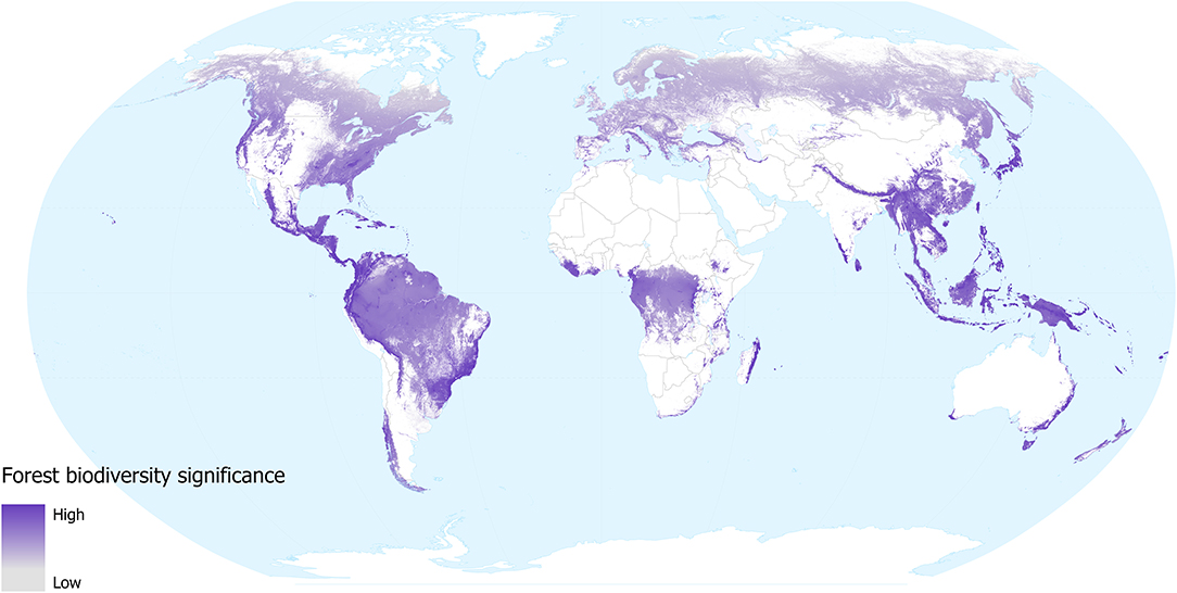
Figure 1. Forest biodiversity significance in 2018, in terms of the contribution of each location to the distributions of forest mammal, bird, amphibian, and conifer species occurring in them. Grey shows low and dark purple shows high significance values. White shows areas not classified as forest (i.e., tree cover values were <60% in 2000, lost between 2000 and 2018, or mapped as plantations).

The forest biodiversity significance of tree-cover lost from 2000 to 2018 gives an indication of the impacts of removal of forested habitat (with the caveat that some forest loss may be from natural causes, such as hurricane damage). Our results (Figure 2) highlight those regions where tree cover loss (change from above 60% tree cover to 0% tree cover within a 1 km² pixel) has resulted in disproportionate loss of the distributions of the world's forest-dependent species (in the taxonomic groups considered): Madagascar, parts of eastern Brazil, central America, SE Asia, West Africa, Australia, and northern New Zealand. Intermediate levels of loss are seen across large regions of the forests of continental and insular SE Asia. Although areas of particularly significant forest biodiversity loss occurred in the tropics during this period (a reflection of the higher species richness as well as the density of endemic species within the tropics), it should be noted that the map also highlights the biodiversity significance of the substantial extent of deforestation that has occurred over the last 18 years within temperate areas. Scandinavia, Russia, Canada and the USA have all undergone considerable losses in forest cover, mainly due to large-scale logging and fires (Curtis et al., 2018). Although these areas support relatively fewer species and these species tend to have larger global distributions, the aggregate biodiversity impacts may be substantial. The layer does not distinguish between forest loss that is likely to be permanent in the foreseeable future (e.g., conversion to agriculture) and forest loss that may only be temporary (e.g., resulting from fires or sustainable forestry practices in parts of Canada and Scandinavia). We did not consider forest gain in our assessment, but this is unlikely to overestimate biodiversity loss substantially during the period, as most forest-dependent species do not recolonise young regrowth.

FIGURE 2

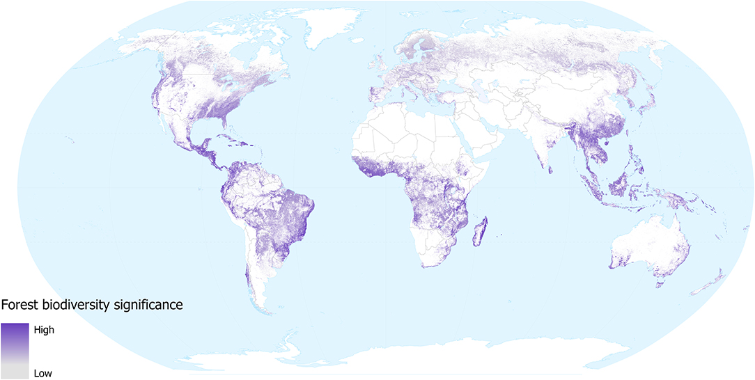
Figure 2. Forest biodiversity significance for areas of forest loss during 2000–2018, in terms of the contribution of each location to the distributions of forest mammal, bird, amphibian, and conifer species occurring in them. Values are for the year 2000 in areas where forest was subsequently lost. Grey shows low and purple shows high significance. White areas are not classified as forest in 2000 (i.e., tree cover was <25% in 2000, or area was mapped as plantation), or where forest remains in 2018 (i.e., no loss during 2000–2018).

Forest Biodiversity Intactness

The forest biodiversity intactness layer reveals the impact that forest change and human population density has had on species assemblages.

Our models revealed that land use and human population density are significant predictors of community abundance (χ² = 38.04, df = 7, p < 0.001 and χ² = 7.99, df = 1, p = 0.005, respectively). Heavily utilised areas of the world are unsurprisingly less intact (Figure 3), for instance, much of Europe and the more densely populated areas of India, North America, Bangladesh, and China. In these areas, the impact of dense human populations together with the urban and agricultural land use required to support them has led to severe losses of biodiversity intactness. Madagascar, coastal Brazil, South Africa, southern Australia, and northern Africa, are also identified as areas with striking losses in biodiversity intactness. These regions have undergone intense removal of natural forest, but retain more of their native biodiversity due to lower levels of urbanisation.

FIGURE 3

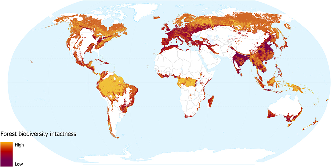
Figure 3. Forest biodiversity intactness, showing the impacts of forest change and human population density. Yellow shows more intact areas and dark red shows more degraded areas.

Comparison of Biodiversity Significance and Intactness

Overlaying biodiversity intactness and significance provides insight into areas with high values for both, and areas that score highly for one but not the other. Regions with high values for both metrics include the Northern Andes and Central America, south-eastern Brazil, the western, and eastern parts of the Congo basin, southern Japan, the Himalayas, and various parts of Southeast Asia and New Guinea (Figures 4, 5). By contrast, Europe (Figure 5D) is dominated by large areas of biodiversity intactness in the north-east and areas of high biodiversity significance in the south, but lacks large areas where both are high.

FIGURE 4

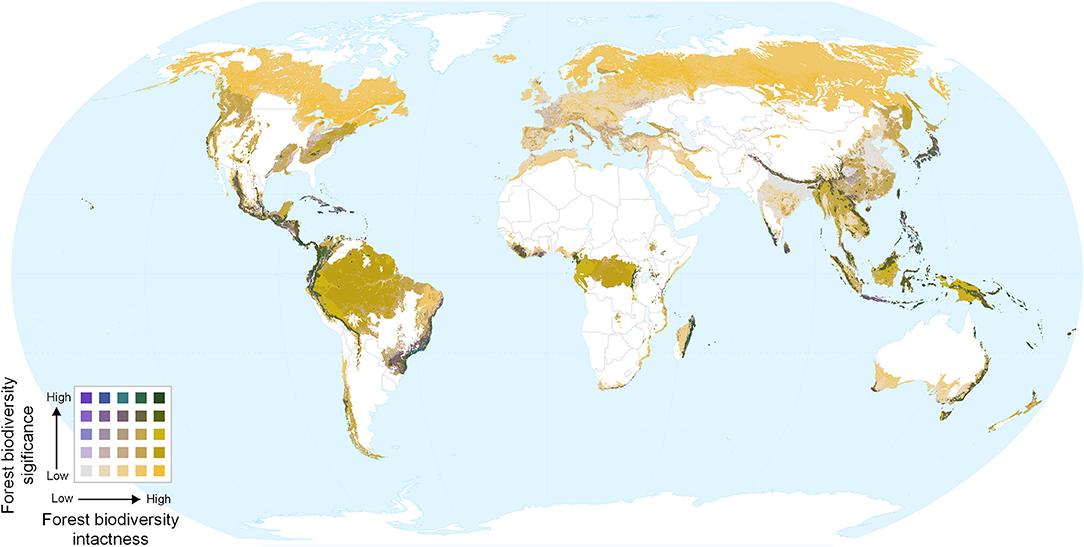
Figure 4. Bivariate map of forest biodiversity significance and intactness. Dark green areas show both high intactness and high significance.

FIGURE 5

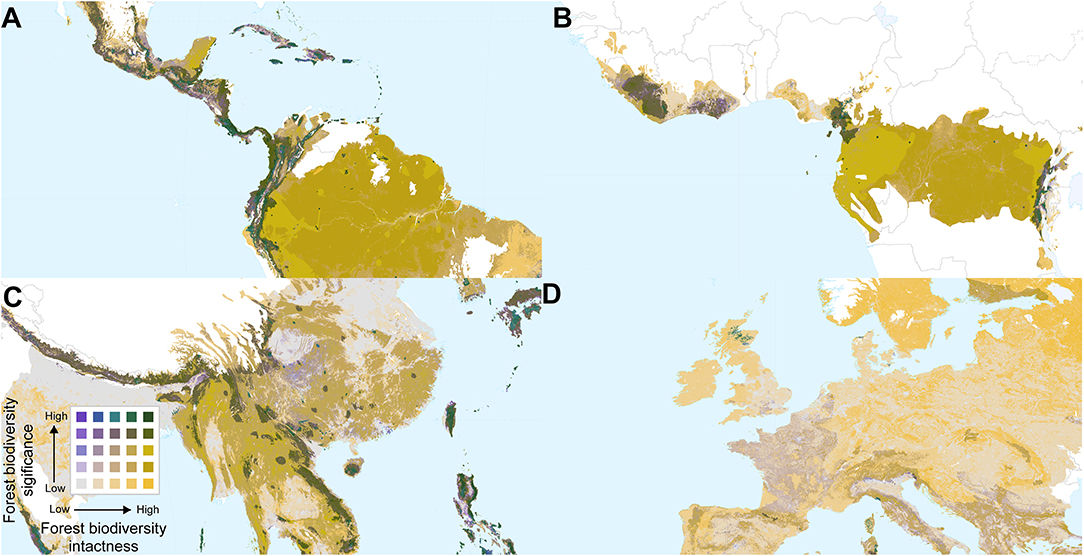
Figure 5. Bivariate maps of forest biodiversity significance and intactness within forest biomes, focused on parts of (A) Central and South America, (B) Central and West Africa, (C) China and South East Asia, and (D) Western Europe. Spatial scales differ among the panels.

Discussion

We present two new biodiversity layers for the world's forests, derived from existing data but in novel ways that aim to add contextual meaning to forest data for use in conservation decision-making.

The layers describe two different dimensions of biodiversity and so are not expected to show the same geographic patterns. Biodiversity significance combines spatial variation in both species richness and levels of endemism, and hence shows the relative contribution of any location to the persistence of forest species. However, the degree to which the values in any particular location are driven by one of these characteristics or the other cannot be determined without further analysis. Furthermore, high endemism may result from either natural endemism, human-induced geographic restriction, or a combination. By contrast with biodiversity significance, biodiversity intactness is highest where ecological assemblages remain intact, irrespective of natural macroecological variations in species diversity or endemism; intermediate values can reflect a range of combinations of reduced overall abundance and reduced compositional similarity to an intact assemblage. In general, biodiversity significance is higher within the tropics (especially in topographically heterogeneous regions) and lower in northern, boreal regions, whereas biodiversity intactness is generally low across most of Europe, India and eastern Asia and high within wilderness areas in northern European and North American forests, as well as within tropical forest cores across Central America, South America, Africa, and Asia.

Safeguarding areas of high significance is important as their loss results in a disproportionate loss of species' distributions, especially narrow-range endemics, elevating species' risk of extinction. High intactness is important to safeguard in order to (a) maintain ecosystem functioning; (b) retain community resilience against pressures such as climate change; and, in the case of forest ecosystems, (c) help mitigate climate change through greenhouse gas regulation (Steffen et al., 2015). Biodiversity intactness is also relevant to efforts to define wilderness regions, intact forest landscapes, or areas that have been described as the “last of the wild” (Potapov et al., 2008; Watson et al., 2016, 2018).

At a more local scale, comparison of the layers may provide information relevant for conservation. For example, landscapes of high significance but low intactness may be appropriate targets for restoration efforts. Landscapes that contain both high intactness and high significance reveal locations with relatively high density of geographically restricted native species. Such areas may therefore be important to safeguard through broad-scale policy responses or site-scale conservation measures such as designation of protected areas. However, biodiversity has multiple dimensions and here we have chosen to focus on just two. When considering prioritisation of areas for conservation management other aspects of biodiversity may also be relevant such as phylogenetic diversity or the presence of charismatic species.

The biodiversity significance layer shows similar patterns to those revealed by the distribution of endemic bird areas and biodiversity hotspots that were identified in the 1990s (Myers, 1990; Mittermeier et al., 1998, 2004; Stattersfield et al., 1998). The advantage of our approach is that it is based on many more species than used in these earlier analyses, and the distribution of each species considered is spatially explicit, allowing much finer resolution maps. Furthermore, the analytical approach is repeatable and allows the layer to be updated as more species and taxonomic groups are added.

The biodiversity intactness later broadly accords with Newbold et al.'s (2016) map, with areas of greatest loss in densely populated and heavily converted regions such as most of western Europe, northern China, and the southern coast of South Africa. However, our estimates for plantation-rich parts of Southeast Asia are notably lower than those of Newbold et al. (2016), which were criticized by Martin et al. (2019) as being too high. Our forest biodiversity intactness map is also able to distinguish areas of recent (post-2005) forest change, such as lowland Mexico and regions in Southeast Asia.

The outputs we highlight here are relevant to international and national policy including the Convention on Biological Diversity (CBD) (Parties' National Biodiversity Strategies and Action Plans, and National Reports), the Paris Agreement of the UN Framework Convention on Climate Change, Bonn Challenge, and global environmental assessment processes such as the Intergovernmental Science-Policy Platform on Biodiversity and Ecosystem Services and the Global Biodiversity Outlook. The layers are potentially useful both for targeting policy responses and on-ground interventions, and for tracking progress towards goals and targets. For example, global, regional and national maps and indicators of the proportion of areas of high forest biodiversity significance or intactness lost over time are relevant to Aichi Target 5 in terms of measures of loss and degradation of habitats, Aichi Target 11 in terms of areas of biodiversity significance, and Aichi Target 12 in terms of preventing extinctions and declines of threatened species. Data on tree-cover loss linked to biodiversity can also be used for national REDD+ planning and monitoring other commitments to international, regional and nation agreements, policies, and laws. The layers are also relevant to the safeguard policies of investors, financial institutions, and companies.

The data that we have brought together here are the best available, but have a number of limitations. For instance, the Hansen et al. (2013) dataset does not allow for regional calibration, yet the height and density of natural tree cover will vary depending upon local variations in environmental conditions (Tropek et al., 2014). We were not able to account for the variation of natural tree cover on a local scale and, as no standard definition of the tree cover associated with natural forests exists at larger scales, our conservative literature-based choice of a 60% tree cover threshold is unlikely to optimally delimit natural forest across the entire area of our analysis. A comparison of the biodiversity significance and intactness maps derived using a 25% tree cover threshold to indicate forest presence (SM Figures 1–3) illustrates this issue. For instance, when considering the biodiversity significance layer, landscapes with high endemicity and a naturally low forest cover are highlighted in the layer at this lower threshold, including the Okavango Delta in Botswana, the South African coast, and the western coast of Madagascar (SM Figure 1). Likewise, the biodiversity intactness layer produced using the 25% threshold reveals intactness with northern boreal forests and dry forests in Zambia, which have a naturally sparse tree cover, that are not highlighted in the 60% threshold layer. However, the 25% threshold intactness layer does not show degraded areas within West Africa, including south-east Ghana, which would naturally be covered with dense tree cover (SM Figure 3). The Hansen et al. (2013) dataset does not provide gain data across all years of our analysis, which meant that it could not be used within the biodiversity significance layer. However, this is unlikely to bias our results substantially given that forests often take considerable time before becoming suitable for forest-specialist species (Newbold et al., 2014).

When producing the biodiversity significance layer, the forest species' distribution maps were clipped by forest cover and suitable elevations to create maps of the Extent of Suitable Habitat (sensu Beresford et al., 2011), which are finer resolution representations of distribution. However, they do not map occupancy per se, and contain commission errors (e.g., owing to extirpation caused by over-exploitation, invasive alien species etc.), although this is not likely to bias the broad patterns across >12,000 species that are shown in the resulting layer. The layer does not take account of variation in abundance within species' distributions, spatial data for which are not available for the large set of species considered. The data used are not currently taxonomically representative—for instance, no invertebrates are included—and clades may have systematically different degrees of spatial resolution in their distributions resulting in the species with the most resolved maps obtaining higher values. The coding of forest dependence in the IUCN Red List does not capture finer-scale variation. In the coming years, the layer will be updated to incorporate data on the distributions of all forest reptiles and a number of forest plant groups (e.g., trees, gingers, rattans) and invertebrate taxa (e.g., dragonfly, monarch and swallowtail butterflies) as these are assessed and mapped for the IUCN Red List.

Likewise, the biodiversity intactness layer has caveats (though our analysis overcomes many of the issues raised by Martin et al., 2019; see also Newbold et al., 2019). For instance, the layer is based upon data extracted from the (Hansen et al., 2013) (updated) tree cover change dataset which only dates back to 2000. Therefore, we are not able to distinguish between forest that had recovered by 2000 and pristine forest. The biodiversity intactness layer reflects how species communities are impacted by land use change and human population density. However, we know that other anthropogenic pressures—such as climate change, hunting and exploitation—are also important, but will only be accommodated in our analysis to the extent that land use or human population density serve as proxies. Although climate change has a significant impact on biodiversity, it is not possible to disaggregate the impacts of a changing climate from the impacts of land use change and human populations over the short time period on which our analysis focuses. Roads open forest areas and affect biodiversity through harvesting (Sodhi et al., 2004), the introduction of alien species (Hulme, 2009), alterations in the microclimate and creating light gaps (Laurance et al., 2009) but these subtle changes were not captured in our analysis.

We have used the plantation data for countries where such data is available in the SDPT, but it is not possible to distinguish all plantation forests from natural forests, notably for countries not represented in the SDPT dataset. Furthermore, it should be noted that China and Papua New Guinea are present in the SDPT dataset but we were not able to obtain permission for their data to be included in this analysis. This deficiency impacts both approaches. In the forest biodiversity significance layer, plantations may wrongly appear as highly significant if the forest they replaced had high values (but not so otherwise). In the intactness layer, plantations that contained mature trees in 2000 are indistinguishable from primary or mature secondary forests, but those plantations composed of primarily non-native species or high intensity, monoculture plantations will have markedly lower intactness than indicated.

Technological revolutions over the last few years, including in our ability to obtain and process satellite-derived data with freely available supercomputer power, are opening up new areas of opportunity for conservation science. We are moving closer to near-real-time habitat and biodiversity-change products that can ingest remotely sensed data and run algorithms to show both areas of forest loss and the consequences for multiple facets of biodiversity, within time periods that can lead to rapid responses and interventions on the ground. Our work represents a further contribution to this aim.

The layers described here have been integrated into the Global Forest Watch platform (www.globalforestwatch.org), which aims to provide the data necessary to document and conserve forests worldwide. It provides information relevant to monitoring fires, documenting illegal activities, screening estates for deforestation and analysing trends in forest change.

Humanity has long relied upon forests, and the varied and complex species assemblages they encompass and support, but in recent times human impacts have become unsustainable, creating areas depauperate in biodiversity. The layers presented here help to evaluate and map how we have impacted forest biodiversity and can inform what measures can be taken at a local scale to conserve and restore forests.

Data Availability Statement

The datasets analyzed for this study can be found in the NHM data portal (data.nhm.ac.uk), and through request at www.iucnredlist.org/resources/spatial-data-download, and www.datazone.birdlife.org/species/requestdis, and the resulting layers can be visualized on the Global Forest Watch portal (data.globalforestwatch.org).

Author Contributions

SH and AA led all analyses. CM carried out analyses. SH, AA, CM, SB, CH-T, CC, CD, AP, and NB devised the methodology. All co-authors assisted in the production of the manuscript.

Funding

Funding was provided to UNEP-WCMC, IUCN, and BirdLife through World Resources Institute (WRI) Global Forest Watch. Anonymous donors, the MacArthur Foundation and the Norwegian government provided funding to WRI, with extra funding to Resolve from the Leonardo DiCaprio Fund (LDF). Funding was provided to the Natural History Museum by NERC (grant NE/M014533/1).

Conflict of Interest

The authors declare that the research was conducted in the absence of any commercial or financial relationships that could be construed as a potential conflict of interest.

Acknowledgments

We thank the GFW partnership convened by WRI for the opportunity to undertake this work, the MacArthur Foundation, anonymous donors, LDF, NERC (grant NE/M014533/1) and the Norwegian government for funding. Many people have inputted data, ideas, and expertise into the analyses that are developed and presented here: Brian O'Connor, Joe Gosling, Val Kapos, Corinna Ravilious at UNEP-WCMC, Adriana De Palma at the Natural History Museum in London, Yichuan Shi and Ackbar Joolia at IUCN, Rebecca Moore and David Thau in Google, Charlie Hofman, Brookie Gudzer-Williams and Thailynn Munroe in WRI, Alison Beresford and Graeme Buchanan in RSPB, Matt Hansen and his group in University of Maryland for providing the underlying tree cover and change layers, for their tree cover product and NASA for making Landsat data freely available. We also thank the thousands of individuals and organisations who contribute to IUCN Red List assessments, and the hundreds of people who have helped compile the PREDICTS database. Without these efforts these kinds of analyses would not be possible.

Supplementary Material

The Supplementary Material for this article can be found online at: https://www.frontiersin.org/articles/10.3389/ffgc.2019.00070/full#supplementary-material

References

ABARES (2018). Australia's State of the Forests Report. Canberra, ACT: Department of Agriculture and Water Resources, Australian Government.

Google Scholar

Beresford, A., Buchanan, G., Donald, P., Butchart, S. H. M., Fishpool, L. D. C., and Rondinini, C. (2011). Poor overlap between the distribution of Protected Areas and globally threatened birds in Africa. Anim. Conserv. 14, 99–107. doi: 10.1111/j.1469-1795.2010.00398.x

CrossRef Full Text | Google Scholar

Betts, M. G., Wolf, C., Ripple, W. J., Phalan, B., Millers, K. A., Duarte, A., et al. (2017). Global forest loss disproportionately erodes biodiversity in intact landscapes. Nature 547:441. doi: 10.1038/nature23285

PubMed Abstract | CrossRef Full Text | Google Scholar

Bird, J. P., Buchanan, G. M., Lees, A. C., Clay, R. P., Develey, P. F., Yepez, I., et al. (2012). Integrating spatially explicit habitat projections into extinction risk assessments: a reassessment of Amazonian avifauna incorporating projected deforestation. Divers. Distrib. 18, 273–281. doi: 10.1111/j.1472-4642.2011.00843.x

CrossRef Full Text | Google Scholar

BirdLife International Handbook of the Birds of the World (2016). Bird Species Distribution Maps of the World. Version 6.0. Available online at: http://datazone.birdlife.org/species/requestdis (accessed October, 2017).

Google Scholar

Brooks, T. M., Pimm, S. L., Akçakaya, R., Buchanan, G. M., Butchart, S. H. M., Foden, W., et al. (2019). Measuring Area of Habitat (AOH) and its utility for the IUCN Red List. Trends Ecol. Evol. 34, 977–986. doi: 10.1016/j.tree.2019.06.009

PubMed Abstract | CrossRef Full Text | Google Scholar

Buchanan, G. M., Butchart, S. H. M., Dutson, G., Pilgrim, J. D., Steininger, M. K., Bishop, K. D., et al. (2008). Using remote sensing to inform conservation status assessment: estimates of recent deforestation rates on New Britain and the impacts upon endemic birds. Biol. Conserv. 141, 56–66. doi: 10.1016/j.biocon.2007.08.023

CrossRef Full Text | Google Scholar

Buchanan, G. M., Donald, P. F., and Butchart, S. H. M. (2011). Identifying priority areas for conservation: a global assessment for forest-dependent birds. PLoS ONE 6:e29080. doi: 10.1371/journal.pone.0029080

PubMed Abstract | CrossRef Full Text | Google Scholar

Curtis, P. G., Slay, C. M., Harris, N. L., Tyukavina, A., and Hansen, M. C. (2018). Classifying drivers of global forest loss. Science 361, 1108–1111. doi: 10.1126/science

PubMed Abstract | CrossRef Full Text | Google Scholar

Danielson, J. J., and Gesch, D. B. (2011). Global Multi-Resolution Terrain Elevation Data 2010 (GMTED2010). Open-File Report. U.S. Geological Survey. doi: 10.3133/ofr20111073

CrossRef Full Text | Google Scholar

De Palma, A., Hoskins, A., Gonzalez, R. E., Newbold, T., Sanchez-Ortiz, K., Ferrier, S., et al. (2018). Changes in the Biodiversity Intactness Index in tropical and subtropical forest biomes, 2001-2012'. bioRxiv. doi: 10.1101/311688

CrossRef Full Text | Google Scholar

Dinerstein, E., Olson, D., Joshi, A., Vynne, C., Burgess, N. D., Wikramanayake, E., et al. (2017). An ecoregion-based approach to protecting half the terrestrial realm. Bioscience 67, 534–545. doi: 10.1093/biosci/bix014

PubMed Abstract | CrossRef Full Text | Google Scholar

FAO (2000). On Definitions of Forest and Forest Change, FRA Working Paper 33. Rome: FAO.

Google Scholar

Ficetola, G. F., Rondinini, C., Bonardi, A., Baisero, D., and Padoa-Schioppa, E. (2015). Habitat availability for amphibians and extinction threat: a global analysis. Divers. Distrib. 21, 302–311. doi: 10.1111/ddi.12296

CrossRef Full Text | Google Scholar

Foley, J. A., Defries, R., Asner, G. P., Barford, C., Bonan, G., Carpenter, S. R., et al. (2005). Global consequences of land use. Science 309, 570–574. doi: 10.1126/science.1111772

PubMed Abstract | CrossRef Full Text | Google Scholar

Gibson, L., Lee, T. M., Koh, L. P., Brook, B. W., Gardner, T. A., Barlow, J., et al. (2011). Primary forests are irreplaceable for sustaining tropical biodiversity. Nature 478:378. doi: 10.1038/nature10425

PubMed Abstract | CrossRef Full Text | Google Scholar

Gorelick, N., Hancher, M., Dixon, M., Ilyushchenko, S., Thau, D., and Moore, R. (2017). Google Earth Engine: planetary-scale geospatial analysis for everyone. Remote Sens Environ. 202, 18–27. doi: 10.1016/j.rse.2017.06.031

CrossRef Full Text | Google Scholar

Grossman, D. H., Faber-Langendon, D., Weakley, A. S., Anderson, M., Bourgeron, P., Crawford, R., et al. (1998). International Classification of Ecological Communities: Terrestrial Vegetation of the United States. Volume 1. The National Vegetation Classification System: Development, Status and Applications. Arlington, TX: The Nature Conservancy.

Google Scholar

Hansen, M. C., Potapov, P. V., Goetz, S. J., Turubanova, S., Tyukavina, A., Krylov, A., et al. (2016). Mapping tree height distributions in Sub-Saharan Africa using Landsat 7 and 8 data. Remote Sens. Environ. 185, 221–232. doi: 10.1016/j.rse.2016.02.023

CrossRef Full Text | Google Scholar

Hansen, M. C., Potapov, P. V., Moore, R., Hancher, M., Turubanova, S. A., Tyukavina, A., et al. (2013). High-resolution global maps of 21st-century forest cover change. Science 342:850. doi: 10.1126/science.1244693

PubMed Abstract | CrossRef Full Text | Google Scholar

Hansen, M. C., Stehman, S. V., and Potapov, P. V. (2010). Quantification of global forest cover loss Proc. Natl. Acad. Sci. U.S.A. 107, 8650–8655. doi: 10.1073/pnas.0912668107

PubMed Abstract | CrossRef Full Text | Google Scholar

Harris, N. L., Goldman, E. D., and Gibbes, S. (2019). Spatial Database of Planted Trees Version 1.0.” Technical Note. Washington, DC: World Resources Institute. Available online at: https://www.wri.org/publication/spatialdatabase-planted-trees (accessed May, 2019).

Google Scholar

Hoskins, A. J., Bush, A., Gilmore, J., Harwood, T., Hudson, L. N., Ware, C., et al. (2016). Downscaling land-use data to provide global 30″ estimates of five landuse classes. Ecol. Evol. 6, 3040–3055. doi: 10.1002/ece3.2104

CrossRef Full Text | Google Scholar

Hudson, L. N., Newbold, T., Contu, S., Hill, S. L. L., Lysenko, I., De Palma, A., et al. (2017). The database of the PREDICTS (Projecting Responses of Ecological Diversity In Changing Terrestrial Systems) project. Ecol. Evol. 7, 145–188. doi: 10.1002/ece3.2579

PubMed Abstract | CrossRef Full Text | Google Scholar

Hulme, P. E. (2009). Trade, transport and trouble: managing invasive species pathways in an era of globalization. J. Appl. Ecol. 46, 10–18. doi: 10.1111/j.1365-2664.2008.01600.x

CrossRef Full Text | Google Scholar

IUCN (2017). The IUCN Red List of Threatened Species, Version 2017-2. IUCN. Available online at: http://www.iucnredlist.org

Google Scholar

Klein Goldewijk, K., Beusen, A., de Vos, M., and van Drecht, G. (2011). The HYDE 3.1 spatially explicit database of human induced land use change over the past 12,000 years. Glob. Ecol. Biogeogr. 20, 73–86. doi: 10.1111/j.1466-8238.2010.00587.x

CrossRef Full Text | Google Scholar

Kohl, M., and Päivinen, R. (1996). Definition of a System of Nomenclature for Mapping European Forests and for Compiling a Pan-European Forest Information System. Luxembourg: Space Applications Institute of the Joint Research Centre and the European Forest Institute; Office for Official Publications of the European Communities.

Google Scholar

Laurance, W. F., Goosem, M., and Laurance, S. G. W. (2009). Impacts of roads and linear clearings on tropical forests. Trends Ecol. Evol. 24, 659–669. doi: 10.1016/j.tree.2009.06.009

PubMed Abstract | CrossRef Full Text | Google Scholar

Lund, H. G. (2002). When is a forest not a forest? J. For. 100, 21–28. doi: 10.1353/vcr.2002.0025

CrossRef Full Text | Google Scholar

Lund, H. G. (2015). Sure, We Can All Agree We Should Protect Our Forests. But Can We Agree on What IS a Forest? Gainesville, VA: Forest Information Services

Google Scholar

Magdon, P., Fischer, C., Fuchs, H., and Kleinn, C. (2014). Translating criteria of international forest definitions into remote sensing image analysis. Remote Sens. Environ. 149, 252–262. doi: 10.1016/j.rse.2014.03.033

CrossRef Full Text | Google Scholar

Magdon, P., and Kleinn, C. (2013). Uncertainties of forest area estimates caused by the minimum crown cover criterion. Environ. Monit. Assess. 185:5345. doi: 10.1007/s10661-012-2950-0

PubMed Abstract | CrossRef Full Text | Google Scholar

Magugu, R., and Chitiga, M. (2002). Accounting for Forest Resources in Zimbabwe. CEEPA Discussion Paper No 7, CEEPA, University of Pretoria.

Google Scholar

Martin, P. A., Green, R. E., and Balmford, A. (2019). The biodiversity intactness index may underestimate losses. Nat. Ecol. Evol. 3, 862–863. doi: 10.1038/s41559-019-0895-1

PubMed Abstract | CrossRef Full Text | Google Scholar

Mittermeier, R. A., Gil, P. R., Hoffman, M., Pilgrim, J., Brooks, T., Mittermeier, C. G., et al. (2004). Hotspots Revisted. Earth's Biologically Richest and Most Endangered Terrestrial Ecoregions. Mexico City: Cemex

Google Scholar

Mittermeier, R. A., Myers, N., Thomsen, J. B., da Fonseca, G. A. B., and Olivieri, S. (1998). Biodiversity hotspots and major tropical wilderness areas: approaches to setting conservation priorities. Conserv. Biol. 12, 516–520. doi: 10.1046/j.1523-1739.1998.012003516.x

CrossRef Full Text | Google Scholar

Myers, N. (1990). The biodiversity challenge: expanded hot-spots analysis. Environmentalist 10, 243–256. doi: 10.1007/BF02239720

PubMed Abstract | CrossRef Full Text | Google Scholar

Newbold, T., Hudson, L. N., Arnell, A. P., Contu, S., De Palma, A., Ferrier, S., et al. (2016). Has land use pushed terrestrial biodiversity beyond the planetary boundary? A global assessment. Science 353:288. doi: 10.1126/science.aaf2201

PubMed Abstract | CrossRef Full Text | Google Scholar

Newbold, T., Hudson, L. N., Hill, S. L. L., Contu, S., Lysenko, I., Senior, R. A., et al. (2015). Global effects of land use on local terrestrial biodiversity. Nature 520, 45–50. doi: 10.1038/nature14324

PubMed Abstract | CrossRef Full Text | Google Scholar

Newbold, T., Hudson, L. N., Phillips, H. R. P., Hill, S. L. L., Contu, S., Lysenko, I., et al. (2014). A global model of the response of tropical and sub-tropical forest biodiversity to anthropogenic pressures. Proc. R. Soc. B 281:20141371. doi: 10.1098/rspb.2014.1371

PubMed Abstract | CrossRef Full Text | Google Scholar

Newbold, T., Sanchez-Ortiz, K., De Palma, A., Hill, S. L. L., and Purvis, A. (2019). Reply to ‘The biodiversity intactness index may underestimate losses’. Nat. Ecol. Evol. 3, 864–865. doi: 10.1038/s41559-019-0896-0

PubMed Abstract | CrossRef Full Text | Google Scholar

Newbold, T., Scharlemann, J. P. W., Butchart, S. H. M., Sekercioglu, Ç. H., Alkemade, R., Booth, H., et al. (2013). Ecological traits affect the response of tropical forest bird species to land-use intensity. Proc. R. Soc. B Biol. Sci. 280:20122131. doi: 10.1098/rspb.2012.2131

PubMed Abstract | CrossRef Full Text | Google Scholar

Olson, D., Dinerstein, E., Wikramanayake, E., Burgess, N., Powell, G., Underwood, E., et al. (2001). Terrestrial ecoregions of the worlds: a new map of life on Earth. Bioscience 51, 933–938. doi: 10.1641/0006-3568(2001)051[0933:TEOTWA]2.0.CO;2

CrossRef Full Text | Google Scholar

Phillips, H. R. P., Newbold, T., and Purvis, A. (2017). Land-use effects on local biodiversity in tropical forests vary between continents. Biodivers. Conserv. 26, 2251–2270. doi: 10.1007/s10531-017-1356-2

CrossRef Full Text | Google Scholar

Potapov, P., Yaroshenko, A., Turubanova, S., Dubinin, M., Laestadius, L., Thies, C., et al. (2008). Mapping the world's intact forest landscapes by remote sensing. Ecol. Soc. 13:51. doi: 10.5751/ES-02670-130251

CrossRef Full Text | Google Scholar

Purvis, A., Newbold, T., De Palma, A., Contu, S., Hill, S. L. L., Sanchez-Ortiz, K., et al. (2018). “Chapter five - modelling and projecting the response of local terrestrial biodiversity worldwide to land use and related pressures: the PREDICTS project,” in Advances in Ecological Research, eds D. A. Bohan, A. J. Dumbrell, G. Woodward, and M. Jackson (London: Academic Press), 201–241. doi: 10.1016/bs.aecr.2017.12.003

CrossRef Full Text | Google Scholar

Rondinini, C., Di Marco, M., Chiozza, F., Santulli, G., Baisero, D., Visconti, P., et al. (2011). Global habitat suitability models of terrestrial mammals. Philos. Trans. R. Soc. B Biol. Sci. 366:2633. doi: 10.1098/rstb.2011.0113

PubMed Abstract | CrossRef Full Text | Google Scholar

Sandvoss, M., McClymont, B., and Farnden, C. (2005). A User's Guide to the Vegetation Resources Inventory. Vancouver, BC: Timberline Forest Inventory Consultants Ltd.

Google Scholar

Sodhi, N. S., Koh, L. P., Brook, B. W., and Ng, P. K. L. (2004). Southeast Asian biodiversity: an impending disaster. Trends Ecol. Evol. 19, 654–660. doi: 10.1016/j.tree.2004.09.006

PubMed Abstract | CrossRef Full Text | Google Scholar

Song, X.-P., Hansen, M. C., Stehman, S. V., Potapov, P. V., Tyukavina, A., Vermote, E. F., et al. (2018). Global land change from 1982 to 2016. Nature 560, 639–643. doi: 10.1038/s41586-018-0411-9

PubMed Abstract | CrossRef Full Text | Google Scholar

Stattersfield, A. J., Crosby, M. J., Long, A. J., and Wege, D. C. (1998). Endemic Bird Areas of the World: Priorities for Biodiversity Conservation. Cambridge, UK: BirdLife International.

Google Scholar

Steffen, W., Richardson, K., Rockström, J., Cornell, S. E., Fetzer, I., Bennett, E. M., et al. (2015). Planetary boundaries: guiding human development on a changing planet. Science 347:1259855. doi: 10.1126/science.1259855

PubMed Abstract | CrossRef Full Text | Google Scholar

Tracewski, Ł., Butchart, S. H. M., Di Marco, M., Ficetola, G. F., Rondinini, C., Symes, A., et al. (2016). Toward quantification of the impact of 21st-century deforestation on the extinction risk of terrestrial vertebrates. Conserv. Biol. 30, 1070–1079. doi: 10.1111/cobi.12715

PubMed Abstract | CrossRef Full Text | Google Scholar

Tropek, R., Sedlácek, O., Beck, J., Keil, P., Musilová, Z., Símová, I., et al. (2014). Comment on “High-resolution global maps of 21st-century forest cover change”. Science 344:981. doi: 10.1126/science.1248753

PubMed Abstract | CrossRef Full Text | Google Scholar

Tyukavina, A., Baccini, A., Hansen, M. C., Potapov, P. V., Stehman, S. V., Houghton, R. A., et al. (2015). Aboveground carbon loss in natural and managed tropical forests from 2000 to 2012. Environ. Res. Lett. 10:074002. doi: 10.1088/1748-9326/10/7/074002

CrossRef Full Text | Google Scholar

UNEP (2001). An Assessment of the Status of the World's Remaining Closed Forests. UNEP/DEWA/TR 01-2. Nairobi: UNEP.

Google Scholar

USGS Land Cover Institute (2017). Tree Cover for 2010. Available online at: https://landcover.usgs.gov/glc/TreeCoverDescriptionAndDownloads.php (accessed August, 2017).

PubMed Abstract | Google Scholar

Watson, J. E., Shanahan, M., Danielle, F., Di Marco, M., Allan, J., Laurance, W. F., et al. (2016). Catastrophic declines in wilderness areas undermine global environment targets. Curr. Biol. 26, 2929–2934. doi: 10.1016/j.cub.2016.08.049

PubMed Abstract | CrossRef Full Text | Google Scholar

Watson, J. E. M., Venter, O., Lee, J., Jones, K. R., Robinson, J. G., Possingham, H. P., et al. (2018). Protect the last of the wild. Nature 7729, 27–30. doi: 10.1038/d41586-018-07183-6

CrossRef Full Text | Google Scholar

Williams, P., Gibbons, D., Margules, C., Rebelo, A., Humphries, C., and Pressey, R. L. (1996). A comparison of richness hotspots, rarity hotspots and complementary areas for conserving diversity using British birds. Conserv. Biol. 10, 155–174. doi: 10.1046/j.1523-1739.1996.10010155.x

CrossRef Full Text | Google Scholar