A New Field Protocol for Monitoring Forest Degradation

Introduction

The world’s forests are undergoing rapid and widespread changes (Lewis et al., 2015), therefore it is vital to collect suitable empirical data to monitor these changes. Deforestation – the clearance of forest and conversion to another land use – is reasonably well understood and monitored. Long term datasets are provided by the FAO’s Forest Resource Assessments, produced every 5 years since 1980 (e.g., FAO, 2010, 2015), and independent satellite-based programs such as Global Forest Watch (Global Forest Watch, 2014) disseminate annual 30 m resolution deforestation data from Hansen et al. (2013). However, forest degradation – the removal of trees causing a reduction in Aboveground Biomass (AGB) and ecosystem services within forested land – is still very poorly quantified. There is wide disagreement on the area of forest impacted annually, including an order of magnitude uncertainty in the annual amount of carbon released (Bustamante et al., 2016; Baccini et al., 2017; De Andrade et al., 2017; McNicol et al., 2018; Mitchard, 2018).

Improving our knowledge of both the rate and extent of forest degradation is now a pressing issue. Some estimates suggest that up to 70% of tropical forest carbon emission could be coming from degradation (Baccini et al., 2017), and the area affected by degradation annually is up to 10 times greater than the area affected by deforestation (Herold et al., 2011), however, these estimates have very large uncertainties (Mitchard, 2018; Bullock et al., 2020). At a regional scale, recent estimates across the Amazon basin suggest that since 1995 the land area effected by degradation was the same as that affected by deforestation (Bullock et al., 2020). Degraded landscapes are also at the forefront of land use change, with degradation often a precursor to deforestation (Pinheiro et al., 2016), making it important to understand where this phenomena is happening. Furthermore, under the United Nations Framework Convention on Climate Change (UNFCCC) countries are now required to report emissions from forest degradation (UNFCCC, 2009; Pistorius, 2012; UNFCCC, 2015; Mitchell et al., 2017), meaning that suitable methods for estimated both the area and carbon released from degradation are essential.

Forest degradation is a much more challenging process to understand than deforestation for a number of reasons. Firstly there are many types of degradation, each with their own associated changes in carbon and ecosystem services, from very minimally disturbed forest (e.g., removal of small trees for fuelwood) to very heavily disturbed forest (e.g., industrialised selective logging which removes large trees through the use of bulldozers and leaves large skid trails, Vásquez-Grandón et al., 2018). Secondly, forest degradation is a gradual process, with repeated degradation events possible on the same piece of land. Thirdly, many degradation processes occur at very small spatial scales and are very spatially heterogeneous (Pinheiro et al., 2016). Therefore degradation has both spatial and temporal dynamics which need to be quantified (Ghazoul et al., 2015). Finally, forest degradation can be a sub-canopy process (e.g., clearance of understory trees for agricultural production), and thus effectively invisible to most Earth Observation data, and even potentially to conventional forest inventories which may only measure larger trees (typically > 10 cm diameter).

Such complexities in the causes and severity of forest degradation make it a difficult process to even define (Vásquez-Grandón et al., 2018). Indeed it has been suggested that there are over 50 working definitions of degradation (Simula, 2009), including those used by many international organisations, including the Intergovernmental Panel on Climate Change (IPCC), the Food and Agricultural Organisation (FAO), and the United Nations Environment Programme (UNEP; Sasaki and Putz, 2009). These varying definitions reflect differences in ecological characteristics as well as differences in objectives for monitoring and policy making (Ghazoul et al., 2015). The recent Methods and Guidance from the Global Forest Observations Initiative (FAO, 2020) states that ‘for reporting on REDD+, carbon stock is the primary value under consideration, so degradation is interpreted as processes leading to long term loss of carbon without land use change’. Therefore, whilst some more recent definitions only consider changes in carbon stocks as measures of degradation, there are also important considerations regarding changes in biodiversity that can result from degradation.

The relatively subtle changes in forest structure associated with degradation make it particularly challenging process to monitor and quantify using remote sensing. Traditional optical remote sensing techniques are often not suitable; understory forest clearance cannot be observed from satellites. Canopy openings following selective logging are challenging to detect, and do not persist for long periods, meaning the time window for detection is short (or non-existent if cloud cover persists over that period). These issues with remote sensing establish the need for ground based data to monitor forest degradation (Herold et al., 2011), either as a sole data source, or at minimum as a trusted ground truth for developing and testing more complex, active, remote sensing methodologies.

Forest plot networks, which use permanent sample plots (PSPs), are a well-established method for monitoring long-term changes in forest dynamics, such as carbon source and sink dynamics (Lewis et al., 2013; Brienen et al., 2015), responses to drought (Fauset et al., 2012), changes in species composition (Sullivan et al., 2017) and the effects of climate change (Esquivel-Muelbert et al., 2019). Furthermore, PSPs are vital for calibration and validation of remote sensing products, which are needed for monitoring forest changes at larger spatial scales (Chave et al., 2019). Due to the gradual nature of forest degradation, PSPs are the only means of monitoring changes on the ground accurately as losses of individual trees need to be observed. There are well-established field protocols for establishing plot networks, such as the Rainfor (Phillips et al., 2009) and ForestGEO protocols (Condit, 1998), and databases for storing and automating the processing of such data, such as the ForestPlots.net database (Lopez-Gonzalez et al., 2011). These methods have successfully been used to set up large plots networks across the globe, e.g., ForestPlots.net archives nearly 3500 plots, across 53 countries, from which thousands of scientific papers have been developed.

However, whilst these existing field protocols have yielded many important findings, they have limitations, which mean they are not ideally suited for monitoring degradation. Firstly, many existing PSP protocols focus on intact or protected forest rather than disturbed forest, meaning that many existing plots are not in suitable locations for monitoring degradation (Condit, 1998). Furthermore, it is often the case that if plots that were established in intact forest undergo disturbance, then they are excluded from future census as they are no longer useful for studying undisturbed forest (e.g., Lewis et al., 2009). However, these disturbed plots are critically required within networks to understand degradation. Secondly, the permanent marking of trees can be a deterrent to the normal behaviour of people living in and utilising forest resources (Campbell et al., 2011). To have an unbiased assessment of degradation requires no alteration in the way people or industry use the forest. Thirdly, standard 1 ha plots are demanding to set up and remeasure, estimated at approximately 22 person days per plot to lay out a plot then measure, paint, and tag all the trees. Further, if botanical samples need to be collected to establish a full tree species information, a single plot can take up to 48 person days to be measured (Phillips et al., 2009). As degradation only occurs over a small proportion of a forest area in any one year (rather than over a large or entire area as with deforestation or as the response of forests to climate change), plot networks need a high density of plots to reliably capture some degradation events. Thus for a given budget, a quicker, less demanding protocol would allow a larger area of forest to be sampled and monitored for degradation events.

An additional consideration when monitoring forest degradation is the placement of forest plots. Typically, field protocols encourage randomly distributing forest plots across the landscape (e.g., Phillips et al., 2009). However, in the case of forest degradation this may not be appropriate. For example, if you had a forest area of 2500 ha, of which 5% was degraded between two census intervals, which represents a high rate of degradation (125 ha degraded in total), and you were able to establish 10 × 1 ha plots (due to budgetary and time constraints), then just 0.4% of the forest area would be sampled. If these plots were randomly located across the landscape, the likelihood of degradation going undetected, would be high, as approximately 60% [probability of not encountering degradation = 1-(1-0.05)¹⁰ = 0.40]. Moreover, it is rather unlikely that a field campaign could sample even 0.4% of a forest area if larger than our theoretical example. For example, the Mexican National Forest Inventory (NFI), has extensive coverage with 26,220 plots covering 4,200 ha, however, this only covers 0.01% the total forest area in Mexico (CONAFOR, 2015). It might be thought that this problem could only be solved through just increasing the number of plots, or going straight to remote sensing: but this is not the case as the distribution of forest degradation across the landscape is not random. Higher instances of degradation are seen in closer proximity to access points such as along forest edges or roads (Chaplin-Kramer et al., 2015; Brinck et al., 2017). Indeed, the presence of logging roads has been used as a proxy for forest degradation (Bryan et al., 2013). Therefore, the low probability of encountering forest degradation if using a traditional field protocol that employs a random plot design, alongside the non-random distribution of degradation events, suggests that plots used to monitor forest degradation should be located non-randomly across the landscape. Such plots to monitor forest degradation should have sampling biased toward areas at higher risk of degradation, to increase the chances that a plot is degraded for a given number of plots.

Locating degradation plots non-randomly can help to detect degradation within an area. However, the challenges of estimating the level of degradation and scaling this to the landscape remain. There are a number of potential solutions. Firstly, such plots could be used as an indicator, simply to detect the unequivocal presence or absence of degradation in an area, rather than to estimate actual percentage or carbon stock change rates of forest degradation. Secondly, a simple stratification of the forest based on distance from access points (e.g., along roads or forest edges, Chaplin-Kramer et al., 2015), with more intensive sampling carried out closer to access points where there is a higher likelihood of degradation, could be used to scale up rates of change between high and low risk areas. And thirdly, the change in these field plots could be used to train remote sensing based mapping of forest degradation, which can then scale across the landscape: unlike when using normal plots for training, the higher percentage chance of having degradation events in the plots makes these plots more useful for training and testing remote sensing change algorithms.

To address this need for a forest PSP protocol specifically designed for monitoring forest degradation we created the ‘Forest Degradation Permanent Sample Plot Protocol’ (hereafter Degradation PSP Protocol), which we trialled in a forest area undergoing degradation in Jalisco State, Mexico. Here we describe this protocol and present findings from our demonstration plot network.

Methods

Protocol Design Overview

The full protocol is included in the Supplementary Information, and the justification for decisions made is described in the following section. For ease, we describe the protocol in brief here:

The aim of the “Degradation PSP protocol” is to accurately quantify ground level temporal changes in AGB and forest structure following degradation and to identify the mode of degradation. Thus, this protocol uses PSPs, rather than single census plot data, which allows individual trees to be followed through time to (1) estimate AGB in census 2 as a function of census 1, and (2) identify any individuals that died between census 1 and 2 and determine the cause of mortality. We define degradation as; “The loss of AGB due to anthropogenic disturbance from an area defined as forest, that remains as forest after the disturbance,” therefore we principally consider changes in AGB, however, the protocol we present could be applied more broadly to assess changes in biodiversity as well. Permanent sample plots are established in forested areas currently undergoing degradation or under pressure from degradation. The location of plots should follow a selective sampling approach, with areas closer to sources of disturbance that have a higher risk of degradation having a larger number of plots (Figure 1 and explained in detail in “Sample Design and Plot Layout” section below).

FIGURE 1

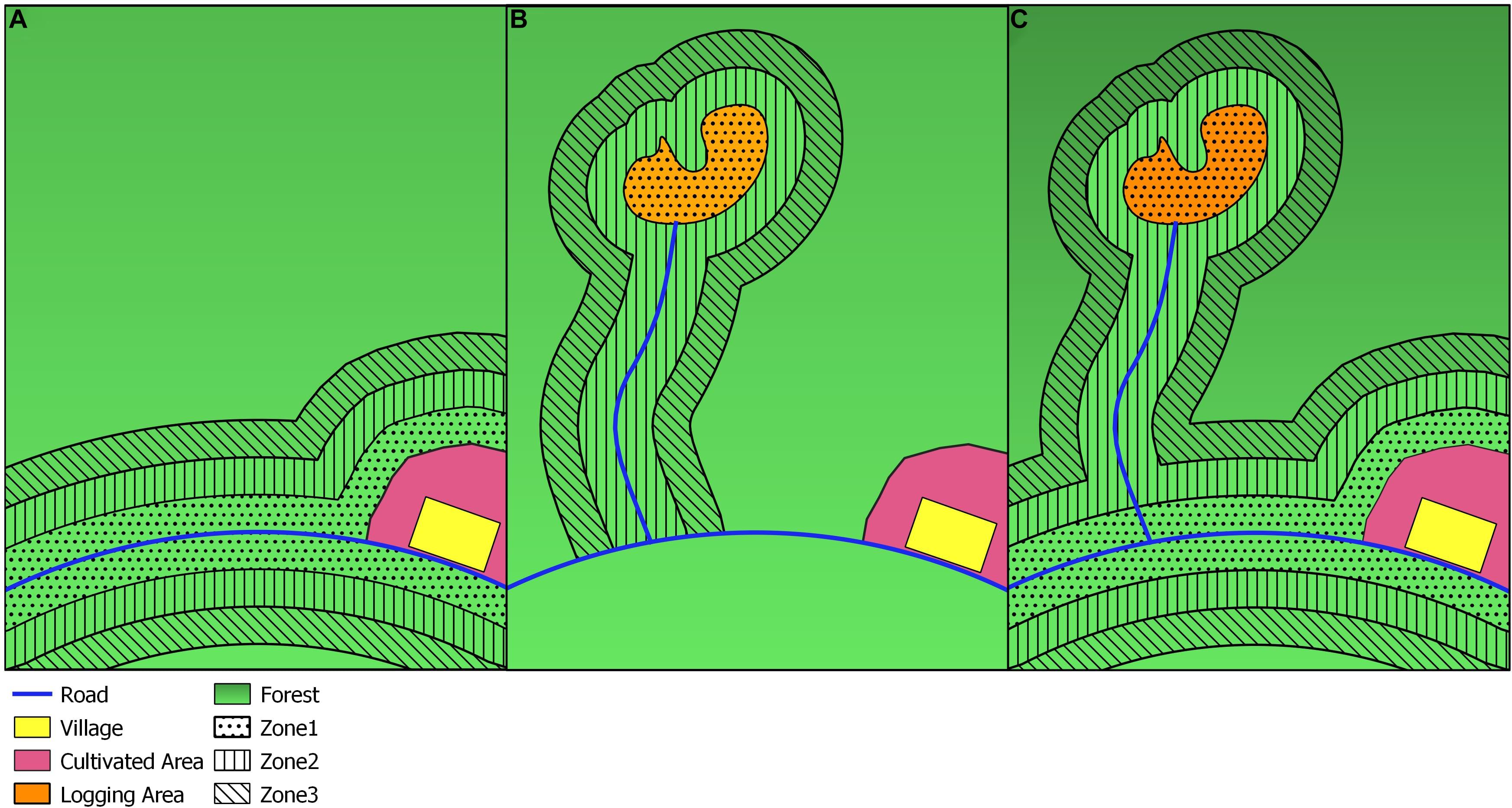
Figure 1. Diagram of stratified sampling design, showing sampling zone 1 (points), zone 2 (vertical hash), and zone 3 (diagonal hash). Sampling intensity decreases from zone 1 to zone 3. (A) Degradation risk stratification – showing higher sampling along road and close to community where there is a higher risk of degradation. (B) Local Knowledge stratification – showing higher sampling within logging area, along logging access road and surrounding logging area. (C) Combination stratification – using a combination of strategy A and B to stratify sample area.

The degradation PSP protocol uses a long narrow (25 m × 200 m) transect style plot of 0.5ha, consisting of 20 sub-plots (12.5 m × 20 m; Figure 2A). Once the start point of a plot is decided, a 200 m transect line is laid out along the centre of the plot. Two sub-plots are measured every 20 m along the plot, one sub-plot to the left of the central line (0 m to 12.5 m) and one sub-plot to the right of the central line (12.5 m to 25 m; Figure 2A). GPS coordinates should be collected at every plot corner and every 20 m along the central line to aid in relocation of the plot in subsequent census (Figure 2A).

FIGURE 2

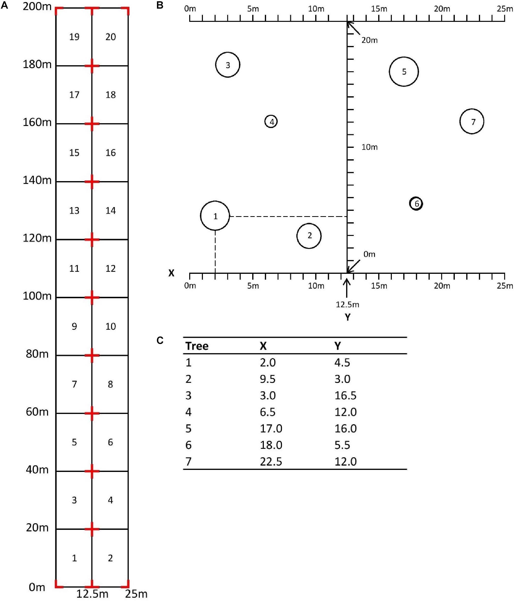
Figure 2. (A). Degradation plot layout, with sub-plot numbers inside boxes. Red crosses show location of points where GPS data should be collected. (B). Diagram explaining how to record XY coordinates of individuals in sub-plots. Dashed line shows point where XY coordinate should be taken (at centre of trunk). (C). Table shows XY Coordinates for trees 1–7 in diagram.

For each individual within a plot the following information must be collected; diameter at breast height (DBH), height, XY coordinates, species ID, condition of stem, e.g., anthropogenic or other damage to stems, such as snapped stems. Data collected in plots is used to estimate changes in AGB between census intervals. The measurement of irregular trees (e.g., trees with buttress roots, deformities, leaning or multi-stemmed trees) follows the conventions of the Rainfor protocol (Phillips et al., 2009) for consistency with other PSP networks and is describe in the Supplementary Information. XY coordinates are measured to the centre of the trunk to the nearest 10cm (Figures 2B,C).

Protocol Rational

Criteria for Plot Establishment

To ensure degradation events are captured the criteria for plot establishment is different to standard scientific forest inventory plots (which are typically large and square/circular to reduce edge effects, with permanently marked trees, and away from potential human disturbance). In this protocol we have moved away from these conventions for the following reasons:

1. Due to the heterogeneous and non-random distribution of degradation events, using a fully randomised sample design is inappropriate for this protocol. Rather, for plot networks to detect degradation, they must be deliberately biased toward areas at higher risk of degradation. Therefore, plots are located in areas likely to undergo or actively undergoing anthropogenic disturbance. This includes all the potential drivers of degradation operating in the region in question, e.g., selective logging of timber, clearing of trees for fuelwood, removal of sub-canopy trees for agricultural expansion (such as shade grown coffee or cacao), harvesting of non-timber forest products, or slash and burn agriculture. Typically such activities take place nearer to villages, agricultural areas, roads or paths, therefore, the degradation PSP protocol uses a selective sampling arpproach with a higher number of plots located closer to likely sources of disturbance (see ‘Sample Design and Plot Layout’).

2. Plots must be quick to measure. The reasons for speed being critical are two-fold:

(a) Due to the spatial heterogeneity of forest degradation, it is unlikely that each individual plot will be disturbed within a census interval. Thus, it is important to establish a large number of plots so a reasonable number may be disturbed. Ideally, a field team should be able to create 1–2 plots per day, or between 20 and 40 plots per month, once accounting for breaks and travelling.

(b) The presence of researchers and field teams within a plot for a number of days may reduce the likelihood of local people entering the area and conducting degrading activities as normal. Data collection should not lead to any bias in land use or harvesting activities.

3. Stems in plots must not be permanently marked or tagged (for the same reason explained in 2.b), but it must be possible to relocate each stem, so individuals can be tracked through time. For this reason, trees must be carefully located and mapped so individuals can be relocated in any subsequent census.

4. Plots must be large enough to be useful for calibration and validation of earth observation data (typically at least 0.5 ha) and to provide unbiased AGB estimates (e.g., Mitchard et al., 2011). Remote sensing is essential for mapping the extent of forest degradation, therefore, any field protocol must ensure plots have the dual purpose of monitoring changes on the ground and calibrating earth observation data (Chave et al., 2019).

Sample Design and Plot Layout

Within areas under threat of degradation, there are several land use transitions that could occur between census 1 and census 2, and researches will not know what transition will take place a priori (Table 1). For example, if a plot is undisturbed in census 1, it either could have been left undisturbed or have undergone degradation by census 2. As the aim of this protocol, it to quantify ground level changed resulting from degradation it is necessary to bias sampling toward areas at higher risk of degradation to increase the likelihood of capturing degradation within the PSP network. To fulfil this objective the Degradation PSP protocol uses a selective sampling strategy with a larger number of plots located in areas at higher risk of degradation. Traditional selective sampling strategies, where researchers locate plots based on knowledge of the area, suffer from a lack of randomness (Speak et al., 2018). Therefore, we incorporate stratification into the sampling strategy to introduce randomness (Michalcová et al., 2011).

TABLE 1

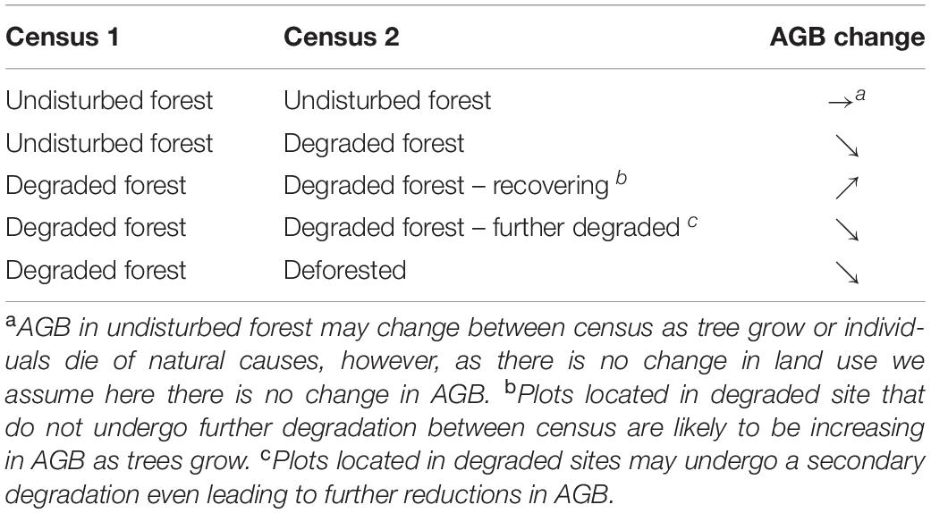
Table 1. Possible land use transitions between census 1 and census 2 and the direction of change in AGB between census, within landscapes that are undergoing degradation or are under threat of degradation Flat arrow = no change in AGB, downward arrow = decreasing AGB, upward arrow = increasing AGB.

Stratification is done by creating buffer zones around areas either (1) undergoing or (2) at risk of degradation. Within each strata, plots should be randomly distributed. Stratification in areas undergoing degradation is based on local knowledge of an area, and where degradation is known to be underway. A higher number of plots are located in core areas where degradation is underway, as the distance from areas undergoing degradation increased the number of plots decreased. Whereas stratification around areas at risk of degradation is determined by the proximity to access points such as; roads, forest edges, or distance to communities. A higher number of plots are located in areas immediately adjacent to access points, as the distance to access points increased the number of plots decreased (Figure 1). Conceptually, the sampling strategy proposed here is similar to a full-stratified random sample; however, it is not based on prior knowledge of the observed variance among strata, but rather is based on the knowledge of researchers and the likelihood of degradation taking place. Whilst a selective sampling strategy reduces the ability to make statistical inferences from the data, it enables you to capture the phenomena of interest (here degradation) more thoroughly (Michalcová et al., 2011).

This protocol uses a long narrow plot (Figure 2A), which helps reduce the time needed for plot measurement as field teams can move along the plot (laying out and measuring sub-plots) as they collect data, and remove any markers as they go. This shape of plot has been widely used in logging sites in parts of Africa (Cameroon, Central African Republic, and Republic of Congo; Fayolle et al., 2012; Ouédraogo et al., 2016), and has been used successfully to ground truth remote sensing products for mapping AGB (Mitchard et al., 2011) and therefore is appropriate for use in degraded tropical forest. Long narrow plots do have increase edge compared to equivalent sized square plots; however, by tracking individual stems through time using XY coordinates and making careful decisions as to whether trees are “in” or “out,” the impacts of increased edge are mitigated. We do not doubt that square plots would produce slightly more reliable estimates of AGB (due to lower edge effects) and would be better for matching to remote sensing pixels, however, those benefits do not, we believe, outweigh the costs of the additional time needed to set up the plots.

Diameter

As a minimum, all stems ≥10 cm DBH should be measured at 1.3 m. The minimum DBH should be set based on local conditions; in forests that store a higher proportion of AGB in smaller stems the minimum DBH threshold should be lower. For example, in the tropical dry forests of the Yucatan peninsula, Mexico, >30% of AGB is found in stems <10 cm DBH; in disturbed forests the AGB in small stems can increase to 80% of total AGB (Read and Lawrence, 2003; Romero-Duque et al., 2007), therefore a minimum DBH of 5cm DBH would be more appropriate. Furthermore the type of degradation should be considered when deciding on a minimum DBH, processes such as selective logging primarily target large trees >50 cm DBH (Peña-Claros et al., 2008), whereas other processes such as fuelwood extraction focus on smaller stems (Pote et al., 2006). Understanding of local pressures is important to ensure degrading activities are captured within PSP networks.

Height

Whenever possible the height of all stems should be measured, as degradation causes disturbances which may not results in the complete removal of an individual stem. For example, selective logging can cause substantial damage to the residual forest stand; Matangaran et al. (2019) found that following selective logging in Indonesia up to 31% of residual stand damage was from broken stems. Broken stems may not be immediately committed to mortality; however, changes in stem height must be measured to estimate the AGB contained in the downed portion of the stem as this represents committed future emissions (Ribeiro et al., 2016). Whenever possible the height of all trees should be measured, because we specifically expect negative changes in tree heights to be part of the degradation signal. Note, this is different to the scientific inventory approaches (e.g., Rainfor, Phillips et al., 2009), where it is acceptable to use DBH and species only (relying on DBH:height allometric equations to estimate height), or measure a subset of stems and develop a local DBH:height relationship. However, in some instances we accept that measuring height of all trees may not be possible. In these cases a subset of trees that cover the full range of DBH values should be measured and a locally derived DBH:height allometry should be developed (see Supplementary Information).

Identifying Mode of Degradation

To identify the mode of degradation within plots every stem is given a tree code, which gives information about either the condition of a stem when alive, or the mode of death for any dead stems. Tree codes are adapted from the Rainfor protocol (Phillips et al., 2009) and include codes for cutting, fires damage or broken/snapped stems (see Supplementary Information).

Plot Relocation and Remeasurement Frequency

In census 1 each plot has GPS coordinates collected at each corner and every 20 m along the plot (n = 15 per plot), to enable relocation of the plot. To improve the accuracy of GPS coordinates we recommend using a waypoint averaging technique, which continuously collects GPS coordinates over a set time period (we use a 5 min time period) and takes the average of all points. To relocate individuals in PSPs, stems must be identifiable so they can be tracked through time. Typically, permanent markers such as tree tags are used. However, to avoid influencing the normal use of forest areas by permanently marking stems instead this protocol records XY coordinates of all stems. Each stem is given an XY coordinate, which is used to produce plots maps showing the location of every stem in relation to one another, so the growth, mortality and recruitment of stems can be tracked over time (code to produce plot maps is provided in the Supplementary Information). The combination of a large number of GPS coordinates, plot maps based on XY coordinates, in addition to DBH, height, and species data, enables the reliable re-location of plots and each individual stem (or a categorical decision made that the stem has been removed between the two censuses).

Due to the gradual and ongoing nature of forest degradation a relatively high remeasurement frequency is preferable. We recommend remeasurement of plots every one to two years and no longer than every four years. The longer the interval between census, the more unobserved growth and mortality of individuals (Talbot et al., 2014) will occur. This is particularly problematic in areas undergoing severe degradation, which may lose large numbers of trees, making relocation of individuals (and thus the whole plot) challenging. Logistical and financial limitations could mean remeasurement of PSPs every year is impractical. However, to accurately monitor degradation PSPs must be remeasured to observe changes. If project resources are limited then it is essential that funds are evenly distributed across the full project duration: much better to measure 50 plots every two years of a 4-year project, than 75 plots only at the beginning and end.

Demonstration Plot Network

Study Site

A demonstration plot network was established in the Sierra de Tigre region of Jalisco, Mexico (Figure 3) to trial the degradation PSP protocol. Sierra del Tigre is a mountain range (1200–2400 m elevation) covering 1595 km², with sub-tropical coniferous forest dominated by pine (Pinus spp.) and oak (Quercus spp.) trees (Figure 4A). Climate is seasonally dry with mean annual precipitation of 600–1600 mm yr^–1 and a pronounced dry season between February and May. Sierra del Tigre has experienced widespread forest loss since the 1960’s due to the exploitation of forest resources for pulp and paper production (Noruzi and Vargas, 2009). However, in the past ten years forest loss in Jalisco has been linked to the rapid expansion of Avocado (Persea americana) plantations, which have increased from 10,900 ha to 23,700 ha since 2011 (USDA, 2012, 2019), a mean annual increase of 1,400 ha yr^–1.

FIGURE 3

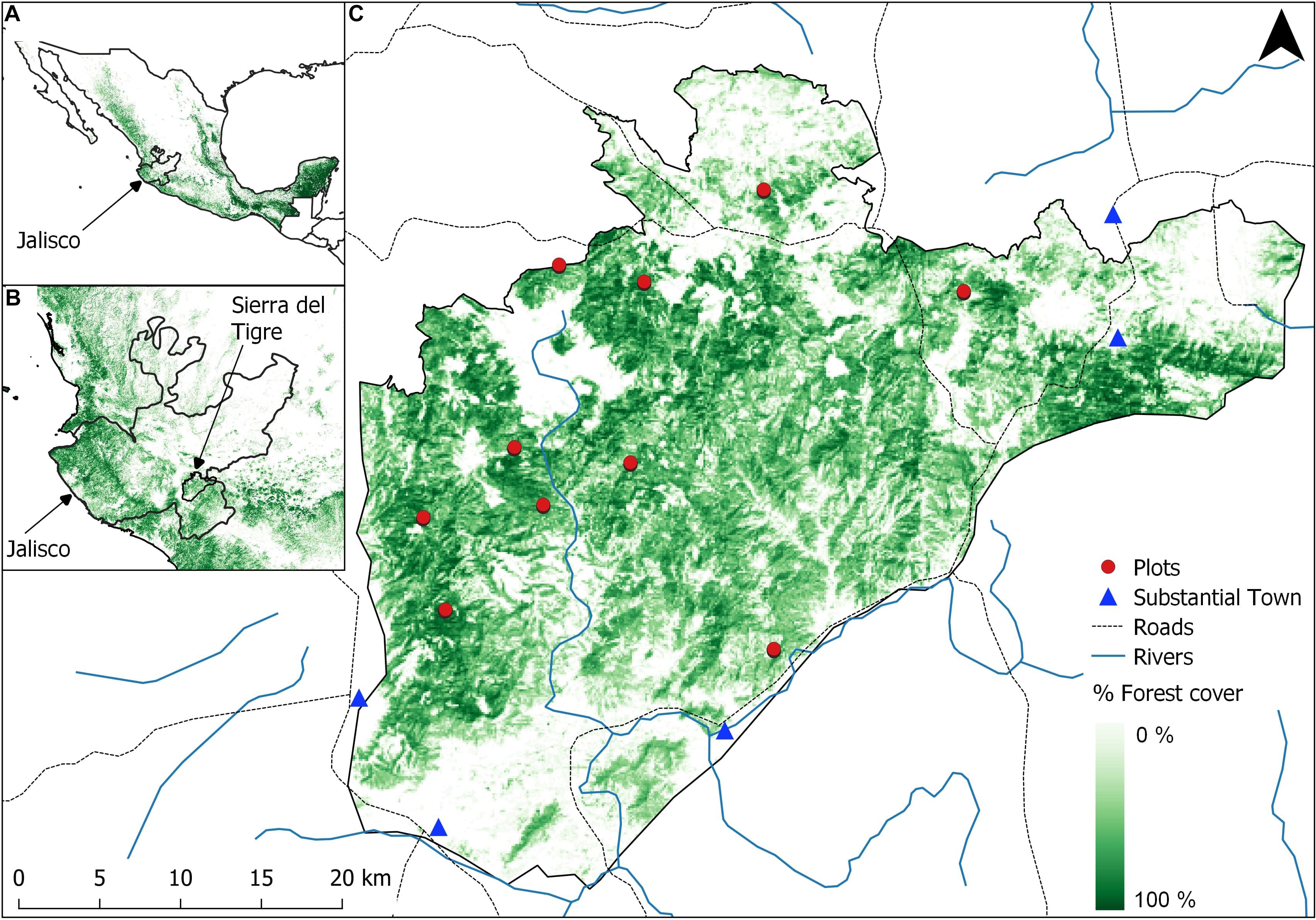
Figure 3. (A) Location of Jalisco state in Mexico (B). Location of the Sierra del Tigre study site within Jalisco, and (C). location of degradation plots (red points) within Sierra del Tigre.% forest cover for the year 2010 across Mexico taken from Hansen et al. (2013).

FIGURE 4

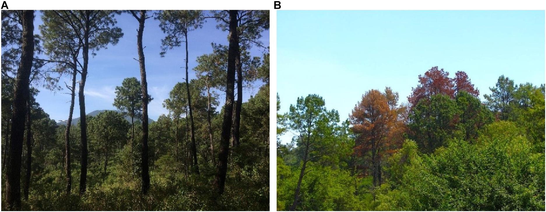
Figure 4. (A) Healthy Pine/Oak forest in Sierra del Tigre, Jalisco. (B) Dead pine trees (Pinus spp.) infected by Dendroctonus spp. in Sierra del Tigre.

In recent years, degradation has been linked to forest fires (Marín et al., 2018), which are common during the dry season in central Mexico and an outbreak of bark beetles (Dendroctonus spp.) that has caused widespread mortality of pines (Figure 4B). Sierra del Tigre is within a high risk zone for beetle outbreaks (Salinas-Moreno et al., 2010). Such outbreaks of beetles are particularly common in weakened forest stands following both natural and anthropogenic disturbances including; fire, drought, logging and land-use change (Salinas-Moreno et al., 2010), therefore the presence of these stress factors in Sierra del Tigre increases the likelihood of beetle outbreaks. Tree mortality in this zone is related to both death of infected trees and from management interventions, which involve cutting infected trees to prevent the spread of the disease, causing further widespread degradation.

Sample Design and Data Analysis

A trial network of ten plots (25 m × 200 m; 0.5 ha per plot) was established in Sierra del Tigre following the protocol described above, between September 2017 and December 2017 (Census 1). Plots were located at random within areas that were known to be experiencing degradation (equivalent to zone 1 stratification in Figure 1). These plots were measured again between October 2018 and December 2018 (Census 2), with a mean census interval of 1.04 years. All trees ≥10 cm DBH were measured, identified to species and given an X and Y coordinate used for relocation. Plot data was used to estimate AGB using the equation from Chave et al. (2014).

$$\text{AGB}=0.0673X{(\mathrm{\rho }DB{H}^{2}H)}^{0.976}(1)$$

where ρ = Wood density (g cm³), DBH = Diameter (cm), H = Height (m). For each individual the species-specific wood density (n = 6) was obtained from the global wood density database (Zanne et al., 2009), where species-specific wood density was unavailable, genus mean wood density (n = 22), or plot mean wood density (n = 6) was used. Whilst we recommend measuring the height of every individual in plots, we were unable to do this in the demonstration plot network, due to time constraints and the relatively high stem density. However, due to the type of degradation in Sierra del Tigre (mortality from fire and pests), we do not believe this is a problem, as we would not expect reductions in tree height from broken stem, as would be expected following other forms of degradation, such as selective logging. For each plot we measured the height of ten individuals in each of the following size classes; 10–20 cm DBH, 20–40 cm DBH, and >40 cm DBH (n = 290). To predict the height of every individual, we developed a local height: DBH allometric model by fitting different linear and non-linear regression models to measured height data. We selected the height: DBH allometric model with the lowest Akaike’s Information Criterion (AIC) and Root-mean-square error (RMSE). We found the best-fit model was (Figure 5);

$$H=1.191DBH/(1+0.028477DBH)(2)$$

$$(\mathrm{RMSE}=5.23,\mathrm{AIC}=1788,\mathrm{DF}=288)$$

FIGURE 5

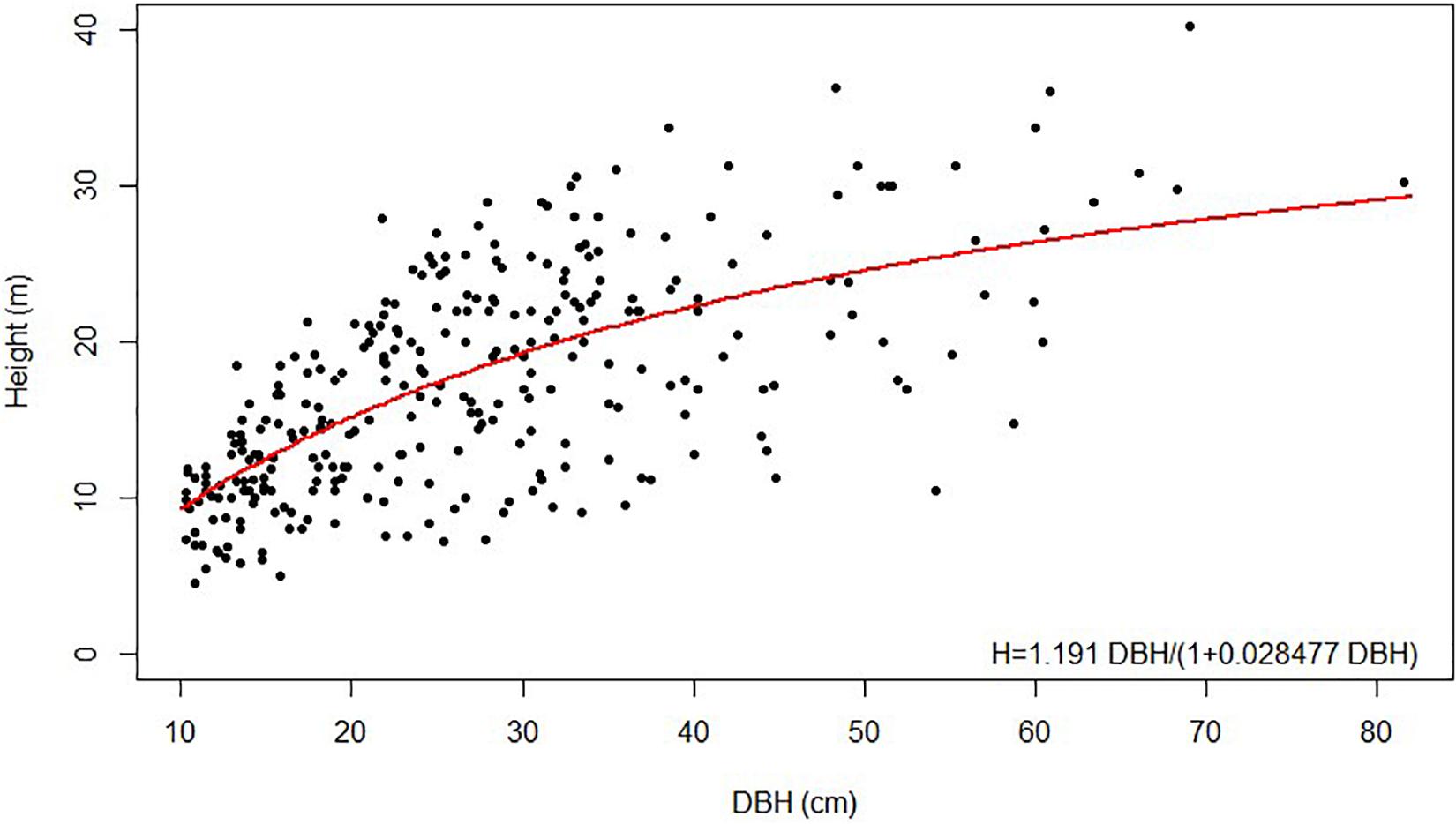
Figure 5. Height (m) and DBH (cm) of measured trees in Sierra del Tigre, showing best-fit model (red line).

When available, measured height was used to estimate AGB, otherwise Equation (2) was used to predict height.

Errors in plot level AGB estimates were propagated using the AGBmontecarlo() function in the BIOMASS package in R (Maxime et al., 2017), this accounts for tree level measurement errors in DBH, height and wood density, and errors in the allometric model used to estimate AGB. Error propagation gave a 95% confidence interval for plot level AGB estimated in Census 1 and Census 2, and for AGB change. Forest structural metrics including basal area (BA, m₂ ha^–1), mean DBH (cm), mean tree height (m), and stem density (stems ha^–1) were also calculated per plot. To understand forest dynamics we estimated above-ground woody productivity (AGWP) by summing the change in AGB between Census 1 and Census 2, plus the AGB of newly recruited stems in Census 2, and divided by the census interval (1) (Talbot et al., 2014). We also estimated tree mortality by summing AGB of stems alive in Census 1 that were dead by Census 2, and dividing by census interval (2) as below.

$$\text{AGWP}=\text{AGB}\mathrm{\Delta }+{\text{AGB}}_{new}/\text{CI}(3)$$

$$\text{Mortality}={\text{AGB}}_{dead}/\text{CI}(4)$$

where: AGBΔ = AGB Change (Mg ha^–1) between C1 and C2, AGB_new = AGB in new stems (Mg ha^–1) in C2, AGB_dead = AGB of live stems (Mg ha^–1) in C1 dead by C2, and CI = census interval (years).

Results

Data Collection and Relocation of Trees

As a proof of concept for this methodology, ten plots were established in Sierra del Tigre following the degradation PSP protocol. Using a combination of GPS coordinates and plot maps (Figure 6), which showed location of individuals, DBH, tree condition and other census data such as species, individual trees could be tracked across censuses without the need for permanent markers (Figures 7A,B). We were successfully able to relocate all plots with the exception of plot 6, which was clear-cut for Avocado production, and therefore access was prohibited. As this plot was clear-cut, we assumed a total loss of trees and AGB and classed it as ‘deforested’ for analysis. Figure 6 shows an example plot map for plot 8, plot maps showed a large number of trees damaged and in poor health due to fire in Census 1. By Census 2 many of these trees were dead and had been felled (Figures 7C,D). Plot data was collected by FIPRODEFO in Census 1 and Census 2. However, different field teams were used for each census, suggesting that individual trees could be identified using plot maps and previous census data, and that the same field technician is not needed to successfully relocate plots.

FIGURE 6

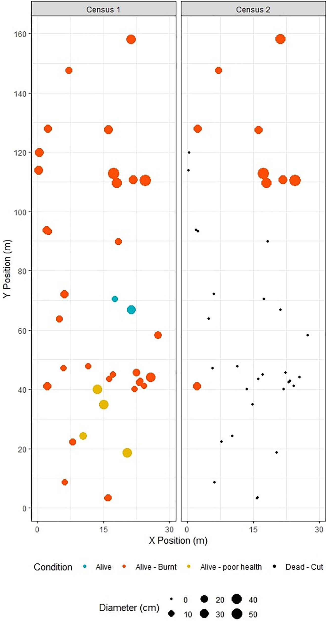
Figure 6. Example map of plot 8 in census 1 and census 2, showing live trees in census 1 and degradation in census 2. Maps show location of trees within plot, colours show condition of individual trees, size of point shows DBH (cm). Figure is not to scale.

FIGURE 7

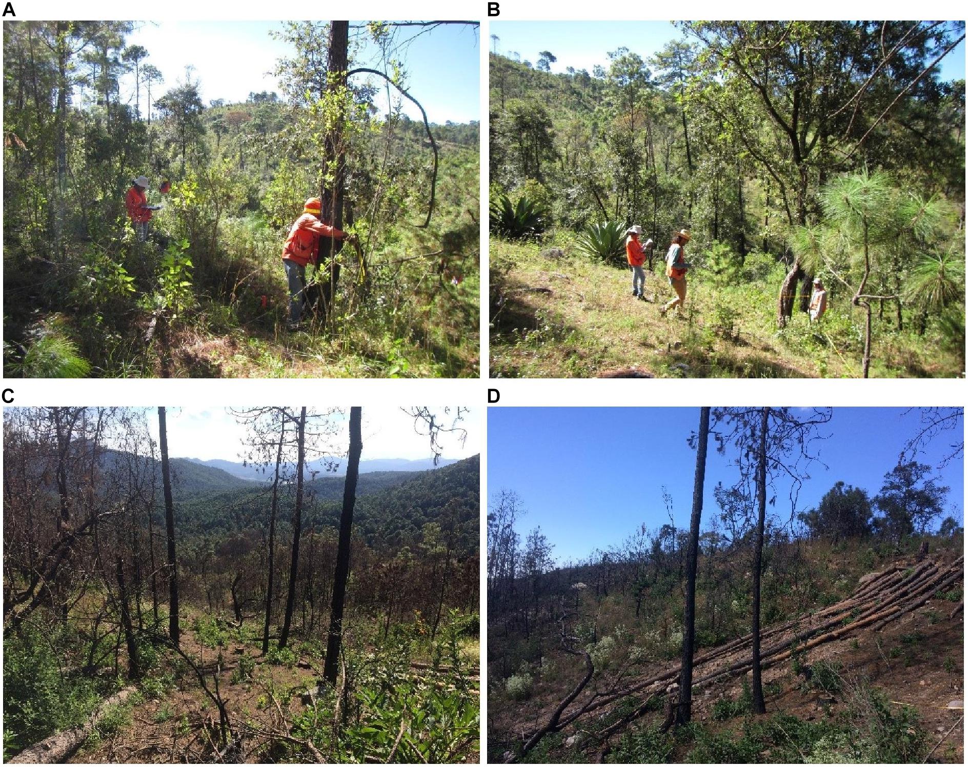
Figure 7. The FIPRODEFO field team (A) measuring forest plots following the degradation PSP protocol and (B) using plot maps to relocate individual trees. Plot 8 in census 2 showing (C) standing live stems damaged by fire and stumps and (D) trunks of cut stems.

Changes in Plot AGB and Structure

Live AGB in Census 1 ranged from 8.4 Mg ha^–1 to 140.8 Mg ha^–1, by Census 2 live AGB ranged from 0 Mg ha^–1 to 144.2 Mg ha^–1 (Table 2). Above-ground biomass reduced in four of the ten plots, notably the plot with the highest AGB in Census 1 (plot 6) was clear felled for avocado production, losing 140.8 Mg ha^–1 (Table 2). In the three remaining plots (plot 2, 8, and 9), AGB loss ranged from 3.7 to 16.5 Mg ha^–1 between Census 1 and 2, or a proportional AGB loss of between 4.2 and 42.7% (Table 2).

TABLE 2

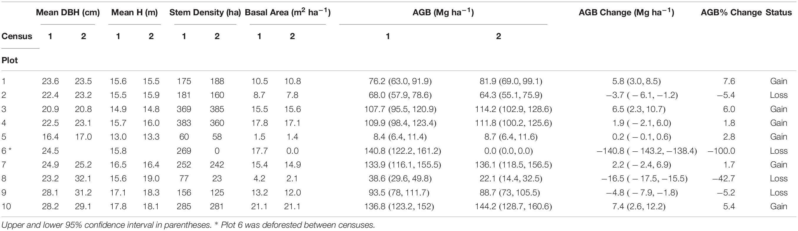
Table 2. Plot structural metrics in Census 1 (2017) and Census 2 (2018) in Live stems, AGB change and AGB% Change between Census 1 and Census 2, and plot status (Gain = AGB increase, Loss = AGB decrease).

The loss of AGB in plots 2, 8, and 9 was linked to a reduction in basal area by an average of 1.4 m² ha^–1 and a reduction in stem density by 35 stems ha^–1 between Census 1 and 2 (Table 2). Despite reductions in BA and stem density, mean DBH and height both increased between Census 1 and 2, suggesting reductions in stem density were related to smaller stems dying or being removed (Table 2). In six of the ten plots AGB increased by an average of 4.0 Mg ha^–1, or a 4.2% increase in AGB. Once the effects of mortality were accounted for, AGWP – i.e., the woody production of stems alive in both census plus newly recruited stems – was 4.5 Mg ha^–1 yr^–1 (± 1.9, 95% CI).

The forest of Sierra del Tigre had already experienced disturbance prior to plot establishment. In Census 1 there was an average of 57 (± 48) standing dead trees ha^–1, containing a mean AGB of 5.8 Mg ha^–1 (± 4.4), this assumes no decomposition of standing dead stems and therefore is likely to be a slight over-estimate of AGB. However, as these were standing rather than downed dead stems it is unlikely that they were very heavily decayed (these stems were not re-measured in Census 2). Based on tree codes used to assess mode of death, fire was by far the dominant cause of death with 84.3% of standing dead stems killed due to fire. An average of 18 stems ha^–1 died between Census 1 and Census 2, with a mortality of 4.5 Mg ha^–1 yr^–1 (±3.7, i.e., the mean AGB loss per ha from stems that died between Census 1 and Census 2).

In Census 1 the frequency distribution of stems exhibited an inverse J shape, typical of less disturbed forests (Figure 8). By Census 2 the plots which had gained AGB (i.e., had not been disturbed, n = 6) had some changes, with a reduction in small stems (10-20 cm) of 24%, however, the frequency distribution still exhibited an inverse J shape. By contrast, in plots that had lost AGB (i.e., degraded plots, excluding the deforested plot, n = 3), there was a big change in frequency distribution by Census 2, with the number of small stems (10-20cm) reducing by 75% and the number of stems in size classes 20-30 cm, 30-40 cm, and >40 cm reducing by 49%, 53%, and 28%, respectively (Figure 8). Meanwhile the deforested plot had lost all stems.

FIGURE 8

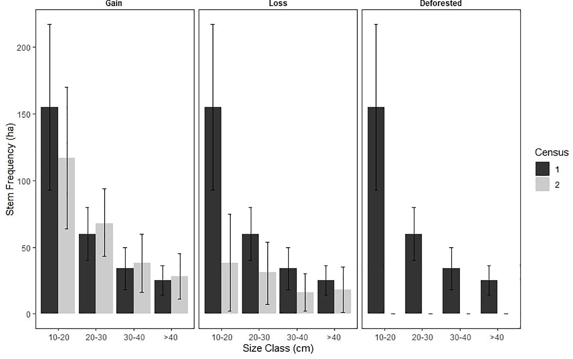
Figure 8. Frequency distribution of stems (ha^–1) in census 1 and 2 for plots that gained AGB (undisturbed plots), plots that lost AGB (degraded plots) and the deforested plot (Plot 6). Deforested plot (Plot 6) was separated from other AGB loss plots as it represented total deforestation rather than degradation. Error bars show 95% confidence intervals.

Discussion

We have presented a new protocol for forest plots, specifically designed for detecting forest degradation. We successfully trialled this protocol in forests undergoing degradation in Mexico. Using GPS coordinates and accurate plots maps (e.g., Figure 7), it was possible to relocate the plots and trees successfully despite the lack of tree tags. We detected both deforestation and forest degradation occurring in plots between censuses, as well as observing finer scale changes in forest structure and growth in the non-disturbed plots. Different field teams carried out Census 1 and Census 2, suggesting that the ability to remeasure plots was not due to field teams being familiar with the site, but rather that plot maps provided sufficient information for successful remeasurement. In more heavily degraded plots or following a longer census interval, relocating unmarked plots will be more challenging. However, our data suggest that an experienced field team should be able to relocate plots even following extreme degradation: plot 8 lost 70% of its stems between Census 1 and Census 2, and field teams were still able to successfully relocate individuals. Based on this case study, we believe our methodology could be applied more widely in other forest types with no or minimal adjustments.

The main benefit of this protocol is the speed of establishment, which was about half a day per plot with a team of 5–6 people (3 person days). This is much quicker than other PSP protocols, which require much more time for laying out of the plot, tagging and painting trees, such as the Rainfor protocol, which takes up to 11 person days to establish an equivalent sized 0.5 ha plot, nearly 4 time longer than the protocol described here (Phillips et al., 2009). As we found only three of the ten plots lost AGB, this reduction in the speed of establishment is important as it means more plots could be established in a shorter timeframe allowing a wider spatial distribution of ground data, and a broader spatial sampling. Using this new Forest Degradation PSP Protocol we were able to detect degradation events over a short time window within the demonstration plot network.

Degradation vs. Natural Changes

The data brought up an interesting question about what level of change constitutes degradation. All the plots in the demonstration network changed in biomass over the census period; however, it was clear that some small reductions in AGB and stem density did not constitute degradation. Many small patches of forest will naturally lose AGB in a given year due to tree mortality, therefore not all AGB losses between census periods are from anthropogenic disturbance. To determine if degradation has taken place it may be suitable to create a “cut-off” point for degradation based on the magnitude of negative changes in AGB or forest structure, where only losses greater than this cut-off point are classified as degradation. Determining what would be a suitable cut-off point needs to be based on local conditions rather than just selecting an arbitrary value for AGB loss and applying it across entire landscapes or region (Thompson et al., 2013). If all losses of AGB are assumed to be degradation then natural forest changes would also be included whereas, if a very high AGB loss is required for land to be classified as degraded, then this may exclude more small scale degrading practices such as fuelwood extraction (Vásquez-Grandón et al., 2018). Furthermore, the difference between absolute AGB change and percentage AGB change must be considered. For example, if a forest stand of 50 Mg ha^–1 lost 10 Mg ha^–1, this equates to a 20% loss of AGB, this is proportionally much greater than a forest of 150 Mg ha^–1 that loses 10 mg ha^–1, which would equate to a 7% loss of AGB. Therefore considering the percentage AGB loss alongside absolute AGB loss may help determine whether a forest is degraded.

Another means of determining whether degradation occurred is by attributing changes within plots to particular degrading activities. For example, if a cut tree stump is found within a plot then we can be certain that this individual loss constitutes anthropogenic degradation, regardless of a percentage change in AGB. However, detecting such changes is dependent on the census interval. Shorter census intervals increase the likelihood of locating stumps of cut individuals as decomposition of coarse woody debris can be rapid, with residency times of <4 years in tropical forests (Gora et al., 2019). Conversely, longer census intervals mean that identifying the specific cause of tree mortality is more challenging as there is more unobserved growth (Talbot et al., 2014). Using the method presented in this paper, we were able to attribute mortality of 83% of individuals to fire, showing that this protocol can determine not only changes in AGB but also the cause of degradation. Attributing changes within plots to people becomes opaque with some forms of degradation such as fire. With tree cutting it is clear that anthropogenic disturbance has taken place, whereas with fire it is not always clear if fires are natural or were started by people. Whilst forest degradation often refers to anthropogenic disturbances, natural degradation events such as wildfire must also be considered. Pearson et al. (2017) estimated that 17% of tropical forest degradation emissions come from fires and therefore they are an important source of emissions to quantify. However, identifying the difference between wildfires and human-ignited fires may be important as different policy and management interventions are required to prevent them. Whilst natural wildfires could be managed through the additions of firebreaks, reducing human-ignited fires – for example from escaped agricultural burning or attempted land-use change - requires cooperative forest management policies between people living near forest areas and forest managers (Chas-Amil et al., 2015).

Suitability of Protocol

Forest plots of similar dimensions have previously been used in degraded forest sites and in remote sensing analysis to map AGB, suggesting that the plot design used in this protocol is suitable for monitoring forest degradation. In the Congo basin plots of 25 m × 200 m were used to assess floristic composition in logged over forest (Réjou-Méchain et al., 2011; Ouédraogo et al., 2016). Plots of 20 m × 200 m have also been used in Cameroon, to calibrate SAR data to map forest AGB (Mitchard et al., 2011).

One novel aspect of this protocol making it particularly suited to forest degradation monitoring is the selective sample design, which ensures that PSPs are located within areas at higher risk of degradation or areas that are undergoing degradation. This is areas such as, close to roads, forest edges and settlements where there is a higher population density (Bryan et al., 2013; Kleinschroth et al., 2019), or within logging areas. By locating plots in areas that have a higher likelihood of being degraded, a lower sampling density can capture degradation. Biasing plot locations toward areas that are undergoing degradation is important for two reasons. Firstly, to accurately capture AGB losses and structural changes related to degradation on the ground. Secondly, by focusing on degraded areas it ensures there are sufficient ground truthing points for accurate calibration and validation of remote sensing products used to monitor degradation at larger spatial scales.

The degradation PSP protocol presented here is an improvement on existing protocols for monitoring degradation, as it allows for accurate estimate of AGB changes that result from degradation within every plot, Furthermore, such data can be used for calibration and validation of remote sensing products. Typically forest degradation protocols use single census inventory data, to compare degraded forest with intact reference forest, taking the mean AGB (Mg ha^–1) in intact and degraded forests and assume that the difference in AGB is equivalent to the average AGB loss from degradation (e.g., Maniatis and Mollicone, 2010). However, this approach has some shortcomings; firstly, it is based on the false assumption that all forest (of a given forest type in a region) has the same starting AGB prior to degradation, and does not account for spatial heterogeneity in forest AGB. Secondly, by using single census data, you cannot detect the ongoing or gradual losses of AGB that are indicative of degradation. Finally, a single census approach is less useful for calibration and validation in remote sensing analysis to map degradation, as change data from plots, necessary for ground truthing, are not available.

The converse of our sampling approach is fully randomised designs. However, due to the heterogeneous and non-random distribution of degradation, such sample designs are likely inappropriate for monitoring degradation. Particularly in areas with low levels of degradation as the probability of encountering degraded areas is low, so unless resources are quasi-unlimited it is unlikely to be a sensible approach. Such randomised designs are often adopted for national forest inventory (NFI) plot networks, such as the Mexican or Zambian NFI (CONAFOR, 2015; Zambia, 2016). Countries are now required to report emissions from forest degradation to the UNFCCC under their commitments to the Paris Agreement (UNFCCC, 2015), principally under the reducing emissions from deforestation and forest degradation (REDD+) mechanism (Pistorius, 2012). Current guidelines suggest existing NFI networks can be used for monitoring forest degradation (IPCC, 2019), therefore many countries use such NFI networks for reporting. However, this approach will inevitably lead to high uncertainty in degradation estimates, as the untargeted nature of plots means that few will be degraded.

Errors in estimates of degradation are problematic for two reasons. Firstly, we need to improve global estimates of emissions from forest degradation; if we do not have accurate estimates of emissions then we are unable to appropriately reduce and mitigate those emissions. Secondly, there are financial mechanisms in place to support countries efforts to monitor forest degradation such as the World Bank’s Carbon Fund (Forest Carbon Partnership Facility, 2016), therefore if countries are underreporting forest degradation they could be rendering themselves ineligible for funding which could help tackle the problem.

We hope this new protocol is part of a solution to this problem, and encourage its adoption. We recognise that in some locations and ecological/disturbance systems (e.g., degraded mangrove forests) it will need to be modified or will not be appropriate, but hopefully some of the design features and considerations covered here will help improve monitoring of forest degradation.

Data Availability Statement

The datasets presented in this article are not readily available because the data were collected jointly between University of Edinburgh and FIPRODEFO – Trust for the Administration of the Forest Development Program of the State of Jalisco. Requests for data must be made to the corresponding author and co-author HN. Requests to access the datasets should be directed to CW, c.wheeler@ed.ac.uk and HN, tecnico.geomatica@fiprodefo.gob.mx.

Author Contributions

CW and EM conceived the ideas and designed the methodology. CW, HN, GI, and JM collected the data. CW analysed the data and led the writing of the manuscript. All authors contributed critically to the drafts and gave final approval for publication.

Funding

This study was funded by the UK Space Agency’s International partnership Programme under the Forests 2020 project (https://ecometrica.com/space/forests2020), managed by Ecometrica.

Conflict of Interest

The authors declare that the research was conducted in the absence of any commercial or financial relationships that could be construed as a potential conflict of interest.

Publisher’s Note

All claims expressed in this article are solely those of the authors and do not necessarily represent those of their affiliated organizations, or those of the publisher, the editors and the reviewers. Any product that may be evaluated in this article, or claim that may be made by its manufacturer, is not guaranteed or endorsed by the publisher.

Acknowledgments

We would like to thank the field assistance at FIPRODEFO (Trust for the Administration of the Forest Development Program of the State of Jalisco) who helped with plot data collection.

Supplementary Material

The Supplementary Material for this article can be found online at: https://www.frontiersin.org/articles/10.3389/ffgc.2021.655280/full#supplementary-material

References

Baccini, A., Walker, W., Carvalho, L., Farina, M., Sulla-Menashe, D., and Houghton, R. A. (2017). Tropical forests are a net carbon source based on aboveground measurements of gain and loss. Science 358, 230–234. doi: 10.1126/science.aam5962

PubMed Abstract | CrossRef Full Text | Google Scholar

Brienen, R. J., Phillips, O., Feldpausch, T., Gloor, E., Baker, T., Lloyd, J., et al. (2015). Long-term decline of the Amazon carbon sink. Nature 519, 344–348.

Google Scholar

Brinck, K., Fischer, R., Groeneveld, J., Lehmann, S., De Paula, M. D., Pütz, S., et al. (2017). High resolution analysis of tropical forest fragmentation and its impact on the global carbon cycle. Nat. Commun. 8:14855.

Google Scholar

Bryan, J. E., Shearman, P. L., Asner, G. P., Knapp, D. E., Aoro, G., and Lokes, B. (2013). Extreme differences in forest degradation in Borneo: comparing practices in Sarawak, Sabah, and Brunei. PLoS One 8:e69679. doi: 10.1371/journal.pone.0069679

PubMed Abstract | CrossRef Full Text | Google Scholar

Bullock, E. L., Woodcock, C. E., Souza, C. Jr., and Olofsson, P. (2020). Satellite-based estimates reveal widespread forest degradation in the Amazon. Glob. Change Biol. 26, 2956–2969. doi: 10.1111/gcb.15029

PubMed Abstract | CrossRef Full Text | Google Scholar

Bustamante, M. M. C., Roitman, I., Aide, T. M., Alencar, A., Anderson, L. O., Aragão, L., et al. (2016). Toward an integrated monitoring framework to assess the effects of tropical forest degradation and recovery on carbon stocks and biodiversity. Glob. Change Biol. 22, 92–109. doi: 10.1111/gcb.13087

PubMed Abstract | CrossRef Full Text | Google Scholar

Campbell, G., Kuehl, H., Diarrassouba, A., N’goran, P. K., and Boesch, C. (2011). Long-term research sites as refugia for threatened and over-harvested species. Biol. Lett. 7, 723–726. doi: 10.1098/rsbl.2011.0155

PubMed Abstract | CrossRef Full Text | Google Scholar

Chaplin-Kramer, R., Ramler, I., Sharp, R., Haddad, N. M., Gerber, J. S., West, P. C., et al. (2015). Degradation in carbon stocks near tropical forest edges. Nat. Commun. 6:10158.

Google Scholar

Chas-Amil, M. L., Prestemon, J. P., Mcclean, C. J., and Touza, J. (2015). Human-ignited wildfire patterns and responses to policy shifts. Appl. Geogr. 56, 164–176. doi: 10.1016/j.apgeog.2014.11.025

CrossRef Full Text | Google Scholar

Chave, J., Davies, S. J., Phillips, O. L., Lewis, S. L., Sist, P., Schepaschenko, D., et al. (2019). Ground data are essential for biomass remote sensing missions. Surv. Geophys. 40, 863–880. doi: 10.1007/s10712-019-09528-w

CrossRef Full Text | Google Scholar

Chave, J., Réjou-Méchain, M., Búrquez, A., Chidumayo, E., Colgan, M. S., Delitti, W. B. C., et al. (2014). Improved allometric models to estimate the aboveground biomass of tropical trees. Glob. Change Biol. 20, 3177–3190.

Google Scholar

CONAFOR (2015). National Forest Reference Emission Level Proposal México. Mexico: National Forestry Commission.

Google Scholar

Condit, R. (1998). Tropical Forest Census Plots: Methods and Results from Barro Colorado Island, Panama and a Comparison with other Plots. Berlin: Springer Science & Business Media.

Google Scholar

De Andrade, R. B., Balch, J. K., Parsons, A. L., Armenteras, D., Roman-Cuesta, R. M., and Bulkan, J. (2017). Scenarios in tropical forest degradation: carbon stock trajectories for REDD+. Carbon Balance Manag. 12:6.

Google Scholar

Esquivel-Muelbert, A., Baker, T. R., Dexter, K. G., Lewis, S. L., Brienen, R. J. W., Feldpausch, T. R., et al. (2019). Compositional response of Amazon forests to climate change. Glob. Change Biol. 25, 39–56.

Google Scholar

FAO (2010). Global Forest Resources Assessment 2010. FAO Forestry paper 163. Rome: Food and Agricultural Organization of the UN.

Google Scholar

FAO (2015). Global Forest Resources Assessment 2015. Rome: Food and Agricultural Organization of the UN.

Google Scholar

FAO (2020). Integration of Remote-Sensing and Ground-Based Observations for Estimation of Emissions and Removals of Greenhouse Gases In Forests: Methods and Guidance From The Global Forest Observations Initiative. Rome: FAO.

Google Scholar

Fauset, S., Baker, T. R., Lewis, S. L., Feldpausch, T. R., Affum-Baffoe, K., Foli, E. G., et al. (2012). Drought-induced shifts in the floristic and functional composition of tropical forests in Ghana. Ecol. Lett. 15, 1120–1129. doi: 10.1111/j.1461-0248.2012.01834.x

PubMed Abstract | CrossRef Full Text | Google Scholar

Fayolle, A., Engelbrecht, B., Freycon, V., Mortier, F., Swaine, M., Réjou-Méchain, M., et al. (2012). Geological substrates shape tree species and trait distributions in African moist forests. PLoS One 7:e42381. doi: 10.1371/journal.pone.0042381

PubMed Abstract | CrossRef Full Text | Google Scholar

Forest Carbon Partnership Facility (2016). Carbon Fund Methodological Framework. USA: Forest Carbon Partnership Facility.

Google Scholar

Ghazoul, J., Burivalova, Z., Garcia-Ulloa, J., and King, L. A. (2015). Conceptualizing forest degradation. Trends Ecol. Evol. 30, 622–632. doi: 10.1016/j.tree.2015.08.001

PubMed Abstract | CrossRef Full Text | Google Scholar

Global Forest Watch (2014). World Recources Institute. Available online at: http//www.globalforestwatch.org/ (accessed April 07, 2020).

Google Scholar

Gora, E. M., Kneale, R. C., Larjavaara, M., and Muller-Landau, H. C. (2019). Dead wood necromass in a moist tropical forest: stocks, fluxes, and spatiotemporal variability. Ecosystems 22, 1189–1205. doi: 10.1007/s10021-019-00341-5

CrossRef Full Text | Google Scholar

Hansen, M. C., Potapov, P. V., Moore, R., Hancher, M., Turubanova, S. A., Tyukavina, A., et al. (2013). High-resolution global maps of 21st-century forest cover change. Science 342, 850–853. doi: 10.1126/science.1244693

PubMed Abstract | CrossRef Full Text | Google Scholar

Herold, M., Román-Cuesta, R. M., Mollicone, D., Hirata, Y., Van Laake, P., Asner, G. P., et al. (2011). Options for monitoring and estimating historical carbon emissions from forest degradation in the context of REDD+. Carbon Balance Manag. 6:13.

Google Scholar

IPCC (2019). 2019 Refinement to the 2006 IPCC Guidelines for National Greenhouse Gas Inventories, eds E. Calvo Buendia, K. Tanabe, A. Kranjc, J. Baasansuren, M. Fukuda, S. Ngarize, et al. (Switzerland: Intergovernmental Panel on Climate Change).

Google Scholar

Kleinschroth, F., Laporte, N., Laurance, W. F., Goetz, S. J., and Ghazoul, J. (2019). Road expansion and persistence in forests of the Congo Basin. Nat. Sustain. 2, 628–634. doi: 10.1038/s41893-019-0310-6

CrossRef Full Text | Google Scholar

Lewis, S. L., Edwards, D. P., and Galbraith, D. (2015). Increasing human dominance of tropical forests. Science 349, 827–832. doi: 10.1126/science.aaa9932

PubMed Abstract | CrossRef Full Text | Google Scholar

Lewis, S. L., Lopez-Gonzalez, G., Sonke, B., Affum-Baffoe, K., Baker, T. R., Ojo, L. O., et al. (2009). Increasing carbon storage in intact African tropical forests. Nature 457, 1003–1006.

Google Scholar

Lewis, S. L., Sonké, B., Sunderland, T., Begne, S. K., Lopez-Gonzalez, G., Van Der Heijden, G. M. F., et al. (2013). Above-ground biomass and structure of 260 African tropical forests. Philos. Trans. R Soc. B Biol. Sci. 368:20120295.

Google Scholar

Lopez-Gonzalez, G., Lewis, S. L., Burkitt, M., and Phillips, O. L. (2011). ForestPlots.net: a web application and research tool to manage and analyse tropical forest plot data. J. Veg. Sci. 22, 610–613. doi: 10.1111/j.1654-1103.2011.01312.x

CrossRef Full Text | Google Scholar

Maniatis, D., and Mollicone, D. (2010). Options for sampling and stratification for national forest inventories to implement REDD+ under the UNFCCC. Carbon Balance Manag. 5:9.

Google Scholar

Marín, P.-G., Julio, C. J., Dante Arturo, R.-T., and Daniel Jose, V.-N. (2018). Drought and spatiotemporal variability of forest fires across Mexico. Chin. Geogr. Sci. 28, 25–37. doi: 10.1007/s11769-017-0928-0

CrossRef Full Text | Google Scholar

Matangaran, J. R., Putra, E. I., Diatin, I., Mujahid, M., and Adlan, Q. (2019). Residual stand damage from selective logging of tropical forests: a comparative case study in central Kalimantan and West Sumatra, Indonesia. Glob. Ecol. Conserv. 19:e00688. doi: 10.1016/j.gecco.2019.e00688

CrossRef Full Text | Google Scholar

Maxime, R. M., Ariane, T., Camille, P., Jérôme, C., and Bruno, H. (2017). Biomass: an r package for estimating above-ground biomass and its uncertainty in tropical forests. Methods Ecol. Evol. 8, 1163–1167. doi: 10.1111/2041-210x.12753

CrossRef Full Text | Google Scholar

McNicol, I. M., Ryan, C. M., and Mitchard, E. T. A. (2018). Carbon losses from deforestation and widespread degradation offset by extensive growth in African woodlands. Nat. Commun. 9:3045.

Google Scholar

Michalcová, D., Lvončík, S., Chytrý, M., and Hájek, O. (2011). Bias in vegetation databases? A comparison of stratified-random and preferential sampling. J. Veget. Sci. 22, 281–291. doi: 10.1111/j.1654-1103.2010.01249.x

CrossRef Full Text | Google Scholar

Mitchard, E. T. A. (2018). The tropical forest carbon cycle and climate change. Nature 559, 527–534. doi: 10.1038/s41586-018-0300-2

PubMed Abstract | CrossRef Full Text | Google Scholar

Mitchard, E. T., Saatchi, S. S., Lewis, S., Feldpausch, T., Woodhouse, I. H., Sonké, B., et al. (2011). Measuring biomass changes due to woody encroachment and deforestation/degradation in a forest–savanna boundary region of central Africa using multi-temporal L-band radar backscatter. Remote Sens. Environ. 115, 2861–2873. doi: 10.1016/j.rse.2010.02.022

CrossRef Full Text | Google Scholar

Mitchell, A. L., Rosenqvist, A., and Mora, B. (2017). Current remote sensing approaches to monitoring forest degradation in support of countries measurement, reporting and verification (MRV) systems for REDD. Carbon Balance Manag. 12:9.

Google Scholar

Noruzi, M., and Vargas, J. (2009). Atenquique’s environmental and economic development shrinkage in Globalization era. Bus. Intell. J. 2, 343–354.

Google Scholar

Ouédraogo, D.-Y., Fayolle, A., Gourlet-Fleury, S., Mortier, F., Freycon, V., Fauvet, N., et al. (2016). The determinants of tropical forest deciduousness: disentangling the effects of rainfall and geology in central Africa. J. Ecol. 104, 924–935. doi: 10.1111/1365-2745.12589

CrossRef Full Text | Google Scholar

Pearson, T. R. H., Brown, S., Murray, L., and Sidman, G. (2017). Greenhouse gas emissions from tropical forest degradation: an underestimated source. Carbon Balance Manag. 12:3.

Google Scholar

Peña-Claros, M., Fredericksen, T. S., Alarcón, A., Blate, G. M., Choque, U., Leaño, C., et al. (2008). Beyond reduced-impact logging: Silvicultural treatments to increase growth rates of tropical trees. For. Ecol. Manag. 256, 1458–1467. doi: 10.1016/j.foreco.2007.11.013

CrossRef Full Text | Google Scholar

Phillips, O., Baker, T., Feldpausch, T., and Brienen, R. (2009). RAINFOR Field Manual for Plot Establishment and Remeasurement. Available online at: http://www.rainfor.org/en/manuals (accessed January 8, 2021).

Google Scholar

Pinheiro, T. F., Escada, M. I. S., Valeriano, D. M., Hostert, P., Gollnow, F., and Müller, H. (2016). Forest degradation associated with logging frontier expansion in the amazon: the br-163 region in southwestern Pará, Brazil. Earth Interact. 20, 1–26. doi: 10.1175/ei-d-15-0016.1

CrossRef Full Text | Google Scholar

Pistorius, T. (2012). From RED to REDD+: the evolution of a forest-based mitigation approach for developing countries. Curr. Opin. Environ. Sustain. 4, 638–645. doi: 10.1016/j.cosust.2012.07.002

CrossRef Full Text | Google Scholar

Pote, J., Shackleton, C., Cocks, M., and Lubke, R. (2006). Fuelwood harvesting and selection in Valley Thicket, South Africa. J. Arid Environ. 67, 270–287. doi: 10.1016/j.jaridenv.2006.02.011

CrossRef Full Text | Google Scholar

Read, L., and Lawrence, D. (2003). Recovery of biomass following shifting cultivation in dry tropical forests of the Yucatan. Ecol. Appl. 13, 85–97. doi: 10.1890/1051-0761(2003)013[0085:robfsc]2.0.co;2

CrossRef Full Text | Google Scholar

Réjou-Méchain, M., Fayolle, A., Nasi, R., Gourlet-Fleury, S., Doucet, J.-L., Gally, M., et al. (2011). Detecting large-scale diversity patterns in tropical trees: can we trust commercial forest inventories? For. Ecol. Manag. 261, 187–194. doi: 10.1016/j.foreco.2010.10.003

CrossRef Full Text | Google Scholar

Ribeiro, G. H. P. M., Chambers, J. Q., Peterson, C. J., Trumbore, S. E., Magnabosco Marra, D., Wirth, C., et al. (2016). Mechanical vulnerability and resistance to snapping and uprooting for Central Amazon tree species. For. Ecol. Manag. 380, 1–10. doi: 10.1016/j.foreco.2016.08.039

CrossRef Full Text | Google Scholar

Romero-Duque, L. P., Jaramillo, V. J., and Perez-Jimenez, A. (2007). Structure and diversity of secondary tropical dry forests in Mexico, differing in their prior land-use history. For. Ecol. Manag. 253, 38–47. doi: 10.1016/j.foreco.2007.07.002

CrossRef Full Text | Google Scholar

Salinas-Moreno, Y., Ager, A., Vargas, C. F., Hayes, J. L., and Zúñiga, G. (2010). Determining the vulnerability of Mexican pine forests to bark beetles of the genus Dendroctonus Erichson (Coleoptera: Curculionidae: Scolytinae). For. Ecol. Manag. 260, 52–61. doi: 10.1016/j.foreco.2010.03.029

CrossRef Full Text | Google Scholar

Sasaki, N., and Putz, F. E. (2009). Critical need for new definitions of “forest” and “forest degradation” in global climate change agreements. Conserv. Lett. 2, 226–232. doi: 10.1111/j.1755-263x.2009.00067.x

CrossRef Full Text | Google Scholar

Simula, M. (2009). Towards Defining Forest Degradation: Comparative Analysis of Existing Definitions. Rome: FAO.

Google Scholar

Speak, A., Escobedo, F. J., Russo, A., and Zerbe, S. (2018). Comparing convenience and probability sampling for urban ecology applications. J. Appl. Ecol. 55, 2332–2342. doi: 10.1111/1365-2664.13167

CrossRef Full Text | Google Scholar

Sullivan, M. J., Talbot, J., Lewis, S. L., Phillips, O. L., Qie, L., Begne, S. K., et al. (2017). Diversity and carbon storage across the tropical forest biome. Sci. Rep. 7, 1–12.

Google Scholar

Talbot, J., Lewis, S. L., Lopez-Gonzalez, G., Brienen, R. J. W., Monteagudo, A., Baker, T. R., et al. (2014). Methods to estimate aboveground wood productivity from long-term forest inventory plots. For. Ecol. Manag. 320, 30–38. doi: 10.1016/j.foreco.2014.02.021

CrossRef Full Text | Google Scholar

Thompson, I. D., Guariguata, M. R., Okabe, K., Bahamondez, C., Nasi, R., Heymell, V., et al. (2013). An operational framework for defining and monitoring forest degradation. Ecol. Soc. 18:20.

Google Scholar

UNFCCC (2009). Methodological guidance for activities relating to reducing emissions from deforestation and forest degradation and the role of conservation, sustainable management of forests and enhancement of forest carbon stocks in developing countries. Decision COP 15/4. New York, NY: United Nations Framework Convention on Climate Change.

Google Scholar

UNFCCC (2015). “The Paris agreement,” in Proceedings of the Conference of the Parties 21 (Paris: United Nations Framework Convention on Climate Change).

Google Scholar

USDA (2012). Mexico Avocado Annual Production and Exports Forcast. Washington, WA: USDA.

Google Scholar

USDA (2019). Mexico Avocado Annual Production and Exports Forcast. Washington, WA: USDA.

Google Scholar

Vásquez-Grandón, A., Donoso, P. J., and Gerding, V. (2018). Forest Degradation: When Is a Forest Degraded? Forests 9:726. doi: 10.3390/f9110726

CrossRef Full Text | Google Scholar

Zambia, R. O. (2016). Zambia’s Forest Reference Emissions Level Submission to the UNFCCC. Paris: United Nations Framework Convention on Climate Change.

Google Scholar

Zanne, A. E., Lopez-Gonzalez, G., Coomes, D. A., Ilic, J., Jansen, S., Lewis, S. L., et al. (2009). Global Wood Density Database. Available online at: http://hdl.handle.net/10255/dryad.235 (accessed January 8, 2021).

Google Scholar