Hierarchical Bayesian Small Area Estimation Using Weakly Informative Priors in Ecologically Homogeneous Areas of the Interior Western Forests

1. Introduction

The USDA Forest Service Forest Inventory and Analysis Program (FIA) collects a sample of inventory data nationwide to monitor status and trends in forested ecosystems at scales relevant for strategic-level planning. Increasingly, this network of valuable inventory plots is being called upon to answer questions relevant to forest land management which is below the spatial and temporal scales for which the sample was originally designed. Information is needed on resources lost and recovery rates within disturbance boundaries, on significant change in carbon sources and sinks, as well as on the state of the forests within individual counties, districts, or other small management units. There is strong interest in exploring methods to integrate extant inventory data with remotely sensed data through models that expand the capacity to estimate forest attributes over smaller domains in space and time.

A standard estimator that combines inventory data with remotely sensed data is the generalized regression estimator (Cassel et al., 1976) in which the inventory data are modeled and predicted over the domain of interest and then the observed data and predictions are aggregated to construct an estimator. Post-stratification (PS), a common estimation technique for national forest inventories (NFI) such as FIA, is a special case of the generalized regression estimator that incorporates a single, categorical auxiliary variable into the estimator (Särndal et al., 1992). Since the generalized regression estimator only makes use of data within the domain of interest, it is called a direct estimator. And, although leveraging auxiliary data typically improves the precision of a direct estimator, it tends to still not achieve adequate levels of precision when the sample size of the inventory data in the domain is small (Rao and Molina, 2015). Therefore, we consider here indirect estimators with their defining characteristic of borrowing strength from data outside the domain of interest. These domains are often classified as small areas and we will use the terms domain and small area interchangeably. When the indirect estimator explicitly relies on a model to link the data in the desired small area with data in other related small areas it is called a small area estimator. These linking models can be built either at the area level or unit (i.e., plot) level, depending on data availability and the strength of the relationships between the inventory data and remote sensing data at these two resolutions. We study area level models here because the inventory and remotely-sensed data we consider have strong linear trends at the area level and violate normality assumptions at the unit level. These estimators are constructed under either a frequentist framework where the quantities of interest are fixed, unknown values or a Bayesian framework where they are considered random variables. Key advantages of the Bayesian approach are that it allows the modeler to directly consider uncertainty between the small areas and to obtain distributions, not just point estimates and standard error estimates, for the parameters of interest.

A frequently utilized, and frequentist-based, indirect estimator is the empirical best linear unbiased prediction (EBLUP) estimator, which uses a linking model with random area-specific effects to borrow strength from related areas (Rao and Molina, 2015). The suitability of area and unit level EBLUP estimators to the small area applications found in NFIs have been studied extensively (Goerndt et al., 2011; Breidenbach and Astrup, 2012; Magnussen et al., 2017; Mauro et al., 2017; Coulston et al., 2021). This paper considers the Bayesian analog to the EBLUP, a hierarchical Bayesian (HB) estimator. These HB estimators are not commonly used in forest inventory research; however, they have been applied in a variety of other application areas ranging from poverty mapping to agriculture to transportation to employment (You et al., 2003; Vaish et al., 2010; Wang et al., 2012; Molina et al., 2014) to name a few. Within the NFI literature, Ver Planck et al. (2018) explored an area level HB estimator for estimating forest attributes and did find improvements in precision over the Horvitz-Thompson (HT) direct estimator.

In this paper, we explore the performance of the PS, the area level EBLUP, and the area level HB estimators at estimating the mean value of four response variables: basal area (m² per hectare), count of trees per hectare, above-ground biomass (kg per hectare), and net volume of trees (m³ per hectare), excluding rotten or form defects, across the Interior West (IW) of the US. We generate estimates within the subregion (ecosubsection) of a hierarchical system of ecological divisions. For both the EBLUP and HB approaches, we consider the impact of borrowing strength from two resolutions from upper hierarchical levels: ecosection and ecoprovince, at scales of thousands of acres and millions of acres, respectively. Leveraging the flexibility of the HB, we study the impacts of varying how prior information on the homogeneity of the modeled small areas is incorporated into the estimator. We find that when borrowing strength to the ecosection level and including weakly informative prior information about small area homogeneity with the area level HB estimator we can reduce variance substantially compared to other common estimators. Explorations of potential bias through comparison with the post-stratified estimator display almost no introduction of bias with this estimator. However, since we do not know the true mean of the response variable of interest, caution is warranted when making strong conclusions about bias.

2. Methods

2.1. Region of Study and FIA Data

This manuscript focuses on estimating the mean of several key forest attributes for the ecosubsections in the IW region of the United States (Figure 1), which encompasses the states of Arizona, Colorado, Idaho, Montana, Nevada, New Mexico, Utah, and Wyoming. The inventory data were collected by FIA using a geographically-based systematic sampling design, where each plot represents about 2,500 ha of land (Bechtold and Patterson, 2005) and cover a 10 year measurement cycle from 2007 to 2017. This sample of 86,065 inventory plots were downloaded on February 6, 2019 from the FIA database, version FIADB_1.8.9.99 (last updated Dec 3, 2018). Our analyses include the use of four variables from the FIA database as response variables: basal area (m² per hectare), count of trees per hectare, above-ground biomass (kg per hectare), and net volume (m³ per hectare). For remotely-sensed auxiliary variables, we consider a forest/non-forest classification used for post-stratifying in the IW (Blackard et al., 2008) and the 2016 National Land Cover Database percent tree canopy cover map (Yang et al., 2018), which has a spatial resolution of 30 m. Although each FIA plot consists of 4 subplots, response variables represent the aggregation of information at the plot level, and just the FIA plot center was intersected with the two auxiliary data layers. As input to the area-level estimators described below, both the percent canopy cover and proportions of forest and non-forest classes are averaged to the small area level for the IW. FIA data retrievals and processing of auxiliary data were done through the R package FIESTA (Frescino et al., 2015).

FIGURE 1

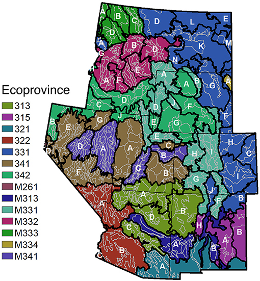
Figure 1. To illustrate borrowing strategies, assume our target areas of interest are the ecosubsections within the IW-RMRS. Additional ecosections can be borrowed for those ecosubsections at the ecosectional level (shaded with the same color and denoted by the same letter) or borrowed at the ecoprovincial level (shaded with the same color). In the case of ecosectional borrowing, separate models are fit for the targeted ecosubsections. In the case of ecoprovincial borrowing, only one model is fit for these same ecosubsections.

Borrowing strength in small area applications often occurs using political boundaries, such as counties within a state. But in order to borrow from “similar” domains, there is an opportunity to use any one of many classification systems that exist in the US to help guide borrowing in a more ecologically sensible fashion. As one prominent example, Cleland et al. (2007) delineated ecological units across the conterminous US using biological and physical information such as potential natural vegetation, geology, soils, climate, and hydrology. These ecological units were developed in a nested hierarchical structure. Ecoprovinces identify major vegetation cover types and land forms. Ecosections delineate more homogeneous areas within the ecoprovinces based on more detailed physical and biological components of the environment. Ecosubsections provide another step toward homogeneity at an even finer scale, with the number of FIA plots in each ecosubsection ranging from 1 to 2,200 in the Interior West. Figure 1 illustrates how the nested hierarchical structure of this ecological classification system facilitates borrowing at different ecological scales. We investigate how borrowing strategies affect the performance of the indirect estimators by comparing estimates and standard errors of the area level estimators applied to ecosubsections when borrowing occurs at the ecoprovincial vs. ecosectional levels.

2.2. Estimators

We consider the PS estimator, which is a direct estimator, and two indirect estimation approaches, the EBLUP and HB, based on an area level, linear mixed model. For the HB method, we explore four different estimators, which vary based on how prior knowledge is incorporated to see how that impacts the estimator's precision and bias. All data analysis is conducted using the statistical software package R (R Core Team, 2020). In particular, the PS estimator is fit with the mase package (McConville et al., 2018), the EBLUP estimators are fit with sae (Molina and Marhuenda, 2015), and the HB estimators are fit with mcmcsae (Boonstra, 2021).

In order to explore these estimators in depth, we now introduce relevant notation. First, suppose we have m small areas we wish to estimate. Next, the indices are as follows: i indexes over units sampled; j indexes over small areas (in our case, ecosubsections); and k indexes over post-strata. Now, recall the goal of producing estimates of the mean of some response variable y, such as trees per hectare, in a small area. So, let μ_yj be the population mean of the study variable in ecosubsection j in the IW. To denote the estimator produced for μ_yj we use ${\widehat{\mu }}_{y_j}$ with a superscript denoting which estimator is being used. We also use $\widehat{V}({\widehat{\mu }}_{y_j})$ to denote the estimator of the variance of ${\widehat{\mu }}_{y_j}$. The set s_j of size n_j includes all units sampled within ecosubsection j. We use the shorthand “iid” when referring to independent and identically distributed random variables and “ind” for independent random variables.

2.2.1. Direct Estimation via Post-stratification

We implement the PS estimator, which is commonly used by FIA and other NFIs, and is considered a direct estimator of μ_yj since it only uses the inventory and auxiliary data within ecosubsection j. With the set of weights, ${\left\{w_{jk}\right\}}_{k=1}^K$, representing the proportion of pixels in each post-stratum for ecosubsection j, the PS estimator of μ_yj is represented as follows:

$\begin{array}{ll}{\widehat{\mu }}_{y_j}^{PS}={\displaystyle \sum _{k=1}^K}{w}_{jk}{\widehat{\mu }}_{y_{jk}}^{HT}& (1)\end{array}$

and is a weighted average of the post-strata HT estimators, given by ${\widehat{\mu }}_{y_{jk}}^{HT}=n_{jk}^{-1}\sum _{i\in s_{jk}}{y}_i$ where s_jk is the subset of the sample in ecosubsection j that falls in post-stratum k and n_jk is the corresponding sample size (Särndal et al., 1992). Since we have equal probability sampling, the post-strata HT estimators equal the post-strata sample means. For the IW, ignoring adjustments for non-response, the post-strata classes are forest and non-forest so K = 2. Post-stratification can certainly be conducted using more than 2 classes (e.g., Rintoul et al., 2020) but here we applied post-strata consistent with that used in the IW production inventory processes.

The variance estimator for ${\widehat{\mu }}_{y_j}^{PS}$ is given by:

$\begin{array}{ll}\widehat{V}\left({\widehat{\mu }}_{y_j}^{PS}\right)=\frac{1}{n_j}\left({\displaystyle \sum _{k=1}^K{w}_{jk}}{n}_{jk}\widehat{V}\right({\widehat{\mu }}_{y_{jk}}^{HT})+{\displaystyle \sum _{k=1}^K(1-w_{jk})}\frac{n_{jk}}{n_j}\widehat{V}({\widehat{\mu }}_{y_{jk}}^{HT}\left)\right)& (2)\end{array}$

(Equation 7.6.6 in Särndal et al., 1992 without the finite population correction) where the HT variance estimator of ${\widehat{\mu }}_{y_{jk}}^{HT}$ is given by

$\begin{array}{ll}\widehat{V}\left({\widehat{\mu }}_{y_{jk}}^{HT}\right)=\frac{1}{n_{jk}(n_{jk}-1)}{\displaystyle \sum _{i\in s_{jk}}(y_i-{\widehat{\mu }}_{y_{jk}}^{HT}{)}^2}.& (3)\end{array}$

Since the number of pixels for the post-strata map is significantly larger than the sample size, the finite population correction would be negligible and is therefore omitted from the variance estimator calculation. For the IW, the PS estimator is typically more efficient than the HT estimator since many of the desired response variables are more homogeneous within the forest/non-forest post-strata. [For the forest/non-forest used here, Blackard et al. (2008) report an accuracy of 91% correctly classified based on an independent test set, with errors of omission and commission for forest at 17 and 18%, respectively, and for non-forest at 7 and 6%, respectively]. Therefore, we use the PS estimator in the subsequent indirect estimators when a direct estimator is needed.

2.2.2. Indirect Estimation via Small Area Models

When the sample sizes in the domains of interest are small, direct estimation techniques often do not provide sufficiently small variances, even with the use of auxiliary data, to make informative inferences. Indirect estimators increase the effective sample size by borrowing strength from data outside, with greater gains made when the larger area has the same characteristics, in terms of the response variables and their relationships with the auxiliary data, as the small areas of interest.

One common technique for borrowing strength is to explicitly use a linking model with a random-area specific effect, in addition to the sampling model which describes the data generation. Combining the linking model and the sampling model results in a mixed model approach to estimating the parameters of interest in the small areas. We consider a linear mixed model, which can be estimated using the EBLUP or using HB when additional assumptions are made on model parameters.

2.2.2.1. The Area Level EBLUP Estimator

For our parameters of interest, μ_yj, we assume the following linking model:

$\begin{array}{ll}{\mu }_{y_j}={\beta }_o+{\beta }_1{\bar{X}}_j+{\nu }_j& (4)\end{array}$

where ${\bar{X}}_j$ is the average percent tree canopy cover for ecosubsection j and the area-specific random effects satisfy the following conditions:

${\nu }_j\stackrel{\text{iid}}{~}\text{N}(0,{\sigma }_{\nu }^2).$

And, we assume the PS estimators were generated from the following data generation model:

$\begin{array}{ll}{\widehat{\mu }}_{y_j}^{PS}={\mu }_{y_j}+{ϵ}_j& (5)\end{array}$

where ${ϵ}_j\stackrel{\mathrm{\text{ind}}}{~}N(0,{\sigma }_j^2)$. Inserting Equation (4) into Equation (5) gives the following area level mixed model, also known as the Fay-Herriot model (Fay and Herriot, 1979):

$\begin{array}{ll}{\widehat{\mu }}_{y_j}^{PS}={\beta }_o+{\beta }_1{\bar{X}}_j+{\nu }_j+e_j& (6)\end{array}$

where

${\nu }_j\stackrel{\text{iid}}{~}\text{N}(0,{\sigma }_{\nu }^2),e_j\stackrel{\text{ind}}{~}\text{N}(0,{\sigma }_j^2),\text{and}{\nu }_j\perp \perp e_j.$

To obtain an estimator of μ_yj from this model, we use an EBLUP approach. This requires estimating the within-area and between area variances and the model coefficients. For j = 1, 2, …, m, the within-area variations, ${\sigma }_j^2$ are set to $\widehat{V}\left({\widehat{\mu }}_{y_j}^{PS}\right)$, the estimated variances of the PS estimates. The between-area variation, ${\sigma }_{\nu }^2$, is estimated using a method of moments estimator (Ch 6.1.2 in Rao and Molina, 2015) and the estimated model coefficients ${\widehat{\beta }}_o$ and ${\widehat{\beta }}_1$ are the EBLUPs of β_o and β₁, respectively. The equation for the variance estimator of the EBLUP estimator of μ_yj is given in the Appendix.

The EBLUP estimator of μ_yj can be expressed as a weighted average of the direct estimator and an area level regression-synthetic estimator:

$\begin{array}{ll}{\widehat{\mu }}_{y_j}^{EBLUP}={\widehat{\gamma }}_j{\widehat{\mu }}_{y_j}^{PS}+(1-{\widehat{\gamma }}_j)({\widehat{\beta }}_o+{\widehat{\beta }}_1{\bar{X}}_j)& (7)\end{array}$

where

$\begin{array}{ll}{\widehat{\gamma }}_j=\frac{{\widehat{\sigma }}_{\nu }^2}{\widehat{V}\left({\widehat{\mu }}_{y_j}^{PS}\right)+{\widehat{\sigma }}_{\nu }^2}.& (8)\end{array}$

Notice that the EBLUP estimator is a composite of an indirect and a direct estimator where the weighting term accounts for local variation. In particular, $\widehat{\gamma }$ is the ratio of between-area variation and total variation. When the small areas are fairly heterogeneous, the EBLUP will rely more heavily on the direct, PS estimator, which only relies on data within the small area of interest. The estimator leans more on outside information when the variance estimator of the PS estimator is large compared to the variability between the small areas. In this case, it relies on the fixed effect component of the estimated regression line, which is called a regression-synthetic estimator.

2.2.2.2. The Area Level Hierarchical Bayesian Estimator

So far, we have explored common frequentist approaches to small area estimation. However, the primary focus of this paper is to study the performance of the HB for small area estimation. Under the Bayesian paradigm, the parameter of interest, μ_yj, and other model parameters, are treated as random variables instead of fixed, unknown values. Leveraging Bayes' Theorem, this technique synthesizes information gained from the data via a likelihood function with prior knowledge about the parameter of interest and model parameters to obtain a posterior distribution for the parameters:

$\begin{array}{ll}P({\mu }_{y_j},{\beta }_o,{\beta }_1,{\sigma }_{\nu }^2|\text{data})\propto P(\text{data}|{\mu }_{y_j},{\beta }_o,{\beta }_1,{\sigma }_{\nu }^2)·P({\mu }_{y_j},{\beta }_o,{\beta }_1,{\sigma }_{\nu }^2)& (9)\end{array}$

A marginal posterior distribution for μ_yj is found by integrating out the model parameters or by Markov chain Monte Carlo (MCMC) methods. Typically the posterior mean of the distribution, E[μ_yj | data], serves as the estimator of the parameter, with precision provided by the posterior variance, Var[μ_yj | data].

For the area level HB estimator, we start with Equation (6), as was done for the area level frequentist EBLUP, and apply a HB approach. This transformation involves rewriting the data generation model, also referred to as the likelihood function, as a conditional normal distribution where we condition on the parameter of interest and model parameters:

$\begin{array}{l}{\widehat{\mu }}_{y_j}^{PS}|{\mu }_{y_j},{\beta }_o,{\beta }_1,{\sigma }_{\nu }^2~\text{N}\left({\mu }_{y_j},\widehat{V}\left({\widehat{\mu }}_{y_j}^{PS}\right)\right)\end{array}$

and the distribution of μ_yj as a conditional normal distribution where we condition on the model parameters:

$\begin{array}{l}{\mu }_{y_j}|{\beta }_o,{\beta }_1,{\sigma }_{\nu }^2~\text{N}({\beta }_o+{\bar{X}}_j{\beta }_1,{\sigma }_{\nu }^2).\end{array}$

The HB approach also requires specifying prior distributions for β_o, β₁, and ${\sigma }_{\nu }^2$. For the model coefficients, we assume a flat prior:

$\begin{array}{l}f({\beta }_o,{\beta }_1)\propto 1.\end{array}$

For the between-area variation parameter, we consider two prior distributions, an uninformative improper uniform distribution:

$\begin{array}{l}f({\sigma }_{\nu }^2)\propto 1\end{array}$

and a unit-scale half-Cauchy distribution:

$\begin{array}{l}{\sigma }_{\nu }~\text{half-Cauchy}(\text{scale}=1).\end{array}$

Note that the half-Cauchy distribution is applied to the between-area standard deviation, not the between-area variance. Lastly, we assume the model parameters are independent, namely, $f({\beta }_o,{\beta }_1,{\sigma }_{\nu }^2)=f({\beta }_o)f({\beta }_1)f({\sigma }_{\nu }^2)$.

Now that the HB model has been specified, we can attain the small area estimator and variance estimator. For the estimator in ecosubsection j, the Bayes estimator for μ_yj is:

$\begin{array}{ll}{\widehat{\mu }}_{y_j}^{HB}=E[{\mu }_{y_j}|{\widehat{\mu }}_{y_j}^{PS}].& (10)\end{array}$

For the variance in ecosubsection j, the variance of the posterior distribution is used:

$\begin{array}{ll}\widehat{V}({\widehat{\mu }}_{y_j}^{HB})=V({\mu }_{y_j}|{\widehat{\mu }}_{y_j}^{PS}).& (11)\end{array}$

The estimator and variance estimator are obtained through MCMC methods with the mcmcsae R package (Boonstra, 2021). Using MCMC methods allow for posterior distributions to be well-approximated by sampling from a probability distribution. We use 1,000 sampling iterations (the length of each Markov Chain), 3 Markov Chains, and a burn-in period length of 250 to obtain the results of each HB model we fit.

Figure 2 represents the area level HB estimator as a probabilistic graphical model (PGM). This diagrammatic view can be helpful in understanding the relationships between the parameter of interest, the data, model parameters, and other key random variables included in the model. For example, the arrows in Figure 2 can give us the distribution for ${\widehat{\mu }}_{y_j}^{PS}$ and show us that it depends on the parameter of interest (μ_yj) and model parameters (β_o, β₁, and ${\sigma }_{\nu }^2$). Not only can we quickly see how distributions are conditioned through the use of a PGM, we can also less formally view how variables are related to each other and gain a deeper understanding of how strength is borrowed for this area level HB estimator. If we remove the formality of some parameters representing random variables, we can even use Figure 2 to visualize how strength is borrowed with the area level EBLUP. Recall that the area level EBLUP is specified with the same linking model and thus strength is borrowed from the same places. Thus, Figure 2 not only depicts the components of the area level HB model, but also the area level EBLUP, albeit in a less formal way.

FIGURE 2

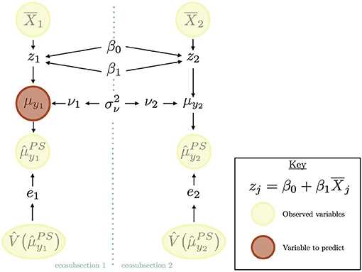
Figure 2. The area level HB estimator depicted as a PGM, which helps us understand the relationships between the data, model parameters, parameter of interest, and other key random variables. Quantities in yellow circles represent observed (known) variables. The quantity in red represents the quantity we would like to estimate. In this diagram, the quantity we would like to estimate is the mean of the response variable in the first ecosubsection. The seafoam dotted line represents the division between ecosubsection 1 and ecosubsection 2. Quantities on this dotted line represent random variables that effect both ecosubsections. The arrows represent marginal and conditional distributions of random variables.

2.3. Methods Summary

We use seven estimators–the PS estimator, two area level EBLUPs, and four area level HB estimators–to produce estimates for the average of basal area (m² per hectare), tree count per hectare, above-ground biomass (kg per hectare), and net volume (m³ per hectare). The EBLUPs and HB estimators use one explanatory variable, the average percent tree canopy cover of the ecosubsection, to produce estimates. Estimation occurs at the ecosubsection level, and thus we have produced 11,928 estimates (seven estimators, four response variables, and 426 ecosubsections). The model-based estimators are fit either within an ecoprovince or an ecosection, and hence each ecosubsection only borrows strength out to either the ecoprovince or ecosection level, not the entire IW region. In order to assess the quality of these estimators, we summarize the findings over the entire study region and for particular regions.

The data span the entire IW; however, we are forced to exclude a small portion of ecosubsections from our analyses. These ecosubsections contain either no or very close to no sampled areas with non-zero values for the variables of interest: that is, areas which are in extremely non-forested areas. These areas have to be excluded due to their within-area variance being zero or so close to zero that the software does not recognize that the number was positive.

3. Results

3.1. Estimator Performance

The indirect estimators that we implement perform similarly, on average, to the PS estimator. Figure 3 displays each indirect estimator's estimate on the y-axis and the PS estimate on the x-axis for the basal area response variable and Figure 4 does so for the count per hectare response variable. Notably, Figure 3 shows a strong linear relationship between the indirect and direct estimates (which is also observed for volume and biomass) whereas in Figure 4 this linear relationship begins to deteriorate for larger values of average canopy cover. This is due to the relationship between the explanatory variable (average canopy cover) and the PS estimator of the average tree count per hectare exhibiting more variability for those larger values, violating the model assumption of homoskedasticity. Figure 5 displays this larger variability for the tree count per hectare variable and showcases that the PS estimates consistently fall below the regression line for the largest average canopy cover values. This violation of the homoskedasticity assumption seems to have introduced bias into our indirect estimates. This represents a good cautionary tale that while indirect estimators can provide significant reductions in variance, they can be biased when the model is incorrectly specified. For the remainder of the paper, we focus on basal area, where the linear model specification seems most appropriate.

FIGURE 3

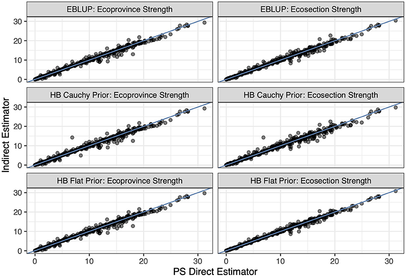
Figure 3. The six indirect estimators compared to the PS direct estimator. Each point represents two estimates of basal area for an ecosubsection, its y-coordinate representing the indirect estimate of basal area for that ecosubsection and its x-coordinate representing the PS direct estimate of basal area. The blue line is the identity line.

FIGURE 4

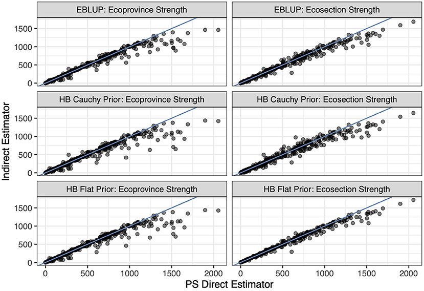
Figure 4. The six indirect estimators compared to the PS direct estimator. Each point represents two estimates of tree count per hectare for an ecosubsection, its y-coordinate representing the indirect estimate of tree count per hectare for that ecosubsection and its x-coordinate representing the PS direct estimate of tree count per hectare. The blue line is the identity line.

FIGURE 5

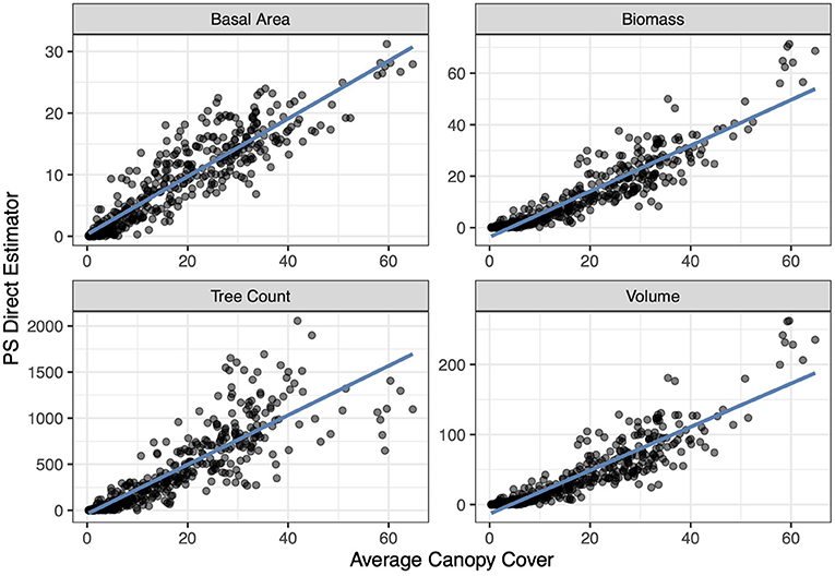
Figure 5. The relationship between the response variables and the explanatory variable (average canopy cover) for each response variable at the ecosubsection level across the IW. The x-coordinate represents the population value of average canopy cover based on remotely sensed data in a given ecosubsection, and the y-coordinate represents the post-stratified estimate of a response variable in a given ecosubsection. The blue line is the ordinary least squares regression line.

Figures 3, 4 also display that the flat prior HB estimator produces very similar estimates to the EBLUP for both the estimators that borrow strength out to the ecosection level and to the ecoprovince level. Figure 6 displays this relationship in further detail. Notably, the flat prior HB estimates and standard errors are very similar to the EBLUP. This is expected as we add no prior information to the flat prior HB estimators. By adding no information and specifying the same model we should and do see extremely similar results.

FIGURE 6

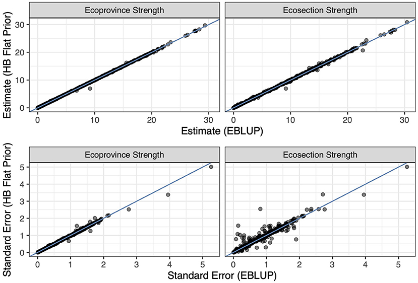
Figure 6. The flat prior HB estimators compared with the EBLUP estimators at each level of strength. The top left plot displays the estimates for each estimator at the ecoprovince level, the top right plot displays the estimates for each estimator at the ecosection level, the bottom left plot displays the standard errors for each estimator at the ecoprovince level, and the bottom right plot displays the standard errors for each estimator at the ecosection level. Each plot contains either estimates or standard errors for the basal area response variable. The blue line in each plot is the identity line.

While it is reassuring for the flat prior HB estimator to reinforce the results of the EBLUP, the full benefits of the HB estimators are not gained without careful thought into how prior information is incorporated. In our case, we specify a half-Cauchy prior with scale of one, which is considered a weakly informative prior, on the between-area variation parameter. This distribution places more probability mass over smaller values for our between-area variation, signifying that we expect the between-area variation to be low. This prior is commonly used for the between-area standard deviation parameter in hierarchical models, especially when the number of small areas is small and so the data provide little information about the group-level variance (Gelman, 2006). Further, we know that ecosections should be more homogeneous than ecoprovinces and this prior information should reinforce the homogeneity we see in the data. We still chose to place a half-Cauchy prior on the between-area variation when borrowing out to the ecoprovince level, as these regions are defined by ecologists as more homogeneous than the rest of the study region (McNab et al., 2007).

Figure 7 displays the reduction in variance when we change the prior on the between-area variation from flat to half-Cauchy in both the ecosection and ecoprovince approaches. The variance is reduced much more significantly when we use a half-Cauchy prior for estimators that borrow strength to the ecosection level because the number of small areas is smaller. In particular, one can observe that most areas where variance is reduced a large amount have less ecosubsections that they borrow strength from (light purple dots).

FIGURE 7

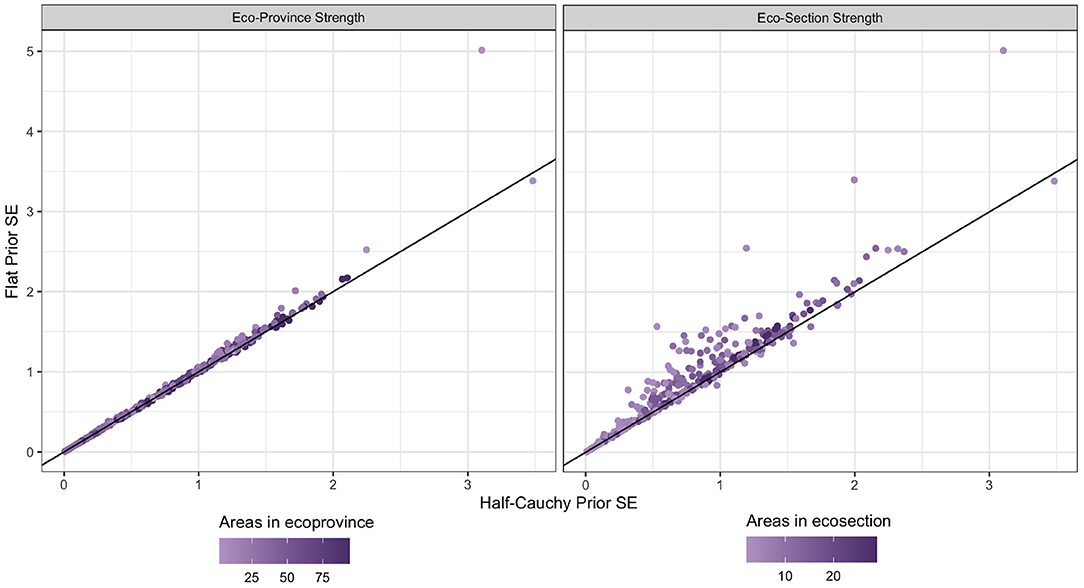
Figure 7. Basal area standard errors for each HB estimator. The x-coordinate of each dot represents the standard error when a half-Cauchy prior is placed on between-area variation, and the y-coordinate represents the standard error when a flat prior is placed on between-area variation. The color of the dot represents the number of ecosubsections that strength was borrowed out to for the given dot. The black line is the identity line. The plot on the right shows the estimators that borrow strength to the ecosection level, while the plot on the left shows the ecoprovince level estimators.

Outside of this graphical representation, we can look numerically at the mean and median percent reduction in variance when moving from a flat prior HB estimator to one with the half-Cauchy prior. Table 1 displays both the mean and median percent reduction in variance of basal area for the ecosection and ecoprovince level HB estimators. Borrowing to the more homogeneous ecosection level with the half-Cauchy prior on the between-area variation leads to the greater reductions in variance. While this reduction in variance is compelling, it is possible that the weakly informative prior introduced bias to the estimator.

TABLE 1

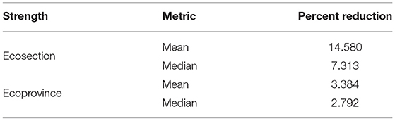
Table 1. Percent reduction in variance of basal area estimates from flat prior to half-cauchy.

To understand where bias may be introduced in our estimates, Figure 8 displays the estimates made by the HB estimators with a half-Cauchy prior compared to those made by the PS estimator, an estimator that is unbiased under resampling regardless of model accuracy. Here, we see a high level of agreement between the two estimators, which suggests the HB estimators are not systematically biased. However, it is important to note that it is the PS estimator, under resampling, that is unbiased, not a given PS estimate. We also saw strong agreement between the estimators from the half-Cauchy prior and those from the flat prior, signifying a robustness to the choice of prior distribution for the between-area variation.

FIGURE 8

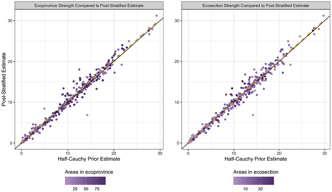
Figure 8. Basal area estimates for the half-Cauchy HB estimator and post-stratified estimator. The x-coordinate of each dot represents the estimate when a half-Cauchy prior is placed on between-area variation, and the y-coordinate represents the post-stratified estimate. The color of the dot represents the number of ecosubsections that strength was borrowed out to for the given dot. The black line is the identity line. The dashed yellow line is the ordinary least squares regression line. The plot on the right shows the estimators that borrow strength to the ecosection level, while the plot on the left shows the ecoprovince level estimators.

We can also investigate indications of bias numerically, with the percent relative difference (PRD) metric. The PRD between two estimators is defined as followed:

$PRD({\widehat{\mu }}_1,{\widehat{\mu }}_2)=\frac{{\widehat{\mu }}_1-{\widehat{\mu }}_2}{{\widehat{\mu }}_2}·100\%.$

When we examine the PRD between the PS estimator and the half-Cauchy prior HB estimator for the basal area response variable we see that the average PRDs are −0.007% and 0.756% at the ecoprovince and ecosection level, respectively. The median PRDs between for these estimators are −0.12% and −0.225% at the ecoprovince and ecosection level, respectively. The low PRD values provide additional evidence that we are not introducing much systematic bias with the use of the auxiliary data and prior on the between-area variation parameter.

3.2. Case Study: The South Central Highlands (M331G) and the Utah High Plateau (M341C)

We now explore the effects of adding prior information to the HB estimators at a micro level: by examining two ecosections. The South Central Highlands and the Utah High Plateau ecosections both exist in mountainous ecoprovinces in the IW. Figure 9 displays both ecosections. These two ecosections are located relatively close to each other in the IW, yet the addition of the half-Cauchy prior when we borrow strength to the ecosection level has a very different effect within each ecosection. To understand how the estimators perform differently across these two ecosections, we explore the mean estimates for basal area, and corresponding standard errors, within these two ecosections.

FIGURE 9

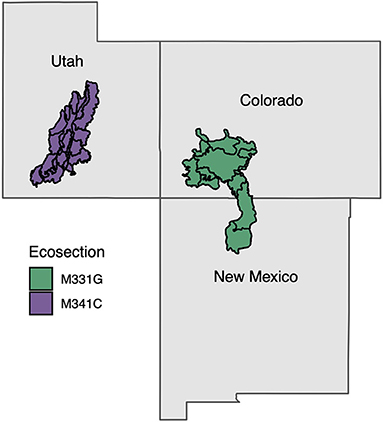
Figure 9. The South Central Highlands (M331G) and the Utah High Plateau (M341C) ecosections on a map of the three states that they collectively occupy. The purple area represents the Utah High Plateau and the green area represents the South Central Highlands. The black lines divide the ecosubsection within each ecosection.

Figure 10 displays the HB estimates and illustrates that, for both ecosections, the basal area estimate is about the same for both priors on the between-area variation parameter. This again showcases a robustness to how the prior information is specified for between-area variation.

FIGURE 10

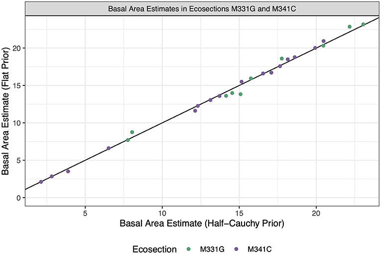
Figure 10. Estimates for each HB estimator. The x-coordinate of each dot represents the estimate when a half-Cauchy prior is placed on between-area variation, and the y-coordinate represents the estimate when a flat prior is placed on between-area variation. The color of the dot represents the ecosection that a given ecosubsection is in. The black line is the identity line.

While the estimate values show high agreement, it should be noted that the standard error estimates changed more drastically when we changed the prior on between-area variation, as seen in Figure 11. Interestingly, the standard errors in eocsection M331G are reduced significantly when the half-Cauchy prior is used compared to the flat prior, while the standard errors in ecosection M341C hardly change. This is likely due to a couple of factors. First of all, the estimated variance of the PS estimates in ecosection M331G is lower than the estimated variance of the PS estimates in M341C (32.044 and 44.384, respectively). That is, based on the data, there is less between-area variation in ecosection M331G. By placing a prior which has high probability density for small values of ${\sigma }_{\nu }^2$ we have reinforced the pattern seen in the data. Additionally, M331G is borrowing from less small areas and therefore will lean more on the weakly informative prior which preferences smaller values for the between-area variation.

FIGURE 11

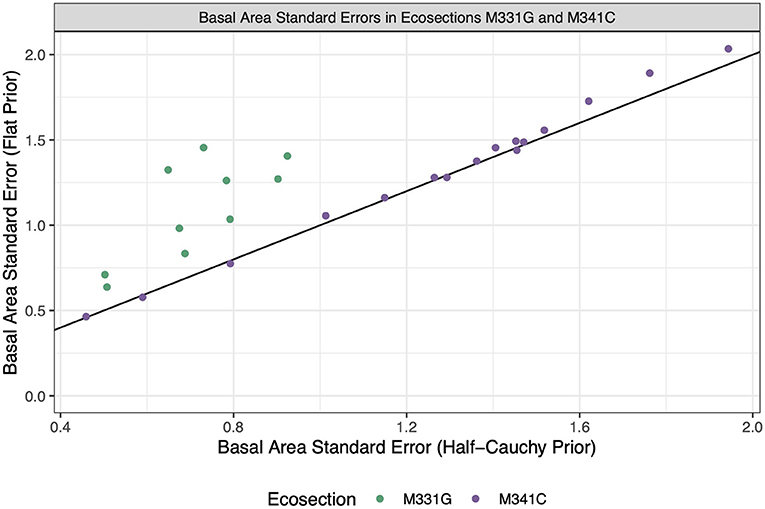
Figure 11. Standard errors for each HB estimator. The x-coordinate of each dot represents the estimate when a half-Cauchy prior is placed on between-area variation, and the y-coordinate represents the estimate when a flat prior is placed on between-area variation. The color of the dot represents the ecosection that a given ecosubsection is in. The black line is the identity line.

4. Discussion

We consider six indirect, area level small area estimators and one direct estimator across the IW region of the United States. The two HB estimators with flat priors on between-area variation mimic the two analogous area level EBLUP estimators in both estimates and variances. When supplying the HB estimators with a half-Cauchy prior for the between-area variation parameter, we see a reduction in variance when borrowing strength out to both the ecoprovince and ecosection level, with more reduction observed at the latter level of strength.

Table 2 displays the relative efficiency of each estimator implemented in this article compared the standard HT direct estimator for the basal area response variable. We define relative efficiency of a given estimator as the variance estimator of that estimator divided by the variance estimator of a direct estimator. The first column of Table 2 makes it clear that incorporating informative auxiliary data into a direct estimator, the PS estimator in this case, does improve its efficiency. These improvements mimic FIA's production process with just 2 post strata assigned at the plot level, not at the subplot level. However, greater gains can be had by moving to an indirect estimator. In particular, the HB estimator with a half-Cauchy prior on between-area variation borrowing strength to the ecosection level has the highest mean and median relative efficiency. Notably, the ecosection-level, half-Cauchy prior, HB estimators relative efficiency is greater than the ecoprovince-level, half-Cauchy prior, HB estimators relative efficiency. This gain in relative efficiency is likely due to the half-Cauchy prior being a reasonable depiction of the between-area variation of ecosubsections within a given ecosection in the IW.

TABLE 2

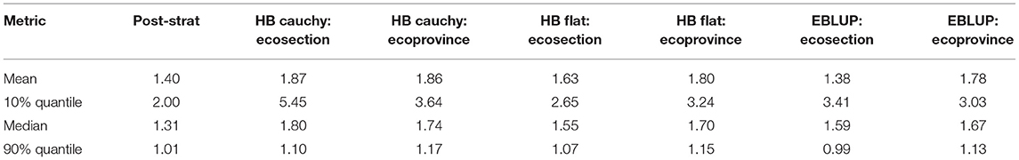
Table 2. Relative efficiency of each estimator compared to the Horvitz-Thompson (basal area response).

Figure 12 shows the relative efficiency of basal area estimates for both the ecosection- and ecoprovince-level half-Cauchy prior HB estimators compared to the PS direct estimator (as opposed to the Horvitz Thompson in Table 2). We can see more drastic improvements in relative efficiency in the more forested Northern parts of the IW, and the relative efficiency is sometimes below the PS estimator in extremely unforested areas. This might be due to artificially low variance estimates for the PS estimator, which can occur when almost all sampled units in an ecosubsection have values of 0 for the response variables. In the case of an estimator that borrows strength, such as the HB estimators, we will likely borrow strength to some areas that have larger direct estimates of response variables, giving us a larger variance.

FIGURE 12

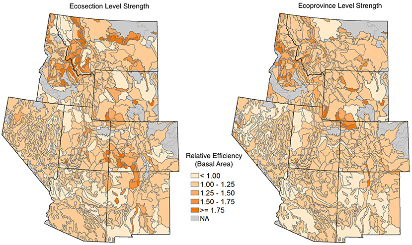
Figure 12. The relative efficiency of basal area estimates from the HB estimators with a half-Cauchy prior on between-area variation compared to the PS direct estimator. On the left, we have the HB estimator that borrows strength out to the ecosection level, and on the right, we have the HB estimator that borrows strength out to the ecoprovince level. Darker orange areas correspond to higher relative efficiency. The gray areas are ecosubsections where we were unable to obtain HB estimates.

The efficiency gains of the HB estimators with informative priors on between-area variation over the more common EBLUP and PS (see Table 2 and Figure 12) imply that these estimators can attain the same level of precision but with less sampled plots. However, the benefits of a HB approach do not stop there. Conveniently, the Bayesian paradigm allows for more intuitive inferential statements than provided by frequentist methods. Since the Bayesian methods provide a distribution for our parameter of interest, we can make probabilistic statements about the location of the parameter, whereas the frequentist approach only allows us to talk about the behavior of our method under repeated sampling.

Considering the performance and all the characteristics of these estimators, the results of this work provide some guidance on when to consider which of these estimators. If one only has a small number of areas that they borrow strength out to, and those areas are believed to have a good amount of homogeneity between them, a HB estimator with a half-Cauchy prior on the between-area variation might be preferred. On the other hand, if one has the ability to borrow strength to a large number of groups that may not be too homogeneous, keeping a flat prior on between-area variation should be considered. This suggests that the HB estimator that borrows to the ecosection level and uses the half-Cauchy prior on between-area variation may be a viable estimator for FIA applications. Further testing with alternative responses and auxiliary data in other parts of the country is warranted.

Further work will include investigations of the unit level HB estimator, particularly with an eye to handling non-Gaussian data. Researchers have explored unit level modeling of non-Gaussian data types, such as zero-inflated data (Krieg et al., 2016) and other non-Gaussian data (Parker et al., 2020a). In particular, Parker et al. (2020b) discusses the benefits of unit level models, both in terms of potential efficiency gains and incorporating various levels of spatial aggregations. We hope to investigate the utility of these unit level models in a forest inventory setting. At both the area and unit level we will also explore extensions to the HB estimators through spatially structured variance models. Ver Planck et al. (2018) explores area level HB estimators with conditional autoregressive random effects and conditional autoregressive random effects with smoothed sampling variance and found that these spatially structured variance models can help reduce the variance of the estimator. We hope to explore these spatially structured variance models further and investigate how they perform with different prior information supplied.

Data Availability Statement

The data analyzed in this study is subject to the following licenses/restrictions: the data include confidential plot data, which can not be shared publicly. FIA data can be accessed through the FIA DataMart (https://apps.fs.usda.gov/fia/datamart/datamart.html). Requests for data used here or other requests including confidential data should be directed to FIA's Spatial Data Services (https://www.fia.fs.fed.us/tools-data/spatial/index.php).

Author Contributions

GW, KM, GM, and TF: conceptualization. GW and KM: methodology and writing. GW: analysis. TF: data curation. GW and TF: data visualization. GW, KM, and GM: review and editing. All authors have read and agreed to the published version of the manuscript.

Funding

This work was supported by the USDA Forest Service, Forest Inventory and Analysis Program (via agreement 19-JV-11221638-112) and by Reed College.

Conflict of Interest

GW is employed by RedCastle Resources, Inc.

The remaining authors declare that the research was conducted in the absence of any commercial or financial relationships that could be construed as a potential conflict of interest.

Publisher's Note

All claims expressed in this article are solely those of the authors and do not necessarily represent those of their affiliated organizations, or those of the publisher, the editors and the reviewers. Any product that may be evaluated in this article, or claim that may be made by its manufacturer, is not guaranteed or endorsed by the publisher.

Acknowledgments

The authors would like to thank the USDA Forest Service, Forest Inventory and Analysis Program for the data.

References

Bechtold, W. A., and Patterson, P. L. (2005). The Enhanced Forest Inventory and Analysis Program–National Sampling Design and Estimation Procedures. USDA Forest Service, Southern Research Station.

Google Scholar

Blackard, J., Finco, M., Helmer, E., Holden, G., Hoppus, M., Jacobs, D., et al. (2008). Mapping US forest biomass using nationwide forest inventory data and moderate resolution information. Remote Sens. Environ. 112, 1658–1677. doi: 10.1016/j.rse.2007.08.021

CrossRef Full Text | Google Scholar

Boonstra, H. J. (2021). mcmcsae: Markov Chain Monte Carlo Small Area Estimation. Available online at: https://CRAN.R-project.org/package=mcmcsae

Breidenbach, J., and Astrup, R. (2012). Small area estimation of forest attributes in the Norwegian National Forest Inventory. Eur. J. Forest Res. 131, 1255–1267. doi: 10.1007/s10342-012-0596-7

CrossRef Full Text | Google Scholar

Cassel, C. M., Särndal, C. E., and Wretman, J. H. (1976). Some results on generalized difference estimation and generalized regression estimation for finite populations. Biometrika 63, 615–620. doi: 10.1093/biomet/63.3.615

CrossRef Full Text | Google Scholar

Cleland, D. T., Freeouf, J. A., Keys, J. E., Nowacki, G. J., Carpenter, C. A., and McNab, W. H. (2007). Ecological Subregions: Sections and Subsections for the Conterminous United States. Available online at: https://www.fs.fed.us/research/publications/misc/73326-wo-gtr-76d-cleland2007.pdf

Google Scholar

Coulston, J. W., Green, P. C., Radtke, P. J., Prisley, S. P., Brooks, E. B., Thomas, V. A., et al. (2021). Enhancing the precision of broad-scale forestland removals estimates with small area estimation techniques. Forest. Int. J. Forest Res. 94, 427–441. doi: 10.1093/forestry/cpaa045

CrossRef Full Text | Google Scholar

Fay, R. E. III, and Herriot, R. A. (1979). Estimates of income for small places: an application of James-Stein procedures to census data. J. Am. Stat. Assoc. 74, 269–277. doi: 10.1080/01621459.1979.10482505

CrossRef Full Text | Google Scholar

Frescino, T. S., Patterson, P. L., Moisen, G. G., and Freeman, E. A. (2015). FIESTA- an R estimation tool for FIA analysts,” in Forest Inventory and Analysis (FIA) Symposium 2015 (Portland, OR: US Department of Agriculture, Forest Service, Pacific Northwest Research Station), 72.

Google Scholar

Gelman, A. (2006). Prior distributions for variance parameters in hierarchical models (comment on article by Browne and Draper). Bayesian Anal. 1, 515–534. doi: 10.1214/06-BA117A

CrossRef Full Text | Google Scholar

Goerndt, M. E., Monleon, V. J., and Temesgen, H. (2011). A comparison of small-area estimation techniques to estimate selected stand attributes using LiDAR-derived auxiliary variables. Can. J. Forest Res. 41, 1189–1201. doi: 10.1139/x11-033

CrossRef Full Text | Google Scholar

Hidiroglou, M., and You, Y. (2016). Comparison of unit level and area level small area estimators. Survey Methodol. 42, 41–61.

PubMed Abstract | Google Scholar

Krieg, S., Boonstra, H., and Smeets, M. (2016). Small-area estimation with zero-inflated data – a simulation study. J. Off. Stat. 32:963–986. doi: 10.1515/jos-2016-0051

CrossRef Full Text | Google Scholar

Magnussen, S., Mauro, F., Breidenbach, J., Lanz, A., and Kändler, G. (2017). Area-level analysis of forest inventory variables. Eur. J. Forest Res. 136, 839–855. doi: 10.1007/s10342-017-1074-z

CrossRef Full Text | Google Scholar

Mauro, F., Monleon, V. J., Temesgen, H., and Ford, K. R. (2017). Analysis of area level and unit level models for small area estimation in forest inventories assisted with LiDAR auxiliary information. PLoS ONE 12:e0189401. doi: 10.1371/journal.pone.0189401

PubMed Abstract | CrossRef Full Text | Google Scholar

McConville, K., Tang, B., Zhu, G., Cheung, S., and Li, S. (2018). MASE: Model-Assisted Survey Estimation. Available online at: https://cran.r-project.org/package=mase

McNab, W. H., Cleland, D. T., Freeouf, J. A., Keys, J. E., Nowacki, G. J., and Carpenter, C. A. (2007). Description of “Ecological Subregions: Sections of the Conterminous United States. United States Department of Agriculture. doi: 10.2737/wo-gtr-76b

CrossRef Full Text | Google Scholar

Molina, I., and Marhuenda, Y. (2015). sae: an R package for small area estimation. R J. 7, 81–98. doi: 10.32614/RJ-2015-007

CrossRef Full Text | Google Scholar

Molina, I., Nandram, B., and Rao, J. (2014). Small area estimation of general parameters with application to poverty indicators: a hierarchical bayes approach. Ann. Appl. Stat. 8, 852–885. doi: 10.1214/13-AOAS702

PubMed Abstract | CrossRef Full Text | Google Scholar

Parker, P. A., Holan, S. H., and Janicki, R. (2020a). Computationally efficient Bayesian unit-level models for non-Gaussian data under informative sampling. arXiv [Preprint]. arXiv.2009.05642

Google Scholar

Parker, P. A., Janicki, R., and Holan, S. H. (2020b). Unit level modeling of survey data for small area estimation under informative sampling: a comprehensive overview with extensions. arXiv [Preprint]. arXiv.1908.10488.

Google Scholar

R Core Team (2020). R: A Language and Environment for Statistical Computing. Vienna: R Foundation for Statistical Computing. Available online at: https://www.R-project.org/

Google Scholar

Rao, J. N., and Molina, I. (2015). Small Area Estimation. Hoboken, New Jersey: John Wiley & Sons.

Google Scholar

Rintoul, M. A., Maebius, S., Alvarado, E., Lloyd-Damnjanovic, A., Toyohara, M., McConville, K. S., et al. (2020). “An alternative post-stratification scheme to decrease variance of forest attribute estimates in the interior west,” in Celebrating Progress, Possibilities, And Partnerships: Proceedings of the 2019 Forest Inventory and Analysis (FIA) Science Stakeholder Meeting (Asheville, NC: U.S. Department of Agriculture Forest Service, Southern Research Station), 268–276. Available online at: https://www.fs.usda.gov/treesearch/pubs/63184

Google Scholar

Särndal, C. E., Swensson, B., and Wretman, J. (1992). Model Assisted Survey Sampling. New York, NY: Springer-Verlag.

Google Scholar

Vaish, A. K., Chen, S., Sathe, N. S., Folsom, R. E., Chandhok, P., and Guo, K. (2010). Small area estimates of daily person-miles of travel: 2001 National Household Transportation Survey. Transportation 37, 825–848. doi: 10.1007/s11116-010-9279-8

CrossRef Full Text | Google Scholar

Ver Planck, N. R., Finley, A. O., Kershaw, J. A. Jr., Weiskittel, A. R., and Kress, M. C. (2018). Hierarchical bayesian models for small area estimation of forest variables using LiDAR. Remote Sens. Environ. 204, 287–295. doi: 10.1016/j.rse.2017.10.024

CrossRef Full Text | Google Scholar

Wang, J. C., Holan, S. H., Nandram, B., Barboza, W., Toto, C., and Anderson, E. (2012). A Bayesian approach to estimating agricultural yield based on multiple repeated surveys. J. Agric. Biol. Environ. Stat. 17, 84–106. doi: 10.1007/s13253-011-0067-5

CrossRef Full Text | Google Scholar

Yang, L., Jin, S., Danielson, P., Homer, C., Gass, L., Bender, S. M., et al. (2018). A new generation of the United States National Land Cover Database: requirements, research priorities, design, and implementation strategies. ISPRS J. Photogramm. Remote Sens. 146, 108–123. doi: 10.1016/j.isprsjprs.2018.09.006

CrossRef Full Text | Google Scholar

You, Y., Rao, J. N., and Gambino, J. (2003). Model-based unemployment rate estimation for the Canadian labour force survey: a hierarchical Bayes approach. Survey Methodol. 29, 25–32.

Appendix

A.1. Area Level EBLUP Variance Estimator

The variance of the Area level EBLUP is expressed by the following equation (Molina and Marhuenda, 2015; Rao and Molina, 2015):

$\begin{array}{cc}\widehat{V}({\widehat{\mu }}_j^{EBLUP})=g_{1j}+g_{2j}+2g_{3j}-b& (\mathrm{A1})\end{array}$

where

$\begin{array}{l}{g}_{1j}={\widehat{\gamma }}_j\widehat{V}\left({\widehat{\mu }}_{y_j}^{PS}\right),\\ g_{2j}={\widehat{\sigma }}_{\nu }^2{\left(1-{\widehat{\gamma }}_j\right)}^2{z}_j^{\prime }{\left({\displaystyle \sum _j{\widehat{\gamma }}_j}{z}_j{z}_j^{\prime }\right)}^{-1}{z}_j,\end{array}$

$\begin{array}{l}{g}_{3j}=2m{\left(\widehat{V}\left({\widehat{\mu }}_{y_j}^{PS}\right)\right)}^2{\left({\widehat{\sigma }}_{\nu }^2+\widehat{V}\left({\widehat{\mu }}_{y_j}^{PS}\right)\right)}^{-3}{\left({\displaystyle \sum _j}{\left({\widehat{\sigma }}_{\nu }^2+\widehat{V}\left({\widehat{\mu }}_{y_j}^{PS}\right)\right)}^{-1}\right)}^{-2},\end{array}$

$\begin{array}{l}b=2m{\widehat{\sigma }}_{\nu }^2\left({\displaystyle \sum _j}{\left({\widehat{\gamma }}_j\right)}^2-{\left({\displaystyle \sum _j}{\widehat{\gamma }}_j\right)}^2\right){\left({\displaystyle \sum _j}{\widehat{\gamma }}_j\right)}^{-3}\left(1-{\widehat{\gamma }}_j\right)\end{array}$

where

$z_j=\left[\frac{1}{X_j}\right].$

One can intuitively think about each g_#j as follows: g_1j accounts for within-area variation, g_2j accounts for variation in estimating the regression parameter β, and g_3j accounts for model-variance estimation (Hidiroglou and You, 2016).