Modeling the impacts of hot drought on forests in Texas

1 Introduction

Globally, climate change continues to exacerbate the severity, frequency and duration of drought, and forests are particularly vulnerable (Intergovernmental Panel on Climate Change [IPCC], 2013; Allen et al., 2015; Crausbay et al., 2017). In particular, tree mortality has increased due to drought across different world regions. In Europe, drought stress caused 500,000 ha of forest mortality between 1987 and 2016 (Senf et al., 2020). Besides this mortality, drought caused a substantial (between 2 and 5%) increase in defoliation, extensive dieback, and growth decline (Allen et al., 2015; Colangelo et al., 2017; Sousa-Silva et al., 2018). In the United States, drought has also been identified as a major contributor to tree mortality in California, where over 129 million trees died between 2012 and 2016 (Restaino et al., 2019). Drought-associated tree mortality is exacerbated by increasing temperatures (Williams et al., 2013; Crausbay et al., 2017; Crausbay et al., 2020). As climate warms, there have been higher magnitude and more frequent heat waves, and heat waves are expected to become even more commonplace in many regions as warming increases (van Oldenborgh et al., 2022). Thus, it is imperative to examine the combined effects of drought and extreme heat on forested ecosystems (AghaKouchak et al., 2020).

Hot drought—the co-occurrence of abnormally dry and hot conditions (Overpeck, 2013)—can cause more severe and widespread destruction of forests than drought alone (Overpeck, 2013; Schwantes et al., 2017). Evidence of this is available from many parts of the world. For instance, in the mid-2000s, ∼1.6 Pg C of biomass was reported to be either impaired or lost in the Amazon rainforest due to hot drought (Phillips et al., 2008). In the Southwestern U.S., hot drought has become a frequent occurrence, resulting in large declines of various tree species such as pinyon pines (Pinus) (Breshears et al., 2005; Pan and Schimel, 2016; Wolf et al., 2016). The projected global rise in the prevalence of hot drought has made it important to examine and, when possible, quantify the subsequent responses of forests over space and time (Frank et al., 2015).

A basic measure of forest response to stress or disturbance is tree mortality. With respect to drought or extreme heat, understanding forest response requires that relationships between climate and tree mortality are quantified based on the sensitivity and exposure of forest ecosystems (Adams et al., 2012). There is a dearth of studies on quantifiable direct measurements of tree mortality through in situ observations. Consequently, information about the immediate and long-term response of forests to drought or extreme heat is limited. We address this gap by predicting tree mortality using climate anomalies caused by high temperatures, reduced precipitation, and increased evaporative demand (Allen et al., 2015; Schwantes et al., 2017). We achieve this through statistical modeling of empirical relationships between tree mortality and climatic indices.

We focus on forests in the state of Texas, which experienced extensive tree mortality after a 2011 drought event. The 2011 drought featured some of the most extreme drought conditions ever recorded in the state. Several studies (e.g., Schwantes et al., 2017; Klockow et al., 2018) examined the effects of the 2011 drought on trees in Texas and found variable impacts. However, these studies were done over a limited area of Texas, particularly over East Texas, which is the more humid part of the state. There are insufficient studies on the impacts of droughts on forests in Central Texas, which is generally drier than East Texas, has different communities or assemblages of plants as well as distinct biomes. Because the magnitude of heat and drought was high across most of Texas, it is critical to study impacts over wider areas of the state, while acknowledging that the political boundary of Texas has no ecological relevance vis-à-vis drought impacts. Often, studies have focused on the drought (i.e., moisture deficit) aspect of the 2011 event rather than the compounding effect of extreme heat. Crouchet et al. (2019) is a notable exception in that they examined the relationship between hot drought and tree mortality, but their study was limited to 30 sites in Ashe juniper (Juniperus ashei) woodlands on the Edwards Plateau of Texas.

Capturing robust set of observations of forest conditions requires data that account for spatiotemporal variability. Some studies of drought impacts have used remotely sensed data as a measure of tree mortality (Carlson et al., 1990; Kogan, 2002; AghaKouchak et al., 2015). However, remote sensing data do not provide a comprehensive inventory of how drought effects differ by tree species or genera, tree density, basal area, diameter, or the undergrowth (Norman et al., 2016; Lawal et al., 2021). They also lack the capability to differentiate important details such as variable mortality among tree species or genera (Klockow et al., 2018). To address these limitations, an established network of field inventory that incorporates direct observations of forest composition and mortality is necessary. The Forest Inventory and Analysis (FIA) Program of the USDA Forest Service administers the U.S. national forest inventory, which collects a range of information on an annual basis that can be used to assess the status and trends of U.S. forests, including tree mortality levels (Bechtold and Patterson, 2005; Klockow et al., 2018). We used FIA data for this study because they allow for examining different tree species separately, by providing species-specific information on mortality tendencies during hot drought conditions.

To characterize and quantify meteorological drought, drought indices are typically applied (Beguería et al., 2014). These indices are broadly categorized into traditional and remote sensing derived indices (Lawal et al., 2021). Traditional indices are computed from meteorological variables, usually measured at weather stations, or from gridded data. Traditional indices are easily computed and have a relatively long record, which extends back to 1895 for (most of) the continental US. Common indices include the Palmer Drought Severity Index (PDSI; Palmer, 1965) and its derivatives (Karl, 1986) as well as the Palmer Z-Index (Soule, 1992). Limitations of these indices include their fixed temporal scale, lack of spatial precision, and their treatment of snow (Karl, 1986; Akinremi et al., 1996; Lawal, 2018). To address these limitations, the Standardized Precipitation Index (SPI; McKee et al., 1993) was developed. However, SPI is also limited because it does not account for the influence of temperature, wind, or humidity in actual or potential evapotranspiration (Teuling et al., 2013). Therefore, the multivariate Standardized Precipitation Evapotranspiration Index (SPEI; Vicente-Serrano et al., 2010; Ault, 2020) is now widely used. The SPEI is computed as a difference between precipitation and potential evapotranspiration (PET). SPEI is measured on multiple timescales and is sensitive to evaporation demand based on soil and other atmospheric and environmental factors that make plants susceptible to water stress (Hao and AghaKouchak, 2013). Nevertheless, calling SPEI or any of the aforementioned indices a drought index is something of a misnomer, as they characterize both dry and wet departures from historical moisture conditions.

Similarly, extreme heat can be represented using indices computed from meteorological variables. Regarding forest response to extreme heat, there has been increasing interest in indices related to heat waves (Breshears et al., 2021), which are defined as periods of three or more consecutive days where the daily maximum temperature exceeds a percentile threshold (commonly 90%) based on observations from a historical reference period (Russo et al., 2014, 2015). For example, the Heat Wave Magnitude Index Daily (HWMId) is an indicator that accounts for the intensity and duration of heat waves. Computed annually, the HWMId is defined as the maximum magnitude of the heat waves occurring in a year (Ceccherini et al., 2017).

Our objective in this study was to model the relationship between moisture and high temperature extremes and tree mortality for the forests of Texas. We examined the role of extreme heat in exacerbating the impacts of moisture extremes (i.e., drought) using data from FIA to assess observable tree mortality across 16 years (2004–2019). We characterized the moisture extremes using SPEI and extreme heat using HWMId. We examined relationships between these factors and tree mortality using spatiotemporal statistical models, thereby accounting for trends over time and space, as well as variations in effects based on sub-regions (East and Central Texas) and forest species composition. Our study also compared different models’ performance in examining these relationships. We investigated the following hypotheses: (1) East Texas forests are less adaptable and more vulnerable to hot drought conditions than Central Texas forests. East Texas is expected to be less adaptable because it generally has a moist climate, while Central Texas has a more arid climate. Therefore, the species assemblages in East Texas are less likely to be composed of drought-tolerant trees, and the latter represent a smaller proportion of total trees in the region; (2) Extreme heat is the principal driver of widespread tree mortality under conditions such as those observed in Texas, i.e., prolonged and intense heat waves coinciding with exceptional drought; and (3) Some trees exhibit delayed mortality during peak drought. This was informed by previous studies suggesting that oaks (in East Texas; Klockow et al., 2018) experienced mortality more quickly than other species commonly found in the region. We tested these hypotheses using a mortality index computed from the FIA data.

2 Data and methodology

2.1 Study area

We selected Texas as our study area. The FIA Program divides Texas into seven survey units (Figure 1). For this study, we focused on four of the survey units—Southeast and Northeast, and North Central and South—which we clustered into East Texas and Central Texas, respectively, for analytical purposes. We excluded the West, Northwest and West Central survey units from our study.

FIGURE 1

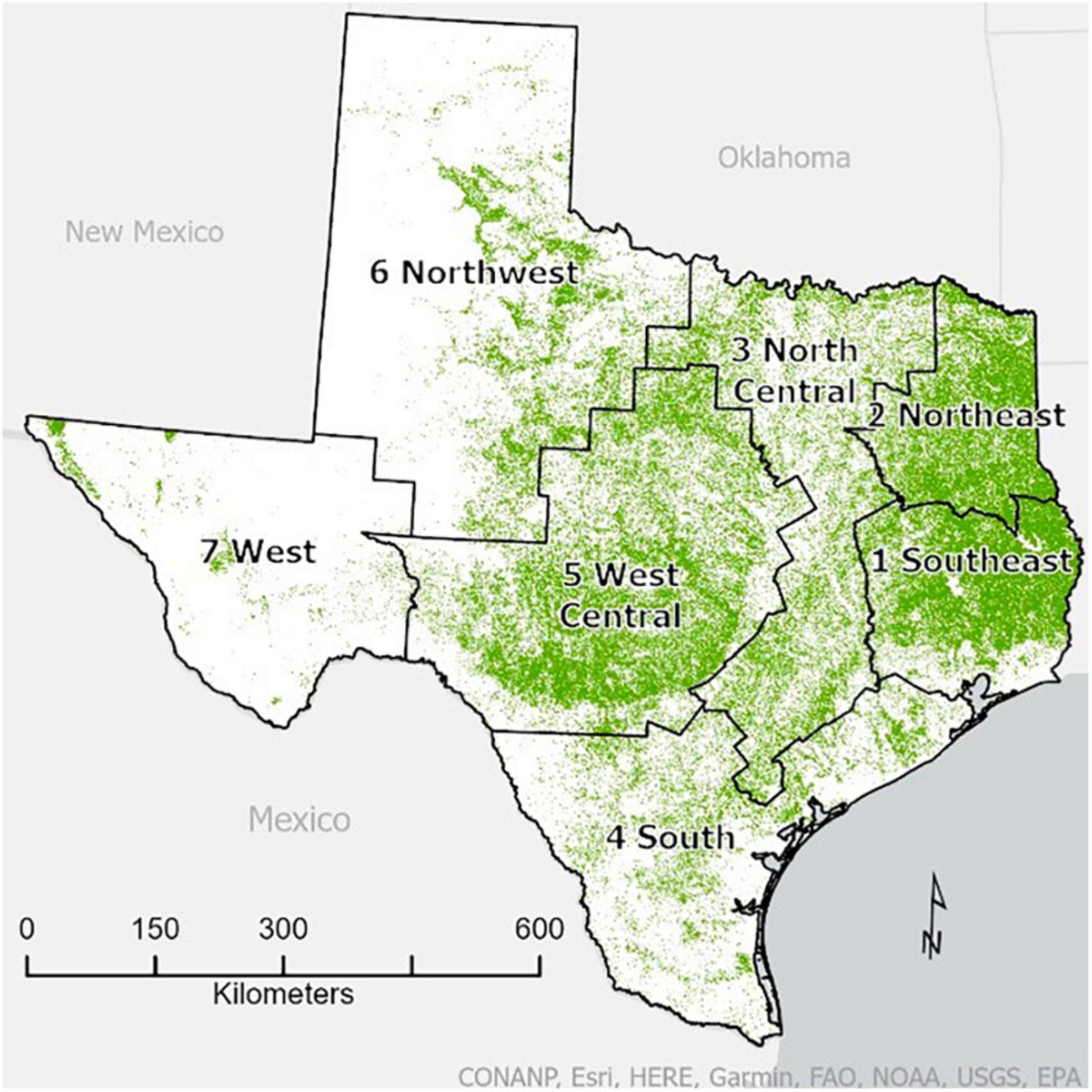
Figure 1. State of Texas showing the seven FIA survey units as well as forest cover. The map of forest cover (30-m resolution) is adapted from the 2016 USFS tree canopy cover product developed for the 2016 National Land Cover Dataset (NLCD) of the Forest Inventory and Analysis National Program (FIADB). The green pixels indicate greater than 0% tree canopy cover (i.e., a simple, binary forest mask that also captures open-canopy woodlands). The survey unit boundary map was developed from a county map available from the Forest Service’s geodata archive which is also available on FIADB.

Due to its large size and diverse geography, climatic conditions in Texas are highly varied (Kimmel et al., 2016). One defining feature is what is known as the “dry line,” which separates the humid eastern part of the state—influenced by moist air from the Gulf of Mexico—from the arid or semiarid part (Kimmel et al., 2016). In turn, precipitation follows an east-west gradient, with the mean annual precipitation ranging from 1500 mm in the east to 355 mm in the west. There is also a north-south gradient in temperature (USDA-NRCS, 2006; PRISM, 2014; National Centers for Environmental Information [NOAA], 2018).

Droughts are common in Texas. A study by the Texas Water Commission and Climate Impact Assessment found that drought is likely to occur at least once every 16 months on average (Banner et al., 2010). However, the state has experienced an increasing number of droughts and heat waves and thus is ideal for assessing drought-induced tree mortality (Schwantes et al., 2017; Deng et al., 2018).

Texas was the epicenter of a hot drought in 2011 (Crouchet et al., 2019; Klockow et al., 2020). The region experienced the driest 12 months on record during 2011, with total precipitation 410 mm (60%) less than the 20th century 12-month average (686 mm; Nielsen-Gammon, 2012; National Centers for Environmental Information [NOAA], 2018). In addition, the state experienced exceptionally high temperatures, particularly during the summer months (June-July-August), when it recorded an average temperature of 30.4°C, which was 2.9°C greater than the long-term average (Hoerling et al., 2013; Klockow et al., 2018). The historically unusual magnitude and temporal pattern (i.e., intensified to exceptional levels and dissipated relatively quickly) of these conditions have been the subject of some research (Hoerling et al., 2013; Fernando et al., 2016), but similar intense episodic events are predicted to become routine in the region and other parts of the United States (Overpeck and Udall, 2020).

Texas has 200 ecological plant communities and high tree species tree diversity (Elliott et al., 2009–2014; Subedi et al., 2021). Generally, the state’s forests and woodlands can be divided into several ecologically distinctive regions. East Texas, which encompasses the Gulf Coastal Plain and extends south toward the Gulf of Mexico, is the most densely forested region and is dominated by pines (Pinus) common throughout the southeastern U.S. (Burns and Honkala, 1990); oaks (Quercus) and sweetgum (Liquidambar) are also common (Table 1). Central Texas consists foremost of a karst landscape commonly known as “Texas Hill Country.” It is covered by a mix of closed-canopy forests and open-canopy woodlands featuring junipers (Juniperus) as well as oaks, elms (Ulmus), mesquite (Prosopis), and other deciduous species. Areas within the southern portion of Central Texas are dominated by relatively short trees (mesquite, oaks, and other hardwoods) and numerous, often thorny shrubs, although larger trees, especially certain oak species, are more common in the milder conditions near the Gulf Coast.

TABLE 1

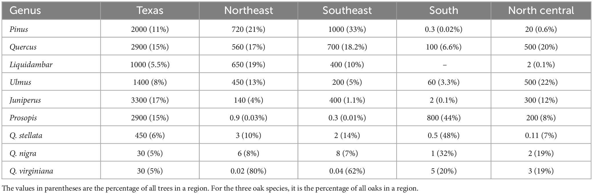
Table 1. Number of live trees (in millions) of selected tree genera and species on forest land in a survey area (Source: https://www.fia.fs.usda.gov/tools-data/).

2.2 Tree mortality

To estimate tree mortality, we used data from FIA plots across Texas. The FIA conducts an annualized survey; some plots in each state are measured every year, enabling annual estimates of forest conditions and attributes (Edgar et al., 2009).

The FIA plot design consists of a standard plot, subplots and micro-plots (Bechtold and Patterson, 2005). A standard plot comprises four 24.0 radius subplots, where trees ≥5 inches (12.7 cm) in diameter are measured. For more details about the FIA plot design, please see Bechtold and Patterson (2005). Data collected by the FIA include tree species, tree basal area (BA), diameter at breast height (DBH), recent disturbances, and status (live or dead) of the trees. Each FIA plot is associated with a geographic location (i.e., a set of x, y coordinates). Due to privacy concerns, the true locations are perturbed (i.e., coordinates are coarsened spatially) and swapped (i.e., attributes of some plots are switched with other plots). Prior studies have found that perturbing and swapping plot data did not have a significant effect on regional-scale analyses (e.g., McRoberts et al., 2005; Coulston et al., 2006), or analysis such as this where the spatial data being overlaid had a relatively coarse resolution [see section “2.3.1 Standardized precipitation evapotranspiration index (SPEI)”].

As noted earlier, the FIA program splits Texas into seven survey units (Figure 1). The FIA program uses an annualized system, where a percentage of the FIA plots in each survey unit are inventoried every year. In the Southeast (1) and Northeast (2) units, measurements of all plots in the unit (i.e., one inventory cycle) is completed every 5 years (Bechtold and Patterson, 2005). A 10-year inventory cycle is implemented in the North Central (3), South (4), West Central (5), Northwest (6), and West Texas (7) units (Bechtold and Patterson, 2005). Information that tracks the inventory cycle (and inventory year within that cycle) of a plot record allows for internal consistency. Instead, our study used the “measurement year” (i.e., the year a plot was visited) of plots as the time of observation, which provided comparable annual estimates of tree parameters across the survey units and enabled matching of the FIA estimates with indices of drought and extreme heat. We should note that a perceived shortcoming of the FIA inventory cycle is that some disturbances with localized or limited impacts are sometimes not captured promptly. However, this did not affect our model setup or findings since our focus was on widespread impacts. In our analyses, we focused on East Texas (Northeast and Southeast survey units) and Central Texas (North Central and South units) because forests in these regions are known to have been highly affected by the 2011 hot drought (Schwantes et al., 2017; Klockow et al., 2018; Crouchet et al., 2019). Moreover, the other three FIA survey units have sparser inventory data and are dominated by markedly different plant communities, with a much larger component of open woodlands is dominated by juniper species (e.g., Juniperus ashei or J. pinchotii). In addition, we examined the impacts of hot drought on six tree genera that are abundant in the target regions: pine (Pinus), juniper (Juniperus), oak (Quercus), sweetgum (Liquidambar), mesquite (Prosopis), and elm (Ulmus). Preliminary analyses suggested that oaks were among the most sensitive trees to the conditions in 2011, exhibiting mortality more rapidly than other tree genera. In turn, we also examined impacts on the three oak species that are most abundant in Texas: post oak (Q. stellata), live oak (Q. virginiana), and water oak (Q. nigra) (Klockow et al., 2018).

We estimated tree mortality over time using the ratio of dead-to-live tree basal area (hereafter, “RDA”) which is the ratio of the total basal area (BA) of standing dead trees >12.7 cm diameter at breast height (dbh) to the total BA of live trees >12.7 cm dbh, calculated per plot. The RDA was calculated directly from the FIA data. We used FIA adjustment factors to estimate these values per plot from the subplot and microplot measurements (Bechtold and Patterson, 2005). We selected RDA as an index because it is a relative measure of mortality impact at the plot level. We focused on trees with dbh >12.7 cm because that is one of the FIA criteria for recording standing dead trees, but also because we wanted to constrain the measure to larger (i.e., older) trees that are less subject to competition and other factors. This allowed us to better isolate tree mortality associated with heat and moisture conditions for the period 2004–2019. This period was selected because we wanted a time series spanning several years before and after the 2011 drought, and that was the period for which annualized FIA data were available across the state. We should note that, since we are using measurement year and standing dead tree parameters, the year of mortality observation in the FIA dataset should be reasonably close to the year when the mortality occurred.

2.3 Characterization of moisture and high temperature extremes

2.3.1 Standardized precipitation evapotranspiration index (SPEI)

We focused on meteorological drought, which is defined as a period when the magnitude of water deficit is high compared to the long-term normal in a region (Wilhite and Glantz, 1985; National Drought Mitigation Center, 2023). The primary factors that influence water deficit are temperature, wind, and humidity. We adopted a meteorological drought definition because it does not make assumptions about surface run-off and other soil attributes. In addition, we used meteorological drought because we could easily compute the associated index values from readily available data. We characterized and quantified drought using SPEI (Vicente-Serrano et al., 2010), calculated using data for precipitation (P) and potential evapotranspiration (PET) at different timescales. The timescale refers to the temporal period (e.g., 12 months) over which the monthly difference between P and PET is aggregated when computing SPEI (Table 2). As noted earlier, SPEI actually measures both wet and dry moisture extremes, although our principal interest here was in the latter.

TABLE 2

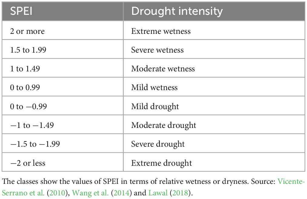
Table 2. Classes of drought intensity for the standardized precipitation evapotranspiration index (SPEI).

We used gridded daily climate data from gridMET, which have a spatial resolution of ∼4 km and spans from 1979 to present (Abatzoglou, 2013). The dataset has spatial coverage of the contiguous US; primary climatic variables include maximum temperature, minimum temperature, precipitation humidity, downward shortwave radiation, specific and relative humidity. These variables were used in the computation of reference evapotranspiration. PET was calculated based on ASCE Penman-Monteith (Abatzoglou, 2013), which is the preferred PET calculation method for use in SPEI (Beguería et al., 2014). The gridMET dataset is an interpolation of gridded PRISM data (Parameter-elevation Regressions on Independent Slopes Model; PRISM, 2014), due to its spatial attributes, and NLDAS (North American Land Assimilation System) because of its hourly temporal scale (Cosgrove et al., 2003). The gridMET datasets have been validated with weather station data and show robust agreement with observation (Abatzoglou, 2013). The gridMET data are limited in their ability to capture micro- and mesoscale features and are not well calibrated for topographic influences (Abatzoglou, 2013), although this did not affect our study because we examined broader scales. In this study, we used data for the period 2004–2019 to compute SPEI as well as HWMId, as further described below.

We computed SPEI by first subtracting PET from (Eq. 1) P. This difference is a representation of climatic water balance and is calculated at different timescales to get SPEI. Thus,

$D=\mathrm{P}-\mathrm{PET}(1)$

where D is the aggregate measurement of water surplus or deficit at a specified timescale, obtained through accumulation of individual monthly timescales. The computation of drought timescales is retrospective. For instance, a 12-month timescale is derived from the previous 12 months including the current month (Beguería et al., 2014). D-values are standardized using the log-logistic distribution to achieve acceptable statistical distribution (Beguería et al., 2014; Lawal et al., 2019b,2021, 2022). A detailed description of D-values and timescale calculation can be found in https://cran.r-project.org/web/packages/SPEI/index.html (Vicente-Serrano et al., 2010). To match the FIA data, we computed SPEI for 2000–2019 to cover important changes in trends of temporal and geographical drought coverage. We calculated 12-month SPEI (hereafter, SPEI12) and 36-month SPEI (hereafter, SPEI36). We selected these two timescales because they provide alternative depictions of the climatological phenomenon (i.e., hot drought) that triggered tree mortality. Although the start and end months of a drought (or excessively wet) event are effectively arbitrary, the 2011 drought in Texas played out over the 12 calendar months of that year: drought conditions developed in East Texas in January, spanned virtually the entire state by August and then dissipated after December because of a wet winter (Fernando et al., 2016). Thus, a 12-month timescale seemed appropriate. However, we felt a 36-month timescale was also relevant because forests typically do not show impacts unless a drought persists for multiple years (Berdanier and Clark, 2016). Additionally, we considered including 24-month SPEI, but preliminary analyses revealed that it was highly correlated with SPEI12 and SPEI36 and therefore unlikely to contribute much unique information to our models. We plotted the spatial distributions of SPEI12 and SPEI36, and then calculated their time series by decomposing them into three components: trend, seasonality, and noise.

We should note that we looked at SPEI12 and SPEI36 in the years prior to the RDA measurement year. This is under the assumption (borne out by literature) that tree mortality is lagged relative to SPEI (or HWMId). We also acknowledge that there is some noise in the mortality signal due to background mortality and mortality due to other larger-scale disturbances (e.g., fire).

2.3.2 Heat wave magnitude index daily (HWMId)

The HWMId provides a straightforward way to characterize the relative importance of extreme heat during a given year in different regions. The HWMId is computed from the Heat Wave Magnitude Index (HWMI), the number of heat waves with durations greater than or equal to three consecutive days above a daily temperature threshold, with 1981–2010 as the reference period (Russo et al., 2014). The reference period follows what was used in previous studies. The threshold is described as the 90th percentile of the daily maximum temperature distribution over a 31-day window (Russo et al., 2014) (Eqns. 2, 3).

$A_d=\bigcup _{y=1981}^{2010}\bigcup _{i=d-15}^{d+5}{T}_{y,i}(2)$

where ⋃ denotes the union of sets and T_y,i is the daily maximum temperature of the day i in the year y.

The HWMId is then calculated as the sum of the magnitude of consecutive days comprising a heat wave, with the daily magnitude computed as

$M_d(T_d)=\{\begin{array}{cc}\hfill \frac{T_d-T_{30y25p}}{T_{30y75p}-T_{30y25p}}\mathit{\hspace{1em}}\hfill & \text{if}{T}_d>T_{30y25p}\hfill \\ \hfill 0\mathit{\hspace{1em}}\hfill & \text{if}{T}_d\le T_{30y25p}\hfill \end{array}(3)$

Where “T_d is the maximum daily temperature on day d of the heatwave, and T_30y25p and T_30y75p are, the 25th and 75th percentile values, respectively, of the time series composed of 30-year annual maximum temperature within the reference period 1981–2010. The slope of the M_d(T_d) is defined at each specific location depending on T_30y75p and T_30y25p which are different in places with different climates” (Russo et al., 2015). Table 3 shows the categories of HWMId. These categories were considered in the model and summarized in figures below. We computed HWMId from gridMET data for the 1981–2019 period over Texas.

TABLE 3

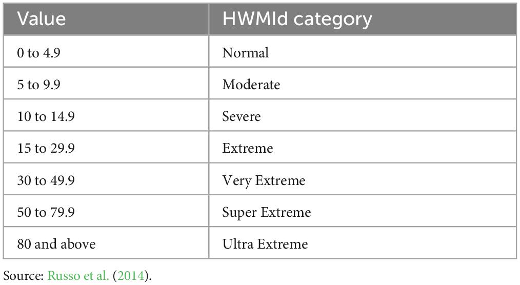
Table 3. Categories of HWMId (Russo et al., 2014).

2.4 Statistical analyses of tree mortality response to moisture and heat extremes

To estimate the contribution of moisture extremes (i.e., drought) and extreme heat to tree mortality, we used two statistical methods: gradient boosting regression (GBR) and generalized additive models (GAM). GBR is a machine learning model that can assess a non-linear relationship between a target variable and other features. It provides better accuracy than most other statistical models (such as logistic regression), requires minimal data for pre-processing, is highly flexible and handles missing data well in model fitting (Prettenhofer et al., 2014). We used GBR to predict tree mortality based on SPEI12, SPEI36 and HWMId as independent variables. We used GBR to build a base model to predict observations. We excluded FIA plots where there were only dead trees as those trees may have died before the period of interest. Preliminary analyses showed that, there was only one plot each in 2009 and 2015 where there were no live trees. We transformed the data using StandardScaler, which ensures that the variables were treated equally and not given higher weight relative to other variables (Raju et al., 2020). StandardScaler eliminates biases in predictions by scaling the data (e.g., mean is 0 and the standard deviation/variance is 1) (Raju et al., 2020). GBR is a combination of multiple models (also known as base estimators or weak learners) to produce final predictions. This allows for the combined model to capture various signals from the variables.

We evaluated the GBR results to assess their capacity to predict tree mortality response successfully based on the predictors. While we were confident that the mortality was associated with moisture deficits rather than surpluses, the predictors in question (SPEI12 and SPEI36) depict departures across the moisture gradient (wet to dry).

GAM is a linear model that can learn non-linear relationships. GAM does not limit the relationship between variables and models the outcome through summation of arbitrary functions of individual features. This type of flexible function is known as a spline or, in the GAM context, a “smooth” function. Qualitatively, the difference in the two models is particularly in terms of focus on the predictor (GBR) vs. maximizing explained variance (GAM). We should note that the partial dependence plot is a representative of variable influence (i.e. SPEI and HWMId) on the response variable (i.e. RDA) and not representation of the values. Therefore, the negative numbers on the y-axis are not raw probabilities but those of probabilities logits. While GBR reduces over-learning or overfitting to increase predictive performance, for GAM, there is freedom in reducing the multicollinearity effect (Elith et al., 2006; Leathwick et al., 2006). In simpler terms, we applied GAM to increase the robustness of our findings by confirming the results of the GBR model. Similar to GBR, we predicted tree mortality using SPEI12, SPEI36 and HWMId as predictors and RDA as the response variable. To compare our GBR and GAM results, we used the mean absolute error (MAE). The MAE measures the average absolute magnitude between observed (actual) and predicted values by the model.

3 Results

3.1 Temporal variability of tree mortality

The dead-to-live ratio (RDA) varied across the different regions of Texas (Figure 2). Generally, there was a higher median RDA between 2011 and 2013, similar to the findings of Moore et al. (2016). Over East Texas (both Southeast and Northeast survey units, Figures 2A, B), the median RDA trend was largely negligible between 2004 and 2010, before increasing from 2011 to 2014. For South Texas (Figure 2D), the trend increased between 2014 and 2015. In North Central Texas (Figure 2C), there was another increase in median RDA in 2016. It should be noted that the 90th percentile of RDA is higher for Central Texas (i.e., North Central and South units) than East Texas, even though the median of the latter is higher, as shown by the percentage of RDA in Supplementary Figure 1.

FIGURE 2

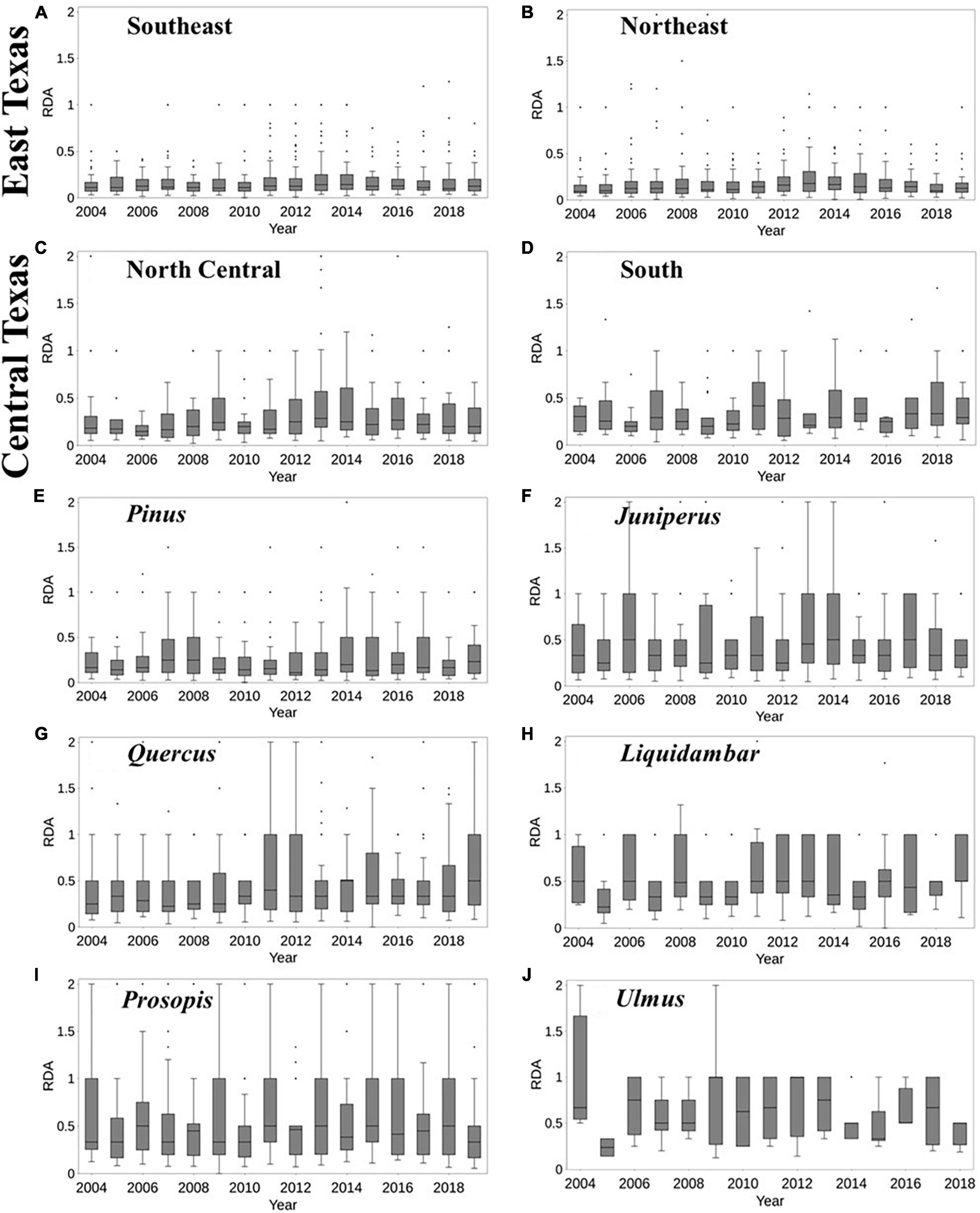
Figure 2. Temporal variability of tree mortality over Texas survey units, including Southeast and Northeast (East Texas) and North Central and South (Central Texas) (A–D), and genera (F–J) for the period 2004–2019. Data on dead trees were scant for Ulmus spp for 2019. The percentages of dead trees in each year are shown in Supplementary Figure 1. The boxplots show the minimum, 25th percentile, 50th percentile, interquartile range, maximum values, and outliers of RDA.

There was tree genera variability in RDA across years (Figures 2F–J). Juniperus, Liquidambar, and Prosopis mostly had the highest median RDA (about 0.5) between 2011 and 2013. In 2014, about 75% of Quercus plots had an RDA of 0.5 which was the largest value for the period 2004–2019. Pinus had a considerable increase of RDA during 2013–2014, however, it had the lowest RDA in 2012. On the other hand, Liquidambar exhibited a large drop in RDA in 2005, which was unique to the genus. Quercus had the longest increasing trend in RDA (2007–2010) in comparison to other genera. For Ulmus, there was similarity in the tree mortality for the period 2011–2014. The variation among genera and in different years across regions suggest highly variable responses by Texas forests to drought, extreme heat.

3.2 Temporal evolution of drought and heat wave magnitude

The trends of SPEI12 and SPEI36 were similar and largely increased between 2000 and 2005, thus suggesting increasing wetness for the period (Figures 3A, B). However, wetness declined from 2008 to 2014, suggesting an increasing intensity of drought (Figures 3A, B). The years 2011–2013 had the lowest values for SPEI at both timescales. Although the pattern of variability is similar for East and Central Texas, the magnitudes differ. The spatial magnitudes of SPEI are also depicted in Supplementary Figures 2, 3, which show that, for 12-month SPEI, extreme drought (< −2) was more commonly observed in East Texas (2011–2013).

FIGURE 3

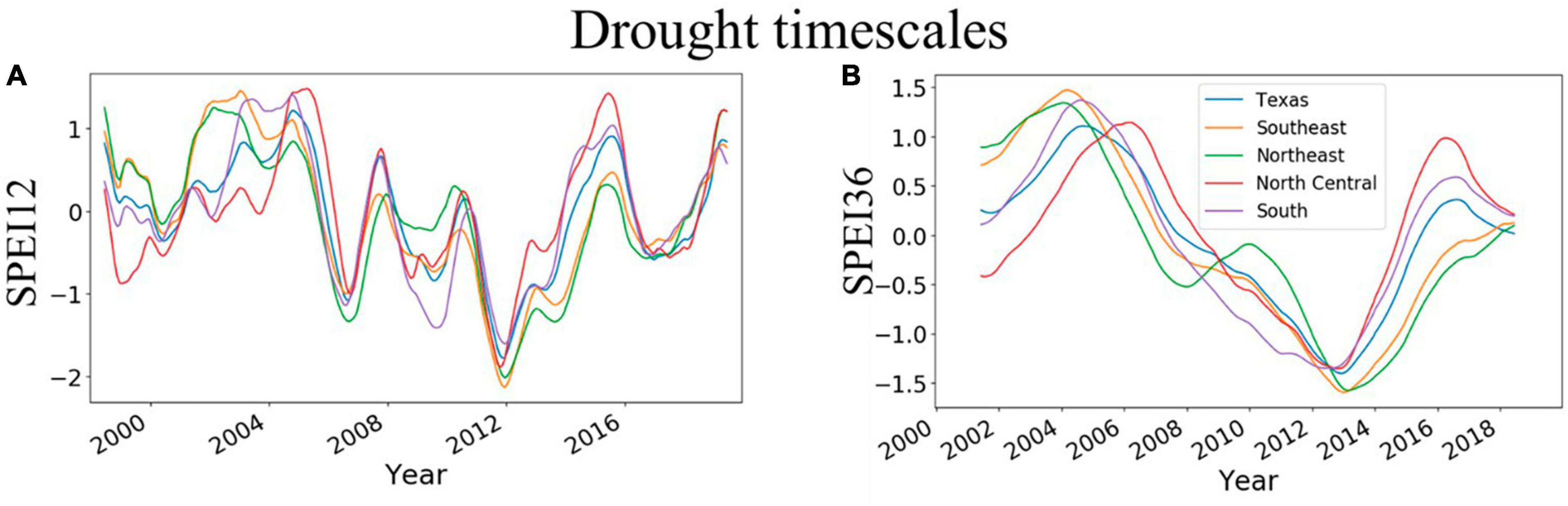
Figure 3. Temporal evolution of 12- and 36-month drought timescales across Texas and individual survey units in East Texas (Southeast and Northeast) and Central Texas (North Central and South). (A,B) Show trends of 12- and 36-month SPEI, respectively. The 12-month timescale is derived from the previous 12 months including the current month while 36-month timescale is derived from the previous 36 months including the current month.

Heat wave magnitude, as measured by HWMId, was higher in 2011–2013 than at any other time in the 2004–2019 analytical period (Figure 4). The Southeast, Northeast and North Central survey units experienced ultra-extreme (HWMId > 80) heat wave magnitudes during these three years. Among these units, the Southeast and Northeast (i.e., East Texas) experienced the highest magnitudes, while the South experienced the lowest magnitude. East Texas and part of the semi-arid region (i.e., North Central) falls in super extreme or ultra-extreme HWMId categories. Although the conditions were not nearly as bad as in 2011–2013, East Texas also had extreme heat wave magnitude in 2015–2016. Supplementary Figure 4 shows the spatio-temporal distribution of HWMId over Texas survey units.

FIGURE 4

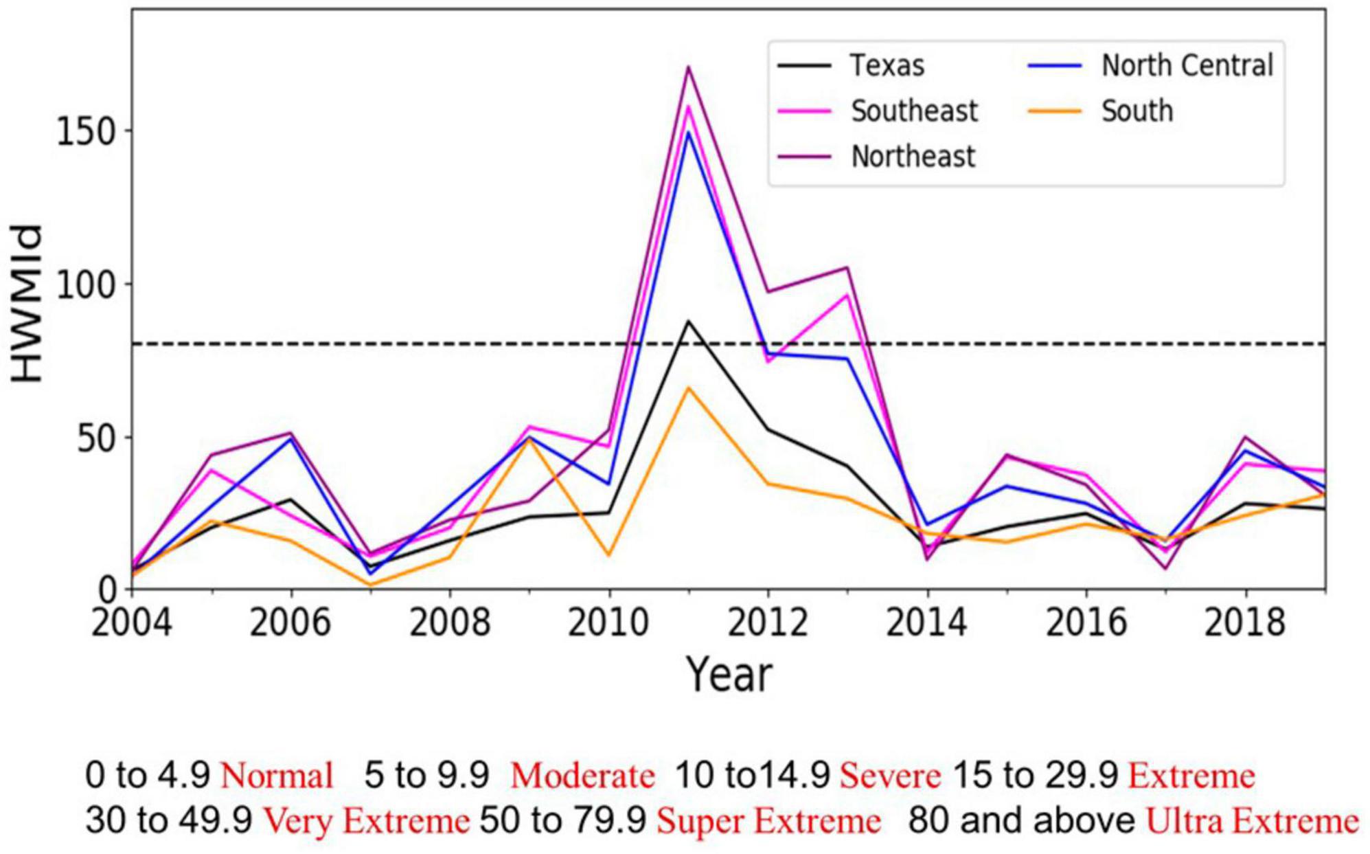
Figure 4. Time series of Heat Wave Magnitude Index daily (HWMId) in Texas and across the Southeast and Northeast survey units (East Texas) as well as the North Central and South units (Central Texas). The dashed black line (HWMId > 80) delineates the ultra-extreme. HWMId category (see Table 3). Supplementary Figure 5 shows HWMId values for an extended period and for all seven Texas survey units, while Supplementary Figures 6, 7 show spatial distributions of a mixture of drought and extreme heat.

3.3 Statistical modeling of forest ecosystem response to drought and heat waves in east and central Texas

The impacts of drought and heat waves on forest mortality is illustrated in the relationship between the predicted and observed RDA from gradient boosted regression (Figure 5). Here, we used SPEI12, SPEI36 and HWMId as predictors of tree mortality as measured by RDA. SPEI36 had a stronger relationship than SPEI12 or HWMId. Except for the South survey unit (Figures 5D–H), where HWMId was most important, SPEI36 was largely more influential than the other variables. In the same vein, SPEI12 was the least influential factor except for in the South (Figure 5H). The largest correlation (r = 0.97) between observed and predicted mortality (i.e., observed and predicted RDA) was also in the South survey unit (Figure 5H).

FIGURE 5

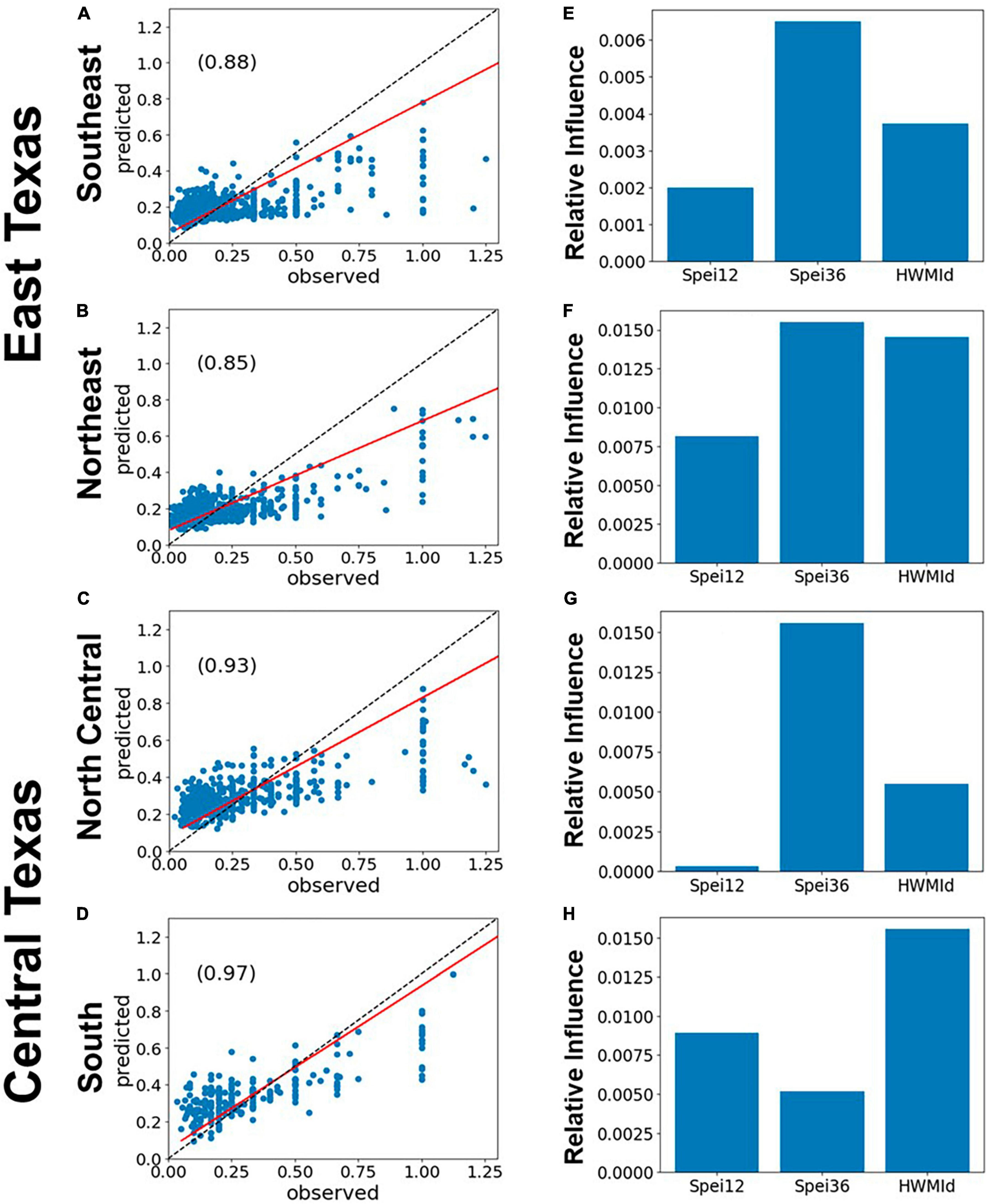
Figure 5. Performance of gradient boosted regression (GBR) models of tree mortality as represented by RDA, using 12- and 36-month SPEI and HWMId as predictors, for East and Central Texas. The left panels (A–D) show the scatterplots of model fit (predicted vs. observed) and the r-values (inset), while the panels on the right (E–H) show the relative importance of the predictors. The red line is the regression line while the dashed black line is the 1:1 line. The evaluation results are shown in Table 1 while the model results of the relationship between individual independent variables and RDA are given in Supplementary Figures 8–10.

For the six selected tree genera, the correlations between observed and predicted mortality were generally high (r ∼ 0.97). Typically, peak tree mortality occurred after moisture deficits rather than surpluses (see Figures 2E–H). When combined with the presence of extreme heat, this suggests a strong association between mortality and hot drought conditions (Figure 6). The model set-up of predictors and RDA is given in section “2.4 Statistical analyses of tree mortality response to moisture and heat extremes.” In short, the impacts of HWMId on tree mortality outweighed those of SPEI12 or SPEI36 for all genera, except oak (Quercus), for which SPEI36 played a dominant role. Notably, with respect to the three oak species, HWMId was the most influential for post oak (Q. stellata) and live oak (Q. virginiana), while SPEI12 was most influential for water oak (Q. nigra) (Figure 7).

FIGURE 6

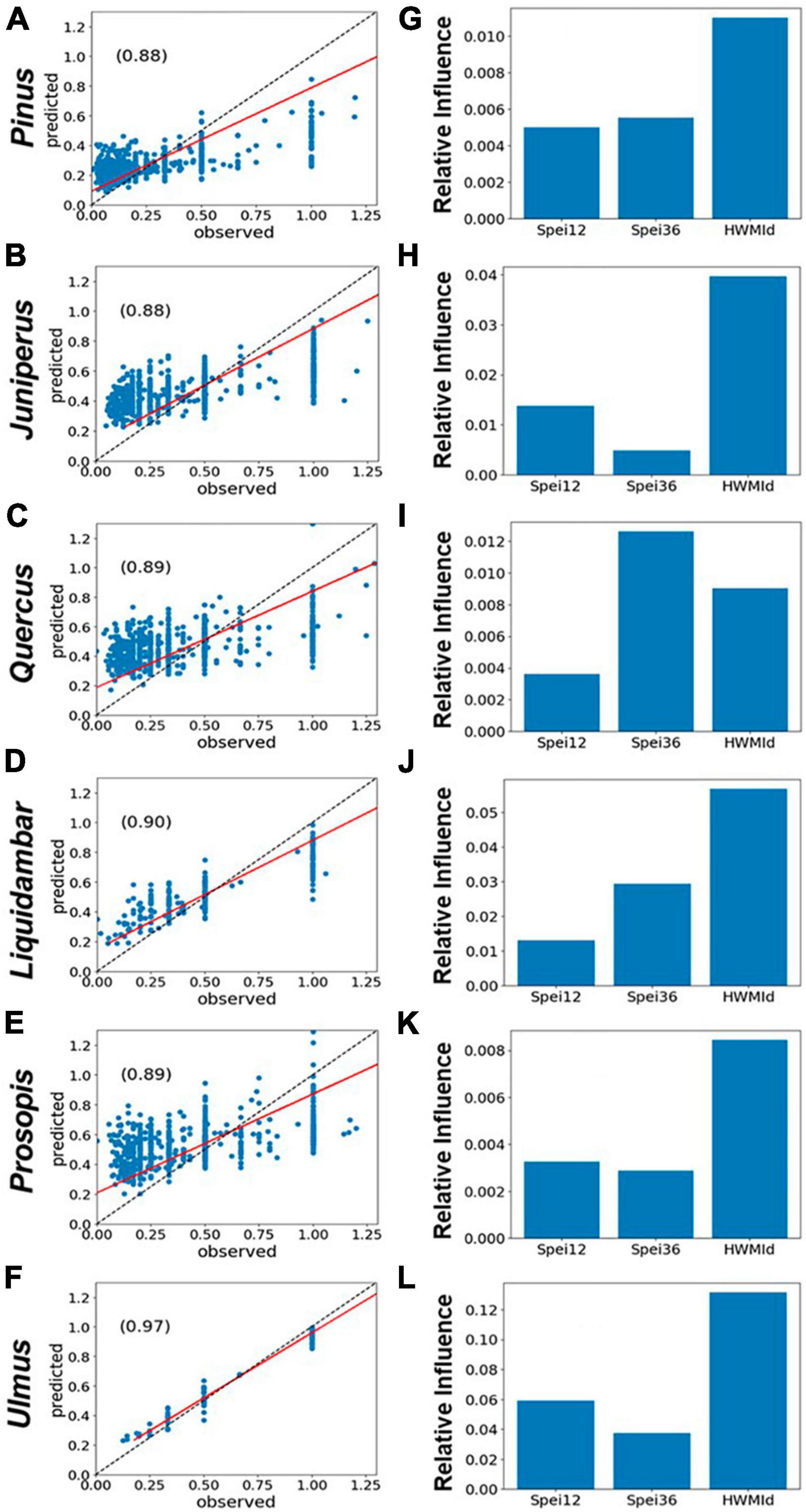
Figure 6. Performance of gradient boosted regression (GBR) models of tree mortality as represented by RDA, using 12- and 36-month SPEI and HWMId as predictors, for East and Central Texas. (A–F) The left panels show the scatterplots of model fit (predicted vs. observed) and the r-values (inset), while the panels on the right (G–L) show the relative importance of the predictors. The red line is the regression line while the dashed black line is the 1:1 line.

FIGURE 7

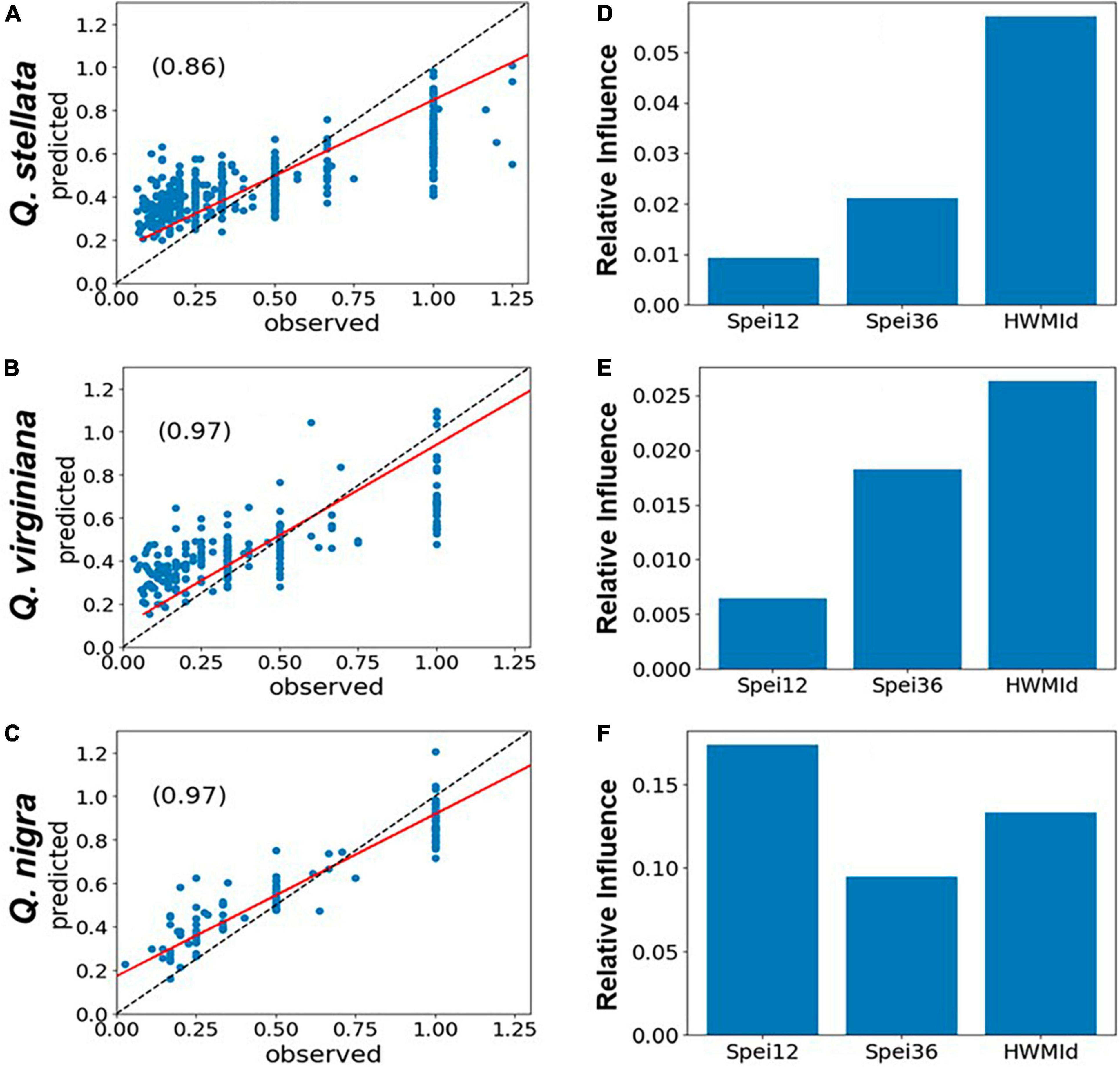
Figure 7. Post oak (Quercus stellata), live oak (Q. virginiana) and water oak (Q. nigra): Performance of gradient boosted regression (GBR) models of tree mortality as represented by RDA, using 12- and 36-month SPEI and HWMId as predictors, for East and Central Texas. The left panels (A–C) show the scatterplots of model fit (predicted vs. observed) and the r-values (inset), while the panels on the right (D–F) show the relative importance of the predictors. The red line is the regression line while the dashed black line is the 1:1 line.

GAM results were largely consistent with the GBR results, so most of the former results are only shown in the Supplementary Information. Figure 8 shows only the marginal effect results for the tree genera (i.e., the contribution of the marginal impacts of each predictor to tree mortality). Supplementary Figure 11 shows GAM outputs for Quercus species. Note that each partial dependence plot represents the influence of a predictor on RDA and is not a representation of the values. We should also note that the larger the range of the feature values, the more dominant the influence of a predictor. In this case, for most of the genera, we observe a higher impact on RDA when SPEI12 was between 0 and −0.5 but a reduced impact when SPEI12 was lower (≈−1). For Liquidambar, there was very little change in the impacts of SPEI12 at different magnitudes. On the other hand, for Pinus and Quercus, the marginal impact of SPEI12 was higher when the drought magnitude was greater (i.e., when SPEI12 was more negative), and for Quercus in particular, when SPEI12 was −1 or less,. This implies that Quercus was more affected by the greater magnitude of the 12-month drought (i.e., lower values of SPEI12) than the other genera. For SPEI36, there was a higher marginal impact on Pinus and Quercus when SPEI36 fell between 0 and −0.5. For Juniperus the marginal impact was higher when SPEI36 values were less than −0.5. For Prosopis, the marginal impact was higher when SPEI36 was about −1. In the case of HWMId, mortality response was variable to the heat wave magnitude for different tree genera. For example, the highest marginal impact of heat wave magnitude occurred when HWMId was ∼ 50 for Pinus and Liquidambar, suggesting that the genera were most susceptible during extreme heat. However, for Juniperus, the greatest susceptibility occurred during ultra-extreme heat, i.e., when heat wave magnitude was exceptionally high.

FIGURE 8

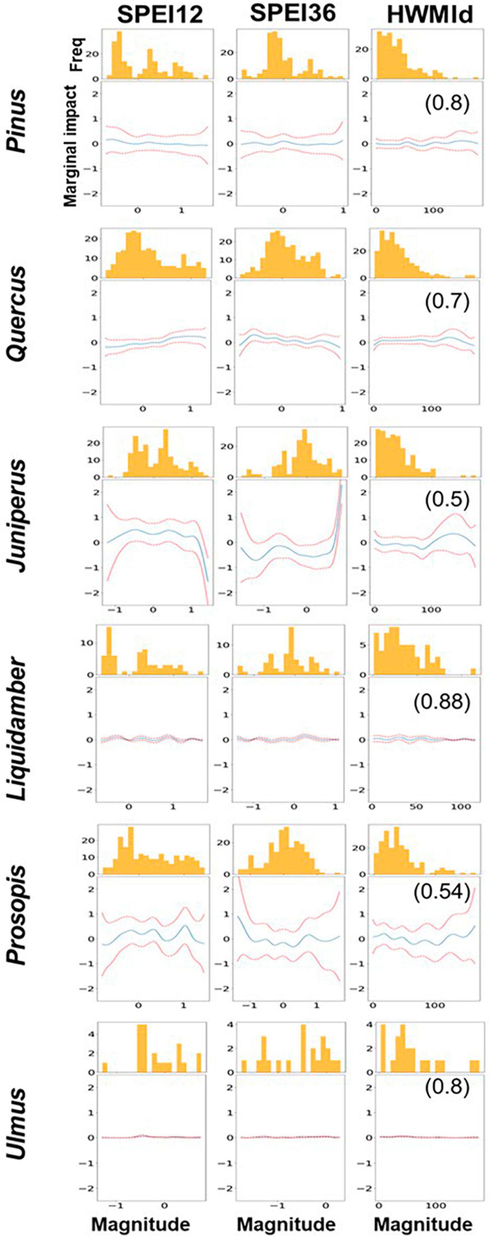
Figure 8. Partial dependence effects of SPEI12, SPEI36, and HWMId on tree mortality. The r-value is given in brackets on the right panels. Summary statistics of Generalized Additive Model (GAM) are shown in Supplementary Table 1. The y-axis shows the degree of partial dependence while the x-axis plots the predictions i.e., 12-month SPEI (SPEI12), 36-month SPEI (SPE36) and heat wave (HWMId). The histogram shows the distribution of observed RDA, which displays the intervals (bins) and frequency of count of data points that fall in each interval. It provides insight into how RDA values are distributed across different ranges of each feature and how the partial dependence plots are influenced by variations in RDA.

We also show the evaluation of the models with MAE. Generally, GBR performed much better (with lower MAE) than GAM (Table 4).

TABLE 4

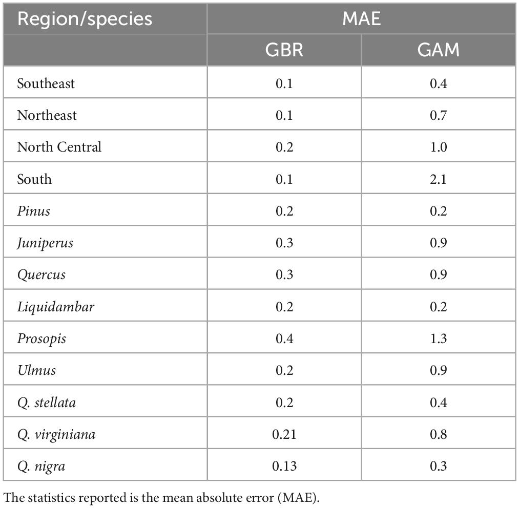
Table 4. Results of evaluation of statistical performance for the GBR and GAM models.

4 Discussion

4.1 Tree mortality and risk to forest ecosystems of hot drought in Texas

We examined relationships between moisture extremes (principally drought), heat, and forest mortality across a large portion of Texas that spans a range of ecoregions, physiographic characteristics, and forest communities. We found that there was a strong mortality signal in humid East Texas, and the relationship between this mortality and hot drought conditions is a robust finding. This finding was consistent with other research (Klockow et al., 2018; Subedi et al., 2021; Chaudhary et al., 2023), but it is important to note that most previous studies regarding the 2011 drought event focused exclusively on East Texas. Notably, we found drought-related mortality signals in semiarid Central Texas, too. Moore et al. (2016) also looked across all of Texas and they argued that East Texas did not have higher mortality as a percentage of all trees; rather, it was central Texas that saw the greatest percent mortality.

We showed the risks to Texas forests from the 2011 event. We found that tree mortality across the region was associated with the magnitude of both heat and moisture extremes (Figures 2, 5 and Supplementary Figure 2). Our findings are mostly in agreement with previous studies (Moore et al., 2011; Moore et al., 2016; Klockow et al., 2018). Although many endogenous (e.g., stand characteristics, soil properties) and exogenous (e.g., climate-related) factors contributed to these impacts, drought has been identified as the primary cause (Elkin et al., 2015; Saud et al., 2016). The combination of these factors (such as longer hydraulic paths and increased atmospheric demand) likely explains some of the variation in temporal variability of tree mortality among species (Figure 2). Also, there are many other factors (including tree physiology) that influence species’ susceptibility to drought (Seleiman et al., 2021), thus there is variability in mortality among species. Nevertheless, we found mortality trends increased rapidly in relation to a combination of drought and extreme heat (i.e., hot drought). We note that, with respect to tree mortality in Texas, heat waves have not really been considered in previous research.

Mortality was especially prominent in East Texas. However, drought conditions were not appreciably more intense in East Texas than Central Texas. The hypothesis that East Texas is less drought-adapted than Central Texas and therefore more vulnerable to drought-induced tree mortality is not definitely supported in our analysis, but it is not fully refuted, either. Our alternative hypothesis is that what most distinguished East Texas from the rest of the state was the significantly higher heat wave magnitudes in 2011. This overrode any variation in drought tolerance among the dominant tree genera in East Texas. The heat wave magnitudes in East Texas in 2011 were substantially higher than anywhere else in the state. Moore et al. (2016) observed greater mortality of larger trees in East Texas and posited that this was because the canopies of taller trees are more exposed in this region and therefore more vulnerable to high temperature extremes and associated vapor pressure deficits. In summary, our data and models point to extreme heat as a contributing factor. Thus, the impact of hot drought, an extreme event, to tree mortality is elucidated, and the hypothesis is supported in this study.

4.2 Variations in the response and adaptive mechanisms of trees to hot drought

This historically exceptional event could be an indication of future climate conditions where hot drought not only becomes more frequent but more intense in Texas. For example, we showed that pines, the predominant tree genus in East Texas, endured the event better than most other genera in the region. This is consistent with the findings of Schwantes et al. (2017). In addition, we showed that drought impacts were lagged for pines relative to oak and sweetgum, both of which are prominent in East Texas. A study by Klockow et al. (2018) similarly showed a lag in mortality for loblolly pine (P. taeda) compared to sweetgum (L. styraciflua), winged elm (U. alata), and three oak species (Q. falcata, Q. nigra, and Q. stellata) in East Texas. Besides mortality lagging for species of pine, some studies have revealed lower mortality overall, which may be attributed to effective management (including fertilizing, thinning, prescribed burning as well as reduced competition) and the capacity of the species to succeed under a broad range of conditions (Fox et al., 2007). Bottero et al. (2017) and Gleason et al. (2017) reported that, across Texas, pine species benefit from active thinning and stand density reduction because these activities mitigate water stress. With regards to the mechanisms for reducing water stress, pines preserve a high leaf water potential and reduce leaf surface area, i.e., an isohydric water conservation approach. These mechanisms may have permitted the lagging of mortality due to the 2011 drought conditions (Maggard et al., 2016). Another physiological process of pines that could manifest as delayed mortality is the disconnection of roots from the soil to conserve the leaf water potential, which may allow the trees to appear as alive with green needles even though they are unable to reconnect to the soil; in turn, the trees may appear to die (turn brown and lose needles) later even if there is subsequent rainfall (Li et al., 2022; McDowell et al., 2022). We posit that the disconnection might occur because pines do not actively maintain the connection and the delayed mortality is a consequence of that. Regardless of mechanism, the significant mortality of pines after two years suggest that the 2011 drought was so severe that it caused trees to suffer low rigor, terminal hydraulic damage, and carbon depletion (Anderegg et al., 2013; Berdanier and Clark, 2016). Perhaps because it was a hot drought, the pines—which may have been able to tolerate drought for months or even years under different circumstances—eventually were overcome by the added physiological stress caused by extreme heat.

The impacts among the hardwood genera were varied. For example, like Klockow et al. (2018) we found that oaks were most readily impacted by—and therefore most vulnerable to—the extreme conditions that occurred in 2011. Generally, we can attribute this impact to water use efficiency of the oaks. The three oak species on which we focused, live oak (Q. virginiana), water oak (Q. nigra), and post oak (Q. stellata), all experienced considerable mortality. This decline may be attributable to these species experiencing negative water balance and transpiration beyond a sustainable threshold due to drought, thus leading to hydraulic failure and making them anisohydric plants; and an inference that as drought become more severe under a changing climate, oaks are among the most vulnerable (Adams et al., 2012; Cailleret et al., 2017; Rodríguez-Calcerrada et al., 2017). Other species such as sweetgum (L. styraciflua, the only North American species in the genus) showed mortality from 2011 but peaked two years post-drought (Figure 2I). Since sweetgum is an isohydric species, this attribute may have enabled sweetgum to have longer-term resistance to drought (Esperon-Rodriguez and Barradas, 2015; Klockow et al., 2018). A possible explanation for the eventual vulnerability of sweetgum, particularly in East Texas may be that it was outcompeted (since it is an intermediate species in the region) by pines which are more dominant (Burns and Honkala, 1990). Similar to pines, sweetgum trees may also disconnect from the soil but appear as “living” plants because they still store water in their tissue. Thus, while mortality might start during peak drought, it becomes visible later when the plant reconnection to soil revives other species. Our study offers evidence affirming the notion (and hypothesis) of delayed mortality in some isohydric species such as pines and sweetgum, so we think that possible mechanisms such as the disconnection of roots from soil may be fruitful subjects of future research. It may be also worth noting, however, that sweetgum is a stump-sprouter and can regenerate more easily than oaks, the other dominant hardwoods in East Texas.

The tree mortality of some species was attributed to secondary stressors by the FIA. Several studies (e.g., Anderegg et al., 2013; Kolb et al., 2016) have also found that the susceptibility of some trees to pests is a result of the aftermath effect of drought.

4.3 Variability in regional response to hot drought

We found spatial variation in the response to hot drought across Texas and this reflects a combination of underlying factors. Foremost, the regions have different forest types and dominant tree species, as already noted. Physiological attributes (mesophytes vs. xerophytes or hydrophytes) substantially determine how plants respond to drought, so the regions’ characteristic species assemblages are likely to show some level of variation. Some of the differences are probably related to forest ecological dynamics. For example, East Texas forests have greater biomass and more shade-tolerant species, thus suggesting that successional dynamics do not play a major role in the response (van Mantgem et al., 2009; Schwantes et al., 2017). We must acknowledge that dissimilarities in response between East Texas and elsewhere in the state might be confounded by the contrasting FIA inventory cycles of the two East Texas survey units vs. the units in Central (and West) Texas, as the plots are visited half as frequently in the latter. Nevertheless, there are several factors that one would expect to affect regional variation in response. Of course, for instance, studies have shown that the general moisture regime of a region can play an important role in mortality of trees and other plants. We should point out that vapour pressure deficit (VPD) could be playing a role in South Texas. We should note that extreme heat (as measured by HWMId) observed in South Texas was still high at about 52 and had considerable impacts on the forests. Our hypothesis is that the effects of VPD in South Texas can be distilled using a different measure of heat wave magnitude (see Russo et al., 2017 for AHWI—Apparent Heat Wave Index), which accounts for the contribution of relative humidity to apparent temperature (often called the “heat index” temperature) and its capacity to prolong or worsen heat waves. However, this is still quite difficult to disentangle and is an area for future exploration. Furthermore, parts of the South region (along the coast) have a humid climate like East Texas and thus, may show strong response to drought if there are small changes in moisture supply. The lower mortality observed in more arid parts of Texas may be because the plants are better adapted to low moisture than species in humid East Texas (Fridley and Wright, 2012; Lawal et al., 2021, 2022). In addition, the characteristics of soils are likely another important factor. This is especially true in East Texas where the soils are heavy (i.e., rich in clay), thus affecting water retention and their porosity (Subedi, 2016). Furthermore, all of these regional distinctions may be amplified by climate change; previous studies (e.g., Stone, 2007; Intergovernmental Panel on Climate Change [IPCC], 2021) have suggested that the rate of climate warming in some U. S. regions has differentially affected the capacity of trees to cope with multiple stressors.

We also note that, because the 36-month SPEI had a higher relative influence than the 12-month SPEI in East Texas, we can infer that the tree mortality in the region was largely driven by the more prolonged 36-month hot drought (drought and heat wave; the composite and mixed effects are shown in Supplementary Figures 5A, 6, 13) rather than the shorter-term 12-month hot drought. The spatial distribution of compounded impacts of hot drought in Texas are shown in Supplementary Figures 6, 7. Our findings broadly agree with those of McDowell et al. (2015), who reported that the more significant impacts of plants to a hot drought is because of the increased evapotranspiration thus causing high water demand and strong water stress, i.e., an increasingly D-water balance (P–PET). Supplementary Figure 12 further shows the temporal evolution of SPEI12 and SPEI36 over Texas. We recognize that, while geographical (i.e., regional) response is important, similarities and dissimilarities are probably more obvious among tree genera/species because their varied responses are due to inherent characteristics and traits such as rooting depth, xylem hydraulic conductivity and stomatal conductance. We are exploring the roles of these and other traits in ongoing research.

4.4 Quantifying tree mortality with FIA inventory data

The quantification of tree mortality using the RDA (dead-to-live ratio) index was fundamental to our findings. As discussed in section “2.1 Study area,” we used the tree data from the FIA inventory to compute RDA. The FIA data are not exhaustive and contain uncertainties. One limitation, mentioned earlier, is that Central and West Texas have longer inventory cycles than East Texas, meaning that the Northeast and Southeast FIA survey units have substantially more data with which to analyze tree mortality with respect to both short-term changes and long-term trends. Furthermore, this sparser spatial sampling in Central and West Texas (where only ∼10% of the FIA plots are surveyed yearly) may not capture disturbances (or other conditions) in a timely manner unless their impacts are generally pervasive. A way to overcome this is to establish two-tier sampling methods involving independent sampling as well as a harmonized inventory cycle. Because FIA data are represented on an annual timescale, it is generally incompatible with climate variables which are either 6-hourly (e.g., CRUJRA, NCEP) or monthly (CRU, gridMET). This necessitated that SPEI12 and SPEI36, which are computed as monthly variables, had to be converted to annual averages, which might have resulted in some loss of information. In addition, the spatial resolution of FIA data is high, although not consistent (i.e., regularly spaced) like climate variables that are represented using a regular grid. But the climate data are derived from inconsistently located weather station observations, with a consistent grid which is created using kriging. FIA plots are represented by points that are not regularly distributed in space, unlike the raster data used for climate variables. Again, this required spatial interpolation of the climate data to match those of FIA. We also should acknowledge that while the FIA has a parameter, “MORTYR,” which is the year mortality occurred, we could not use this because it is a tree-level (and not plot-level) parameter variable and is not consistently recorded for all trees in Texas, with more than two-thirds of dead trees inventoried between 2004 and 2013 lacking a MORTYR value.

4.5 Model suitability in examining drought impact on tree mortality

There is no consensus on the most suitable model to examine the response of plant communities to moisture and temperature extremes. For example, Vicente-Serrano (2013) and Lawal et al. (2019a,2021, 2022) used various dynamical models to analyze observed and modeled drought impacts. However, no study has used machine learning (ML) statistical models to investigate hot drought-tree mortality relationships, particularly in Texas. We used regression analyses of these models with ML methods, which were found to be appropriate (see section “3 Results”). Overall, our methods have shown capacity to predict tree mortality across regions and species (as evaluated in Table 4 and Supplementary Table 1), although our approach had some shortcomings. These range from underestimations of predicted RDA, which might have been due to excluding some dead trees because of grid size matching or averaging. In addition, since we only used trees greater than or equal to 12.7 cm dbh, the contribution of undergrowth influences to mortality were not accounted for in the models (McDowell et al., 2015). Also, our models may not have fully accounted for a lag of mortality due to drought, as some trees may have continued to die beyond the analytical period (McDowell et al., 2015). Finally, we should note that our definition of the empirical relationship between climate and FIA data did not consider the roles of other local-scale factors (soil, topography) nor heterogeneity of the landscapes as this was beyond the scope of our study.

5 Summary, conclusion, and recommendations

Drought is a recurring event in Texas, but its impact on forests in 2011 was especially intense because of its coincidence with extreme heat in the same period, thereby making it a hot drought. In this study, we estimated two timescales of drought (12- and 36-month SPEI) for the period 2004–2019. The severity of drought was a major filter for the plant communities in Texas. We modeled the relationship between drought and tree mortality across survey units and on plant species in Texas. We also estimated extreme heat using HWMId. We found that the trends of the two drought timescales were similar and had greater magnitudes in 2011 than other years (Supplementary Figures 13, 14). Moreover, the heat wave magnitudes in 2011 were almost double those observed in other years of the analytical period. Both drought and heatwaves were most intense over East Texas. However, these magnitudes did not coincide over the same location in other years.

We performed statistical modeling of forest ecosystem response to hot drought and evaluated the spatio-temporal distribution of selected genera and species to drought (36-month SPEI). Our results show the following:

• Using the gradient boosted regression (GBR) models, the 36-month SPEI showed a higher empirical relationship with tree mortality than 12-month SPEI. For genera, the correlations between hot drought and forest ecosystem were mostly high (r ∼0.9).

• Using generalized additive models (GAM), typically, the median trend showed a positive and linear relationship with tree mortality though the change was more variable with HWMId. Furthermore, HWMId showed more significant impacts on modeling mortality by genera than modeling mortality by region.

• The impact of hot drought was more intense over East Texas than Central Texas. The higher magnitude was consistent in both regions between 2011 and 2013.

The present study has demonstrated that the tree mortality that occurred between 2011 and 2013 was in response to the 2011 hot drought. Supplementary Figure 12 shows the timeseries evolution. This event was so severe that it left tree species vulnerable to other post-drought stressors, particularly pests. Although robust, we note that future analyses of mortality due to drought may show higher tree mortality when longer-term records are used. Here, we used FIA plots across a large swath of Texas to model drought- and heat-induced mortality of trees. This approach and our findings may be used as a basis to predict future impacts on the forest ecosystems during the periods of hot drought, which could be the new normal in the near future.

Data availability statement

The original contributions presented in this study are included in the article/Supplementary material, further inquiries can be directed to the corresponding author.

Author contributions

SL: Formal analysis, Methodology, Validation, Writing – original draft, Writing – review and editing. JC: Conceptualization, Data curation, Funding acquisition, Supervision, Visualization, Writing – review and editing. FK: Conceptualization, Formal analysis, Investigation, Methodology, Resources, Supervision, Visualization, Writing – review and editing. RS: Conceptualization, Methodology, Supervision, Visualization, Writing – review and editing.

Funding

The author(s) declare financial support was received for the research, authorship, and/or publication of this article. This research was funded by the US Department of Agriculture, Forest Service, including through agreement 21-JV-11330180-038 between the Forest Service and the North Carolina State University.

Acknowledgments

We thank the USDA and Forest Service in the Southern Research station.

Conflict of interest

The authors declare that the research was conducted in the absence of any commercial or financial relationships that could be construed as a potential conflict of interest.

The author(s) declared that they were an editorial board member of Frontiers, at the time of submission. This had no impact on the peer review process and the final decision.

Publisher’s note

All claims expressed in this article are solely those of the authors and do not necessarily represent those of their affiliated organizations, or those of the publisher, the editors and the reviewers. Any product that may be evaluated in this article, or claim that may be made by its manufacturer, is not guaranteed or endorsed by the publisher.

Author disclaimer

The contents of the study are solely the responsibility and the creation of the authors and do not reflect the official views of the U.S. Forest Service.

Supplementary material

The Supplementary Material for this article can be found online at: https://www.frontiersin.org/articles/10.3389/ffgc.2024.1280254/full#supplementary-material

References

Abatzoglou, J. T. (2013). Development of gridded surface meteorological data for ecological applications and modelling. Int. J. Climatol. 33, 121–131.

Google Scholar

Adams, H. D., Luce, C. H., Breshears, D. D., Allen, C. D., Weiler, M., Hale, V. C., et al. (2012). Ecohydrological consequences of drought- and infestation- triggered tree die-off : Insights and hypotheses. Ecohydrology 5, 145–159.

Google Scholar

AghaKouchak, A., Chiang, F., Huning, L. S., Love, C. A., Mallakpour, I., Mazdiyasni, O., et al. (2020). Climate extremes and compound hazards in a warming world. Annu. Rev. Earth Planet. Sci. 48, 519–548.

Google Scholar

AghaKouchak, A., Farahmand, A., Melton, F. S., Teixeira, J., Anderson, M. C., Wardlow, B. D., et al. (2015). Remote sensing of drought: Progress, challenges and opportunities. Rev. Geophys. 53, 452–480.

Google Scholar

Akinremi, O., McGinn, S., and Barr, A. (1996). Evaluation of the palmer drought index on the Canadian prairies. J. Clim. 9, 897–905.

Google Scholar

Allen, C. D., Breshears, D. D., and McDowell, N. G. (2015). On underestimation of global vulnerability to tree mortality and forest die-off from hotter drought in the Anthropocene. Ecosphere 6, 1–55.

Google Scholar

Anderegg, W. R. L., Kane, J. M., and Anderegg, L. D. L. (2013). Consequences of widespread tree mortality triggered by drought and temperature stress. Nat. Clim. Change 3, 30–36.

Google Scholar

Ault, T. R. (2020). On the essentials of drought in a changing climate. Science 260, 256–260.

Google Scholar

Banner, J. L., Jackson, C. S., Yang, Z.-L., Hayhoe, K., Woodhouse, C. A., Gulden, L. E., et al. (2010). Climate change impacts on Texas water: A white paper assessment of the past, present and future and recommendations for action. Texas Water J. 1:1.

Google Scholar

Bechtold, W. A., and Patterson, P. L. (2005). The Enhanced Forest Inventory and Analysis Program—National Sampling Design and Estimation Procedures. General Technical Report SRS-80. Asheville, NC: US Department of Agriculture Forest Service, Southern Research Station.

Google Scholar

Beguería, S., Vicente-Serrano, S. M., Reig, F., and Latorre, B. (2014). Standardized precipitation evapotranspiration index (SPEI) revisited: Parameter fitting, evapotranspiration models, tools, datasets and drought monitoring. Int. J. Climatol. 34, 3001–3023. doi: 10.1002/joc.3887

Crossref Full Text | Google Scholar

Berdanier, A. B., and Clark, J. S. (2016). Multiyear drought-induced morbidity preceding tree death in southeastern U.S. forests. Ecol. Appl. 26, 17–23. doi: 10.1890/15-0274

PubMed Abstract | Crossref Full Text | Google Scholar

Bottero, A., D’Amato, A. W., Palik, B. J., Bradford, J. B., Fraver, S., Battaglia, M. A., et al. (2017). Density-dependent vulnerability of forest ecosystems to drought. J. Appl. Ecol. 54, 1605–1614.

Google Scholar

Breshears, D. D., Cobb, N. S., Rich, P. M., Price, K. P., Allen, C. D., Balice, R. G., et al. (2005). Regional vegetation die-off in response to global-change-type drought. Proc. Natl. Acad. Sci. U. S. A. 102, 15144–15148.

Google Scholar

Breshears, D. D., Fontaine, J. B., Ruthrof, K. X., Field, J. P., Feng, X., Burger, J. R., et al. (2021). Underappreciated plant vulnerabilities to heat waves. N. Phytol. 231, 32–39. doi: 10.1111/nph.17348

PubMed Abstract | Crossref Full Text | Google Scholar

Burns, R. M., and Honkala, B. H. (1990). Silvics of North America, Conifers. Washington, DC: U.S.D.A. Forest Service Agriculture Handbook, 654.

Google Scholar

Cailleret, M., Jansen, S., Robert, E. M. R., Desoto, L., Aakala, T., Antos, J. A., et al. (2017). A synthesis of radial growth patterns preceding tree mortality. Global Change Biol. 23, 1675–1690. doi: 10.1111/gcb.13535

PubMed Abstract | Crossref Full Text | Google Scholar

Carlson, T. N., Perry, E. M., and Schmugge, T. J. (1990). Remote sensing estimation of soilmoisture availability and fractional vegetation cover for agricultural fields. Agric. For.Meteorol. 52, 45–69.

Google Scholar

Ceccherini, G., Russo, S., Ameztoy, I., Marchese, A. F., and Carmona-Moreno, C. (2017). Heat waves in Africa 1981–2015, observations and reanalysis. Nat. Hazards Earth Syst. Sci. 17, 115–125. doi: 10.5194/nhess-17-115-2017

Crossref Full Text | Google Scholar

Chaudhary, T., Xi, W., Subedi, M., Rideout-Hanzak, S., Su, H., Dewez, N. P., et al. (2023). East Texas forests show strong resilience to exceptional drought. Forestry 96, 326–339. doi: 10.1093/forestry/cpac050

Crossref Full Text | Google Scholar

Colangelo, M., Camarero, J. J., Battipaglia, G., Borghetti, M., De Micco, V., Gentilesca, T., et al. (2017). A multi-proxy assessment of dieback causes in a Mediterranean oak species. Tree Physiol. 37, 617–631. doi: 10.1093/treephys/tpx002

PubMed Abstract | Crossref Full Text | Google Scholar

Cosgrove, B. A., Lohmann, D., Mitchell, K. E., Houser, P. R., Wood, E. F., Schaake, J. C., et al. (2003). Real-time and retrospective forcing in the North American Land Data Assimilation System (NLDAS) project. J. Geophys. Res. 108:8842. doi: 10.1029/2002JD003118

Crossref Full Text | Google Scholar

Coulston, J. W., Riitters, K. H., McRoberts, R. E., Reams, G. A., and Smith, W. D. (2006). True versus perturbed forest inventory plots for modeling: A simulation study. Can. J. For. Res. 36, 801–807. doi: 10.1139/X05-265

Crossref Full Text | Google Scholar

Crausbay, S. D., Betancourt, J., Bradford, J., Cartwright, J., Dennison, W. C., Dunham, J., et al. (2020). Unfamiliar territory: Emerging themes for ecological drought research and management. One Earth 3, 337–353. doi: 10.1016/j.oneear.2020.08.019

Crossref Full Text | Google Scholar

Crausbay, S. D., Ramirez, A. R., Carter, S. L., Cross, M. S., Hall, K. R., Bathke, D. J., et al. (2017). Defining ecological drought for the twenty-first century. Bull. Am. Meteorol. Soc. 98, 2543–2550. doi: 10.1175/BAMS-D-16-0292.1

PubMed Abstract | Crossref Full Text | Google Scholar

Crouchet, S., Jensen, J., Schwartz, B., and Schwinning, S. (2019). Tree mortality after a hot drought: Distinguishing density-dependent and -independent drivers and why it matters. Front. For. Glob. Change 2:22. doi: 10.3389/ffgc.2019.00021

Crossref Full Text | Google Scholar

Deng, S., Chen, T., Yang, N., Qu, L., Li, M., and Chen, D. (2018). Spatial and temporal distribution of rainfall and drought characteristics across the Pearl River basin. Sci. Total Environ. 619–620, 28–41. doi: 10.1016/j.scitotenv.2017.10.339

PubMed Abstract | Crossref Full Text | Google Scholar

Edgar, C. B., Westfall, J. A., Klockow, P. A., Vogel, J. G., and Moore, G. W. (2009). Interpreting effects of multiple, large-scale disturbances using national forest inventory data: A case study of standing dead trees in east Texas. For. Ecol. Manage. 437, 27–40.

Google Scholar

Elith, J., Graham, C., and Nceas Modeling Group (2006). Novel methods improve prediction of species’ distributions from occurrence data. Ecography 29, 129–151.

Google Scholar

Elkin, C., Giuggiola, A., Rigling, A., and Bugmann, H. (2015). Short-and long-term efficacy of forest thinning to mitigate drought impacts in mountain forests in the European Alps. Ecol. Appl. 25, 1083–1098. doi: 10.1890/14-0690.1

PubMed Abstract | Crossref Full Text | Google Scholar

Elliott, L. F., Amie, T.-K., Clayton, F. B., Diane, T. C., Duane, G., and David, D. D. (2009–2014). Ecological Systems of Texas: 391 Mapped Types. Phase 1 -6, 10-meter resolution Geodatabase, Interpretive Guides, and TechnicalType Descriptions. Austin, TX: Texas Parks & Wildlife Department and Texas WaterDevelopment Board.

Google Scholar

Esperon-Rodriguez, M., and Barradas, V. L. (2015). Ecophysiological vulnerability to climate change: Water stress responses in four tree species from the central mountain region of Veracruz, Mexico. Reg. Environ. Change 15, 93–108.

Google Scholar

Fernando, D. N., Mo, K. C., Fu, R., Pu, B., Bowerman, A., Scanlon, B. R., et al. (2016). What caused the spring intensification and winter demise of the 2011 drought over Texas? Clim. Dyn. 47, 3077–3090. doi: 10.1007/s00382-016-3014-x

Crossref Full Text | Google Scholar

Forest Inventory and Analysis National Program [FIANP] (2023). USFS Tree Canopy Cover Datasets. https://data.fs.usda.gov/geodata/rastergateway/treecanopycover/ (accessed August 20, 2023).

Google Scholar

Fox, T. R., Jokela, E. J., and Allen, H. L. (2007). The development of pine plantation silviculture in the southern United States. J. For. 105, 337–347. doi: 10.1603/ec14023

PubMed Abstract | Crossref Full Text | Google Scholar

Frank, D., Reichstein, M., Bahn, M., Thonicke, K., Frank, D., Mahecha, M. D., et al. (2015). Effects of climate extremes on the terrestrial carbon cycle: Concepts, processes and potential future impacts. Glob. Change Biol. 21, 2861–2880. doi: 10.1111/gcb.1291633

Crossref Full Text | Google Scholar

Fridley, J., and Wright, J. (2012). Drivers of secondary succession rates across temperate latitudes of the Eastern USA: Climate, soils, and species pools. Oecologia 168, 1069–1077. doi: 10.1007/s00442-011-2152-4

PubMed Abstract | Crossref Full Text | Google Scholar

Gleason, K. E., Bradford, J. B., Bottero, A., D’Amato, T., Fraver, S., Palik, B. J., et al. (2017). Competition amplifies drought stress in forests across broad climatic and compositional gradients. Ecosphere 8, 1–16.

Google Scholar

Hao, Z., and AghaKouchak, A. (2013). Multivariate standardized drought index: A parametric multi-index model. Adv. Water Resour. 57, 12–18. doi: 10.1016/j.advwatres.2013.03.009

Crossref Full Text | Google Scholar

Hoerling, M., Kumar, A., Dole, R., Nielsen-Gammon, J. W., Eischeid, J., Perlwitz, J., et al. (2013). Anatomy of an extreme event. J. Clim. 26, 2811–2832. doi: 10.1175/JCLI-D-12-00270.1

PubMed Abstract | Crossref Full Text | Google Scholar

Intergovernmental Panel on Climate Change [IPCC] (2013). Climate Change 2013: The Physical Science Basis. Contribution of Working Group I to the Fifth Assessment Report of the Intergovernmental Panel on Climate Change. Cambridge: Cambridge University Press.

Google Scholar

Intergovernmental Panel on Climate Change [IPCC] (2021). Climate Change 2021: The Physical Science Basis. Contribution of Working Group I to the Sixth Assessment Report of the Intergovernmental Panel on Climate Change. Cambridge: Cambridge University Press, doi: 10.1017/9781009157896

Crossref Full Text | Google Scholar

Karl, T. R. (1986). The sensitivity of the Palmer Drought Severity Index and Palmer’s Z-Index to their calibration coefficients including potential evapotranspiration. J. Clim. Appl. Meteorol. 25, 77–86.

Google Scholar

Kimmel, T. M. Jr., Nielsen-Gammon, J., Rose, B., and Mogil, H. M. (2016). The weather and climate of Texas: A big state with big extremes. Weatherwise 69, 25–33. doi: 10.1080/00431672.2016.1206446

Crossref Full Text | Google Scholar

Klockow, P., Vogel, J. G., Edgar, C., and Moore, G. W. (2018). Differences in lagged mortality among tree species four years after an exceptional drought in east Texas. Ecosphere 9, 1–14.

Google Scholar

Klockow, P. A., Edgar, C. B., Moore, G. W., and Vogel, J. G. (2020). Southern pines are resistant to mortality from an exceptional drought in East Texas. Front. For. Glob. Change 3:23. doi: 10.3389/ffgc.2020.00023

Crossref Full Text | Google Scholar

Kogan, F. (2002). World droughts in the new millennium from AVHRR-based vegetation health indices. EOS Trans. Am. Geophys. Union 83, 557–563.

Google Scholar

Kolb, T. E., Fettig, C., Ayres, M. P., Bentz, B. J., Hicke, J. A., Mathiasen, R., et al. (2016). Observed and anticipated impacts of drought on forest insects and diseases in the United States. For. Ecol. Manage. 380, 321–334.

Google Scholar

Lawal, S., Hewitson, B., Egbebiyi, T., and Adesuyi, A. (2021). On the suitability of using vegetation indices to monitor the response of Africa’s terrestrial ecoregions to drought. Sci. Total Environ. 792:148282. doi: 10.1016/j.scitotenv.2021.148282

PubMed Abstract | Crossref Full Text | Google Scholar

Lawal, S., Lennard, C., Jack, C., Wolski, P., Hewitsin, B., and Abiodun, B. (2019a). The observed and model-simulated response of southern African vegetation to drought. Agric. For Meteorol. 279:107698. doi: 10.1016/j.agrformet.2019.107698

Crossref Full Text | Google Scholar

Lawal, S., Lennard, C., and Hewitson, B. (2019b). Response of southern African vegetation to climate change at 1.5 and 2.0 degrees global warming above the pre-industrial level. Clim. Serv. 16:100134. doi: 10.1016/j.cliser.2019.100134

Crossref Full Text | Google Scholar

Lawal, S., Sitch, S., Lombardozzi, D., Nabel, J. E. M. S., Wey, H.-W., Friedlingstein, P., et al. (2022). Investigating the response of leaf area index to droughts in southern African vegetation using observations and model simulations. Hydrol. Earth Syst. Sci. 26, 2045–2071. doi: 10.5194/hess-26-2045-2022

Crossref Full Text | Google Scholar

Lawal, S. A. (2018). The Response of Southern African Vegetation to Drought in Past and Future Climate. Cape Town: University of Cape Town.

Google Scholar

Leathwick, J. R., Elith, J., Francis, M. P., Hastie, T., and Taylor, P. (2006). Variation in demersal fish species richness in the oceans surrounding New Zealand: An analysis using boosted regression trees. Mar. Ecol. Prog. Series 321, 267–281.

Google Scholar

Li, X., Xi, B., Wu, X., Choat, B., Feng, J., Jiang, M., et al. (2022). Unlocking drought-induced tree mortality: Physiological mechanisms to modelling. Front. Plant Sci. 13:835921. doi: 10.3389/fpls.2022.835921

PubMed Abstract | Crossref Full Text | Google Scholar

Maggard, A., Will, R., Wilson, D., and Meek, C. (2016). Response of mid-rotation loblolly pine (Pinus taeda L.) physiology and productivity to sustained, moderate drought on the western edge of the range. Forests 7, 1–19.

Google Scholar

McDowell, N. G., Coops, N. C., Beck, P., Chambers, J. Q., Gangodagamage, C., Hicke, J., et al. (2015). Global satellite monitoring of climate-induced vegetation disturbances. Trends Plant Sci. 20, 114–123.

Google Scholar

McDowell, N. G., Sapes, G., Pivovaroff, A., Adams, H., Allen, C., Anderegg, W., et al. (2022). Mechanisms of woody-plant mortality under rising drought, CO2 and vapour pressure deficit. Nat. Rev. Earth Environ. 3, 294–308. doi: 10.1038/s43017-022-00272-1

Crossref Full Text | Google Scholar

McKee, T. B., Doesken, N. J., and Kleist, J. (1993). “The relationship of drought frequency and duration to time scales,” in Proceeding of the 8th Conference on Applied Climatology, Anaheim, CA, 179–184.

Google Scholar

McRoberts, R. E., Bechtold, W. A., Patterson, P. L., Scott, C. T., and Reams, G. A. (2005). The enhanced forest inventory and analysis program of the USDA forest service: Historical perspective and announcements of statistical documentation. J. For. 3, 304–308.

Google Scholar

Moore, G. W., Edgar, C. B., Vogel, J. G., Washington-Allen, R. A., March, O. G., and Zehnder, R. (2016). Tree mortality from an exceptional drought spanning mesic to semiarid ecoregions. Ecol. Appl. 26, 602–611. doi: 10.1890/15-0330

PubMed Abstract | Crossref Full Text | Google Scholar

Moore, R., Williams, T., Rodriguez, E., and Hepinstall-Cymmerman, J. (2011). Quantifying the Value of Nontimber Ecosystem Services from Georgia’s Private Forests. Forsyth, GA: Georgia Forestry Foundation.

Google Scholar

National Drought Mitigation Center (2023). Follow the NDMC on Social Media to Receive the Latest Information and Updates about our work. Available online at: https://drought.unl.edu/ (accessed July 26, 2023).

Google Scholar

Nielsen-Gammon, J. W. (2012). The 2011 Texas drought. Texas Water J. 3, 59–95.

Google Scholar

National Centers for Environmental Information [NOAA] (2018). Monthly National Climate Report for Annual 2018. Available online at: https://www.ncei.noaa.gov/access/monitoring/monthly-report/national/201813 (accessed July 25, 2023).

Google Scholar

Norman, S. P., Koch, F. H., and Hargrove, W. W. (2016). Review of broad-scale drought monitoring of forests: Toward an integrated data mining approach. For. Ecol. Manage. 380, 346–358.

Google Scholar

Overpeck, J. T. (2013). Climate science: The challenge of hot drought. Nature 503, 350–351.

Google Scholar

Overpeck, J. T., and Udall, B. (2020). Climate change and the aridification of North America. Proc. Natl. Acad. Sci. U. S. A. 117, 11856–11858.

Google Scholar

Palmer, W. C. (1965). Keeping track of crop moisture conditions, Nationwide: The new crop moisture index. Weatherwise 21, 156–161. doi: 10.1080/00431672.1968.9932814

Crossref Full Text | Google Scholar

Pan, Y., and Schimel, D. (2016). Synergy of a warm spring and dry summer. Nature 534, 483–484. doi: 10.1038/nature18450

PubMed Abstract | Crossref Full Text | Google Scholar

Phillips, O., Lewis, S., Baker, T., Chao, K., and Higuchi, N. (2008). The changing Amazon forest. Philos. Trans. R. Soc. Ser. B 363, 1819–1828.

Google Scholar

Prettenhofer, P., Weiss, R., and Dubourg, V. (2014). Gradient Boosted Regression Trees. Corvallis, OR: Oregon State University.

Google Scholar

PRISM (2014). Climate Group. Oregon State University. Available online at: https://prism.oregonstate.edu, (accessed on February 4, 2023)

Google Scholar

Raju, V. N. G., Lakshmi, K. P., Jain, V. M., Kalidindi, A., and Padma, V. (2020). “Study the influence of normalization/transformation process on the accuracy of supervised classification,” in Proceedings of the 2020 Third International Conference on Smart Systems and Inventive Technology (ICSSIT), (Tirunelveli: IEEE), 729–735. doi: 10.1109/ICSSIT48917.2020.9214160

Crossref Full Text | Google Scholar

Restaino, C., Young, D. J. N., Estes, B., Gross, S., Wuenschel, A., Meyer, M., et al. (2019). Forest structure and climate mediate drought-induced tree mortality in forests of the Sierra Nevada, USA. Ecol. Appl. 29:e01902. doi: 10.1002/eap.1902

PubMed Abstract | Crossref Full Text | Google Scholar

Rodríguez-Calcerrada, J., Sancho-Knapik, D., Martin-StPaul, N. K., Limousin, J.-M., McDowell, N. G., and Gil-Pelegrín, E. (2017). “Drought-induced oak decline–factors involved, physiological dysfunctions, and potential attenuation by forestry practices,” in Oaks Physiological Ecology. Exploring the Functional Diversity of Genus Quercus L, eds E. Gil-Pelegrín, J. J. Peguero-Pina, and D. Sancho-Knapik (Cham: Springer).

Google Scholar

Russo, S., Dosio, A., Graversen, R., Sillmann, J., Carrao, H., Dunbar, M., et al. (2014). Magnitude of extreme heat waves in present climate and their projection in a warming world. J. Geophys. Res. Atmos. 119, 12500–12512. doi: 10.1002/2014JD022098

Crossref Full Text | Google Scholar

Russo, S., Sillmann, J., and Fischer, E. M. (2015). Top ten European heat-waves since 1950 and their occurrence in the coming decades. Environ. Res. Lett. 10:124003.

Google Scholar

Russo, S., Sillmann, J., and Sterl, A. (2017). Humid heat waves at different warming levels. Sci. Rep. 7:7477. doi: 10.1038/s41598-017-07536-7

PubMed Abstract | Crossref Full Text | Google Scholar

Saud, S., Yajun, C., Fahad, S., Hussain, S., Na, L., Xin, L., et al. (2016). Silicate application increases the photosynthesis and its associated metabolic activities in Kentucky bluegrass under drought stress and post-drought recovery. Environ. Sci. Pollut. Res. 23, 17647–17655. doi: 10.1007/s11356-016-6957-x

PubMed Abstract | Crossref Full Text | Google Scholar

Schwantes, A. M., Swenson, J. J., González-Roglich, M., Johnson, D. M., Domec, J. C., and Jackson, R. B. (2017). Measuring canopy loss and climatic thresholds from an extreme drought along a fivefold precipitation gradient across Texas. Glob. Chang. Biol. 23, 5120–5135. doi: 10.1111/gcb.13775

PubMed Abstract | Crossref Full Text | Google Scholar

Seleiman, M. F., Al-Suhaibani, N., Ali, N., Akmal, M., Alotaibi, M., Refay, Y., et al. (2021). Drought stress impacts on plants and different approaches to alleviate its adverse effects. Plants 10:259. doi: 10.3390/plants10020259

PubMed Abstract | Crossref Full Text | Google Scholar

Senf, C., Buras, A., Zang, C. S., Rammig, A., and Seidl, R. (2020). Excess forest mortality is consistently linked to drought across Europe. Nat. Commun. 11:6200. doi: 10.1038/s41467-020-19924-1

PubMed Abstract | Crossref Full Text | Google Scholar

Soule, P. T. (1992). Spatial patterns of drought frequency and duration in the contiguous USA based on multiple drought event definitions. Int. J. Climatol. 12, 11–24.

Google Scholar

Sousa-Silva, R., Verbist, B., Lomba, Â, Valent, P., Suškevičs, M., Picard, O., et al. (2018). Adapting forest management to climate change in Europe: Linking perceptions to adaptive responses. For. Policy Econ. 90, 22–30. doi: 10.1016/j.forpol.2018.01.004

Crossref Full Text | Google Scholar

Stone, B. Jr. (2007). Urban and rural temperature trends in proximity to large US cities: 1951–2000. Int. J. Clim. 27, 1801–1807.

Google Scholar

Subedi, M. (2016). Evaluating Geospatial Distribution of Drought, Drought-Induced Tree Mortality, and Biomass Loss in East Texa, U.S. Kingsville, TX: Texas A&M University-Kingsville.

Google Scholar

Subedi, M. R., Xi, W., Edgar, C. B., Rideout-Hanzak, S., and Yan, M. (2021). Tree mortality and biomass loss in drought-affected forests of East Texas, USA. J. For. Res. 32, 67–80. doi: 10.1007/s11676-020-01106-w

Crossref Full Text | Google Scholar

Teuling, A. J., van Loon, A., Seneviratne, S., Lehner, M., Aubinet, M., Heinesch, B., et al. (2013). Spank Evapotranspiration amplifies European summer drought. Geophys. Res. Lett. 40, 2071–2075. doi: 10.1002/grl.50495

Crossref Full Text | Google Scholar

USDA-NRCS (2006). USDA Forest Service. 2007. Common Stand Exam Field Guide. Washington, DC: Natural Resource Information System.

Google Scholar

van Mantgem, P. J., Stephenson, N. L., Byrne, J. C., Daniels, L. D., Franklin, J. F., Harmon, M., et al. (2009). Widespread increase of tree mortality rates in the western United States. Science 323, 521–524.

Google Scholar

van Oldenborgh, G. J., Wehne, M. F., Vautard, R., Otto, F. E. L., Seneviratne, S. I., Stott, P. A., et al. (2022). Attributing and projecting heatwaves is hard: We can do better. Earth’s Fut. 10:e2021EF002271.

Google Scholar

Vicente-Serrano, S. M. (2013). “Spatial and temporal evolution of precipitation droughts in Spain in the last century,” in Adverse Weather in Spain, eds C. C.-L. Martínez and F. V. Rodríguez (Madrid: Consorcio de Compensación de Seguros), 283–296.

Google Scholar

Vicente-Serrano, S. M., Beguería, S., López-Moreno, J. I, Angulo, M., and El Kenawy, A. (2010). A new global 0.5_ gridded dataset (1901–2006) of a multiscalar drought index: Comparison with current drought index datasets based on the Palmer Drought Severity Index. J. Hydrometeorol. 11, 1033–1043. doi: 10.1175/2010JHM1224.1

PubMed Abstract | Crossref Full Text | Google Scholar

Wang, X., Piao, S., Ciais, P., Friedlingstein, P., Myneni, R. B., Cox, P., et al. (2014). A two-fold increase of carbon cycle sensitivity to tropical temperature variations. Nature 506, 212–215.

Google Scholar

Wilhite, D. A., and Glantz, M. H. (1985). Understanding the drought phenomenon: The role of definitions. Water Int. 10, 111–120. doi: 10.1080/02508068508686328

Crossref Full Text | Google Scholar

Williams, A. P., Allen, C. D., Macalady, A. K., Griffin, D., Woodhouse, C. A., Meko, D. M., et al. (2013). Temperature as a potent driver of regional forest drought stress and tree mortality. Nat. Clim. Chang 3, 292–297.

Google Scholar

Wolf, S., Keenan, T. F., Fisher, J. B., Baldocchi, D. D., Desai, A. R., Richardson, A. D., et al. (2016). Warm spring reduced impact of summer drought. Proc. Natl. Acad. Sci. U. S. A. 113, 5880–5885.

Google Scholar