Truck Parking Occupancy Prediction: XGBoost-LSTM Model Fusion

1 Introduction

Long-haul truck drivers have two main objectives towards the end of their operational hours. First, they need to reach their daily driving target (i.e., achieve a certain distance) to avoid losing productivity (Mahmud et al., 2020). Second, they need to find a safe parking space, preferably next to the motorway without spending much time searching (Smith et al., 2005). However, there is a hard constraint with respect to both objectives: The Hours of Service (HOS) regulation, which limits the daily and weekly hours truck drivers are allowed to spend driving and working. In the United States, for example, driving time is limited to 11 h after 10 consecutive hours off duty (Federal Motor Carrier Safety Administration, 2011). Other industrialized countries such as members of the EU, Canada, and Australia also have HOS regulations in place (Jensen and Dahl, 2009). Drivers must therefore weigh the probabilities of finding a parking spot against reaching their daily driving target. The later a search is started, the less likely a suitable parking spot will be found. This is due to a general lack of truck parking spots along motorways (Garber et al., 2004; Sun et al., 2018; Nevland et al., 2020), which is predicted to become even worse because of increased commercial traffic (Bayraktar et al., 2014). The situation is illustrated by the example of the United States but also applies to other countries. Easily finding a proper, legal, and safe parking spot at the end of a working day for a night’s rest is crucial for truck drivers to be able to comply with HOS regulations, reduce fatigue, and improve road safety (Boris and Brewster, 2018; Nevland et al., 2020). However, predictive information of available parking spots downstream is currently not available, and only limited research exists. Therefore, the research question is whether truck parking occupancy can be predicted with sufficient accuracy based on noisy historical data.

We are particularly interested in the potential of machine-learning-based approaches. Machine-learning techniques have demonstrated to be well suited for forecasting in other traffic research domains such as travel time or traffic flow prediction (Vlahogianni et al., 2004; Lv et al., 2015; Polson and Sokolov, 2017; Zhao et al., 2017). However, they have hardly been applied in the truck parking domain. Data availability, data quality, and resources for preprocessing are pivotal for the success of prediction algorithms (Vlahogianni et al., 2004). Our aim is therefore to develop a machine-learning-based approach that has sparse data requirements in order to be widely applicable. Ideally, such an approach should use only historical occupancy data, and no additional data sources such as traffic volumes and weather data should be required. Sparse data requirements are in line with work from Sadek et al. (2020) and Tavafoghi et al. (2019), who also rely on only historical occupancy data. Moreover, the objective is to present a prediction pipeline (PP) that not only works in lab conditions but which can also be applied to real world data with all its complexities. A pipeline is defined as a “fixed sequence of steps in processing the data” (Pedregosa et al., 2011). By a prediction pipeline, we mean a pipeline that processes the raw data, trains the submodels, and performs the necessary steps for model fusion. At the end of the prediction pipeline, the actual predictions can be made. The key contributions of our paper are:

• Development of an XGB-LSTM (Extreme Gradient Boosting-Long Short-Term Memory) truck parking prediction model

• Evaluation of different forecasting horizons

• Benchmark with classical prediction techniques

The remainder of the paper is structured as follows. Under Related Work, a literature review on parking prediction is presented, and the research gap is derived from this. The underlying mathematical concepts of the prediction principle are described in XGBoost and LSTM Model Fusion. In Prediction Pipeline, we present the full prediction pipeline with a focus on the necessary data preprocessing steps. Under Results, we answer the research question by evaluating the performance of our proposed truck parking prediction model with real world data. Finally, Conclusion and Discussion summarizes the main results, relates them to other existing findings, and briefly discusses the limitations of our research.

2 Related Work

The literature is split into two categories: reviews of parking prediction in urban environments and reviews of truck parking prediction along motorways, each with their respective shortcomings. The terms truck stop and rest area are used interchangeably, even though there might be a distinction for some readers.

2.1 Urban Car Parking Prediction

A basic approach using spatio-temporal clustering is proposed by Richter et al. (2014). The data used for validation of the approach is from on-street and gated off-street parking in San Francisco and covers 5 months. The data is clustered using different models: a one-day model, a three-day model, and a seven-day model per street segment. The underlying assumption is that there are general trends that can be extracted with varying degrees of granularity. Instead of predicting numerical values, the authors decided to predict parking spot availability classes: low, medium, and high. The results show that the seven-day model performs best in predicting the right availability class.

Yu et al. (2015) propose an Autoregressive Moving Average Model (ARIMA) to predict parking occupancy. The data source is the central mall underground parking facility in Nanjing. Data is collected for 1 month with a resolution of 15 min intervals. The authors follow the traditional steps in forecasting with ARIMA models. First, the data is smoothed and made stationary. Then a grid search over possible parameter combinations is performed, and the model with the smallest Akaike information criterion (AIC) and Bayesian information criterion (BIC) is selected. The results show that the suggested ARIMA model can outperform the benchmark model, which is a neural network.

Zheng et al. (2015) investigated three different machine learning algorithms: a Regression Tree, a Support Vector Regression (SVR), and a neural network for urban parking. The objective is to compare the algorithms with different feature sets on two data sets. The first data set consists of on-street and controlled off-street parking lots in the city of San Francisco collected over 1.5 months. The second data set consists of approximately 1 year of data from in-ground sensors in the CBD of Melbourne. The Regression Tree performs best for both data sets. The authors also conclude that feature vectors which include occupancy at previous timesteps improve the predictive performance.

Ji et al. (2015) propose a wavelet neural network model for short-term urban parking prediction and compare the performance to the largest Lyapunov exponents (LEs). Short-term is defined as up to 5 min. The data used for the model validation comes from several car parking lots in Newcastle upon Tyne and has high resolution with 1–5 min intervals. Generally, the wavelet neural network outperforms the LEs in terms of accuracy and efficiency. Another key finding is the training strategy used because weekdays and weekends showed different characteristics in the descriptive data analysis, training of the wavelet neural network was performed with corresponding weekday training data.

In conclusion, the literature which we reviewed on urban parking prediction is dominated by general time series prediction techniques such as ARIMA, Regression Trees, and neural networks. This might be due to the universal applicability of these methods. In contrast, the truck parking prediction literature which we reviewed is more inclined towards domain-knowledge-supported prediction methods.

2.2 Truck Parking Prediction Along Motorways

Heinitz and Hesse (2009) propose a traffic model approach that relies on origin and destination cells. The basis is a traffic model that provides average weekly heavy goods vehicle (HGV) origin-destination pairs. With this information available, transformations are performed in order to obtain hourly originating traffic volumes of the relevant traffic cells. The aim is to get hourly HGV traffic volumes approaching truck rest areas along the section under investigation. The predicted truck occupancy for a particular rest area and hour is the product of expected HGV traffic volume and a rest-area-specific choice probability. The probability is calculated using a multinomial logit model considering location with respect to the origin, service level, and fees of the rest area. The main objective of the model is to predict truck long-term parking demand. However, the authors also briefly show the use case of truck parking occupancy prediction. The model performs well, but the validation was done for only one night and one rest area. However, the biggest disadvantage is the need for a well maintained and updated transport model that delivers weekly average HGV origin-destination matrices. There is also no feedback loop with actual occupancy measurements and therefore no possibility to account for irregular events.

Bayraktar et al. (2014) propose a Kalman Filter approach. The work focuses not only on truck parking occupancy prediction but also on a “Smart-Parking Management System”. The truck parking occupancy prediction section is thus limited. The core idea of the chosen approach is to use historical average occupancy data for a particular day and hour. The day is split into periods of 8 h in which a particular trend (e.g., increasing) prevails. The prediction is based on all available historical data for the specific day and hour as well as the measurements of the current day up to the previous hour (i.e., the actual trend). The approach taken by Bayraktar et al. seems interesting, but unfortunately only limited validation possibilities seem to be available. Training data is collected for approximately 2 months, even though the authors state that a year of data is needed for a fully working algorithm. Another limiting aspect is the size of the rest area, which is only 13 truck parking spaces.

Tavafoghi et al. (2019) present a $M\left(t\right)/G\left(t\right)/\infty$ queuing model approach for probabilistic forecasts of parking occupancy. The model assumes a non-homogenous Poisson arrival process at rate $M\left(t\right)$. The parking duration follows a general distribution $G\left(t\right)$ and is considered as the service time of the queuing model. The model assumes an unlimited number of servers, which means that there are always free parking spaces available. The authors acknowledge that the assumption of unlimited capacity only applies if parking occupancy does not reach 100%. Nevertheless, the approach taken by Tavafoghi et al. is interesting because the arrival and the service process are time-dependent. Both inter-arrival times and service times are drawn from probability distributions that are estimated from the available data. The ability to make probabilistic forecasts is another feature of this model. However, the model remains limited to situations where finding a parking space is not a problem.

A Fourier Transformation approach is proposed by Sadek et al. (2020). The key idea is to extract weekly patterns for each day of the week by averaging historical data and applying Fourier Transformation. The harmonics, defined by frequency, amplitude, and phase are combined by superposition in order to obtain the prediction for a specific weekday. The authors recognize that there are variations in daily patterns and therefore introduce surplus, discharge, holiday, and weekend corrections. These allow predictions to be corrected if the error exceeds a threshold for a parameterized time period. The evaluation is done with data from a trucking logistics facility with 600–800 truck parking spots, where truck drivers check in and check out with staff. The data is therefore of “high quality, high-time resolution, and highly accurate”. Unfortunately, this is usually not the case for conventional truck stops, which is also mentioned by the authors. Table 1 shows a summary of the reviewed literature. It can be seen that the work on urban parking prediction tends to predict free parking spaces, while the work on truck parking prediction tends to report occupancy values. In general, parking data for urban parking prediction exhibits shorter update intervals compared to parking data for truck parking prediction. Work on truck parking prediction tends to focus on longer prediction horizons (i.e., 1 h ahead) compared to work on urban parking prediction (i.e., 5–15 min ahead).

TABLE 1

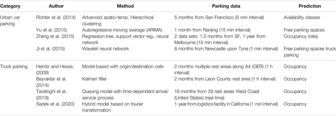
TABLE 1. Summary literature review: Parking prediction.

2.3 Research Gap

Truck parking occupancy prediction research along highways seems to be dominated by domain-knowledge-supported prediction methods as shown in the previous section. The models perform well, but are either limited to a specific environment, need extensive additional data sources (i.e., other than historic occupancy data), or could not be extensively validated. On the other hand, parking prediction work in urban environments tends to use more generic time series clustering and forecasting techniques, which require less domain knowledge but focus on shorter forecasting horizons or work only with availability classes (low, medium, high). This work closes the gap by addressing the shortcomings of today’s truck parking prediction work by leveraging domain-knowledge-light generic forecasting techniques. The objective is to propose a model that requires neither additional data sources (other than historic truck parking occupancy) nor clustering of days with similar trends yet still provides high accuracy. A literature review performed in other traffic domains (i.e., in travel time and traffic flow prediction) suggests that machine-learning models are well suited for time series prediction by accounting for complex non-linearities (Vlahogianni et al., 2004; Lv et al., 2015; Mori et al., 2015; Polson and Sokolov, 2017; Zhao et al., 2017; Zhang et al., 2019; Ting et al., 2020). However, in our literature review, we could not find any extensive work on truck parking prediction based on machine-learning. This is somewhat surprising given the urgency of the truck parking issue. We therefore pursue two objectives:

• Applying XGBoost, which is one of the most promising algorithms in other traffic forecasting domains (Dong et al., 2018; Mei et al., 2018; Ting et al., 2020), and comparing it to classical time series prediction techniques.

• Developing a meta model with improved prediction accuracy by fusing XGBoost with LSTM

By meta model, also known as meta-learner, we mean model stacking (Breiman, 1996). The aim of a meta model is to combine individual base learners to obtain improved performance. We use a feed-forward neural network as meta model. It combines the XGBoost model and the LSTM model, which represent the individual base learners. For more information on stacking and meta-learners, see Zhou (2012). LSTM models are considered suitable for time series prediction in general (Gers et al., 1999) and, in addition to XGBoost, also show good performance in other traffic domains (Altché and de La Fortelle, 2017; Zhao et al., 2017; Park et al., 2018). By developing a robust and accurate meta prediction model, the many research initiatives concerning automatic truck counting technology (Garber et al., 2004; Haghani et al., 2013; Sun et al., 2018) for real time information could easily provide reliable prediction information with our data-economic approach. Automatic truck counting technology is the basis of Intelligent Truck Parking (ITP), which “is concerned with the management of information related to Truck Parking Area (TPA) operations for HGV” (Sochor and Mbiydzenyuy, 2013). The benefits of ITP, according to Bayraktar et al. (2014), are increased operational efficiency of the drivers, reduced parking on shoulders, reduced fatigue-related crashes, and the reduction of diesel emissions.

In general, patterns exist in parking (Richter et al., 2014; Ji et al., 2015; Tavafoghi et al., 2019; Sadek et al., 2020), but these must be linked to the current occupancy to obtain accurate forecasts. We extract parking patterns from the data and always compare our models to these patterns. This approach allows us to show the performance gains that can be achieved by taking current occupancy into account.

3 XGBOOST and Long Short-Term Memory Model Fusion

This section describes the mathematical foundations of Extreme Gradient Boosting and Long Short-Term Memory. We then connect both estimators with the help of a neural feed-forward network in order to obtain a meta-model capable of reliable multi-step occupancy predictions.

3.1 Extreme Gradient Boosting

XGBoost is a powerful ensemble learning technique that achieves state-of-the-art results in various machine learning competitions (Chen and Guestrin, 2016). Ensemble learning techniques combine several weak (er) base learners to obtain a strong learner (i.e., model). Boosting refers to training the base learners in a sequential manner by reducing the error made by the previous combination of base learners (Friedman, 2002). In the following, the XGBoost is explained according to Chen and Guestrin (2016) with second order Taylor expansion for approximation of the loss function (Friedman et al., 2000).

Let $X\in {\mathrm{ℝ}}^{n\times m}$ be the feature matrix and $\mathit{y}\in {\mathrm{ℝ}}^n$ the target vector, each with n training samples. $\left\{{\mathit{x}}_i\in {\mathrm{ℝ}}^m,y_i\in \mathrm{ℝ}\right\}$ denotes a single training instance. Let the base learners be regression trees and the function space be $\mathrm{ℱ}=\{f\left(\mathit{x}\right)={\mathit{w}}_{q\left(\mathit{x}\right)}\}$, where $\mathit{w}\in {\mathrm{ℝ}}^T$ is the vector of leaf weights. There are T leaves, and $w_j$ denotes the jth leaf score. Each tree is represented by $q:{\mathrm{ℝ}}^m\to \left\{\mathrm{1,2},\dots ,T\right\}$ that maps ${\mathit{x}}_i$ to the corresponding leaf score $w_{q\left(\mathit{x}\right)=j}$. The model output thus consists of K combined base learners:

${\widehat{y}}_i=\stackrel{K}{{\displaystyle \sum }_{k=1}}{f}_k\left({\mathit{x}}_i\right)\text{with}{f}_k\in \mathrm{ℱ}(1)$

Let t be the prediction iteration variable. ${\widehat{y}}_i^t$ then denotes the prediction at the tth iteration for the ith training instance. The regularized loss function for the tth iteration is given by:

${\mathrm{ℒ}}^t=\stackrel{n}{{\displaystyle \sum }_{i=1}}l\left(y_i,{\widehat{y}}_i^{t-1}+f_t\left({\mathit{x}}_i\right)\right)+\text{Ω}\left(f_t\right)(2)$

$\text{Ω}\left(f\right)=\gamma T+0.5\lambda {\Vert \mathit{w}\Vert }^2$

The loss function of predicted values and target values is $l(\cdot ,\cdot )$. $\text{Ω}\left(f\right)$ denotes the regularization term, the parameter γ denotes the minimum loss required for further splitting, and the parameter λ denotes the classical regularization term concerning the leaf scores. The prediction ${\widehat{y}}_i$ is improved by the tth additive function $f_t\left({\mathit{x}}_i\right)$. The objective at this stage is to find the $f_t$ that minimizes the overall loss function ${\mathrm{ℒ}}^{\left(t\right)}$. In order to be applicable for a general loss function, approximation with second order Taylor expansion can be used.

${\widetilde{\mathrm{ℒ}}}^t\approx \stackrel{n}{{\displaystyle \sum }_{i=1}}[l\left(y_i,{\widehat{y}}_i^{t-1}\right)+{\partial }_{{\widehat{y}i}^{\left(t-1\right)}}l\left(y_i,{\widehat{y}}_i^{t-1}\right)f_t\left({\mathit{x}}_i\right)+\frac{1}{2}{\partial }_{{\widehat{y}i}^{\left(t-1\right)}}^{2}l\left(y_i,{\widehat{y}}_i^{t-1}\right)f_t^2\left({\mathit{x}}_i\right)]+\text{Ω}\left(f_t\right)(3)$

The approximated loss function can be simplified by removing constant terms. Furthermore, all training instances belonging to leaf j can be written as belonging to the set $I_j=\left\{i\right|q\left({\mathit{x}}_i\right)=j\}$. The first and second order derivatives can be subsumed as $g_i={\partial }_{{\widehat{y}i}^{\left(t-1\right)}}l\left(y_i,{\widehat{y}}_i^{t-1}\right)$ and $h_i={\partial }_{{\widehat{y}i}^{\left(t-1\right)}}^{2}l\left(y_i,{\widehat{y}}_i^{t-1}\right)$. Additionally expanding the regularization term $\text{Ω}\left(f_t\right)$ leads to:

$\begin{array}{c}{\widetilde{\mathrm{ℒ}}}^t=\stackrel{n}{{\displaystyle \sum }_{i=1}}[g_i{f}_t\left({\mathit{x}}_i\right)+\frac{1}{2}{h}_i{f}_t^2\left({\mathit{x}}_i\right)]+\gamma T+0.5\lambda \stackrel{T}{{\displaystyle \sum }_{j=1}}{w}_j^2\\ =\stackrel{T}{{\displaystyle \sum }_{j=1}}[\left({\displaystyle \sum }_{i\in I_j}{g}_i\right)w_j+0.5w_j^2\left({\displaystyle \sum }_{i\in I_j}{h}_i+\lambda \right)]+\gamma T\left(4\right)\end{array}$

For a given tree structure $q\left(\mathit{x}\right)$, the optimal weight for leaf j is computed as follows:

$\frac{\partial {\widetilde{\mathrm{ℒ}}}^t}{\partial w_j}=0w_j^{\text{∗}}=-\frac{{{\displaystyle \sum }}_{i\in I_j}{g}_i}{{{\displaystyle \sum }}_{i\in I_j}{h}_i+\lambda }(5)$

The optimal value $w_j^{\text{*}}$ can be substituted in Eq. 4 in order to obtain metrics for the respective tree structure. Eq. 6 describes how good or bad the tree is in being able to reduce the loss function.

${\widetilde{\mathrm{ℒ}}}^t\left(q\right)=-0.5\stackrel{T}{{\displaystyle \sum }_{j=1}}\frac{{\left({{\displaystyle \sum }}_{i\in I_j}{g}_i\right)}^2}{{{\displaystyle \sum }}_{i\in I_j}{h}_i+\lambda }+\gamma T(6)$

The loss function depends on a particular tree structure q. Different tree structures can be checked either by trying out all possible structures, which might be infeasible for large data sets, or by using intelligently picked split points.

3.2 Long Short-Term Memory

LSTM networks were proposed by Hochreiter and Schmidhuber (1997) and have been further improved since then. LSTMs are recurrent neural networks that are well suited to handle sequence data for which past timesteps and the context matter for the next timestep. One of the main advantages of LSTMs compared with ordinary recurrent networks is the ability to better handle the exploding and vanishing gradient problem (Hochreiter and Schmidhuber, 1997; Pascanu et al., 2013). An LSTM Network consists of LSTM blocks, which have input i, forget f, and output o gates. The output of the previous block is recurrently fed into the next block as block input z and, together with the three gates, updates the cell state. LSTM may exist with or without peephole connections, which allow the gates to get information from the cell state (Gers et al., 2003). In the following, a forward pass with peephole connections is described according to Greff et al. (2017) with a few notional changes.

Let $\mathit{x}=\left({\mathit{x}}^0,{\mathit{x}}^1,\cdots ,{\mathit{x}}^T\right)$ have T timesteps with ${\mathit{x}}^t\in {\mathrm{ℝ}}^m$ being the input vector at timestep t. The number of LSTM memory cells is denoted by N. Let $\sigma \left(\mathit{x}\right)$ be the point-wise applied logistic sigmoid and $g\left(\mathit{x}\right)=h\left(\mathit{x}\right)$ be the point-wise applied hyperbolic tangent. The Hadamard product is denoted by $\odot$. Let the weights be defined as follows:

$\text{Weight matrices for inputs: }{W}_z,W_i,W_f,W_o\in {\mathrm{ℝ}}^{n\times m}$

$\text{Recurrent weight matrices: }{R}_z,R_i,R_f,R_o\in {\mathrm{ℝ}}^{n\times m}$

$\text{Bias weight vectors: }{\mathit{b}}_z,{\mathit{b}}_i,{\mathit{b}}_f,{\mathit{b}}_o\in {\mathrm{ℝ}}^n$

$\text{Peephole weight vectors: }{\mathit{p}}_i,{\mathit{p}}_f,{\mathit{o}}_o\in {\mathrm{ℝ}}^n$

3.2.1 Forward Propagation

The block input features the input vector ${\mathit{x}}^t$, the previous step output ${\mathit{y}}^{t-1}$, and the respective bias.

${\overline{\mathit{z}}}^t=W_z{\mathit{x}}^t+R_z{\mathit{y}}^{t-1}+{\mathit{b}}_z$

${\mathit{z}}^t=g\left({\overline{\mathit{z}}}^t\right)(7)$

The input and forget gates look similar but also feature respective peephole connections that look at the cell state. The two gates are used to update the cell state. The output gate already looks at the updated cell state through the peephole connection.

$\begin{array}{ll}\hfill & {\overline{\mathit{i}}}^t=W_i{\mathit{x}}^t+R_i{\mathit{y}}^{t-1}+{\mathit{b}}_i+{\mathit{p}}_i\odot {\mathit{c}}^{t-1}\hfill \\ \hfill & {\mathit{i}}^t=\sigma \left({\overline{\mathit{i}}}^t\right)\hfill \\ \hfill & {\overline{\mathit{f}}}^t=W_f{\mathit{x}}^t+R_f{\mathit{y}}^{t-1}+{\mathit{b}}_f+{\mathit{p}}_f\odot {\mathit{c}}^{t-1}\hfill \\ \hfill & {\mathit{f}}^t=\sigma \left({\overline{\mathit{f}}}^t\right)\hfill \end{array}\begin{array}{ll}{\mathit{c}}^t\hfill & ={\mathit{z}}^t\odot {\mathit{i}}^t+{\mathit{c}}^{t-1}\odot {\mathit{f}}^t\hfill \\ {\overline{\mathit{o}}}^t\hfill & =W_o{\mathit{x}}^t+R_o{\mathit{y}}^{t-1}+{\mathit{b}}_o+{\mathit{p}}_o\odot {\mathit{c}}^t\hfill \\ {\mathit{o}}^t\hfill & =\sigma \left({\overline{\mathit{o}}}^t\right)\hfill \end{array}(8)$

Finally, the block output is given by:

${\mathit{y}}^t=h\left({\mathit{c}}^t\right)\odot {\mathit{o}}^t(9)$

After the forward propagation, backpropagation through time is needed to adjust the weights. For the interested reader, this is described in the Supplementary Material under Backpropagation Through Time.

3.3 Model Fusion With Feed-Forward Neural Network

Our model fusion is based on a feed-forward neural network. We take the predicted output of (I) XGBoost and (II) LSTM in combination with a subset of the original features used for training I and II to develop an even stronger meta-model. Model training for both XGBoost and LSTM is performed with mean-square error (MSE) loss function averaging multioutput uniformly. Let ${\widehat{y}}_{ih}$ and $y_{ih}$ be the predicted occupancy and the true occupancy of instance $i\in \left\{1,\dots ,N\right\}$ and forecasting step $h\in \left\{1,\dots ,M\right\}$, respectively. MSE for multioutput is then defined as:

$\begin{array}{l}L\left(\widehat{y},y\right)=\frac{{\Sigma }_{i=1}^N{\Sigma }_{h=1}^M{\left({\widehat{y}}_{ih}-y_{ih}\right)}^2}{M\times N}\\ \\ \end{array}(10)$

The feed-forward neural network is trained with the same loss function. The resulting model is referred to as the Truck Parking Prediction (TPP) model. With this type of model fusion, the feed-forward neural network learns to dynamically weight the predictions of the XGBoost and the LSTM model.

The architecture of the TPP model is shown in Figure 1. On the bottom left, the LSTM model consists of an encoder layer with 30 memory units and a decoder layer with 50 memory units. In both layers, a hyperbolic tangent activation function is used. The two layers are connected by a repeat layer in order to match the three-dimensional input requirements of the decoder layer. The final layer is a time-distributed, densely connected layer with linear activation function, which is typically used for regression tasks. It is not the unrolled version of the LSTM but rather a high level perspective focusing on the number of units (also known as cells) that is shown. The encoder-decoder model follows the sequence-to-sequence architecture: many-to-many. The efficient and widely used adam (adaptive moment estimation) algorithm (Kingma and Ba, 2017) is used for optimization. Details of the model architecture and training parameters such as training epochs and batch size are found using grid search, which is described under LSTM Grid Search Results. The XGBoost model is shown on the bottom right. There are 80 decision trees with a maximum depth of four for boosting the prediction accuracy. Minimum child weight is set to 3.0, minimum loss reduction gamma to 4.0, and L2 lambda regularization to 3.0. The specific values of the parameters mentioned are again derived from an extensive grid search. The mean-square error loss function for multioutput is used for training.

FIGURE 1

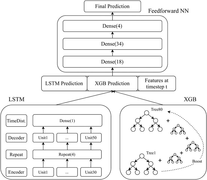
FIGURE 1. Truck parking prediction model.

The predictions of the LSTM and the XGBoost model are combined with time-dependent features before they are used as input in the feed-forward neural network. Let the output at timestep t for the LSTM and the XGBoost model be defined as ${\widehat{y}}_{t+h|t}^{\text{LSTM}}$ and ${\widehat{y}}_{t+h|t}^{\text{XGB}}$ for $h=\left\{\mathrm{1,2,3,4}\right\}$, respectively. Notation-wise, we drop $|t$ in matrix notation for convenience. The following time-dependent features are included.

• $x_t^{\text{occ}}$ : = occupancy of timestep t

• $x_t^{\text{sl}}$ : = occupancy slope (i.e., occupancy change $x_t^{\text{occ}}-x_{t-1}^{\text{occ}}$)

• $x_t^{\text{ban}}$ : = binary variable signaling whether a driving ban is in place at time t

• $x_t^{\diamond \_\text{sin}}$ : = sine encoded time variables, with $\diamond \in \{\text{month},\text{ weekday},\text{ hour}\}$

• $x_t^{\diamond \_\text{cos}}$: = cosine encoded time variables, with $\diamond \in \{\text{month},\text{ weekday},\text{ hour}\}$

The feature input matrix of the feed-forward neural network is defined as follows. N denotes the number of available instances:

$X=\left(\begin{array}{ccccccccccc}{\widehat{y}}_{1,t+1}^{\text{LSTM}}& \dots & {\widehat{y}}_{1,t+4}^{\text{LSTM}}& {\widehat{y}}_{1,t+1}^{\text{XGB}}& \dots & {\widehat{y}}_{1,t+4}^{\text{XGB}}& x_{1,t}^{\diamond \_\text{sin}}& x_{1,t}^{\diamond \_\text{cos}}& x_{1,t}^{\text{sl}}& x_{1,t}^{ban}& x_{1,t}^{\text{occ}}\\ ⋮& & ⋮& ⋮& & ⋮& ⋮& ⋮& ⋮& ⋮& ⋮\\ {\widehat{y}}_{N,t+1}^{\text{LSTM}}& \dots & {\widehat{y}}_{N,t+4}^{\text{LSTM}}& {\widehat{y}}_{N,t+1}^{\text{XGB}}& \dots & {\widehat{y}}_{N,t+4}^{\text{XGB}}& x_{N,t}^{\diamond \_\text{sin}}& x_{N,t}^{\diamond \_\text{cos}}& x_{N,t}^{\text{sl}}& x_{N,t}^{ban}& x_{N,t}^{\text{occ}}\end{array}\right)(11)$

The output for the four prediction steps 30, 60, 90, and 120 min are as follows:

$Y=\left(\begin{array}{ccc}{\widehat{y}}_{1,t+1}^{\text{TPP}}& \dots & {\widehat{y}}_{1,t+4}^{\text{TPP}}\\ ⋮& & ⋮\\ {\widehat{y}}_{N,t+1}^{\text{TPP}}& \dots & {\widehat{y}}_{N,t+4}^{\text{TPP}}\end{array}\right)(12)$

The feed-forward neural network consists of three layers with rectified linear activation functions in the first two layers and a linear activation function in the final layer. No grid search is performed at this stage; this implies that the TPP results could be further improved. In summary, the overall idea of our model fusion is based on model stacking that improves upon the individual base leaners and which is also known as super learner (Breiman, 1996; van der Laan et al., 2007). Stacking is enriched by including additional temporal features.

3.4 Input Data Details

Here, the TPP model structure is defined conceptually. However, the input data for both the LSTM and the XGBoost must be elaborated in order for the model description to be complete. The starting point is a univariate, timestamp-indexed series of occupancy values, which comes from automatic truck counting technology or any other suitable data source. Let $x^{\text{occ}}\left(t\right)=\{x_t^{\text{occ}};t\in T\}$ denote such a time series. First, feature engineering is performed in order to prepare the data to be used in a supervised learning procedure. Temporal features are created from the timestamps by encoding information of the month, weekday, and hour with sine and cosine. For more information regarding temporal feature encoding, see 4.1.5 Feature Engineering. A pattern feature that provides average occupancy values for the corresponding day of the week and time of the day is also included. Finally, an occupancy slope feature and a driving ban feature are added analogously to the explanation in the previous section. The intermediate matrix is as follows:

$A=\left(\begin{array}{cccccccccc}{x}_t^{\text{month}\_\text{sin}}& x_t^{\text{month}\_\text{cos}}& x_t^{\text{weekd}\_\text{sin}}& x_t^{\text{weekd}\_\text{cos}}& x_t^{\text{hour}\_\text{sin}}& x_t^{\text{hour}\_\text{cos}}& x_t^{\text{patt}}& x_t^{\text{sl}}& x_t^{ban}& x_t^{\text{occ}}\\ ⋮& ⋮& ⋮& ⋮& ⋮& ⋮& ⋮& ⋮& ⋮& ⋮\\ x_T^{\text{month}\_\text{sin}}& x_T^{\text{month}\_\text{cos}}& x_T^{\text{weekd}\_\text{sin}}& x_T^{\text{weekd}\_\text{cos}}& x_T^{\text{hour}\_\text{sin}}& x_T^{\text{hour}\_\text{cos}}& x_T^{\text{patt}}& x_T^{\text{sl}}& x_T^{ban}& x_T^{\text{occ}}\end{array}\right)(13)$

Regarding the LSTM model, the intermediate matrix must be transformed into a three dimensional tensor $L_{\alpha ,\beta ,\gamma }$, with α : = number of samples, β: = number of timesteps per sample, and γ : = number of features. The number of samples depends on the data available, $\beta =336$, which corresponds to one week with step size of 30 min, and $\gamma =10$, as can be seen from Eq. 13. For more information on the chosen step size, please refer to Downsampling. Care must be taken that the corresponding output matrix is always ahead of the last input timestep of the respective sample. In the XGBoost model, the intermediate matrix is transformed into a shifted version. The previous 12 timesteps are used as input.

$X^{\text{XGB}}=\left(\begin{array}{cccccc}{x}_{t-11}^{\text{mont}\_\text{sin}}& \cdots & x_{t-11}^{\text{occ}}& x_t^{\text{mont}\_\text{sin}}& \cdots & x_t^{\text{occ}}\\ ⋮& & ⋮& ⋮& & ⋮\\ x_{T-4-11}^{\text{mont}\_\text{sin}}& \cdots & x_{T-4-11}^{\text{occ}}& x_{T-4}^{\text{mont}\_\text{sin}}& \cdots & x_{T-4}^{\text{occ}}\end{array}\right)(14)$

Only values up to $T-4$ can be used in $X^{\text{XGB}}$ because the remaining four values $\left\{x_{T-3}^{\text{occ}},x_{T-2}^{\text{occ}},x_{T-1}^{\text{occ}},x_T^{\text{occ}}\right\}$ are needed for the output matrix. The analogous is true for the LSTM tensor. The number of previous timesteps (336 for LSTM and 12 for XGBoost) provided as inputs performed well in our case study but may have to be adapted for rest areas in other locations.

4 Prediction Pipeline

This section focuses on challenges of missing and incorrect data that come when dealing with real-world truck parking data. Data must be cleaned and preprocessed so that it can be used in machine-learning algorithms. The prediction pipeline is shown in Figure 2.

FIGURE 2

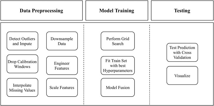
FIGURE 2. Prediction pipeline overview.

4.1 Data Preprocessing

4.1.1 Outlier Handling

Outliers are common for real-world data, and common strategies are to exclude them or to impute them with median values. Outliers first have to be identified (e.g., with bounds based on interquartile ranges). However, for time series data, this is not trivial. First, outliers may be difficult to find. They are not easily detectable in the overall distribution because the time domain must be considered in parallel. Second, outliers cannot simply be dropped because models such as the LSTM need continuous sequence data to learn from unless more sophisticated model structures with masking layers are used. For detecting outliers, we use a Hampel Filter (HF) with window half-width of 30 min and bounds $\pm 3\sigma$. A HF uses a centered sliding window approach and calculates the rolling median and the estimated standard deviation $\sigma =1.4826\times \text{MAD}$ of the window. Let $\left\{x_1^{occ},x_2^{occ},\dots ,x_W^{occ}\right\}$ denote the occupancy values of a univariate time series window with W entries; MAD then denotes the median absolute deviation and is given by: $\text{MAD}=\text{median}\left(|x_1^{occ}-\tilde{x}|,\dots ,|x_W^{occ}-\tilde{x}|\right)$ with $\tilde{x}=\text{median}\left(x_1^{occ},\dots ,x_W^{occ}\right)$. We flag data points lying outside of $\pm 3\sigma$ as outliers and impute them with the median of the respective centered window.

4.1.2 Calibration Handling

Trucks and other vehicles can enter and exit rest areas on the same ramp. Upon entry and exit, each vehicle is classified as a truck or a non-truck by the automatic truck parking detection system (ATPDS). Only if it is classified as a truck, the vehicle is counted with respect to the current occupancy. During the classification process, errors can occur which result in miscounts. The total error increases over time. For this reason, the ATPDS must be calibrated every now and then. To do this, the trucks are recounted manually and compared with the number of trucks counted by the ATPDS. If the deviation before the calibration is large, the occupancy value jumps suddenly during calibration. There are other ATPDSs based on vehicle presence measurements, for example through in-pavement sensors (Sun et al., 2018) or machine vision (Modi et al., 2011). Here, no manual calibration is necessary, and this preprocessing step may be skipped.

First, calibration times must be identified. Times where the occupancy curve rises or drops sharply from subsequent intervals are assumed to be manual calibrations. Our framework uses a threshold value $t_v>|x_t-x_{t-1}|$ for identification. The threshold value depends on the sampling rate of raw data. Our raw data comes in 1 min intervals and we use a hybrid approach of physical plausibility and 99%-quantile to identify the threshold value. We remove 30 min before and after the identified calibration times (calibration removal window) in order to smooth occupancy shocks of manual calibrations.

4.1.3 Missing Values

Missing values can occur in two ways. First, removal of calibration times is accompanied by missing values within the calibration removal window. Second, technical malfunctions may also lead to missing values - possibly also for longer times if the issue is difficult to solve. We propose two approaches to deal with absent values depending on the length of the missing time window. If the missing time window is smaller than a threshold parameter $t_m$, simple linear interpolation can be used. We found that a threshold value of $t_m=3\text{h}$ performs well. However, because of the daily pattern of truck parking occupancy we recommend not exceeding 8 h. This is also supported by the analysis of Bayraktar et al. (2014).

Missing time windows exceeding $t_m$ can not be imputed with linear interpolation because the periodic nature of truck occupancy curves will not be covered. We propose that the average occupancy for the corresponding day of the week and time of the day (weekday pattern curve) be used for filling the missing time window. The data set is therefore grouped by weekday and sampling time interval. The missing time windows are then filled with the respective parts of the weekday pattern curve. This step might introduce occupancy shocks at the transitions from available to imputed data points. However, this issue is alleviated by the following downsampling step.

4.1.4 Downsampling

ATPDSs along a motorway stretch may have different time intervals for updating occupancy values of rest areas that can be harmonized through downsampling. More importantly, machine learning models predict multiples of the intervals they were trained with. In the following, we refer to the interval used in the input data as the step size. In the literature review, forecasting horizons ranging from a few minutes (usually in the urban parking context) to 1 h can be found. Technically, one could use a 1 min step size and forecasting multiples of 1 min. However, the prediction error tends to increase the more forecasting steps are needed. Consequently, predicting 1 h ahead may not be feasible. A downsampling step size of 30 min, which lies in the middle of the values found in literature, is therefore selected. This step size seems to be a good tradeoff between the ability to forecast 1 h or 2 h ahead and the flexibility to frequently incorporate updated occupancy information in the model. Forecasting horizons of up to 2 h, as tested in our study, is our informed guess of what is needed by truck drivers because the distribution when truck drivers start with their search remains a research gap. A study from Chen et al. (2002) merely suggests that 83% of truck drivers decide where to park while they are driving.

4.1.5 Feature Engineering

Important features for time series prediction are temporal components (e.g., month, day, hour). These features are extracted from the timestamps of the ATPDS. However, the features cannot be used in raw form. For example, the raw format for $hour=\left\{1,\dots ,24\right\}$ would attribute 24 times the weight for the last hour of the day compared with the first hour. Moreover, the cyclical nature is not reflected; this means that the model is unable to infer that hour 24 is closer to one than to 20. Let $\diamond$ be element of the set $\left\{\text{month},\text{ weekday},\text{ hour},\text{ minute}\right\}$ and ${\mathit{t}}^{\diamond }$ the vector of the respective time feature (each time feature is assumed to start with 0 not with one e.g., $\text{month}=\left\{0,\dots ,11\right\}$). The cyclical encoding with sine and cosine is thus as follows:

$\begin{array}{c}{x}_i^{\diamond \_cos}=\text{cos}\left(\frac{2\pi t_i^{\diamond }}{\text{max}\left({\mathit{t}}^{\diamond }\right)}\right)\end{array}\begin{array}{c}{x}_i^{\diamond \_sin}=\text{sin}\left(\frac{2\pi t_i^{\diamond }}{\text{max}\left({\mathit{t}}^{\diamond }\right)}\right)\end{array}(15)$

Theoretically, one could provide more features to the model (e.g., traffic volumes, environmental data, and economic data). However, our aim is to develop a widely applicable model that does not depend on difficult to obtain additional data sources. We therefore focus on easily engineered features from raw data. During feature selection, minute-related sine and cosine encoding are found to have no significant effect on model performance and are therefore dropped in order to reduce model complexity.

4.1.6 Feature Scaling

Features can be scaled. Scaling might be needed only for LSTM model training because the tree based XGBoost is invariant of feature scale. The target outputs do not need to be scaled because we deal with a regression task in which a linear activation is used in the final dense layer. In our case study, feature scaling did not have significant positive effects regarding the final meta-model and is therefore not used.

4.2 Model Training and Testing

The preprocessed data set is divided into two equal parts. The first part (training set) is used for optimizing hyper-parameters by cross-validated grid search. Grid search is performed independently for XGBoost and LSTM before the models are fused into the meta-model. In order to thoroughly tune hyper-parameters, cross-validation with 5-fold blocked time series splits is carried out (Figure 3). The data is not shuffled, and each validation set is always ahead of the training set. 5-fold means that the process is performed five times until the end of the hyper parameter tuning set is reached. Blocked time series splits are an improvement over ordinary time series splits in the sense that possible leakage from future timesteps into the model is prevented. The error metric mean-square error is used for scoring. In summary, grid search is performed in order to find the best set of hyper-parameters. By using cross-validation restricted to the first half of the data, we ensure that no knowledge about the hold out test set is leaked into the TPP model. The actual grids tested are explained in Results.

FIGURE 3

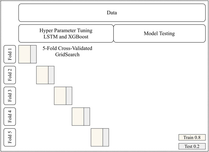
FIGURE 3. Blocked cross-validation.

The hyper-parameters found in grid search are used for training the final XGBoost and LSTM model on the entire training set. Predictions are then made for the test set. These, in turn, serve as features for the feed-forward neural network. Testing of the meta model is conducted using 3-fold cross-validation with blocked time series splits on the test set. A typical train-test split (e.g., 70:30) should not be used at the beginning because only a small portion of data would be available for cross-validation of the TPP model on the test set.

4.2.1 Benchmark Models

We test the TPP model against five different benchmark models. The first two models are based on historical occupancy values and are thus independent of the forecasting horizon. They cannot account for current occupancy levels. The PatternPrevWeek model predicts occupancy based on the previous week’s occupancy on the same day of the week and at the same time of the day. The PatternWeekday model predicts occupancy by calculating the average occupancy for the corresponding day of the week and time of the day from the available training data.

The third is a naive model that predicts the future occupancy value ${\widehat{y}}_{t+h|t}=y_t$. The true occupancy value at time step t is given by $y_t$. Predictions are made for $t+h$ time steps with $h\in \left\{\mathrm{1,2,3,4}\right\}$. For example, $t+1$ represents the point in time 30 min into the future of t because the step size is 30 min. The prediction 30 min ahead is given by ${\widehat{y}}_{t+1|t}$. The expression ${\widehat{y}}_{t+h|t}=y_t$ means that the current occupancy is taken and used as prediction for the four different forecasting steps. This model serves as upper bound. Any model that considers current occupancy levels and performs worse should not be considered a valid model for the truck parking occupancy prediction problem. The model is referred to as the Simple Benchmark Model.

The fourth model is Holt-Winters Triple Exponential Smoothing. The general idea of Simple Exponential Smoothing is to give newer data relatively more weight and older data relatively less weight (i.e., the weights are exponentially decreasing with time). If Simple Exponential Smoothing is extended to incorporate trend and seasonality, it leads to Holt-Winters Triple Exponential Smoothing. We use the non-state-space implementation of statsmodels (v. 0.11.0) with the trend component set to false and optimized parameter estimation. A detailed explanation of the model workings can be found in Hyndman and Athanasopoulos (2018).

The fifth model is SARIMA model, which stands for Seasonal Auto Regressive Integrated Moving Average. It was developed by Box and Jenkins (Box et al., 2015). The idea is that future timesteps of a time series can be predicted by a regression model that uses its own lag values as independent variables (AR part). The model also incorporates lagged forecast errors and can consider them when predicting future timesteps (MA part). A prerequisite for the model to work is a stationary time series, which may be achieved by differencing. Detailed explanation of the model workings can be found in Hyndman and Athanasopoulos (2018). We use a combination of auto-correlation function (ACF) plots, partial auto-correlation function (PACF) plots, and a grid-search-like approach with pmdarima (v. 1.5.3) in order to find the best values for $p=2$, $d=1$, and $q=0$ as well as for the seasonal counterparts $P=0$, $D=1$, and $Q=2$. The seasonality is restricted to one day (i.e., $m=48$, with step size 30 min) because computational resource demand becomes infeasible for one week (i.e., $m=336$) in our development environment.

4.2.2 XGBoost

As described under Research Gap, our first objective is to apply XGBoost, which is one of the most promising algorithms in other traffic forecasting domains, and to compare it to classical time series prediction techniques. The hypothesis is that the XGBoost model shows superior performance compared with classical time series techniques. This is the first time that classical and machine-learning-based models have been evaluated side by side with respect to the truck parking prediction problem. Furthermore, if the hypothesis holds true, the XGBoost model can serve as a tight upper bound for our newly developed TPP model. The XGBoost model is trained with the best hyper-parameters found during grid search. The model details are described under XGBoost Grid Search Results.

4.2.3 Testing

All models, except the two pattern models and the naive model, are 3-fold cross-validation with blocked time series splits on the test set. The testing of the two pattern models is done by ordinary validation on the test set and works as follows. The PatternPrevWeek model is validated on the entire test set by considering the occupancy levels of the previous week. The PatternWeekday model is “trained” with the entire training set and then applied to the test set. With this approach, the PatternWeekday model has more historical training data available which is crucial for a model based only on historical values. The naive model is also validated with the entire test data set, but no public holidays are excluded. With respect to the Holt-Winters and the SARIMA model, testing within the test set of each fold is carried out as follows: at timestep t predictions $\left\{{\widehat{y}}_{t+1|t},{\widehat{y}}_{t+2|t},{\widehat{y}}_{t+3|t},{\widehat{y}}_{t+4|t}\right\}$ are made and evaluated. The true occupancy value of $x_{t+1}^{\text{occ}}$ is then included by refitting the models, and the subsequent predictions $\left\{{\widehat{y}}_{t+1|\tilde{t}},{\widehat{y}}_{t+2|\tilde{t}},{\widehat{y}}_{t+3|\tilde{t}},{\widehat{y}}_{t+4|\tilde{t}}\right\}$ are evaluated. $\tilde{t}$ denotes t which is shifted forward by 30 min. The procedure is repeated until the end of the test set of the respective fold is reached. With this approach, a fair comparison of all models is guaranteed.

5 Results

5.1 Data Background

We collected occupancy data of a truck parking facility in Bavaria with 1 min resolution over one entire year. The rest area is called Offenbau West, has 50 truck parking spaces (overcrowding occurs frequently), and is situated along the motorway between the two biggest cities in Bavaria: Nuremberg and Munich. The rest area is equipped with a high accuracy truck parking detection system consisting of laser and radar measurements at the entrance and exit of the rest area. From January 1, 2019 12:01 a.m. to December 31, 2019 11:59 p.m. we gathered 499,500 data records, each consisting of a local timestamp and an occupancy value. Only 5% of data records are missing. This is mainly due to technical failures, communication issues, or short interruptions for maintenance. In total, 14 outliers were detected and three calibration times were identified. With respect to calibration detection, we found that a threshold value of 12 trucks works well for us; this is an equivalent of two trucks coming in or going out every 10 s. Missing data, outliers, and calibration times are handled by the PP as described in Data Preprocessing. Figure 4 shows two weeks of training data as an example to explain the general characteristics. The first two lines represent raw data and preprocessed data from March 25, 2019 to April 8, 2019. The analysis of the data shows that truck parking occupancy data exhibits weekday and weekend patterns. Truck drivers depart from the rest area in the morning hours between 4:30 a.m. and 8:00 a.m. and arrive in the evening hours between 4:00 p.m. and 12:30 a.m. during weekdays. During weekdays, between 9:00 a.m. and 3:00 p.m., the occupancy stays relatively stable at a low level. The weekend pattern differs from the weekday pattern; fewer trucks need parking, and only 30–70% of the available capacity is used. Furthermore, less change in occupancy is seen on Sundays because trucks are not allowed to drive in Germany by law unless the driver holds a special permit. In summary, the occupancy patterns are in line with observations from other countries (Sun et al., 2018). The third line in Figure 4 shows the weekday pattern (i.e., the average occupancy for the corresponding day of the week and time of the day). All available data, not just the training data, is used to illustrate the best possible weekday pattern curve. Normally, training and test data sets are kept strictly separate, but in this case an exception is made. Public holidays are excluded to avoid distortions. It can be seen that the occupancy values in the first week fit better than in the second week. In particular in the second week towards the end, the values deviate. In general, the weekday pattern cannot fully capture the dynamics of truck parking. Hence, more complex models are needed to obtain reliable predictions (Sadek et al., 2020). However, predictions based on historical patterns can represent an upper bound as shown in Figure 5.

FIGURE 4

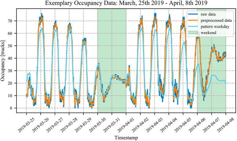
FIGURE 4. Occupancy raw data example.

FIGURE 5

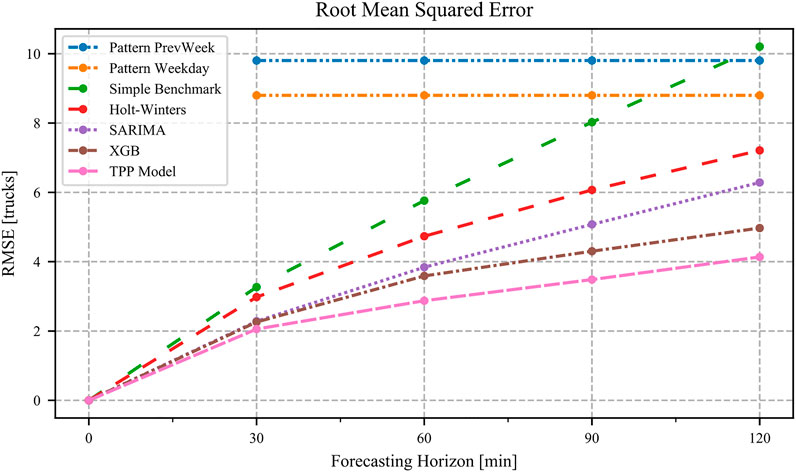
FIGURE 5. Prediction performance.

5.2 XGBoost Grid Search Results

In order to find the best hyper-parameters, grid search is carried out using 5-fold blocked time series split cross-validation on the training set. MSE is calculated for multistep output n = 4 (i.e., forecasts 30, 60, 90, and 120 min). 5,760 hyper-parameter combinations were tested regarding the XGBoost model. For the implementation, we used XGBoost (v. 0.90) with the scikit-learn library, which provides convenient parallel grid search capabilities. The search is performed on Ubuntu 18.04 LTS server with AMD EPYC 7702P 64-Core CPU, 768GB RAM, and Nvidia GeForce RTX 3090 24 GB. The grid consists of:

• Maximum depth of trees: $D_{Trees}=\left\{\mathrm{3,4,5,6}\right\}$

• Minimum child weight: $W_{Child}=\left\{\mathrm{3,3.5},\dots ,6.5\right\}$

• Minimum loss reduction gamma: $\gamma =\left\{\mathrm{0,0.5},\dots ,4.5\right\}$

• L2 regularization lambda: $\lambda =\left\{\mathrm{1,2,3}\right\}$

• Number of gradient boosted trees: $K=\left\{\mathrm{80,100},\dots ,180\right\}$

The best parameter combination found is: $d_{Trees}^{\text{*}}=4$, $w_{Child}^{\text{*}}=3.0$, ${\gamma }^{\text{*}}=4.0$, ${\lambda }^{\text{*}}=3.0$ and $k^{\text{*}}=80$ with $\text{MSE}=20.27$ and standard deviation $s=6.79$. Grid search only took about 1 h because we were able to take advantage of our multicore server, and the XGBoost implementation is generally quite fast (Chen and Guestrin, 2016).

5.3 LSTM Grid Search Results

We used TensorFlow in combination with scikit-learn for the implementation of the LSTM grid search. During the search, 256 hyper-parameter combinations were tested. The grid consisted of:

• Units LSTM encoder layer: $N_{UnitEnLayer}=\left\{\mathrm{20,30,40,50}\right\}$

• Dropout encoder layer: $D_{EnLayer}=\left\{0.0,0.1\right\}$

• Units LSTM decoder layer: $N_{UnitDeLayer}=\left\{\mathrm{20,30,40,50}\right\}$

• Dropout decoder layer: $D_{DeLayer}=\left\{0.0,0.1\right\}$

• Batch size: $B=\left\{\mathrm{4,8}\right\}$

• Epochs: $E=\left\{\mathrm{35,40}\right\}$

The best parameter combination found consists of: $n_{UnitEnLayer}^{\text{*}}=30$, $d_{EnLayer}^{\text{*}}=0.1$, $n_{UnitDeLayer}^{\text{*}}=50$, $d_{DeLayer}^{\text{*}}=0.1$, $b^{\text{*}}=4$ and $e^{\text{*}}=40$ with $\text{MSE}=20.02$ and standard deviation $s=5.61$. At this point, grid search could be extended with more sophisticated methods and with more parameter combinations. However, sufficient computational resources would be needed. Our grid search with 256 hyper-parameter combinations took about 2.5 days. There are mainly two reasons for the exponentially longer grid search time compared with XGBoost. First, LSTM training takes longer than XGBoost training. Second, training is performed on a single GPU compared with the multicore CPU training. Both MSE and standard deviation of the two models are close. However, the training time of the XGBoost model is significantly faster.

5.4 Model Performance Results

5.4.1 Regression Metrics

Four different error metrics are used to evaluate the performance of the models (Botchkarev, 2019): Root-Mean-Square Error (RMSE), Mean-Square Error (MSE), Mean-Absolute Error (MAE) and Median-Absolute Error (MedAE). RMSE and MSE differ only by a square root. RMSE has the advantage of indicating errors in the same units as the target variable, whereas MSE is often used as objective function in the training procedure. We therefore include both metrics. MedAE is included because it is a more robust measure with respect to outliers (Morley et al., 2018). The general definitions are as follows:

$\text{RMSE}\left(y,\widehat{y}\right)=\sqrt{\frac{1}{N}\stackrel{N}{{\displaystyle \sum }_{i=1}}{\left(y_i-{\widehat{y}}_i\right)}^2}(16)$

$\text{MSE}\left(y,\widehat{y}\right)=\frac{1}{N}\stackrel{N}{{\displaystyle \sum }_{i=1}}{\left(y_i-{\widehat{y}}_i\right)}^2$

$\text{MAE}\left(y,\widehat{y}\right)=\frac{1}{N}\stackrel{N}{{\displaystyle \sum }_{i=1}}|y_i-{\widehat{y}}_i|$

$\text{MedAE}\left(y,\widehat{y}\right)=\text{median}\left(\right|y_i-{\widehat{y}}_i\left|\right)\text{for}i\in N$

The error metrics are applied for each forecasting step respectively. The reported values are calculated by averaging the results from cross-validation on the test set. The following explanation of the results is mainly based upon the error metrics RMSE. In Figure 5, the results of the TTP model in comparison with the other models are shown. The figure indicates RMSE for forecasting horizons of 30, 60, 90, and 120 min. An overview of RMSE and MAE is shown in Table 2. All computed model metrics can be found in the Supplementary Material in Supplementary Table S2.

TABLE 2

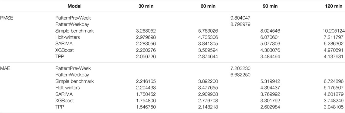
TABLE 2. Model metrics.

The PatternPrevWeek model represents the upper bound with RMSE of about 10 trucks. The PatternWeekday model can improve the prediction by about one truck. The errors refer equally to all “forecasting horizons” because the occupancy is derived from historical values for the corresponding day of the week and time of the day. As expected, the performance of all remaining models decreases with longer forecasting horizons. The Simple Benchmark model shows a nearly linear increase in RMSE that intersects with the pattern models at the end. The Holt-Winters model can improve the prediction quality significantly compared to the Simple Benchmark model, particularly for longer forecasting horizons. Regarding 30 min forecasts, there are only small differences (3.3 vs 3.0 trucks) noticeable, whereas for 120 min forecasts, Holt-Winters can improve by about three trucks. The SARIMA model shows improved performance compared with Holt-Winters and exhibits similar prediction errors compared with the XGBoost model with respect to shorter prediction horizons (2.3 vs 2.2 trucks). However, when the prediction horizons are increased, the XGBoost model clearly outperforms SARIMA. The SARIMA model can achieve RMSE metrics of 6.3 trucks, whereas the XGBoost model reaches 5.0 trucks. To our best knowledge, we are the first to apply XGBoost to the truck parking prediction problem.

With these findings, our first research objective as described under Research Gap is achieved. Our second research objective is to investigate whether predictions of the XGBoost model can be further improved by model fusion. We therefore fused the XGBoost and LSTM model with the help of a feed-forward neural network. The TPP model shows the best performance of all models because it can make the most accurate predictions for all forecast horizons. The RMSE metrics for the four different horizons are 2.1, 2.9, 3.5, and 4.1 trucks, respectively. This means that the predictions of the TPP model are 50% better than those of the PatternWeekday model in terms of 120 min forecasts. However, the performance improvement comes at the cost of increased computational resources for training the model. The average model training times resulting from cross-validation on the test set are depicted in Table 3. No training times are presented for the two pattern models because training is not needed. The calculation of the TPP model consists of two steps because of the more complex, stacked training procedure. First, the training times for XGBoost and LSTM on the training set are measured. Second, these training times are added to the average training times of the TPP model resulting from cross-validation. The results indicate that our TPP model has the highest training times of all models, which is the price of high accuracy predictions. XGBoost has the lowest training times. However, training times in the order of magnitude of under 30 min might not make a big difference in practice. First, it remains to be researched how often retraining of the model is needed. Second, even if retraining is needed on a daily basis, it could be performed during nights, when most truck drivers are asleep. In summary, machine-learning-based models outperform classical time series techniques. In terms of training speed, the XGBoost model outperforms all other models. The proposed TPP model performs best with respect to prediction accuracy.

TABLE 3

TABLE 3. Model training times.

5.4.2 Classification Metrics

In addition to the regression metrics, type I and type II errors are evaluated. All models are set up to predict occupancy values (regression task). Predicting occupancy instead of free parking spaces has advantages when the maximum (legally) allowed capacity is often exceeded. Our investigated rest area has 50 official truck parking spaces. However, Figure 4 shows, as an example, that there are more than 60 trucks regularly parked during working days (also see the pattern curve). This leads to a general discussion about the maximum capacity of a rest area. The main point of this discussion is, how much overcrowding should be tolerated. In addition, the question arises as to whether it is permissible to display the tolerated overcrowding capacity (legal implications). The prediction of remaining free parking spaces means that a maximum capacity threshold must be set. If the official maximum capacity is taken, truck drivers will most likely not trust the prediction. Moreover, the information is lost by how much the official capacity limit is exceeded. We therefore decided to predict occupancy values because this is the most objective way. In order to evaluate type I and II errors, the problem is transformed into a binary classification task. For this, a capacity threshold must be assumed above which the rest area is considered full. The threshold is assumed to be 50 parking spaces according to the official maximum capacity. The predicted occupancy values are transformed by a binary mapper. One means that there are still free parking spaces, whereas zero indicates that the rest area is closed. Table 4 shows type I and II errors for all models and forecasting horizons. The best values are marked in bold. Type I error (false positive) indicates that the model incorrectly predicts free spaces, while the rest area will be full in reality. Type II error (false negative) indicates that the model incorrectly predicts a full rest area, while it will not be full in reality.

TABLE 4

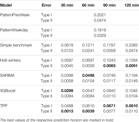
TABLE 4. Type I and type II error. The best values of the respective prediction horizon are marked in bold.

Table 4 shows an increasing trend for type I and II errors for all models (where applicable) as the prediction horizon becomes longer. Type I errors are larger than type II errors for all models. This means that the probability of incorrectly predicting an open rest area is higher than the probability of incorrectly predicting a closed rest area. Type I error is more severe from the truck driver’s point of view. The TPP model is the only model that manages to keep the type I error relatively stable below 7% for longer prediction horizons. However, the XGBoost and the SARIMA model perform better than the TPP model with respect to shorter prediction horizons. In terms of type II errors, the TPP model performs best for shorter prediction horizons, whereas the Holt-Winters model performs slightly better for longer horizons. In conclusion, type I and type II error evaluation shows that predictions based on historical patterns are outperformed by the other models. Regarding the more severe type I error, the TPP model exhibits a more stable behavior with respect to longer prediction horizons than the other models. However, the overall picture is not as clear as when evaluating the regression metrics. The problem was set up as a regression task that accurately predicts occupancy values. Hence, the clear picture when evaluating the regression metrics. Figure 6 shows the binary confusion matrix for the TPP model with respect to the different forecasting horizons. The largest error rate of 1.6% is reported for 120 min forecasts. The confusion matrices of the remaining models can be found in the Supplementary Material.

FIGURE 6

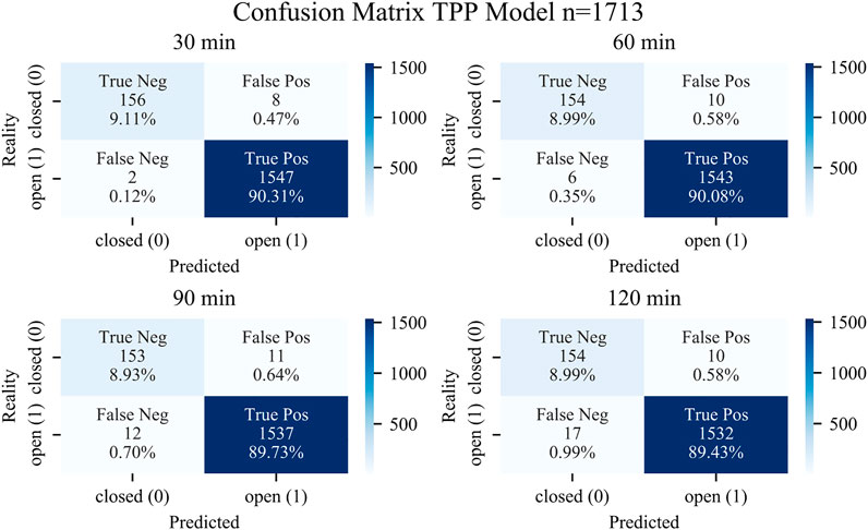
FIGURE 6. Binary confusion matrix TPP model.

6 Conclusion and Discussion

We show that truck parking occupancy prediction is still in its infancy. This is surprising given how pressing the issue of truck parking is. Machine-learning-based prediction models have received little attention from researchers in the field so far, even though they show promising results in other traffic related problems, such as travel time and traffic flow prediction. However, the data availability and resources needed for preprocessing the data determine the success of data-driven machine-learning models. The aim of this study was therefore to develop a prediction model that does not require additional data sources other than historic truck parking occupancy yet still provides high accuracy. Furthermore, the model should be able to deal with real-world data with all its complexities. For our case study, we collected real-world data from a rest area along the motorway A9 in Germany over 1 year. The occupancy data collected consists of a timestamp and occupancy value in 1-min intervals. We show that even for one data source, intensive data preprocessing is necessary, and we systematically describe the steps required to achieve this.

With the preprocessed data available, we applied XGBoost and compared the performance with classical time series prediction techniques Holt-Winters and SARIMA. The results indicate that XGBoost outperforms the benchmark models with respect to both accuracy and training time. We also investigated whether the model fusion of two different machine-learning models can further improve prediction accuracy. We therefore fused the XGBoost and LSTM model with the help of a feed-forward neural network. The resulting TPP meta-model is compared to all other models with respect to various regression error metrics. All error metrics tested indicate that our proposed TPP model outperforms the other forecasting models, including the XGBoost model. The RMSE metrics for the four different horizons 30, 60, 90, and 120 min are 2.1, 2.9, 3.5, and 4.1 trucks, respectively. Predicting whether a free parking space will be available requires assuming a maximum capacity of the rest area. In practice, this is not an easy task because it is a trade-off between the trustworthiness of the prediction and the legal constraints. The prediction of available parking spaces also allows the evaluation of type I and type II errors. With respect to the more severe type I error, the TPP model exhibits a more stable behavior than the other models in terms of longer prediction horizons. However, the overall picture is not as clear as when evaluating the regression metrics. We hypothesize that treating the problem as a classification task instead of a regression task could lead to a further increase in performance. However, other benchmark models would be needed to represent the classification task and to obtain suitable upper bounds. In summary, our TPP model appears to be well suited for predicting the occupancy of rest areas along motorways and could thus partially relieve truck drivers from the stress of searching for a suitable overnight parking space. The unique feature of our proposed model is that only readily available data is used as input. This, in turn, makes it readily applicable in practice. With our work, the many research initiatives concerning automatic truck counting technology for ITP could provide reliable prediction information on top of the current capabilities.

In conclusion, the overall motivation of the study was to improve the truck parking problem. In general, there are two approaches to solving the truck parking issue according to Smith et al (I) increase parking supply (i.e., building more parking spaces): and (II) better match supply and demand. Building more parking spaces is capital-intensive and might sometimes not be feasible. A more cost-effective and practical solution is to better match supply and demand by the use of ITP (Smith et al., 2005). The benefits of ITP include increased driver operational efficiency, reduced parking on shoulders, reduced fatigue-related crashes, and the reduction of diesel emissions (Bayraktar et al., 2014). Prediction information is considered an important feature of ITP (Smith et al., 2005; Bayraktar et al., 2014) because truck drivers need to know whether parking spots will be available at a downstream stop at their expected arrival time. Our TPP model provides accurate occupancy forecasts enabling better-informed parking decisions than with historical pattern curves or traditional time series methods.

One of the biggest questions, however, remains when truck drivers start looking for parking. While the literature suggests that truck drivers decide while they are driving, the distribution would be of great importance so that predictions for the required horizons can be optimized. Another important aspect is second order effects of predictions (i.e., whether and how prediction information changes parking choice), which in turn affects the forecasts. In principle, the problem is known in traffic research. For example, when studying alternative routing information in the case of traffic jams. We hope that machine-learning-based approaches, which can be trained online, will be part of the solution. As a next step, we seek to collect data from other truck parking detection systems in different countries in order to show the generalization of our TPP model. We are also interested in studying type I and type II errors in more detail when the problem is set up as a classification task.

Data Availability Statement

The raw data supporting the conclusion of this article will be made available by the authors, without undue reservation.

Author Contributions

SG, CM, MS, and KB contributed to conception and design of the study. SG and CM contributed to the literature review. SG developed the model fusion and prepared the prediction pipeline. SG, CM, MS, and KB performed the results analyses. SG and CM wrote sections of the manuscript. All authors contributed to the revision of the manuscript and read and approved the submitted version.

Conflict of Interest

The authors declare that the research was conducted in the absence of any commercial or financial relationships that could be construed as a potential conflict of interest.

Acknowledgments

We thank the Bavarian Road Administration for allowing us to collect data from their automatic truck parking detection system. We would also like to thank our foreign language assistants for proofreading our manuscript and pointing out grammar and spelling mistakes. Lastly, we thank all reviewers for their valuable comments that improved the paper to the highest quality. The authors acknowledge the funds received for open access publication by the TUM Open Access Publishing Fund.

Supplementary Material

The Supplementary Material for this article can be found online at: https://www.frontiersin.org/articles/10.3389/ffutr.2021.693708/full#supplementary-material

References

Altché, F., and de La Fortelle, A. (2017). “An Lstm Network for Highway Trajectory Prediction,” in 2017 IEEE 20th International Conference on Intelligent Transportation Systems (ITSC), 353–359. doi:10.1109/ITSC.2017.8317913

CrossRef Full Text | Google Scholar

Bayraktar, M. E., Arif, F., Ozen, H., and Tuxen, G. (2014). Smart Parking-Management System for Commercial Vehicle Parking at Public Rest Areas. J. Transportation Eng. 141, 04014094. doi:10.1061/(ASCE)TE.1943-5436.0000756

CrossRef Full Text | Google Scholar

Boris, C., and Brewster, R. (2018). A Comparative Analysis of Truck Parking Travel Diary Data. Transportation Res. Rec. 2672, 242–248. doi:10.1177/0361198118775869

CrossRef Full Text | Google Scholar

Botchkarev, A. (2019). A New Typology Design of Performance Metrics to Measure Errors in Machine Learning Regression Algorithms. Ijikm. 14, 045–076. doi:10.28945/4184

CrossRef Full Text | Google Scholar

Box, G., Jenkins, G., Reinsel, G., and Ljung, G. (2015). Time Series Analysis: Forecasting and Control. Wiley Series in Probability and Statistics. New Jersey, NJ: Wiley.

Breiman, L. (1996). Stacked Regressions. Mach Learn. 24, 49–64. doi:10.1007/BF00117832

CrossRef Full Text | Google Scholar

Chen, K. J., Pecheux, K. K., Farbry, J., John, , and Fleger, S. A. (2002). Commercial Vehicle Driver Survey: Assessment of Parking Needs and Preferences (Fhwa-rd-01-160). Washington, DC: Federal Highway AdministrationAvailable at: https://rosap.ntl.bts.gov/view/dot/1000 (Accessed October 19, 2020).

Chen, T., and Guestrin, C. (2016). XGBoost: A Scalable Tree Boosting System. In Proceedings of the 22nd ACM SIGKDD International Conference on Knowledge Discovery and Data Mining (New York, NY, USA: Association for Computing Machinery), KDD ‘16, 785–794. doi:10.1145/2939672.2939785

CrossRef Full Text | Google Scholar

Dong, X., Lei, T., Jin, S., and Hou, Z. (2018). “Short-term Traffic Flow Prediction Based on Xgboost,” in 2018 IEEE 7th Data Driven Control and Learning Systems Conference (DDCLS), Enshi, China (IEEE), 854–859. doi:10.1109/DDCLS.2018.8516114

CrossRef Full Text | Google Scholar

Federal Motor Carrier Safety Administration (2011). Hours of Service of Drivers Final Rule. Fed. Regist. 76 (248). Available at: https://www.govinfo.gov/content/pkg/FR-2011-12-27/pdf/2011-32696.pdf (Accessed October 19, 2020).

Google Scholar

Friedman, J., Hastie, T., and Tibshirani, R. (2000). Additive Logistic Regression: a Statistical View of Boosting (With Discussion and a Rejoinder by the Authors). Ann. Statist. 28, 337–407. doi:10.1214/aos/1016218223

CrossRef Full Text | Google Scholar

Friedman, J. H. (2002). Stochastic Gradient Boosting. Comput. Stat. Data Anal. 38, 367–378. doi:10.1016/S0167-9473(01)00065-2

CrossRef Full Text | Google Scholar

Garber, N. J., Teng, H., and Lu, Y. (2004). A Proposed Methodology for Implementing and Evaluating a Truck Parking Information System. Charlottesville: Center for Transportation Studies, University of VirginiaAvailable at: http://citeseerx.ist.psu.edu/viewdoc/download?doi=10.1.1.202.4376&rep=rep1&type=pdf (Accessed October 19, 2020).

Gers, F. A., Schmidhuber, J., and Cummins, F. (1999). Learning to Forget: Continual Prediction with Lstm. IET Conf. Proc. (5), 850–855. doi:10.1049/cp:19991218

CrossRef Full Text | Google Scholar

Gers, F. A., Schraudolph, N. N., and Schmidhuber, J. (2003). Learning Precise Timing with Lstm Recurrent Networks. J. Machine Learn. Res. 3, 115–143. doi:10.1162/153244303768966139

CrossRef Full Text | Google Scholar

Greff, K., Srivastava, R. K., Koutník, J., Steunebrink, B. R., and Schmidhuber, J. (2017). Lstm: A Search Space Odyssey. IEEE Trans. Neural Netw. Learn. Syst. 28, 2222–2232. doi:10.1109/TNNLS.2016.2582924

PubMed Abstract | CrossRef Full Text | Google Scholar

Haghani, A., Farzinfard, S., Hamedi, M., Ahdi, F., and Khandani, M. K. (2013). Automated Low-Cost and Real-Time Truck Parking Information System. Baltimore: Maryland State Highway AdministrationAvailable at: https://rosap.ntl.bts.gov/view/dot/26675 (Accessed October 21, 2020).

Heinitz, F. M., and Hesse, N. (2009). Estimating Time-dependent Demand for Truck Parking Facilities along a Federal Highway. Transportation Res. Rec. 2097, 26–34. doi:10.3141/2097-04

CrossRef Full Text | Google Scholar

Hochreiter, S., and Schmidhuber, J. (1997). Long Short-Term Memory. Neural Comput. 9, 1735–1780. doi:10.1162/neco.1997.9.8.1735

PubMed Abstract | CrossRef Full Text | Google Scholar

Hyndman, R., and Athanasopoulos, G. (2018). Forecasting: Principles and Practice. 2nd edition. Melbourne, Australia: OTexts.

Jensen, A., and Dahl, S. (2009). Truck Drivers Hours-Of-Service Regulations and Occupational Health. Work. 33, 363–368. doi:10.3233/WOR-2009-0884

PubMed Abstract | CrossRef Full Text | Google Scholar

Ji, Y., Tang, D., Blythe, P., Guo, W., and Wang, W. (2015). Short‐term Forecasting of Available Parking Space Using Wavelet Neural Network Model. IET Intell. Transport Syst. 9 (7), 202–209. doi:10.1049/iet-its.2013.0184

CrossRef Full Text | Google Scholar

Kingma, D. P., and Ba, J. (2017). Adam: A Method for Stochastic Optimization. arXiv. Available at: https://arxiv.org/abs/1412.6980.

Google Scholar

Lv, Y., Duan, Y., Kang, W., Li, Z., and Wang, F.-Y. (2014). Traffic Flow Prediction with Big Data: A Deep Learning Approach. IEEE Trans. Intell. Transport. Syst. 16, 1–9. doi:10.1109/TITS.2014.2345663

CrossRef Full Text | Google Scholar

Mahmud, S., Akter, T., and Hernandez, S. (2020). Truck Parking Usage Patterns by Facility Amenity Availability. Transportation Res. Rec. 2674, 749–763. doi:10.1177/0361198120937305

CrossRef Full Text | Google Scholar

Mei, Z., Xiang, F., and Zhen-hui, L. (2018). “Short-term Traffic Flow Prediction Based on Combination Model of Xgboost-Lightgbm,” in 2018 International Conference on Sensor Networks and Signal Processing (SNSP), 322–327. doi:10.1109/SNSP.2018.00069

CrossRef Full Text | Google Scholar

Modi, P., Morellas, V., and Papanikolopoulos, N. P. (2011). Counting Empty Parking Spots at Truck Stops Using Computer Vision. Minneapolis: Center for Transportation Studies - University of MinnesotaAvailable at: https://rosap.ntl.bts.gov/view/dot/29437 (Accessed October 25, 2019).

Mori, U., Mendiburu, A., Álvarez, M., and Lozano, J. A. (2015). A Review of Travel Time Estimation and Forecasting for Advanced Traveller Information Systems. Transportmetrica A: Transport Sci. 11, 119–157. doi:10.1080/23249935.2014.932469

CrossRef Full Text | Google Scholar

Morley, S. K., Brito, T. V., and Welling, D. T. (2018). Measures of Model Performance Based on the Log Accuracy Ratio. Space Weather. 16, 69–88. doi:10.1002/2017sw001669

CrossRef Full Text | Google Scholar

Nevland, E. A., Gingerich, K., and Park, P. Y. (2020). A Data-Driven Systematic Approach for Identifying and Classifying Long-Haul Truck Parking Locations. Transport Policy. 96, 48–59. doi:10.1016/j.tranpol.2020.04.003

CrossRef Full Text | Google Scholar

Park, S. H., Kim, B., Kang, C. M., Chung, C. C., and Choi, J. W. (2018). “Sequence-to-sequence Prediction of Vehicle Trajectory via Lstm Encoder-Decoder Architecture,” in 2018 IEEE Intelligent Vehicles Symposium (IV), 1672–1678. doi:10.1109/IVS.2018.8500658

CrossRef Full Text | Google Scholar

Pascanu, R., Mikolov, T., and Bengio, Y. (2013). “On the Difficulty of Training Recurrent Neural Networks,” in Proceedings of the 30th International Conference on International Conference on Machine Learning - Volume 28 (JMLR.Org). ICML’13, III–1310–III–1318. doi:10.5555/3042817.3043083

CrossRef Full Text | Google Scholar

Pedregosa, F., Varoquaux, G., Gramfort, A., Michel, V., Thirion, B., Grisel, O., et al. (2011). Scikit-learn: Machine Learning in Python. J. Mach. Learn. Res. 12 (85), 2825–2830. Available at: http://jmlr.org/papers/v12/pedregosa11a.html.

Polson, N. G., and Sokolov, V. O. (2017). Deep Learning for Short-Term Traffic Flow Prediction. Transportation Res. C: Emerging Tech. 79, 1–17. doi:10.1016/j.trc.2017.02.024

CrossRef Full Text | Google Scholar

Richter, F., Di Martino, S., and Mattfeld, D. C. (2014). Temporal and Spatial Clustering for a Parking Prediction Service. In 2014IEEE 26th International Conference on Tools with Artificial Intelligence, 278–282. doi:10.1109/ICTAI.2014.49

CrossRef Full Text | Google Scholar

Sadek, B. A., Martin, E. W., and Shaheen, S. A. (2020). Forecasting Truck Parking Using Fourier Transformations. J. Transp. Eng. Part. A: Syst. 146, 05020006. doi:10.1061/jtepbs.0000397

CrossRef Full Text | Google Scholar

Smith, S. B., Baron, W., Gay, K., and Ritter, G. (2005). Intelligent Transportation Systems and Truck Parking. Washington, DC: U.S. Department of Transportation. doi:10.21949/1502959

CrossRef Full Text | Google Scholar

Sochor, J., and Mbiydzenyuy, G. (2013). Assessing the Benefits of Intelligent Truck Parking. Int. J. ITS Res. 11, 43–53. doi:10.1007/s13177-012-0055-3

CrossRef Full Text | Google Scholar

Sun, W., Stoop, E., and Washburn, S. S. (2018). Evaluation of Commercial Truck Parking Detection for Rest Areas. Transportation Res. Rec. 2672, 141–151. doi:10.1177/0361198118788185

CrossRef Full Text | Google Scholar

Tavafoghi, H., Poolla, K., and Varaiya, P. (2019). A Queuing Approach to Parking: Modeling, Verification, and Prediction. CoRR abs/. 1908, 11479. Available at: http://arxiv.org/abs/1908.11479.

Google Scholar

Ting, P.-Y., Wada, T., Chiu, Y.-L., Sun, M.-T., Sakai, K., Ku, W.-S., et al. (2020). Freeway Travel Time Prediction Using Deep Hybrid Model - Taking Sun Yat-Sen Freeway as an Example. IEEE Trans. Veh. Technol. 69, 8257–8266. doi:10.1109/TVT.2020.2999358

CrossRef Full Text | Google Scholar

van der Laan, M. J., Polley, E. C., and Hubbard, A. E. (2007). Super Learner. Stat. Appl. Genet. Mol. Biol. 6 (1). doi:10.2202/1544-6115.1309

CrossRef Full Text

Vlahogianni, E. I., Golias, J. C., and Karlaftis, M. G. (2004). Short‐term Traffic Forecasting: Overview of Objectives and Methods. Transport Rev. 24, 533–557. doi:10.1080/0144164042000195072

CrossRef Full Text | Google Scholar

Yu, F., Guo, J., Zhu, X., and Shi, G. (2015). “Real Time Prediction of Unoccupied Parking Space Using Time Series Model,” in 2015 International Conference on Transportation Information and Safety (ICTIS), 370–374. doi:10.1109/ICTIS.2015.7232145

CrossRef Full Text | Google Scholar

Yanxu Zheng, Y., Rajasegarar, S., and Leckie, C. (2015). “Parking Availability Prediction for Sensor-Enabled Car parks in Smart Cities,” in 2015 IEEE Tenth International Conference on Intelligent Sensors, Sensor Networks and Information Processing (ISSNIP), 1–6. doi:10.1109/ISSNIP.2015.7106902

CrossRef Full Text | Google Scholar

Zhang, Z., Li, M., Lin, X., Wang, Y., and He, F. (2019). Multistep Speed Prediction on Traffic Networks: A Deep Learning Approach Considering Spatio-Temporal Dependencies. Transportation Res. Part C: Emerging Tech. 105, 297–322. doi:10.1016/j.trc.2019.05.039

CrossRef Full Text | Google Scholar

Zhao, Z., Chen, W., Wu, X., Chen, P. C. Y., and Liu, J. (2017). LSTM Network: a Deep Learning Approach for Short‐term Traffic Forecast. IET Intell. Transport Syst. 11 (7), 68–75. doi:10.1049/iet-its.2016.0208

CrossRef Full Text | Google Scholar

Zhou, Z.-H. (2012). Ensemble Methods: Foundations and Algorithms (Tylor and Francis Group). Boca Raton: chap. 4.4 Combining by Learning, 83–86.