Robot-Based Last-Mile Deliveries With Pedestrian Zones

1 Introduction

There are many challenges associated with last-mile delivery, the final step in the retail supply chain. It is estimated that the last mile constitutes about half of all logistics costs for service providers (McKinsey and Company, 2016). Partially, this is due to the number of failed deliveries, which leads to additional delivery attempts and increased costs. In addition, the rapid growth of e-commerce has increased the demand for delivery drivers (Sasso, 2018) and resulted in driver shortages. With the spread of COVID−19, demand for last-mile delivery services has increased even further. Given these factors, many logistics service providers are exploring alternative solutions for last-mile deliveries.

These solutions include, but are not limited to, cargo bikes, self-service parcel lockers, aerial drones, ground based autonomous delivery robots, crowd shipping, and collection-and-delivery points (Boysen et al., 2020; Janjevic et al., 2019). Some of these solutions are easier to implement than the others. For instance, a wide implementation of electric autonomous vehicles would require substantial investments in the road infrastructure to enable traffic management and coordination (Hussain and Zeadally, 2018). For drone-based deliveries, it has been found that drone noise is more annoying to people than noise emission by vehicles (Christian and Cabell, 2017). Furthermore, in the US, the FAA requires an operator to keep a drone within eye shot while operating and prohibits operating more than one drone at a time by one operator (FAA, 2018). In addition, there is a number of privacy concerns regarding drone operations (Rice, 2019).

In contrast to the above options, the deployment of ground robots seems to be an appealing and promising mode of parcel transportation for last-mile deliveries in the near future. Several companies like Starship (2020), Robby (2020), and Marble (2020) have developed their own versions of delivery robots, which are currently evaluated in field tests. It is common that these delivery robots transport exactly one package to a single customer within a pre-specified time window. The robot moves on the sidewalk at pedestrian speed. Equipped with GPS, cameras, and several other detectors, a robot can operate in an autonomous manner with potentially just one person supervising up to a hundred of them (Sulleyman, 2017). In addition, it is estimated that compared to conventional truck-based deliveries, robot-based deliveries can save up to 90% of operational costs when they are used in a two-tier structure where trucks consolidate packages and deliver them to local robot hubs, where robots undertake the last-mile delivery (Bakach et al., 2021). Generally, people are quite welcoming of these robots, and they are even willing to pay more for parcel deliveries if there is an option to choose the time and location of the delivery (USPS, 2018), which can be easily accommodated by robots. In addition, robots are much smaller than traditional gasoline-powered delivery vans, and their carbon footprint is negligible (Figliozzi, 2020).

The utilization of robots has been steadily increasing across the world. Starship robots have covered over 200,000 km in 20 countries and more than 100 cities around the world, completing over 20,000 grocery and package deliveries (IEEE, 2020). In Milton Keynes, United Kingdom, Starship Technologies launched a robot package delivery service. For a monthly $10 fee, a customer can receive a package delivered by robots from a local static hub (BBC, 2018). With the spread of COVID−19, the delivery app “Meituan Dianping” established contactless deliveries of groceries via robots to customers in Beijing, China (Hu, 2020). Most of the limited amount of academic research on robots is focused on a dynamic-hub approach, where a manned delivery vehicle transports robots and releases them at various locations. In this paper, we focus on the second tier of a two-tier delivery system. In particular, we follow a static-hub approach, where robots travel back and forth between a local hub and customers (see examples in Section 2).

Despite all of the advantages, robots also have several disadvantages that may limit their widespread usage. Limited battery capacity, low speeds, and the necessity of driving on sidewalks are among them. Robots use cameras, radars, and further equipment to navigate safely through a city. However, due to the safety concerns, they must slow down or completely stop in presence of objects, such as pedestrians, in close proximity (Wong, 2017). While robots can help to save a significant amount of labor cost, it is not clear how to best operate them in crowded urban areas. Hence, in this paper, we investigate the impact of congested pedestrian areas on the use of robots for last mile deliveries. Unlike related work, which mostly focuses on deterministic travel times, we explore the effect of stochastic travel times caused by pedestrian level of service (LOS) zones on robot-based deliveries. The LOS reflects the intensity of congestion of traffic flows based on measures such as speed and travel time, freedom to maneuver, traffic interruptions, comfort and convenience (Burden, 2006).

In particular, we investigate the impact of pedestrian LOS zones on an objective known from stochastic vehicle routing as presented by Taş et al. (2013) that reflects customer service quality based on early and late arrivals with known delivery time windows. We assume that the location of the robot hub is given, and all packages and robots are already stored within the robot hub. Robots make multiple pendulum-type trips per day to deliver packages to customers located in different pedestrian LOS zones. These zones reflect different pedestrian intensities and hence affect travel time distributions of robot travel time and the path chosen to the customer. For instance, if there is a pedestrian LOS zone with high pedestrian intensity between a hub and a customer, it might be beneficial for the robot to take a detour to limit exposure to that zone.

This paper provides the following contributions

1) Based on the objective of Taş et al. (2013), we develop a mathematical model for the robot-based last-mile routing problem (RBLMRP) with stochastic travel times and pedestrian LOS zones. We maximize customer service quality, which is a metric based on early and late arrivals.

2) Based on established LOS classifications, we model distributions of robot travel times in urban areas.

3) We adapt path finding and routing heuristics to consider the impact of pedestrian LOS zones on robot traffic.

4) For different pedestrian intensities in LOS zones, we investigate their effect on chosen paths, route plans and customer service quality. This involves the selection from multiple paths between hub and customer, which we call path flexibility. We show that path flexibility is crucial for LOS zones with high pedestrian intensity.

5) We show that extended customer time windows can improve customer service quality by up to 40%.

We provide an overview of related literature in Section 2. In Section 3, we define our problem and present a mixed integer formulation, along with a discussion of issues related to stochastic travel times and objective function evaluation. In Section 4, we present our solution approach. In Section 5, we describe our data sets and computational results. Finally, in Section 6, we provide conclusions and discuss directions for future research.

2 Literature Review

In recent years, the amount of research on new technologies for last-mile deliveries has been growing fast. Emerging concepts are discussed by Speranza (2018), Behnke (2019), Hu et al. (2019) and Boysen et al. (2020). We discuss literature related to robot-based deliveries below. The stochastic nature of travel times in our problem is also related to the stochastic vehicle routing problem with time windows. Thus, we review some of the relevant literature in this field as well.

2.1 Robot-Based Deliveries

Given the large number of publications for last-mile deliveries, the amount of literature on autonomous robot-based deliveries is still quite limited. All existing literature assumes that robots undertake short last-mile deliveries and can be classified into using a dynamic hub or a static hub. With dynamic hubs, robots are released from a mobile hub, such as a delivery truck, but with static hubs, they are released from a local depot.

Dynamic hub concept. Boysen et al. (2018) investigate a problem that consists of one truck, a set of robots, several depots, and a number of drop-off points. The authors consider deterministic travel times with hard customer time windows. In their problem, a truck loaded with parcels and robots moves between drop-off points, where robots are released to conduct last-mile deliveries and then travel to local depots. If the truck runs out of robots, it visits the nearest local depot to pick them up again. Each customer has a delivery deadline. To minimize the number of late deliveries, they combine a multi-start local search heuristic and a mixed-integer program. In results considering up to 40 customers, the model with robots and decentralized drop-off points yields a lower average lateness than an alternative where trucks wait for robots. Ostermeier et al. (2021) consider a combination of a truck, robots, and robot depots, as well as two types of drop-off locations: drop-off points, where a truck releases robots, and robot depots, where it is possible to either release robots from a truck or pick up a robot. Once a delivery has been completed, robots return to a robot depot. A key difference from Boysen et al. (2018) is that in the latter, the robot fleet is more limited. The objective is to minimize combined costs of travel time and distance for the truck and robots along with service costs related to late deliveries. The authors indicate that their approach can reduce costs by up to two thirds compared to the classic truck delivery model. Jennings and Figliozzi (2019) propose a different system: a truck drops off robots for the last mile and instead of continuing its operations, the truck waits for robots to return. The authors apply continuous approximation to estimate the savings that robots can achieve in terms of delivery time and to estimate the number of robots required. They conclude that robots may be more efficient than conventional delivery approaches when the average delivery time per customer is high or when the customer density increases. Simoni et al. (2020) consider a traveling salesman problem with robots and deterministic travel times. One key difference is that the robots have several compartments and can serve multiple customers after leaving a truck. The objective function is to minimize operational costs. The authors develop a dynamic programming approach which can solve instances with up to 100 customers.

Static hub concept. In this paper, we implement a variant of the static hub concept. Poeting et al. (2019) consider a combination of truck routing and static hubs for robot deliveries. In their approach, only a small percent (0–3%) of parcels is delivered by robots directly from robot hubs, which house only one robot. The majority of parcels are delivered by a truck, and the authors focus on the creation of a tour such that customer time windows and hub opening hours are met. Numerical results indicate that such small levels of robot usage have almost no effect on the vehicle tour length. The authors use deterministic travel times with hard customer time windows.

A model developed by Bakach et al. (2021) explores the cost effectiveness of robot-based deliveries compared to conventional truck-based deliveries. A two-tier delivery model is proposed. In the first tier, a truck delivers parcels from a big depot to small local robot hubs, in which a predefined number of robots is maintained. In the second tier, robots make pendulum tours to deliver parcels to customers with and without time windows. The authors propose a mixed integer program to define the minimum number and locations of local hubs and use deterministic travel times with hard customer time windows. In the next step, robots are assigned to customers such that the total travel cost is minimized. The results show that cost is reduced up to 90% compared to conventional delivery methods, mainly due to savings of labor cost. Sonneberg et al. (2019) consider a location-routing problem that utilizes robots to service customers with time windows. Given the multi-compartment nature of the robots, contrasting the layout of current robots promoted by Starship and other companies as used in this paper, several customers can be served by the same robot which drastically decreases the total distance traveled and the number of robots required as compared to the scenario when a robot carries only one parcel. The authors propose a mixed integer program which is used to solve a small case with 10 customers. Similar to the other papers, the authors use deterministic travel times with hard customer time windows.

Ideas considered in this paper differ significantly from the existing literature. First, none of the papers above consider stochastic travel times for robots. Second, all geographies considered in the existing robot literature are homogeneous, so robots move at a predefined speed and follow predefined paths, while we consider path flexibility. To the best of our knowledge, this paper is the first one that addresses these two points.

2.2 Vehicle Routing Problem and Traffic Congestion

There is a large body of research on the vehicle routing problem with stochastic travel times, which is related to our problem, since travel times of robots are stochastic due to varying presence of obstacles. We refer the reader to Rajabi-Bahaabadi et al. (2019) for an overview of existing research on conventional stochastic vehicle routing problems. Among other approaches, stochastic travel times have been modeled with Gamma distributions (Russell and Urban, 2008; Ehmke et al., 2015), and they are important for accurate congestion modeling.

In recent years, modeling of congestion in vehicle routing problems has been an important topic. Contrasting our approach, the most common approach to modeling congestion is via time-dependent travel times that are deterministic (Kok et al., 2012; Ehmke et al., 2012). Related to the zone idea of this paper, Zhang et al. (2019) demonstrate that congestion zones have significant impact on vehicle path selection and that there is a clear benefit in considering congestion zones in routing. However, they also follow a deterministic approach.

To model traffic congestion in zones, traffic engineers describe the utilization of traffic infrastructure using a level of service (LOS) concept. Burden (2006) analyzes the intensity of pedestrian traffic based on pedestrian flow rate and sidewalk space, using categories from LOS “A” indicating free flow and low intensity of pedestrian traffic to LOS “E” indicating severe congestion and high intensity of pedestrian traffic. This approach offers a straightforward way to distinguish between different scenarios of pedestrian traffic intensity. We will use this concept to define different travel time distributions for robot path selection.

Taş et al. (2013) consider a VRP with stochastic travel times and soft customer time windows. They develop a model using Gamma-distributed travel times and propose a solution procedure based on a tabu search algorithm. In our paper, we adopt and modify their objective function as well as their solution approach. We create a heuristic for flexible path selection that considers pedestrian LOS across two zones. In addition, we implement a shifting procedure to allow robots to wait in the robot hub in between parcel deliveries.

3 Problem Definition and Model Formulation

In the following, we define the RBLMRP and present a mathematical model incorporating stochastic travel times. We describe how customer arrival times are modeled and how Gamma distributions are used to reflect different pedestrian intensities in LOS zones.

3.1 Problem Definition

In the RBLMRP, we assume that robots operate from a local hub that contains all robots and packages to be delivered to customers over a certain time period, such as a day. We also assume that the robot hub has the technology to put the right package into each robot. Given this technology and the potential challenges to find locations for such hubs, we assume the hub is static, and the location is given. The objective is to maximize the customer service quality associated with package deliveries based on the expected early and late arrivals. This objective does not include routing cost, since this is negligible in the context of automated operations (Bakach et al., 2021).

Let C = (1, … , m) be the set of potential customers and R = (1, … , n) be the set of robots. Each customer is located within a particular pedestrian LOS zone. Each customer has an associated service time s > 0 and time window (l_c, u_c), l_c ≥ 0, u_c ≥ 0. If a robot arrives to a customer prior to the early time window or after the late time window, a penalty is incurred. A route here is a sequence of trips (robot hub–customer–robot hub) performed by a robot using sidewalks. Since the number of robots coincides with the number of created routes, we use the two terms interchangeably. Each pendulum tour consists of two arcs (robot hub–customer, customer–robot hub), and the arcs have a distance d_c associated with them. For simplicity, we assume that the battery of a robot is replaced after every pendulum tour. We assume that robots are limited to one package per delivery, and each customer receives only one package.

The RBLMRP is modeled mathematically in Section 3.2. The varying intensity of pedestrian traffic as reflected through LOS zones is modelled with Gamma-distributed travel times. These are described in detail in Section 3.3. Since robots may travel across multiple zones to make customer deliveries, travel times may involve combinations of Gamma distributions. This is described in detail in Section 3.4.

3.2 Model Formulation

We formulate the mathematical model of the problem as follows:

$x_c^r=\left\{\begin{array}{cc}1\hfill & :\text{if\hspace{0.17em}robot}r=1,\dots ,n\text{serves\hspace{0.17em}customer}c\text{where}c\in C\hfill \\ 0\hfill & :\text{otherwise}\hfill \end{array}\right.$

$z_{cj}^r=\left\{\begin{array}{cc}1\hfill & :\text{if\hspace{0.17em}customer}j\text{\hspace{0.17em}\hspace{0.17em}immediately\hspace{0.17em}follows\hspace{0.17em}customer}c\text{for\hspace{0.17em}robot}r=1,\dots ,n;\text{where}c,j\in C,c\ne j\hfill \\ 0\hfill & :\text{otherwise}\hfill \end{array}\right.$

$y_c^r=\left\{\begin{array}{cc}1\hfill & :\text{if\hspace{0.17em}customer}c\text{is\hspace{0.17em}first\hspace{0.17em}for\hspace{0.17em}robot}r=1,\dots ,n;\text{where}c\in C\hfill \\ 0\hfill & :\text{otherwise}\hfill \end{array}\right.$

$\mathit{min}\sum _{r=1}^n\sum _{c\in C}{D}_c^r\left(X\right)+\sum _{r=1}^n\sum _{c\in C}{E}_c^r\left(X\right)(1)$

Subject to:

$\sum _{r=1}^n{x}_c^r=1\text{for}c\in C(2)$

$\sum _{j\in C}{y}_j^r\le 1\text{for}r=1,\dots ,n(3)$

$\sum _{c\in C,c\ne j}{z}_{cj}^r+y_j^r=x_j^r\text{for}r=1,\dots ,n;j\in C(4)$

$x_c^r\in \left\{\mathrm{0,1}\right\}\text{for}r=1,\dots ,n;c\in C(5)$

$y_c^r\in \left\{\mathrm{0,1}\right\}\text{for}r=1,\dots ,n;c\in C(6)$

$z_{cj}^r\in \left\{\mathrm{0,1}\right\}\text{for}r=1,\dots ,n;c,j\in C,c\ne j(7)$

Following the objective as presented by Taş et al. (2013), the objective function Eq. 1 minimizes two components associated with the customer service quality of robot deliveries: $E_c^r(x)$ and $D_c^r(x)$. These components represent expected earliness and expected delay at customer c served by robot r. The corresponding costs can be interpreted as costs of customer dissatisfaction that occur when delivering outside the service time window. A detailed formalization of these components is provided in Section 3.3. Constraints Eqs 2–4 ensure that all customers are served by a robot in a particular sequence. Note that Constraints Eq. 3 also allow for some robots to remain at the hub and not be used. Constraints Eqs 5–7 define the domain of the variables.

Despite the simplicity of the model formulation, several challenges arise. First, the evaluation of the objective function requires multiple steps. For every customer, we must determine what path a robot is going to take, and this path determination in the context with different pedestrian LOS zones is a non-trivial problem itself. Path flexibility is important since different paths affect the value of the objective function. Second, the consideration of stochastic travel times adds an additional layer of complexity to the ordering of the customers.

3.3 Modeling Stochastic Travel Times

In our approach, we impose Gamma distributions on the travel times between hubs and customer locations. For the sake of clarity, let us consider the modeling of stochastic travel times for a given route r as follows. We assume that the random time needed to travel one unit of distance on an arc T is Gamma-distributed with shape parameter α and scale parameter λ. In the following, we only vary the shape parameter α and fix the scale parameter λ. This allows us to combine different Gamma distributions for paths in different zones. To this end, suppose T_c is the time needed to travel to customer c from the hub. Since α and λ are parameters associated with T, T_c is Gamma-distributed with parameters α_cd_c and λ obtained by scaling T with respect to the distance d_c between customer c and hub. The mean and variance of T_c are calculated as follows:

$E\left[T_c\right]={\alpha }_c\lambda d_c(8)$

$\mathit{Var}\left(T_c\right)={\alpha }_c{\lambda }^2{d}_c(9)$

By considering travel times with corresponding mean Eq. 8 and variance Eq. 9, we can obtain the expected arrival times Y_c for every customer c. Adapting the approach of Taş et al. (2013), when arriving at a given customer c, the robot has already serviced prior customers in the route, represented through set A_c with customers 1 to c−1, and has returned to the robot hub. The mean and variance of arrival time Y_c depends on the previous travel and arrival times and can be derived as follows for a given customer c:

$E\left[Y_1\right]=E\left[T_1\right](10)$

$Var\left(Y_1\right)=Var\left(T_1\right)(11)$

$E\left[Y_2\right]=E\left[Y_1\right]+E\left[T_1\right]+E\left[T_2\right](12)$

$Var\left(Y_2\right)=Var\left(Y_1\right)+Var\left(T_1\right)+Var\left(T_2\right)(13)$

$\begin{array}{l}\hfill \dots \\ \hfill E\left[Y_c\right]=E\left[Y_{c-1}\right]+E\left[T_{c-1}\right]+E\left[T_c\right]\end{array}(14)$

$Var\left(Y_c\right)=Var\left(Y_{c-1}\right)+Var\left(T_{c-1}\right)+Var\left(T_c\right)(15)$

where Eqs 10, 11 are mean and variance of the arrival time to the first customer on the route, Eqs 12, 13 are mean and variance of the arrival time to a second customer, and Eqs 14, 15 are mean and variance for arrival at customer c−1 which reflects the recursion. Now, Gamma-distributed arrival times Y_c have the following shape (α) and scale (λ) parameters:

${\alpha }_c=2\sum _{l\in A_c}{\alpha }_l{d}_l+{\alpha }_c{d}_c(16)$

${\lambda }_c=\lambda .(17)$

In the form of Taş et al. (2013), the expected delay and expected earliness at customer c in a route can be computed as:

$D_c\left(X\right)={\alpha }_c{\lambda }_c\left(1-{\mathrm{\Gamma }}_{{\alpha }_c+1,{\lambda }_c}\left(l_c\right)\right)-l_c\left(1-{\mathrm{\Gamma }}_{{\alpha }_c,{\lambda }_c}\left(l_c\right)\right)(18)$

$E_c\left(X\right)=e_c{\mathrm{\Gamma }}_{{\alpha }_c,{\lambda }_c}\left(e_c\right)-{\alpha }_c{\lambda }_{rc}{\mathrm{\Gamma }}_{{\alpha }_c+1,{\lambda }_c}\left(e_c\right)(19)$

where α_c and λ_c are parameters that depend on the zone the robot travels through and e_c and l_c are early and late time windows for the customer c. We also adopt the approach from Taş et al. (2013) to service time; we shift the customer time windows to the left by the amount of cumulative service time.

3.4 Combining Travel Time Distributions

When a robot travels from the hub to a customer location, it may be possible that hub and customer are located in different zones characterized by different pedestrian LOS and thus follow Gamma distributions with different parameters. In this case, the path the robot travels consists of two parts, and it needs to be defined how the different parameters of the Gamma distributions are combined to derive expected travel and arrival times at customers.

More formally, assume there are two non-overlapping pedestrian LOS zones (z₁, z₂), and robot r travels a distance of $d_{z_1}$ in Zone 1 and a distance of $d_{z_2}$ in Zone 2 to reach the customer c. Similar to the previous section, we assume that the travel times $T^{z_1}$ in Zone 1 and $T^{z_2}$ in Zone 2 are proportional to the unit of distances traveled in z₁ and z₂, respectively. Furthermore, these travel times are Gamma-distributed with shape parameter ${\alpha }_{z_1}$ and ${\alpha }_{z_2}$ as well as scale parameter λ. Following the approach outlined in the previous section, we obtain $T_c^{z_1}$ and $T_c^{z_2}$, representing the time needed to cover parts of the arc located in zones z₁ and z₂, Gamma-distributed with parameters (${\alpha }_{z_1}{d}_{z_1}$, λ) and (${\alpha }_{z_2}{d}_{z_2}$, λ).

Using the well-known properties of independent Gamma-distributed random variables, we can combine $T_c^{z_1}$ and $T_c^{z_2}$ in order to create $T_c^z$, which represent Gamma-distributed travel times for the entire path. This works as follows. Assume we have $d_{n_1}$ units of distance to be traveled in Zone z₁ and Zone z₂, respectively. From Eqs 8, 9 we obtain:

$\begin{array}{c}\hfill E\left[T_c^{z_1}\right]={\alpha }_{z_1}\lambda d_{n_1}\\ \hfill E\left[T_c^{z_2}\right]={\alpha }_{z_2}\lambda d_{n_2}\end{array}(20)$

and

$\begin{array}{c}\hfill \mathit{Var}\left[T_c^{z_1}\right]={\alpha }_{z_1}{\lambda }^2{d}_{n_1}\\ \hfill \mathit{Var}\left[T_c^{z_2}\right]={\alpha }_{z_2}{\lambda }^2{d}_{n_2}.\end{array}(21)$

Finally, based on the total distance to be traveled, $d_{n_1}+d_{n_2}$, we can derive $T_c^z$ being Gamma-distributed with shape parameter ${\alpha }_{z_1}{d}_{n_1}+{\alpha }_{z_2}{d}_{n_2}$ and scale parameter λ with

$E\left[T_c^z\right]=\left({\alpha }_{z_1}{d}_{n_1}+{\alpha }_{z_2}{d}_{n_2}\right)\lambda (22)$

$Var\left[T_c^z\right]=\left({\alpha }_{z_1}{d}_{n_1}+{\alpha }_{z_2}{d}_{n_2}\right){\lambda }^2.(23)$

The analogous procedure can be applied for the return trip from the customer to the hub, completing the pendulum tour.

4 Solution Approach

To investigate the impact of different pedestrian LOS zones on the routes for robots, we implement a heuristic involving the use of Tabu Search. Our solution approach requires three steps. First, we determine the minimum expected time path between the robot hub and each customer. We discuss this in Section 4.1. Second, we construct an initial solution and improve it with a Tabu Search algorithm, as described in Section 4.2. We further improve the solution with our shifting procedure described in Section 4.3.

4.1 Selection of Minimum Expected Travel Time Paths

Due to the stochastic nature of travel times, the minimum-distance path may not be the one with the lowest expected travel time. Our heuristic chooses the path to a customer with the lowest expected travel time, since it has the greatest chance of meeting the customer’s early time window. Hence, depending on where the hub and customer are located, we need to investigate up to four path candidates. To demonstrate the selection of minimum expected time paths, let us consider the following example with two zones: P, the “outer zone”, characterized by a pedestrian LOS with low intensity (i.e., not many pedestrians on sidewalks), and Q, the “inner zone”, characterized by a pedestrian LOS with high intensity (i.e. many pedestrians on sidewalks). There are the following three cases.

In the first case, portrayed in Figure 1, customer a is located in P, and the minimum-distance path from the hub to the customer lies entirely in P. In this case, the minimum-distance path is also the minimum expected time path. This path has a length d_a and Gamma distributed travel times T∼Γ(α_Pd_a, λ).

FIGURE 1

FIGURE 1. Case 1: Customer a located in low-intensity Zone P.

In the second case, portrayed in Figure 2, customer b is located in Q. Now, we must consider four path candidates, which are created and evaluated as follows:

1) Step 1: Find the location of four zone entry points for Q to reach b. Assuming a grid based city network, we consider only points that are located directly “north”, “east”, “west” and “south” of the customer location. We call paths that uses the “north” entry point a Type-1 path, the “east” entry point a “Type-2” path, the “west” entry point a “Type-3” path and the “south” entry point a “Type-4” path.

2) Step 2: Obtain the distance and expected travel time from the hub to each entry point and from each entry point to the customer. In more detail, since there are four path candidates, we have eight distances. Distances $d_1^P$ and $d_1^Q$ correspond to P and Q parts of Path 1 in Figure 2. Similarly, $d_i^P,i\in \{2,\dots ,4\}$, and $d_i^Q,i\in \{2,\dots ,4\}$, are distances for the partial paths 2, 3, and 4. Using the approach outlined in Section 3.4, we can combine these partial paths and obtain travel time distributions for each of them: $T_i\sim \mathrm{\Gamma }({\alpha }^P{d}_i^P+{\alpha }^Q{d}_i^Q,\lambda ),i\in \{1,\dots ,4\}$. Note that the values α^P and α^Q depend on zone-specific pedestrian LOS.

3) Step 3: Using Eq. 22, we obtain expected travel times for each of the four paths: $E[T_i]=({\alpha }^P{d}_i^P+{\alpha }^Q{d}_i^Q)\lambda ,i\in \{1,\dots ,4\}$.

4) Step 4: Select the path with the minimum expected travel time min E (T_i), i ∈ (1, … , 4).

FIGURE 2

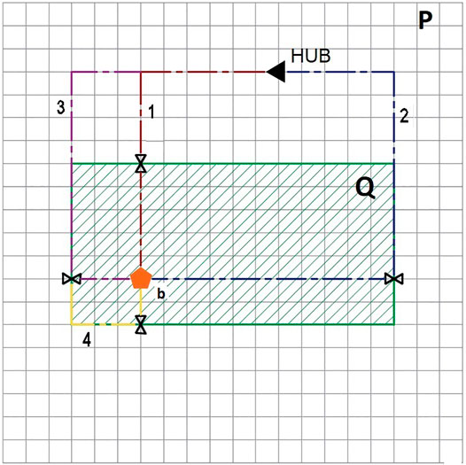
FIGURE 2. Case 2: Customer b located in high-intensity Zone Q.

In the third case, as visualized in Figure 3, customer c is located on the opposite side of the high-intensity Zone Q. In this case, there are potentially two paths to choose from: Path 1, which is shortest in terms of distance and partially lies inside zone Q, and Path 2, that is also shortest in terms of distance for paths that avoid crossing zone Q. The procedure for determining the path with the minimum expected travel time for this configuration is similar to the one described above.

FIGURE 3

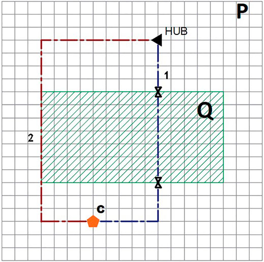
FIGURE 3. Case 3: Customer c located opposite of high-intensity zone Q.

Note that the selection of minimum expected time paths does not guarantee the minimization of the objective function of the RBLMRP, since minimum expected time paths could create additional earliness which may reduce service quality. Hence, we might want to delay the departure from the hub. A corresponding shifting procedure allowing for strategic waiting will be presented in Section 4.3. However, when we performed experiments involving path enumeration, in more than 90% of the instances, the minimum expected travel time paths were the paths selected in the optimal solution.

4.2 Creation of Initial Solution and Tabu Search

Using the procedure described in the previous section, an initial solution is constructed with an insertion heuristic. Our insertion heuristic is based on Solomon (1987) and works as follows. At each iteration of the algorithm, a new customer c ∈ C is assigned to a route r ∈ R that causes the smallest increase in our objective function. For every customer c ∈ C that has not yet been inserted, for every route r ∈ R, every possible insertion position into a route is considered. Then, the best insertion place for a customer c is the one that minimizes the increase in the total value of the objective function. We repeat insertion until all customers have been inserted.

Once we have an initial solution, Tabu Search can be used to improve it. Tabu Search is a well-known metaheuristic method designed to escape local optima. This method was first introduced by Reeves (1993) and has been used to solve many problems, especially vehicle routing problems. The version we use is based on the algorithm by Taş et al. (2013), and we have modified it with respect to the structure and characteristics of our problem, especially with regard to inclusion of pedestrian LOS zones and path selection. The major difference in our Tabu Search and the one in Taş et al. (2013) is that we optimize the robot departure time to minimize our objective. This feature is described in Section 4.3.

At each iteration of the Tabu Search, the algorithm selects a non-Tabu solution from a neighborhood of the current solution which is stored in the candidate list and has a superior value of the objective function relative to the current solution. In case such a solution is not present in the candidate list, the one with the smallest value of the objective function is selected instead. The algorithm runs for a maximum of h iterations or until the solution has not been updated for the last l iterations, where l < h.

Once the new solution is selected, a neighboring solution of the current solution is constructed and added to the candidate list. The neighborhood f(X) of a current solution X is constructed via randomly performing one of the following relocation operators on two randomly selected different customers as follows:

1) Vertex Reassignment. Remove the first selected customer $(\underline{c_2})$ from its current position on a route and insert it into the position after the second selected customer on its route $(\underline{c_4})$, e.g., X = {X₁, X₂}, $X_1=(hub,c_1,\underline{c_2},c_3)$, $X_2=(hub,\underline{c_4},c_5,c_6)\to X_1=(hub,c_1,c_3)$, $X_2=(hub,\underline{c_4},\underline{c_2},c_5,c_6)$.

2) Vertex Swap. Exchange the position of two selected customers on their routes ($\underline{c_2}$ and $\underline{c_4}$), e.g., X = {X₁, X₂}, $X_1=(hub,c_1,\underline{c_2},c_3)$, $X_2=(hub,\underline{c_4},c_5,c_6)\to X_1=(hub,c_1,\underline{c_4},c_3)$, $X_2=(hub,\underline{c_2},c_5,c_6)$.

Note that vertex reassignment can possibly reduce the number of routes and, consequently, the required number of robots activated at the hub.

4.3 Shifting Departure Times to Allow for Strategic Waiting

Once a new candidate solution is created, we perform a shifting procedure on this solution, allowing for strategic waiting of robots at the hub. This is done to improve the balance of earliness and lateness in the objective function. Recall that the path chosen is the one with the minimum expected travel time, so a delay at the hub may improve the objective. In this procedure, we examine the best delay, in multiples of M minutes, for the first customer on the route that optimizes the service quality for the entire route. Note that this yields an approximation of the optimal shift only. In evaluating the service quality associated with this shift, if the departure time for a customer c is shifted by a value of k_cM, k_c > 0, then the arrival time for all the subsequent customers will also be shifted by the same value. We repeat this process for the remaining customers on the first route, and then repeat this process for additional routes. The procedure outlined below is different from the one performed in Taş et al. (2013), who perform only one shift before the vehicle leaves the depot.

Algorithm 1

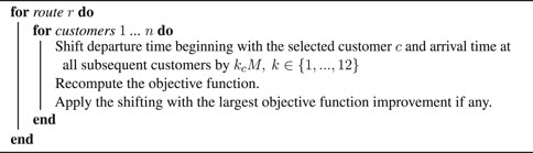
ALGORITHM 1. Shifting procedure

To illustrate the shifting mechanism, consider the following example. Assume a robot has to service the customers c₁, c₂, c₃ in the given order. Next, assume that after performing the shifting procedure for c₁, i.e., shifting all customers starting with c₁ by k, by evaluating the resulting solutions, we found that k ∈ (1, … , 12) represents the best shifting in terms of the objective function is k₁M. So, the arrival times for customers become shifted by k₁M. Further assume that a similar procedure for c₂ results in k₂M being the best shifting, so, the arrival time for customer c₂ and c₃ are now (k₁ + k₂)M later than in the original version of the solution. Repeating this for c₃ yields the following shifts in arrival times for all customers: k₁M for c₁, (k₁ + k₂)M for c₂ and (k₁ + k₂ + k₃)M for c₃.

5 Computational Results

In the following section, we introduce the design of our computational experiments and discuss our results. We are particularly interested in the impact of the pedestrian LOS zones on path selection and objective function values.

5.1 Design of Experiments

Our delivery area is represented by a 2∗2 km square with 100*100 m blocks. Following the description of our problem in Section 4, we divide the delivery area into two pedestrian LOS zones P and Q, where Q represents a high-intensity LOS zone located in the inner zone as depicted in Figure 1. The customer locations are randomly distributed at the corner points of the blocks. In our experiments, we use Manhattan distances between all of the nodes, which reflect sidewalk usage of robots.

We consider two sizes of instances: small instances with 20 customers and large instances with 50 customers. We also consider two different customer densities in the inner zone: for sparse instances, 33% of the customers are located inside Q; for dense instances, 67% are located inside Q. This creates four different types of instances. For each, we create 10 random customer locations per instance, resulting in 40 different instances. Then, for each instance, we assign two variants of customer time windows. First, we consider one-hour time windows (8–9; 9–10 … 14–15, 15–16) for all customers, and second, one-hour time windows for customers located in P and two-hour time windows (8–10; 10–12; 12–14; 14–16) for customers located in Q. The latter instances will be used to help us understand if wider time windows in high-intensity pedestrian LOS zones can help us achieve better service quality values (i.e., less earliness and lateness).

To investigate the effect of potentially higher pedestrian-intensity levels in the inner zone, we consider the following scenarios, which represent several travel time distributions per unit of distance in Q and follow the LOS categories as presented by Burden (2006):

1) Free Flow (low intensity). This defines our base case. It corresponds to the situation when the pedestrian LOS in Q is the same as in P and there is no pedestrian-induced congestion on the sidewalk. Travel times per unit distance are Gamma distributed with the following shape and scale coefficients: T∼Γ(1, 1), representing LOS “A” as described by Burden (2006).

2) Congested Zone (average intensity). In this scenario, a higher number of pedestrians are observed in Q compared to P, which leads to an average-intensity LOS zone Q. Travel times per unit distance in Q are Gamma distributed with the following shape and scale coefficients: T∼Γ(2, 1), representing LOS “C” as described by Burden (2006). Travel times in P are the same as in the Free Flow scenario.

3) Stop-and-Go Zone (high intensity). A very high number of pedestrians is observed in Q compared to P. Travel times per unit of distance in Q are Gamma distributed with the following shape and scale coefficients: T∼Γ(4, 1), representing LOS “E” as described by Burden (2006). Travel times in P are the same as in the Free Flow scenario.

Note that we use the Free Flow scenario as benchmark for all our metrics. We do not compare to a fleet of conventional trucks since Bakach et al. (2021) already show the superiority of robot fleets on last mile deliveries in a two-tier system without LOS zones. To keep computational results comparable across the experiments, we activate the same number of robots for every data set: three robots for the small instances and seven robots for the large instances. Following current industry standard as discussed in Bakach et al. (2021), robots are assumed to move with a speed of 3 km/h. For the Tabu Search algorithm, we use the following parameters: maximum number of iterations h = 200, maximum number of iterations without solution improvements l = 30, shifting multiple M = 5 min. Instances with 20 customers required up to 30 min, and 50 customers instances could be solved within 4 hours run time. The algorithm was coded in Python.

5.2 Results

First, we present the results for instances where all customers have one-hour time windows. Then, we present the results with extended time windows.

5.2.1 Summary of Results One-Hour Time Windows

A summary of results is provided in Table 1. Results are aggregated according to the considered travel time scenario (“Free Flow” vs. “Congested Zone” vs. “Stop-and-Go Zone”). We present the average objective function values (obj), the average percentage increase of the objective function compared to the Free-Flow scenario (% obj Δ), the average total distance traveled by all robots (km), the average total distance traveled in the inner zone (Q Dist) and the outer zone (P Dist) if applicable, the average percentage of distance traveled in the inner (%Q km) and the outer (%P km) zones, the average expected total travel times in hours (time), the average expected travel time in the inner (Q time) and outer (P time) zones, and the average percentage of expected travel time in the inner (%Q time) and the outer (%P time) zones.

TABLE 1

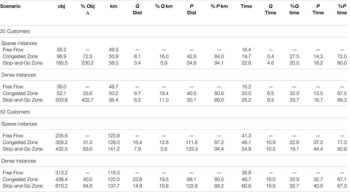
TABLE 1. Summary results.

There are several important observations. For all instances, the objective values increase significantly from Free-Flow to Stop-and-Go scenarios. This is mainly due to increasing scale values of the Gamma distribution, which lead to higher (and more realistic) expected travel times and travel time variations in the congested and stop-and-go scenarios. With small instances of 20 customers, there is more than a 400% increase for the dense instances and over 200% for sparse instances. This indicates a dramatic loss in service quality associated with Stop-and-Go Zones, especially when the majority of customers are located in the pedestrian zone. With an increase in the number of customers and resulting economy of scale, the percentage objective function increase is not quite as pronounced with 50 customers and is at most 95% for dense instances. The absolute changes in the objective, though, are even larger with the large 50 customer instances. Across the set of experiments, the increase in the objective function highlights the importance of considering pedestrian LOS on earliness and lateness for both the Congested Zone and Stop-and-Go scenarios. This indicates it is very important for companies to consider LOS in their service design and service promises.

Next, we will examine the percentage of distance traveled inside the zones. With slightly less than 20% of total distance traveled in Q in case of the Congested-Zone scenario, the number drops to 11% (Stop-and-Go dense) and even to 5.9% in case of sparse instances for the Stop-and-Go Zone with 20 customers. These drops are similar for 50 customer instances. These values indicate that the paths selected are indeed ones that tend to avoid Q in the more congested scenarios, indicating the importance of considering pedestrian traffic in the route planning for robots.

We also investigate the changes in the selected path type and the related distances. Recall that we defined the different path candidates in Section 4.1, with Type-1–Type-4 paths depicted in Figure 2. A summary of results is provided in Table 2. The results reflect that the majority of the paths selected are Type-1 paths, which are the distance-shortest paths. However, the precise percentage is heavily influenced by the scenario. For example, in the case of the Congested Zone, Type-1 paths are selected at only around 88% of the time, leading to an increased distance of 1.5–1.6 km for 20 customers and 4.1–5.7 km for 50 customers on average; for the Stop-and-Go Zone, the number is even smaller at around 67%, leading to an increased distance of 7.7–8.7 km for 20 customers and 17.3–21.4 km for 50 customers on average. This indicates a change to paths that may travel a longer distance to avoid the LOS zones. This is an important tradeoff for companies to consider.

TABLE 2

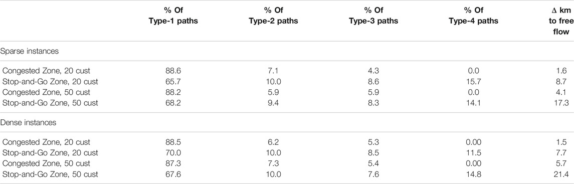
TABLE 2. Distribution of selected paths to in-zone customers.

Results for Type-4 paths exhibit a most interesting result. In the case of the Congested Zone scenario, these paths are never selected; however, in the case of the Stop-and-Go Zone scenario, they are selected at the highest rate compared to all other paths excluding Type-1 paths across all instance types. The explanation might be the following: despite increasing expected travel times (and variance) in the Congested Zone scenario, it might still be worth taking a path that has a significant portion of it lying in Q. However, when pedestrian intensity rises significantly, at some point, it becomes beneficial to avoid Q as much as possible. Companies need to understand these “breakpoints” for the customers they serve.

A visual example is provided in Figure 4. In Figure 4A, we observe the situation for the Free-flow LOS. Since the pedestrian intensity across the whole square is the same, there is no differentiation between zones, and paths of Type 1 are always selected. In Figure 4B, a congested Zone scenario is introduced. As a result, the paths selected to serve the customers that are close to zone edges change, however, the impact of the zone is not significant enough to alter all paths. In Figure 4C, a Stop-and-Go Zone instance is depicted. It can be seen that the Stop-and-Go pedestrian traffic leads to changing paths avoiding robot presence inside the zone.

FIGURE 4

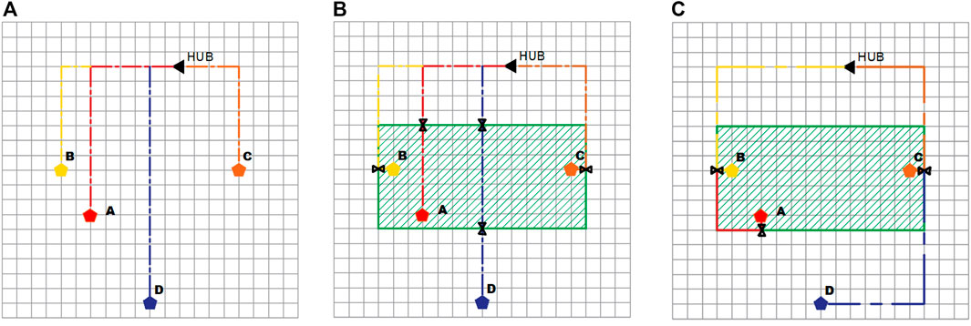
FIGURE 4. Paths Demonstrating the Impact of Different Zones: (A) Free Flow, (B) Congested Zone, (C) Stop-and-Go Zone.

5.2.2 Results With Extended Time Windows

We present the results with extended time windows for Congested and Stop-and-Go scenarios in Table 3. In this experiment, we intend to see if larger time windows reduce the increase in objective functions seen in the previous section.

TABLE 3

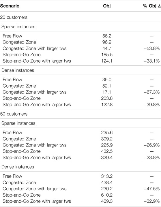
TABLE 3. Objective function comparisons between 1-hour time windows and extended inner zone time windows.

Computational results show a consistent pattern of smaller objective values for the instances with the 2-hour time windows. On average, objective function values are around 20–65% smaller compared to 1-hour time windows across all instances with larger reductions for the Congested Zone scenarios. In fact, across all four instance types, the service quality, as measured by the objective is better for the congested zone with larger time windows than for the free flow zone with the 1 hour time window (e.g. 44.7 $<$ 56.2). These results indicate that larger customer time windows may improve customer satisfaction in terms of reducing earliness and lateness where there is high pedestrian density. It is important for companies to evaluate whether their customers would be willing to accept the wider time window promise given it is more likely to be achieved on time.

6 Conclusions and Future Work

In this research, we have investigated the impact of zones with high pedestrian intensity on customer service levels for last-mile deliveries with ground-based robots in the presence of stochastic travel times and soft customer time windows. We have shown that the existence of zones with different pedestrian LOS can significantly alter the path selection process and affect the customer service level. Our results demonstrate the impact of different levels of the presence of pedestrians for ground-based robot deliveries. We present results with changes in the objective of over 400%. We also show high-intensity zones impact the optimal path from the hub to the customer. This situation is more pronounced for Stop-and-Go Zone scenario where Type-4 paths are being chosen despite the fact they are never preferred for other instances. In addition, we show that if customers are willing to expand expected delivery time windows, the resulting customer service level might increase significantly by up to 40%. All of these results reveal important trade offs for companies to consider when examining the use of robots in urban environments.

There are plenty of future avenues for this research. First, we would like to extend our path finding and routing methodology in the direction of matheuristics and/or exact models, which would improve the quality of the solutions determined in this paper and more directly address the complex objective function of balancing earliness and lateness in a stochastic environment. In this context, we would also like to consider algorithmic and implementation improvements to decrease the computation time for larger data sets. Second, we would like to investigate the impact of the multiple zones on the routing of ground-based robots in conjunction with multiple routes as presented by Bakach et al. (2021). It would be interesting to consider several possible robot hub locations in order to explore which customers should be served from which hub in light of the pedestrian zones. Also, we would like to investigate the generalizability of our approach in real-world networks. Third, in many cases, pedestrian LOS are time-dependent, with peak and off peak pedestrian levels. We would like to look at different ways to model this time dependency to explore how it can potentially impact ground-based robots, including ways of modelling travel times beyond expected values as presented in this paper. Fourth, we would like the consider the possibilities of dynamic hub location for daily optimization of this influential decision. Finally, integration of robot-based deliveries within omni-channel environments and into managing customer acceptance decisions might be worthwhile to make sure delivery capacity is appropriate for demand.

Data Availability Statement

The original contributions presented in the study are included in the article/Supplementary Material, further inquiries can be directed to the corresponding author.

Author Contributions

IB was responsible for modeling, writing, algorithm design, and implementation. AC and JE were responsible for the concept, modeling, results interpretation, and revising the paper.

Conflict of Interest

The authors declare that the research was conducted in the absence of any commercial or financial relationships that could be construed as a potential conflict of interest.

Publisher’s Note

All claims expressed in this article are solely those of the authors and do not necessarily represent those of their affiliated organizations, or those of the publisher, the editors and the reviewers. Any product that may be evaluated in this article, or claim that may be made by its manufacturer, is not guaranteed or endorsed by the publisher.

Supplementary Material

The Supplementary Material for this article can be found online at: https://www.frontiersin.org/articles/10.3389/ffutr.2021.773240/full#supplementary-material

References

Bakach, I., Campbell, A. M., and Ehmke, J. F. (2021). A Two-Tier Urban Delivery Network with Robot-Based Deliveries. Networks 78 (4), 461–483. doi:10.1002/net.22024

CrossRef Full Text | Google Scholar

BBC (2018). Robot Company Starship Technologies Start milton Keynes Deliveries. Available at: https://www.bbc.com/news/uk-england-beds-bucks-herts-46045365?fbclid=IwAR3Cc48-HnJrE1C3eoMyxLPZo3tai9Macab7dkynUALUBoCjVHK383Ly4pA.

Google Scholar

Behnke, M. (2019). “Recent Trends in Last Mile Delivery: Impacts of Fast Fulfillment, Parcel Lockers, Electric or Autonomous Vehicles, and More,” in Logistics Management (Springer), 141–156. doi:10.1007/978-3-030-29821-0_10

CrossRef Full Text | Google Scholar

Boysen, N., Fedtke, S., and Schwerdfeger, S. (2020). Last-mile Delivery Concepts: a Survey from an Operational Research Perspective. OR Spectr., 1–58. doi:10.1007/s00291-020-00607-8

CrossRef Full Text | Google Scholar

Boysen, N., Schwerdfeger, S., and Weidinger, F. (2018). Scheduling Last-Mile Deliveries with Truck-Based Autonomous Robots. Eur. J. Oper. Res. 271 (3), 1085–1099. doi:10.1016/j.ejor.2018.05.058

CrossRef Full Text | Google Scholar

Burden (2006). New York City Pedestrian Level of Service Study Phase I. Available at: https://www1.nyc.gov/assets/planning/download/pdf/plans/transportation/td_fullpedlosb.pdf.

Google Scholar

Christian, A. W., and Cabell, R. (2017). “Initial Investigation into the Psychoacoustic Properties of Small Unmanned Aerial System Noise,” in 23rd AIAA/CEAS aeroacoustics conference, 4051. doi:10.2514/6.2017-4051

CrossRef Full Text | Google Scholar

Ehmke, J. F., Campbell, A. M., and Urban, T. L. (2015). Ensuring Service Levels in Routing Problems with Time Windows and Stochastic Travel Times. Eur. J. Oper. Res. 240 (2), 539–550. doi:10.1016/j.ejor.2014.06.045

CrossRef Full Text | Google Scholar

Ehmke, J. F., Steinert, A., and Mattfeld, D. C. (2012). Advanced Routing for City Logistics Service Providers Based on Time-dependent Travel Times. J. Comput. Sci. 3 (4), 193–205. doi:10.1016/j.jocs.2012.01.006

CrossRef Full Text | Google Scholar

FAA (2018). Small Unmanned Aircraft Regulations (Part 107). Available at: https://www.faa.gov/news/fact_sheets/news_story.cfm?newsId=22615.

Google Scholar

Figliozzi, M. A. (2020). Carbon Emissions Reductions in Last Mile and Grocery Deliveries Utilizing Air and Ground Autonomous Vehicles. Transportation Res. D: Transport Environ. 85, 102443. doi:10.1016/j.trd.2020.102443

PubMed Abstract | CrossRef Full Text | Google Scholar

Grazia Speranza, M. (2018). Trends in Transportation and Logistics. Eur. J. Oper. Res. 264 (3), 830–836. doi:10.1016/j.ejor.2016.08.032

CrossRef Full Text | Google Scholar

Hu, M. (2020). China’s E-Commerce Giants Deploy Robots to Deliver Orders amid Coronavirus Outbreak. Available at: https://www.scmp.com/tech/e-commerce/article/3051597/chinas-e-commerce-giants-deploy-robots-deliver-orders-amid.

Google Scholar

Hu, W., Dong, J., Hwang, B.-g., Ren, R., and Chen, Z. (2019). A Scientometrics Review on City Logistics Literature: Research Trends, Advanced Theory and Practice. Sustainability 11 (10), 2724. doi:10.3390/su11102724

CrossRef Full Text | Google Scholar

Hussain, R., and Zeadally, S. (2018). Autonomous Cars: Research Results, Issues, and Future Challenges. IEEE Commun. Surv. Tutorials 21 (2), 1275–1313. doi:10.1109/COMST.2018.2869360

CrossRef Full Text | Google Scholar

IEEE (2020). Self-driving Robots Hitting london Streets for a New Trial. Available at: https://robots.ieee.org/robots/starship/#:∼:text=Starship%20is%20a%20six%2Dwheeled,Year%202015%20Type%20Consumer%2C%20Delivery.

Google Scholar

Janjevic, M., Winkenbach, M., and Merchán, D. (2019). Integrating Collection-And-Delivery Points in the Strategic Design of Urban Last-Mile E-Commerce Distribution Networks. Transportation Res. E: Logistics Transportation Rev. 131, 37–67. doi:10.1016/j.tre.2019.09.001

CrossRef Full Text | Google Scholar

Jennings, D., and Figliozzi, M. (2019). Study of Sidewalk Autonomous Delivery Robots and Their Potential Impacts on Freight Efficiency and Travel. Transportation Res. Rec. 2673 (6), 317–326. doi:10.1177/0361198119849398

CrossRef Full Text | Google Scholar

Kok, A. L., Hans, E. W., and Schutten, J. M. J. (2012). Vehicle Routing under Time-dependent Travel Times: the Impact of Congestion Avoidance. Comput. Operations Res. 39 (5), 910–918. doi:10.1016/j.cor.2011.05.027

CrossRef Full Text | Google Scholar

Marble (2020). Marble. Available at: https://www.marble.io/.

Google Scholar

McKinsey and Company (2016). Parcel Delivery the Future of Last Mile. Available at: https://www.mckinsey.com/\\∼/media/mckinsey/industries/travel\\%20transport\\%20and\\%20logistics/our\\%20insights/how\\%20customer\\%20demands\\%20are\\%20reshaping\\%20last\\%20mile%20delivery/parcel_delivery_the_future_of_last_mile.ashx.

Google Scholar

Ostermeier, M., Heimfarth, A., and Hübner, A. (2021). Cost-optimal Truck-And-Robot Routing for Last Mile Delivery. Networks. doi:10.1002/net.22030

CrossRef Full Text | Google Scholar

Poeting, M., Schaudt, S., and Clausen, U. (2019). “Simulation of an Optimized Last-Mile Parcel Delivery Network Involving Delivery Robots,” in Interdisciplinary Conference on Production, Logistics and Traffic (Springer), 1–19. doi:10.1007/978-3-030-13535-5_1

CrossRef Full Text | Google Scholar

Rajabi-Bahaabadi, M., Shariat-Mohaymany, A., Babaei, M., and Vigo, D. (2019). Reliable Vehicle Routing Problem in Stochastic Networks with Correlated Travel Times. Oper. Res., 1–32. doi:10.1007/s12351-019-00452-w

CrossRef Full Text | Google Scholar

Reeves, C. R. (1993). Modern Heuristic Techniques for Combinatorial Problems. John Wiley & Sons.

Google Scholar

Rice, S. (2019). Eyes in the Sky: The Public Has Privacy Concerns about Drones. Available at: https://www.forbes.com/sites/stephenrice1/2019/02/04/eyes-in-the-sky-the-public-has-privacy-concerns-about-drones/#6ede64d46984.

Google Scholar

Robby (2020). Robby Technologies. Available at: https://robby.io/.

Google Scholar

Russell, R. A., and Urban, T. L. (2008). Vehicle Routing with Soft Time Windows and Erlang Travel Times. J. Oper. Res. Soc. 59 (9), 1220–1228. doi:10.1057/palgrave.jors.2602465

CrossRef Full Text | Google Scholar

Sasso, M. (2018). There Aren’t Enough Drivers to Keep up with Your Delivery Lifestyle. Available at: https://www.bloomberg.com/news/articles/2018-06-13/amazon-grubhub-boom-fuels-cold-dinner-woes-and-hunt-for-drivers.

Google Scholar

Simoni, M. D., Kutanoglu, E., and Claudel, C. G. (2020). Optimization and Analysis of a Robot-Assisted Last Mile Delivery System. Transportation Res. Part E: Logistics Transportation Rev. 142, 102049. doi:10.1016/j.tre.2020.102049

CrossRef Full Text | Google Scholar

Solomon, M. M. (1987). Algorithms for the Vehicle Routing and Scheduling Problems with Time Window Constraints. Operations Res. 35 (2), 254–265. doi:10.1287/opre.35.2.254

CrossRef Full Text | Google Scholar

Sonneberg, M.-O., Leyerer, M., Kleinschmidt, A., Knigge, F., and Breitner, M. H. (2019). “Autonomous Unmanned Ground Vehicles for Urban Logistics: Optimization of Last Mile Delivery Operations,” in Proceedings of the 52nd Hawaii International Conference on System Sciences. doi:10.24251/hicss.2019.186

CrossRef Full Text | Google Scholar

Starship (2020). Starship Technologies. Available at: https://www.starship.xyz.

Google Scholar

Sulleyman (2017). Self-driving Robots Hitting london Streets for a New Trial. Available at: https://www.independent.co.uk/life-style/gadgets-and-tech/news/hermes-self-driving-delivery-robots-london-starship-technologies-a7687161.html.

Google Scholar

Taş, D., Dellaert, N., Van Woensel, T., and De Kok, T. (2013). Vehicle Routing Problem with Stochastic Travel Times Including Soft Time Windows and Service Costs. Comput. Operations Res. 40 (1), 214–224.

Google Scholar

USPS (2018). Summary Report: Public Perception of Delivery Robots in the united states. Available at: https://www.oversight.gov/sites/default/files/oig-reports/RARC-WP-18-005.pdf.

Google Scholar

Wong (2017). Delivery Robots: a Revolutionary Step or Sidewalk-Clogging Nightmare?. Available at: https://www.theguardian.com/technology/2017/apr/12/delivery-robots-doordash-yelp-sidewalk-problems.

Google Scholar

Zhang, S., Campbell, A. M., and Ehmke, J. F. (2019). Impact of Congestion Pricing Schemes on Costs and Emissions of Commercial Fleets in Urban Areas. Networks 73 (4), 466–489. doi:10.1002/net.21872

CrossRef Full Text | Google Scholar