A simulation model of the real-world fuel and energy consumption of light-duty vehicles

1 Introduction

The European Commission proposes to update the 2030 carbon dioxide (CO₂) emissions standards for new passenger cars and light commercial vehicles (vans) registered in the European Union (EU) to a reduction of 55% compared to 2021, as defined in the Fit for 55 package under the European Green Deal (European Commission, 2021), and to a reduction of 100% by 2035. The main intention of lowering the CO₂ emission standards is to reduce global warming induced by greenhouse gas (GHG) emissions from road transport and eventually mitigate climate change. In the EU, light-duty vehicles (LDV) are responsible for 14.5% of the total CO₂ emissions (European Commission, 2022) and relevant standards for the reduction of CO₂ emissions are in place based on a reproducible laboratory type-approval process. However, in real-world driving, a wide range of different operating conditions can occur, such as traffic and ambient conditions, road conditions and gradient (Fontaras et al., 2017b), which no test procedure can adequately cover. In addition, an individual driving style, either smoother or more aggressive, may be followed. This variability in operating conditions results in a 15%–20% difference between the real-world CO₂ emissions and the type-approval test over the Worldwide harmonised Light vehicle Test Procedure (WLTP) (Dornoff et al., 2020).

The divergence between type-approval and real-world CO₂ emissions, which is not stable but has been increasing over the years is a major issue in the effort to reduce CO₂ emissions. For this reason, the European Commission has implemented vehicle fuel and energy consumption monitoring through an On-Board Fuel and/or Energy Consumption Monitoring (OBFCM), mandatory for all new light-duty vehicle registrations since 2021 (Regulation (EU) 2018/1832; Regulation (EU) 2019/631). Such measures aim at monitoring on-road emissions for tracking performance towards the set targets. Alongside, there has been a growing interest in the creation of low-emission zones in city centres by municipality authorities (CLARS, 2022), in an attempt to abate both air pollution and climate change.

Independently from the regulatory actions, an important parameter is the user’s impact on fuel/energy consumption. Towards this, the European Commission and other authorities support actions that aim at raising user awareness to choose fuel/energy-efficient vehicles and at educating users about a more ecological driving style and habits. The Joint Research Centre of the European Commission (JRC, 2016) has presented the Green Driving tool, with which the user can select a vehicle, pick a route, calculate fuel/energy consumption over the selected route and propose alternative routes if available. The users can insert several technical parameters, while some aspects are predefined based on the vehicle segment. IFPEN has developed Geco Air (IFPEN, 2021), a smartphone application focusing on pollutant emissions and training users to drive and commute in an environmentally friendly way. The user provides data related to vehicle characteristics, while the global positioning system of the phone provides the route. This enables the calculation of several parameters, such as NO_x emissions but, the user has limited control over other parameters. Similarly, the MILE21—LIFE project (MILE21, 2019) aimed at informing users about their fuel/energy consumption and providing ways to reduce it by offering a find-a-car tool and fuel/energy consumption self-reporting tool. The first one assists the users in finding a fuel/energy-efficient vehicle that would suit their needs, while the self-reporting tool allows them to record their consumption and benchmark it against an ecological driving style. Both tools deliver representative values of the expected on-road conditions, calculated through vehicle simulation.

The current paper presents the developed tool capable of simulating vehicle representative on-road fuel and energy consumption values at minimal calculation time. The tool uses generic data regarding vehicle fuel consumption and drivetrain losses, based on findings of previous studies regarding fuel consumption calculation using generic data (Samaras et al., 2018; Doulgeris et al., 2020; Zacharof et al., 2020). Both conventional and electrified powertrains are covered over a wide range of operating conditions. Regarding implementation, the tool has low processing needs and is suitable for integration into online platforms. The tool has already been deployed in the MILE21—LIFE platform (MILE21, 2019) to provide representative on-road fuel and energy consumption values using the bare minimum inputs, demanding low effort from the average driver/user. Despite that, the tool offers the possibility to define specific cases (regarding the velocity profile, vehicle load or driving behaviour) and calculate the fuel/energy consumption for such cases. In addition, the tool has further capabilities as it is easy to deploy in other applications. Having this in mind, it was designed to be easily expandable to new technologies with the use of modules and utilizes actual routes by enabling linking with an Application Programming Interface (API). With a recalibration, it is also possible to extend its use to vehicle markets other than the European, as it has been demonstrated for the US market. In addition, future developments can be incorporated since the tool can be easily trained and hence automatically updated by utilizing OBFCM data. This capability is necessary, especially for hybrid powertrains, where it could be possible to improve the generic energy management strategy by developing a vehicle specific strategy. The importance of this capability lies in the fact that hybrid vehicles are expected to play a crucial role in transitioning to fully electric vehicles.

2 Methods

2.1 Model description and development workflow

2.1.1 Background approach and workflow

The current section outlines the workflow followed in the development of the simulation tool that calculates fuel/energy consumption and CO₂ emissions based on vehicle technical characteristics and a given route. For a better understanding of the development process, it is important to clarify key terms as they are used in this work.

The term “simulation model” refers to a software tool that calculates energy consumption and emissions for a given driving route, based on vehicle technical characteristics. If no specific software is referenced, the “simulation model” or simply “model” refers to the tool developed in this work. The term “vehicle model” refers to a set of vehicles that share common characteristics and market name under a manufacturer’s brand. In “vehicle modelling,” on the other hand, technical characteristics of a vehicle model and operating conditions are parametrized to be used as inputs to the simulation model. Regarding the route, the “mission profile” refers to the combination of vehicle speed and road slope values.

The simulation model developed in the context of this study, utilizes two approaches, a physical and a statistical which are applied in parallel and complement each other. The basic theory for these two approaches is described in the work of Treiber and Kesting (2013), where the physical approach considers the vehicle’s longitudinal dynamics, while the statistical approach is a phenomenological model for fuel consumption prediction. Vehicle longitudinal dynamics is used to calculate the energy required for vehicle propulsion and hence, it requires the calculation of the traction force $\left(F_{tr}\right)$, i.e., the force needed to maintain a constant speed—as well as accelerate or decelerate—and which is calculated using the well-known Eq. 1. The equation takes into account aerodynamic drag $\left(F_{aero}\right)$, rolling resistance $\left(F_{fr}\right)$, inertia force $\left(F_{in}\right)$, and slope $\left(F_{slope}\right)$, which are summed together to obtain the traction force at a specific velocity $\left(v\right)$.

$F_{tr}=F_{fr}+F_{aero}+F_{slope}+F_{in}=\mu M_{veh}gcos\left(\phi \right)+\frac{1}{2}\rho c_{d}A{v}^2+M_{veh}gsin\left(\phi \right)+M_{veh}\frac{dv}{dt}(1)$

$M_{veh}$: mass of the vehicle (kg)

$\phi$: angle equivalent to the road grade (rad)

$g$: acceleration of gravity, 9.81 m/s²

$\mu$: rolling resistance coefficient (−)

$\rho$: air density (kg/m³)

$c_d$: aerodynamic drag coefficient (−)

$A$: frontal area (m²)

The parameters $\mu ,c_d,A,M_{veh}$ can be used for calculating the so-called road load coefficients and are characteristic of each vehicle model. Regulation (EU) 2017/1154 considers a standard $\rho =1.21$ kg/m³ and defines the road loads as $F_0=\mu M_{veh}$ and $F_2=\frac{1}{2}\rho c_{d}A$.

Eq. 1 is multiplied by the vehicle speed to calculate the required power. In order to translate this value to the actual fuel/energy consumption from the vehicle’s fuel tank or battery, the losses in the powertrain are needed. These depend on different conditions such as vehicle speed and can be accounted for through an efficiency factor as shown in Eq. 2. The term $P_{tr}$ represents only the traction power, any additional power loss related to auxiliaries (e.g., air conditioning) can be included in Eq. 2 by adding this power to the $P_{tr}$.

$P_{tr}=F_{tr}v=n_{eff}{\dot{m}}_{fuel}LHV\Rightarrow {\dot{m}}_{fuel}=\frac{P_{tr}}{n_{eff}LHV}{P}_{tr}=F_{tr}v=n_{eff}{P}_{bat}\Rightarrow P_{bat}=\frac{P_{tr}}{n_{eff}}(2)$

$P_{tr}$: traction power (kW)

$n_{eff}$: efficiency factor (−)

${\dot{m}}_{fuel}$: fuel flow rate (kg/h)

$LHV$: fuel lower heating value (kWh/kg)

$P_{bat}$: battery power (kWh)

An additional method to calculate fuel consumption is the statistical approach that was also applied in a complementary way to the physical approach. This is based on the calculation of fuel consumption using a polynomial function (Treiber and Kesting, 2013) that utilizes velocity, acceleration and road slope as inputs. The polynomial fit of Eq. 3 is similar in shape to the longitudinal dynamics equation and the regression coefficients $\left({\beta }_n\right)$ resemble the physical parameters of Eq. 2. This way, even though these coefficients are statistical values, they include a variable efficiency.

${\dot{m}}_{fuel}={\beta }_0+{\beta }_{1}v+{\beta }_2{v}^2+{\beta }_3{v}^3+{\beta }_{4}v\frac{dv}{dt}+{\beta }_{5}v\phi (3)$

The efficiency factor $\left(n_{eff}\right)$ of Eq. 2 for ICE includes the engine $\left(n_{eng}\right)$ and transmission $\left(n_{trans}\right)$ efficiencies. Evidently, the efficiency factor depends on the technical characteristics of each vehicle model, such as engine type (Otto or Diesel), capacity, power, tuning, etc. Naturally, the calculation of the fuel consumption using Eq. 2 requires the efficiency factor along with the vehicle specifications and mission profile. Similarly, fuel consumption calculation using Eq. 3 requires as input the mission profile and the regression coefficients (${\beta }_n$).

Ideally, each vehicle model should have a set of efficiency factors ($n_{eff}$ ) for every operating condition ($v,dv/dt,\phi$), as depicted in Eq. 2. The same applies to the $\left({\beta }_n\right)$ coefficients, which may be constant for the different operating conditions, however, they are different for each vehicle model. Nonetheless, it would not be feasible to measure or model in-detail all available vehicle models in the market and cover all possible operating conditions. It was considered that vehicles sharing common characteristics could be grouped as their technical parameters are represented by similar values such as fuel/energy consumption maps, e.g., vehicles from different brands sharing the same engine. For this reason, the European market car models were allocated into clusters and for each cluster, a generic vehicle was created with representative technical characteristics. Subsequently, efficiency factors over a wide range of conditions were calculated using the simulation approach described in-detail below. Despite the generic vehicles do not correspond to actual market-available passenger cars, they function as a proxy to assess actual vehicle behaviour on-road. In this way, the actual vehicle efficiency parameters can be eventually calculated from the generic ones.

Therefore, the current work focused on a few generic vehicles that covered the majority of market-available vehicles. The generic vehicles were simulated in AVL Cruise, a commercially available software, under a wide range of operating conditions (road load and mass value sets and mission profiles). Subsequently, solving Eq. 2 using the simulated fuel consumption provided a dataset of efficiency factors for different operating conditions, which are expressed collectively from traction power $\left(P_{tr}\right)$. This essentially created a matrix of efficiency factors covering all operating conditions, road loads and masses. It is important to state that the derived efficiency factors originate from the fuel consumption and transmission efficiency maps that were introduced in Cruise vehicle models. This means that any technology included in the utilized (fuel consumption and efficiency) maps, is transferred to the calculated efficiency factors.

Using the same simulated vehicle models’ results, the dataset of the regression coefficients $\left({\beta }_n\right)$ was also derived using polynomial multilinear regression for the calculated fuel consumption, velocity, acceleration and road slope. The result of this regression was the set of ${\beta }_n$ coefficients for each generic vehicle. The statistical model was trained for each road load and mass value set $\left(F_0,F_2,M_{veh}\right)$ simulated over specific mission profiles (analysed in the text below). Finally, the derived efficiency factors and regression coefficients are correlated with $F_0,F_2,M_{veh}$ and the mission’s profile driving style. The correlation, described in detail in the following sections, resulted in formulas that provide the efficiency factors $\left\{n_{eng},n_{trans}\right\}$ and ${\beta }_n$ coefficients as a function of vehicle characteristics and driving conditions. Thus, it is possible to calculate efficiency factors and regression coefficients for any actual vehicle and subsequently calculate fuel consumption for any mission profile using Eqs 2, 3.

The simulation model calculates the fuel consumption using both approaches, which complement each other. The physical approach is mainly used for fuel consumption calculation as the utilized efficiency factors inherently contain engine technologies such as cylinder deactivation and valve timing, via the use of engine fuel and gearbox efficiency maps in vehicle modelling. Eq. 3 is employed for calculating fuel consumption under conditions where the accuracy of Eq. 2 is notable limited. Initial validation of the fuel consumption calculation using Eq. 2 revealed diminished accuracy during deceleration phases attributed to fuel cut-off. This discrepancy is primarily ascribed to the need for an additional function in the physical approach to accommodate this technological aspect. In this way, Eq. 2 is used to calculate fuel consumption under all conditions except for deceleration phases, where fuel cut-off occurs. In these phases, Eq. 3 is used, as it better incorporates the effect of this technology. That way, the final fuel consumption calculation is realized with the application and combination of both approaches.

The simulation model development workflow is presented in detail in Figure 1.

FIGURE 1

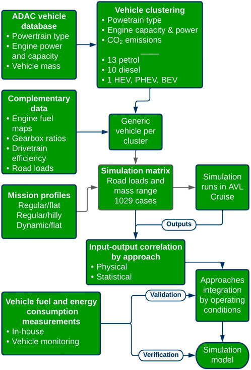
FIGURE 1. Simulation model development workflow.

The steps followed for the development of the simulation model can be summarized as follows:

• Step 1: Market analysis and clustering. A market analysis was performed to identify the passenger car types that are in use in Europe. The goal was to identify vehicle clusters that share similar characteristics regarding the body, powertrain and drivetrain. Each cluster was represented by a generic vehicle.

• Step 2: Simulation cases. Definition of the simulation cases that were subsequently executed using detailed vehicle modelling developed for the generic vehicles. The simulation cases covered a range of road load and mass values and different mission profiles.

• Step 3: Utilization of the simulation results and their correlation with the varied input parameters. At this step, the database with efficiency values and the polynomial coefficients was developed forming the core of the simulation model.

• Step 4: Model validation. The accuracy of the simulation model’s calculated fuel/energy consumption values was determined with measurements. The simulation model was used to replicate the fuel consumption for the mission profiles recorded during the experimental campaign. Subsequently, the calculated fuel consumption was compared with the measured to evaluate the model’s performance.

• Step 5: Model application. The model was used to calculate the overall fuel consumption for vehicles that were monitored for a period of time. In addition, to evaluate the transferability of the model, the fuel consumption of vehicles belonging to the US fleet was calculated. This was preformed to evaluate the model’s capabilities to replicate the fuel consumption of vehicles that have different calibration than those found in the European market.

2.1.2 Vehicle clustering

Step 1 (see Figure 1 above) included an analysis of the market and vehicle grouping. To that aim a vehicle database containing technical characteristics and sales information for the majority of vehicle models available in the European market was obtained from the German automotive club “Allgemeiner Deutscher Automobil-Club” (ADAC). The ADAC vehicle database was analysed extensively in a previous study (Bieker and Diaz, 2021) and was found to contain more than 10,000 vehicle models on sale in Germany since 2013. Despite containing vehicle sales from Germany only, it was found that it was representative of the European fleet, therefore vehicle clustering is considered to be applicable for Europe. The vehicles were grouped into clusters based on powertrain and engine capacity—if available—as further described below. Additional details are also available in 10.1 in the Supplementary Material.

Conventional vehicles were grouped into several different clusters to account for the variety of ICE and transmissions that affect efficiency factors $\left(n_{eng},n_{trans}\right)$. BEVs, PHEVs and hybrid electric vehicles (HEV) did not present such high variability in the period our study was conducted, therefore each of these powertrain types was assigned a single cluster. In hybrid powertrains, the internal combustion engines did not present high variability either to justify further clustering. Although different engine sizes are used in different vehicle bodies and powertrains, the energy management control of hybrid powertrains typically aims to best ICE efficiency. As a result, the operating points of the ICE may be limited to specific points that ensure optimal efficiency (Ichikawa et al., 2017; Kato et al., 2017). Future development could consider expanding the hybrid cluster, especially if more manufacturers offer a wider range of hybrid powertrains and they do not shift their focus on battery electric vehicles. Similarly, for pure electric vehicles, the efficiency maps of the electric machines and the battery characteristics have also low variability, and the parameters mostly affecting electrical consumption are vehicle mass and road load.

In the simulation runs presented in the next section, clusters with low market shares that contained mainly over- or underpowered vehicles of both powertrains were excluded from the Cruise simulations to optimise the necessary effort. Table 1 displays the 5 plus 4 clusters for conventional petrol and diesel models respectively that were finally included in the simulation runs. In the same table the engine displacement, power and official CO₂ emissions bin ranges, along with the minimum and maximum road load and mass values are provided.

TABLE 1

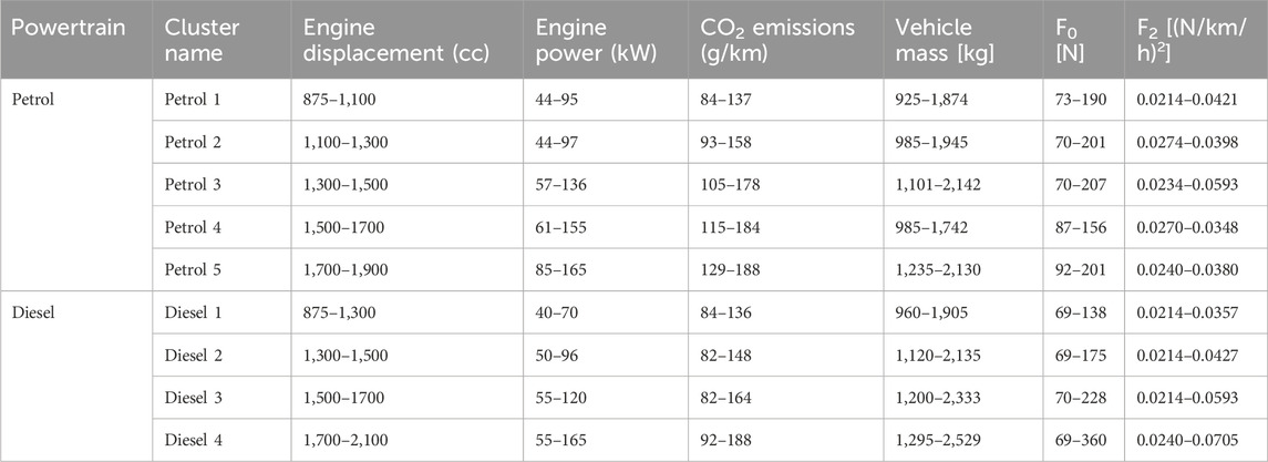
TABLE 1. Clusters for conventional petrol and diesel vehicles.

2.1.3 Model and simulation cases development

As mentioned above, the clusters’ representative generic vehicles were in detail simulated with the Cruise simulation platform. Cruise simulations with cluster representative generic models were performed to obtain the efficiency and fuel consumption calculations for a large dataset of vehicles. That way, it was made possible to obtain a combination of mass and road loads that are representative of the range for each cluster. The necessity for these simulations arose as a means to replace the labor-intensive experimental campaigns that would otherwise be essential to comprehensively address all vehicle clusters and their respective vehicles. In essence, these simulations can be regarded as intelligent tools for interpolation and extrapolation, enabling the generation of a more substantial dataset to populate each cluster. Since the ADAC database did not comprise all the required simulation inputs, such as engine fuel consumption maps and road load values $\left(F_0,F_2\right)$, additional vehicle data was acquired from other available sources. The EPA database (EPA, 2021) provided the required road load values for each vehicle model. Moreover, the overall Cruise model layout was based on template models, while the engine fuel consumption maps and vehicle component characteristic curves and efficiency maps were derived based on generic approaches developed in previous studies (Tsokolis et al., 2015; Samaras et al., 2018; Doulgeris et al., 2020). The development of the generic vehicles’ fuel consumption maps was based on scaling models of actual vehicles in Cruise, which was done by applying the Willans lines approach, as detailed in prior research (Sorrentino et al., 2015; Tsiakmakis et al., 2017). For instance, a measured engine fuel consumption map of 1,300 cc was scaled to 1,200 cc for the simulation needs of the Petrol 2 cluster generic vehicle. The detailed vehicle modelling process also accounted for the transmission efficiency via the gearbox efficiency map, the calculation of which drew from a method outlined in Zacharof et al. (2020). Following this methodology, the generation of gearbox efficiency maps makes a distinction between manual and automatic transmission. This process produced one single generic vehicle for each cluster with representative engine, transmission, mass and road load values. Figure 2 presents an example of a typical vehicle simulation model topology in AVL Cruise based on which the clusters’ representative models were built.

FIGURE 2

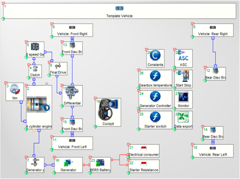
FIGURE 2. Typical vehicle simulation model topology in AVL Cruise.

Based on the vehicle clusters, the road load (F₀ and F₂ coefficients) and mass series were combined to form a matrix that resulted in 343 vehicle configurations for each generic vehicle. Each parameter varied according to the range of the vehicle cluster, and the combinations represented a different vehicle or vehicle configuration. The 343 cases derived by the F₀, F₂ and mass variations, were combined with 3 different mission profiles.

The mission profiles comprised different speed profiles (representing a driving style) and routes that present different terrain morphology. Driving style with acceleration and deceleration values well within the Real-Driving Emissions (RDE) regulation was considered regular or normal, and it was combined with a flat and a hilly route. Higher absolute acceleration/deceleration values were considered as dynamic driving and were combined only with a flat route. Although dynamic driving could occur over any route, it was considered that it would be less frequent over a hilly route for safety reasons. Therefore, the dynamic/hilly combination was excluded to reduce the computational effort. Hence three mission profiles were considered, which combined with the vehicle configurations resulted in a simulation matrix of 1,029 cases for each generic vehicle.

The gear selection was taken into consideration in the simulation model by choosing a representative gear-shifting pattern for each generic vehicle and mission profile (regular, dynamic, hilly) taking that way also into account the interlink between driving style and gear selection. The gear-shifting pattern was extracted following the provisions of the WLTP (Regulation (EU) 2017/1151) and it was provided as input along with the velocity and road grade profile in Cruise. For the generic vehicles that deployed automatic gearboxes—as they were representative of their cluster—the gear-shifting was also extracted following the WLTP provisions.

The cases matrix was used to run simulations in Cruise that introduced realistic vehicle operation by implementing a driver model expressed with an appropriate gear-shifting strategy for each mission profile. For each simulation case, the runs delivered time-series of $v,P_{TR},{\dot{m}}_{fuel},n_{eng},n_{trans},\phi$.

Additional energy consumption from auxiliaries such as air conditioning was not included in the simulations at this stage, there was a lack of suitable measured data for calibration and validation. Since the impact of air-conditioning alone can lead to an increase of up to 10% in fuel/energy consumption (Fontaras et al., 2017b) in conventional vehicles and account for much more in electric ones, it was decided to address the topic in the future.

2.1.4 Correlation of simulation results with the input parameters

As described above, the correlation between the simulation case inputs and outputs (simulation results) was performed using a physical and a statistical approach, both applied for each generic vehicle, considering as inputs the road load and mass values shown in Eqs 4, 5.

The simulation results for each generic vehicle were segmented by mission profile (i.e., driving style) and route type (urban, rural, highway). The separation between urban, rural and highway is based on vehicle speed $\left(v\right)$ with the respective bins being [0, 60) [60, 90) and ≥90 km/h. The driving style (dynamic or normal driving) is determined based on acceleration $\left(a=\frac{dv}{dt}\right)$ and particularly utilizing the product of vehicle speed and acceleration ($v\bullet a$). The 95^th percentile of the positive $v\bullet a$ was compared with the limits of the RDE regulation to characterize the dynamicity. The closer to the limit, the more aggressive the driving style. However, the dynamicity limits are not stable and are determined based on the route segment’s average vehicle speed. A more detailed description is included in section 10.2 of the Supplementary Material. Finally, the hilliness was defined from the slope $\left(\phi \right)$ with segments having a positive elevation gain of 850 m/100 km being considered as hilly. This way, each mission profile delivered three segments based on the route type resulting in a total of 9 types of segments (3 mission profiles × 3 route types). Segmenting the results facilitated the correlation between inputs and outputs thanks to the more or less homogenous conditions within each segment. Subsequently, an average efficiency value was calculated for each segment type.

As a result, the regression coefficients (a, a', b, b', c, c', d, d') are derived for each cluster and segment type by applying a multilinear regression to the inputs from the simulation runs $\left(F_0,F_2,mass\right)$ enabling the calculation of powertrain efficiency and ${\beta }_{\mathrm{i}}$ coefficients for any combination of inputs and subsequently, fuel and energy consumption.

${\mathrm{n}}_{\text{eff}}=\mathrm{a}{F}_0+b{F}_2+c{M}_{veh}+d(4)$

${\beta }_{\mathrm{i}}={\mathrm{a}}^{\prime }{F}_0+b^{\prime }{F}_2+c^{\prime }{M}_{veh}+d^{\prime }(5)$

a, a', b, b', c, c', d, d': regression coefficients (−)

2.1.5 Integration of electrified powertrains

Vehicles with an electrified powertrain were simulated using an additional sub-model that implements an operational strategy. The generic simplified energy management strategy (EMS) introduced for PHEVs and HEVs, deploys charge-depleting and charge-sustaining modes, with Figure 3 presenting the conditions under which each mode is deployed. During charge-depleting mode, the vehicle is considered to be moving with pure electric driving, while during charge-sustaining mode the vehicle is assumed to enter the hybrid operation with either battery charging or discharging.

FIGURE 3

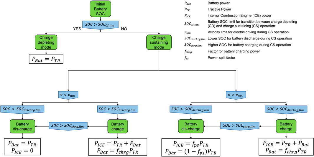
FIGURE 3. Generic strategy applied for the plug-in hybrid and hybrid vehicles.

The decision for the transition between charge-depleting and charge-sustaining mode is made based on the battery state of charge (SOC) which is calculated using Eq. 6 where C is the nominal capacity of the high-voltage battery in kWh and SOC is expressed as a percentage of the nominal battery capacity (0%–100%). SOC thresholds are used to define when the vehicle operates in charge-depleting mode or when to engage the internal combustion engine. The decision margins could differ depending on the battery size (PHEVs have larger batteries compared to HEVs).

$SO{C}_i=SO{C}_{i-1}+100\frac{P_{bat}}{3600s}\cdot \frac{1}{C}(6)$

A PHEV operates as pure electric in charge-depleting mode until the battery is depleted below the transition SOC threshold when the vehicle enters charge-sustaining mode and the internal combustion engine starts. During charge-sustaining mode, the battery SOC oscillates in a bandwidth, e.g., 11%–12% for PHEVs. HEVs on the other hand which have no off-grid charging, are associated with rather limited pure electric driving and as they have smaller batteries this bandwidth is in the range of 40%–50% SOC. The selection of theses thresholds was made based on experimental data from (P)HEV testing and considered as generic, representative values.

In charge sustaining mode, engagement of the internal combustion engine is not only related to the SOC but also to power demands. For this reason, there is also a controller for the vehicle speed where the maximum speed of electric driving is 50 km/h, while for a velocity above 80 km/h, the battery is charged by the ICE. This feature is mainly applicable to HEVs, where due to the low nominal capacity, it is possible to re-charge the high voltage battery, at a significant level, using the ICE. At that vehicle speed, the ICE can reach optimum operating conditions directing some of the power in vehicle propulsion and the remaining to charge the battery, thus making more efficient use of the fuel. In these cases, battery charging above 80 km/h continues until the SOC charge limit is reached. Again, these velocity thresholds were selected as representative generic values, extracted from experimental data. With this approach, it is possible to capture the battery charging using the electric motor and the torque assist, by increasing or decreasing the power demand from the ICE. The amount of power used to assist the ICE or added to the ICE for battery charging is controlled by the $f_{ps}$ (Power split factor) and the $f_{chrg}$ (Factor for battery charging power) respectively. This factor was extracted from the experimental campaign with the electrified vehicles. During laboratory testing the standard emissions measurement set-up was enhanced with the introduction of a power analyser which allowed the measurement of the currents and voltages from the electric machine(s) and high voltage battery. Using the power analyser recordings, the electric power of the electric components was calculated, making possible (using also the power on wheels demand and engine power whenever was calculation was possible) the investigation of the power flow and power split within the different components of the powertrain. Hence, these two factors are expressed as the fraction of the tractive power request and were selected empirically from experimental data and calibrated during model development. Finally, during deceleration, the inertia force is used to charge the battery simulating the regenerative braking.

2.2 Model integration

The simulation model is a comprehensive tool that integrates various aspects required for calculating fuel and energy consumption in a streamlined process. Figure 4 illustrates the internal steps that the model takes to produce the required values using decision-making processes on different levels.

FIGURE 4

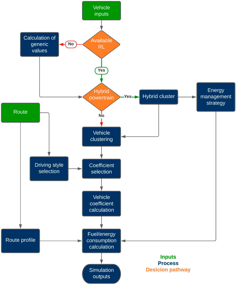
FIGURE 4. Simulation model structure.

The simulation model requires minimum inputs, such as vehicle technical characteristics (brand, model, powertrain, fuel type, engine details, weight, dimensions), route data (time, speed, altitude, driving style, share of urban/rural/motorway) and, if available, optional inputs like road loads $\left(F_0,F_2\right)$, frontal area and aerodynamic drag. Initially, the tool checks for road load values; if absent, it selects generic road load values based on similar vehicles and adjusts them according to curb weight and dimensions or frontal area inputs. For hybrids, the model allocates them to the respective cluster with an energy management strategy, while conventional vehicles are allocated based on the engine details. Generic coefficients are selected based on route and vehicle attributes, considering factors like road slope and driving style. Fuel/energy consumption calculations involve traction power, consideration of coasting and/or fuel cut-off conditions, and the implementation of the energy management strategy for hybrid powertrains. The goal of the simulation model is to calculate the fuel/energy consumption of a passenger car under real-world conditions for a specific mission profile, or typical real-world fuel/energy consumption values (based on a representative mission profile).

An example of the steps to calculate fuel consumption with the simulation model include:

• retrieval of the vehicle’s engine characteristics, fuel type, road loads and mass and allocation of the vehicle in a cluster; separation of the route in segments based on route type, hilliness and driving style dynamicity

• for each segment, calculation of an average efficiency factor and $b_i$ coefficients according to its type utilizing the regression coefficients for the physical and statistical approach

• then calculation of the traction power for every timestamp along the route

• derivation of the fuel consumption

To illustrate the efficiency factor and $b_i$ coefficients calculations, an example follows that considers an actual petrol vehicle with 1,200 cc engine displacement, 55 kW power, $F_0=136$ N, $F_2=0.04214$ N/(km/h)² and $M_{veh}=992$ kg, which is classified in the Petrol 2 cluster. The vehicle is driven over a specific route, which is segmented as shown in Figure 5.

FIGURE 5

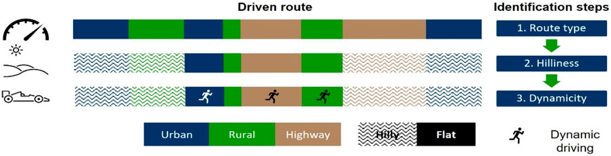
FIGURE 5. Route segmentation according to vehicle speed, hilliness and driving style.

The route is separated into urban, rural and highway segments based on the vehicle speed. Subsequently, based on the slope calculated from the GPS signal each segment is classified as flat or hilly. In the third step, the dynamicity is determined for the flat segments.

Finally, for each segment, the regression coefficients a, b, c, and d are chosen for each segment type and the average efficiency is calculated based on Eq. 4. Similarly using the a', b', c', d' for each segment type the $b_i$ coefficients are calculated with Eq. 5. The efficiency values for each segment of Figure 5 route are shown in Table 2.

TABLE 2

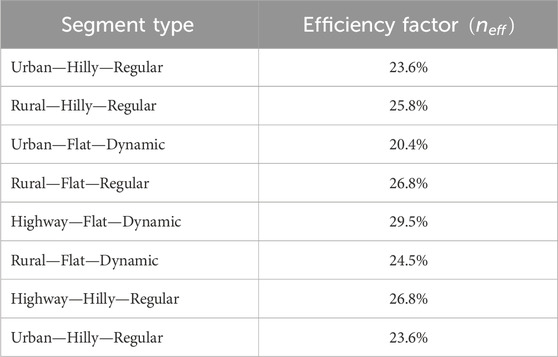
TABLE 2. Calculation of efficiency factor by segment type for the example.

The efficiency values vary for the same mission profile due to the road load and mass combinations that lead to different ICE operating points. In order to visualize this, an example is provided for the Petrol 2 cluster. Figure 6 displays the calculated efficiency factors, representing both “low” and “high” combinations where efficiency ranges between 18.7% and 33%. These combinations correspond to the minimum and maximum road load and mass within the cluster. Previous studies by Fontaras et al. (2017a) and Pavlovic et al. (2018) have also reported similar trends. Improved efficiency values over highway driving, which are further improved with dynamic driving style are also expected due to the engine functioning on a more optimal operating range (Rodríguez-Fernández et al., 2022).

FIGURE 6

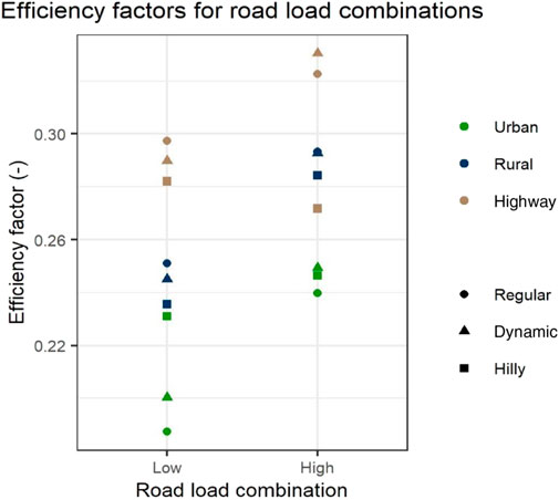
FIGURE 6. Efficiency factor for minimum and maximum road load/mass combinations for Petrol 2 cluster.

As described earlier, efficiency factors for each route segment and generic vehicle were calculated utilizing a representative gear-shifting strategy. Therefore, the simulation model does not consider any gear-shifting pattern for the calculation of the fuel consumption at user-inserted routes.

For each route segment (regular, dynamic, hilly), the allocated efficiency factors inherently include transmission efficiency, which is also affected by the gear-shifting strategy. However, as described earlier, efficiency factors for each route segment and generic vehicle were calculated utilizing a representative gear-shifting strategy. Therefore, the simulation model does not consider differences in gear-shifting at user-inserted routes as such an approach would require the user to also introduce engine speed along with the mission profile. Naturally, this would be a complicated process for the average user. In addition, it would also be out of the scope of the current work as it would increase the calculation time, which is not desirable for an online platform. Future research that includes further improvements for expert users could develop a gear-shifting feature.

In the case of a (P)HEV, the sub-model for electrified vehicles is enabled. The selection and calculation of the coefficients is the same as for the conventional vehicles derived from the xEVs’ cluster though. In addition to the fuel consumption calculation, the EMS decision process is enabled along with the SOC and energy consumption calculation.

2.3 Vehicle measurements

Fuel and energy measurements were conducted through an extensive experimental campaign, comprising on-road and laboratory testing. Target of the measurements was to obtain data to validate the fuel consumption prediction performance of the simulation model. Diverse vehicle types and powertrains were tested under various operating conditions to ensure data coverage. An additional monitoring scheme involved actual users with logging devices recording consumption and other operating parameters.

2.3.1 In-house measurements

The measurements included both real-world and WLTP testing on a chassis dynamometer using the standard CVS (Constant Volume Sampling) methodology recording instantaneous and bag concentrations of CO₂ and pollutant emissions (CO, NO_x, HC, PM). On-Board Diagnostic (OBD) data, including engine speed, velocity, intake mass flow, control module voltage and fuel rate, were recorded using a generic OBD scan tool. On-road tests deployed a Portable Emissions Measurement System (PEMS) for measuring CO₂ and pollutant emissions along with an exhaust flow meter (EFM) to measure the exhaust mass flow rate. For both laboratory and on-road testing, instantaneous fuel consumption was calculated utilizing the recorded concentrations of CO₂, CO, and HC based on the carbon balance method following the calculation methodology in Regulation (EU) 2017/1151. The baseline route and driving style were designated following the RDE regulations, while additional conditions such as uphill/downhill routes and different driving styles, based on similar approaches (Dimaratos et al., 2019; Triantafyllopoulos et al., 2019; Zacharof et al., 2020; Toumasatos et al., 2022) were also considered for testing. Table 3 presents a description of the on-road tests performed.

TABLE 3

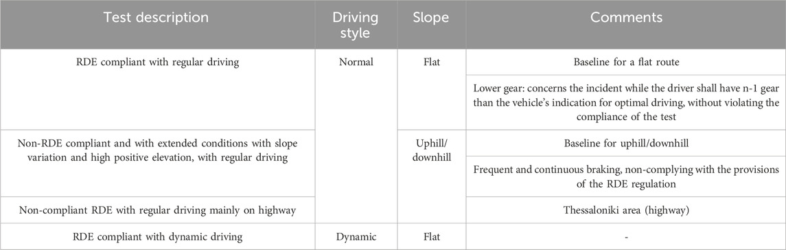
TABLE 3. Overview of performed on-road tests.

Figure 7 presents the on-road testing routes: (A) represents the RDE-compliant route, (B) extends the route to include higher road gradients and (C) presents a custom route emphasizing highway driving with varying road slopes. The figure also includes the mission profiles—namely, the vehicle speed and altitude profiles along the routes—that offer insights into the testing conditions and terrain characteristics.

FIGURE 7

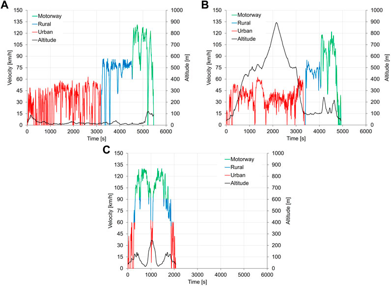
FIGURE 7. On-road test routes mission profiles, (A) RDE compliant route, (B) route that includes uphill and downhill driving, (C) route with mainly highway driving including uphill and downhill.

Eight vehicles—whose main specifications are presented in Table 4 were used for the experimental campaign that covered a wide range of the most popular market segments. In total, 29 on-road tests with petrol and 19 with diesel vehicles were performed, which included different driving patterns.

TABLE 4

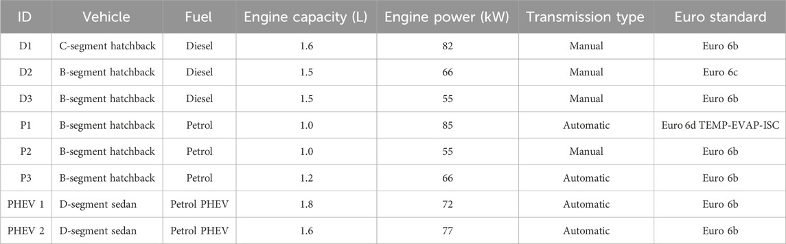
TABLE 4. Technical characteristics of measured vehicles.

2.3.2 Vehicle monitoring

In addition to PEMS testing, another set of measurements was carried out as part of the MILE21 project. This was a long-term monitoring initiative focusing on actual users and their driving behaviours, aiming to capture real-world data. For this reason, OBD loggers were installed to record information regarding the driving style and fuel consumption directly from the vehicle’s OBFCM. These measurements played a crucial role in the verification of the model, effectively assessing its performance across a broader spectrum of vehicles and driving conditions. Table 5 provides an overview of the vehicles included in the monitoring scheme equipped with OBFCM devices.

TABLE 5

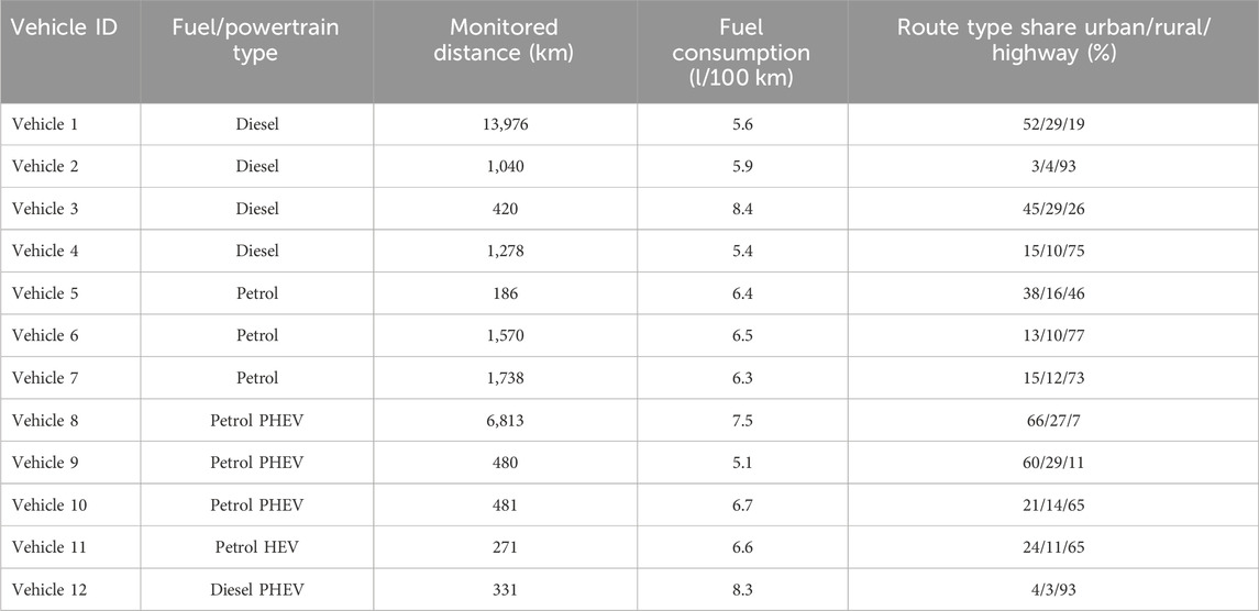
TABLE 5. Monitored vehicles with OBFCM.

Throughout the monitoring process, the installed loggers were transmitting OBD data via a wireless connection, with all data promptly stored in a database. These signals included velocity, engine speed, fuel consumption and other parameters relevant to the operation of the powertrain. The recording frequency was 1 Hz. In addition to capturing instantaneous data, the loggers also tracked cumulative values over the lifetime distance and fuel/energy consumed.

It should be highlighted that the OBFCM ensured that fuel/energy consumption was within ±5% accuracy as required by Regulation (EU) 2018/1832. While the regulation established these accuracy standards for reference fuel and vehicle wheels, market fuel blends can introduce variations that may impact accuracy. However, the study by Dornoff and Zacharof, 2022 confirmed the accuracy of the OBFCM with market fuels showing expected variations of up to ± 3.9% in petrol and ±3.3% in diesel vehicles. Post-processing of the recorded data allowed the characterization of each driver’s driving style (normal, dynamic) the determination of the proportion of urban, rural and highway driving, as well as the calculation of the total fuel consumption.

2.4 Model application

2.4.1 Measurement and monitoring data verification

The accuracy of the fuel consumption calculation model was further assessed using on-road monitoring data. From this dataset, it becomes possible to compute the proportions of urban, rural and highway driving, which are then utilized as inputs to the model. Consequently, the total fuel consumption was calculated by knowing the vehicle specifications and driving styles of each driver (inferred from recorded velocity).

To predict real-world fuel consumption, a representative mission profile is employed, with adjustments made to align with the urban, rural and highway driving shares. It is worth noting that an alternative approach could involve using the actual recorded velocity profile. However, this approach proved to be insufficient due to extended monitoring periods, often spanning many hours or even days. The purpose of this verification using real-world data was to assess the model’s performance when confronted with limited input data. It is essential to emphasize that the outputs of fuel consumption calculation models, akin to the one presented in the study, exhibit high sensitivity to the input data. The choice between a generic or actual vehicle profile can yield notable variations in the results (Mogno et al., 2020).

2.4.2 US fleet

To demonstrate the model’s versatility beyond its applicability to EU passenger cars, the model was utilized to calculate CO₂ emissions for United States (US) cars using data provided by the Environmental Protection Agency (EPA). The choice of the United States was motivated by its position as one of the largest vehicle markets worldwide—along with China and Europe—with new annual vehicle registrations of about 5 million passenger cars and 12 million light trucks (NTS, 2019).

It is important to note that vehicle segment definitions in the United States differ from those in Europe. In the United States, the term “passenger car” includes vehicles with car-like body types and gross vehicle weight (GVW) of up to 3,900 kg, as well as two-wheel drive SUVs of up to 2,700 kg. In contrast, the term “light trucks” includes all vans and four-wheel-drive SUVs up to 4,500 kg GVW and includes cargo vans and pick-up trucks with GVW up to 3,900 kg. While light trucks may be perceived as a separate category, they often function as passenger vehicles (Tietge et al., 2017) and they are included in the EPA database. Consequently, making a direct comparison with the EU passenger car category, which comprises vehicles with a GVW below 3,500 kg and with no more than eight passenger seats, poses challenges. To address this, the current application considered exclusively vehicles with car-like bodies and SUVs with a GVW below 2,700 kg.

The EPA maintains FuelEconomy.gov (US Department of Energy and EPA, 2022), a website designed to assist consumers in making informed vehicle purchasing decisions by providing fuel economy labels. These labels offer representative values of real-world fuel economy in Miles Per Gallon (MPG) (Tietge et al., 2017). Notably, the term “fuel economy (MPG)” in the United States is equivalent to “fuel consumption (l/100 km)”. For consistency, all final values in this study are reported as fuel consumption in l/100 km.

The EPA label values are derived from a series of five laboratory test cycles designed to capture representative real-world conditions. As a detailed description of the EPA methodology is out of the scope of the current work, the EPA provides also a two-cycle approach where vehicles are measured over the Federal Test Procedure (FTP-75) for urban driving and the Highway Fuel Economy Test Cycle (HWFET) for highway driving. Subsequently, post-processing of the measured values proceeds as shown in Eq. 7 to calculate EPA label values.

$\begin{array}{c}{FC}_{city}=\frac{1}{0.004091+\left(\frac{1.601}{{FC}_{FTP-75}}\right)}\\ {FC}_{highway}=\frac{1}{0.003191+\left(\frac{1.2945}{{FC}_{HWFET}}\right)}\end{array}(7)$

FC_city: City fuel consumption (MPG)

FC_FTP-75: FTP-75 fuel consumption (MPG)

FC_highway: Highway fuel consumption (MPG)

FC_HWFET: HWFET fuel consumption (MPG)

The model application focused on simulating FC_FTP-75 and FC_HWFET values for the available vehicles and subsequently applying Eq. 7 in the post-processing. The latter step was needed to enable comparison with the respective EPA label values.

Regarding, the vehicles, the EPA data include vehicle specifications, road loads and test mass for FTP-75 and HWFET cycles, which were utilized as inputs to the model. Vehicles that were not within the boundaries set by the model in terms of capacity, were excluded from the application. The EPA 2020 database contained 764 and 606 test results for the FTP-75 and HWFET cycles respectively (EPA, 2021). Notably, all vehicles were powered by petrol engines as this is the dominant fuel type for passenger cars in the United States.

3 Results and discussion

3.1 Validation with in-house measured vehicles

The simulation model accuracy was validated through a comprehensive process that included measurements from nine conventional vehicles—both petrol and diesel variants—and two electrified vehicles, specifically PHEVs. A total of 73 tests were conducted to assess the model’s accuracy employing various criteria such as total and instantaneous trip consumption by urban, rural and highway parts. The validation is explicitly based on the comparison of the model’s prediction and the fuel consumption obtained from measurements, either from the carbon balance method utilizing emissions recording or the OBFCM reported values from the OBD. Furthermore, the model’s ability to accurately predict the state of charge for electrified vehicles was scrutinized and compared with the experimental recordings.

The model calculated fuel/energy consumption for each measured vehicle and test. The benchmark for model acceptance was defined with a margin of ±10% in comparison to the measured values, a threshold commonly accepted in similar studies (e.g., Mogno et al., 2020).

For clarity, the validation results are presented separately, with an initial focus on conventional powertrains including both petrol and diesel vehicles, followed by an assessment of PHEVs.

As mentioned earlier, the in-house measurements provided detailed data, which could assist in identifying potential issues in the simulation model performance.

Figure 8 shows the distribution of the difference between measured and predicted fuel consumption by fuel type over the whole trip and separated into urban, rural and highway parts.

FIGURE 8

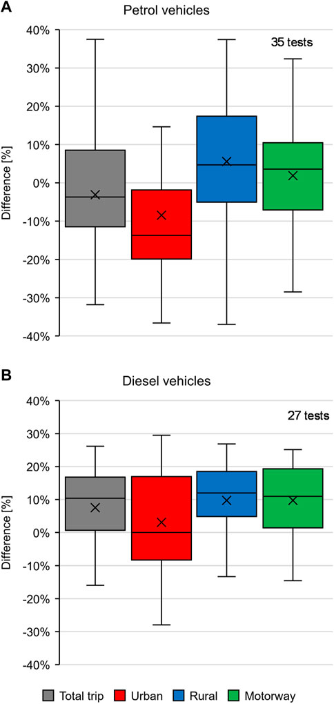
FIGURE 8. Model validation for petrol (A) and diesel (B) vehicles by route type.

For petrol vehicles, the overall (total trip) difference was found between 9% and −11% at 95% confidence interval. Examining differences by route type, rural and highway segments remain within the ±10%, evenly distributed around 0%. However, urban driving tends to underestimate fuel consumption ranging from −2% to −20%. Some of this deviation may be attributed to the cold start, given the urban part occurs at the beginning of the route. The cold start is the phase when vehicle components, such as engine, drivetrain, exhaust after-treatment system, suspension, and tyres have not reached thermally stable operating conditions. During that phase, additional energy (e.g., from the fuel consumption) is required for the component warm-up, or losses (e.g., powertrain) are increased, resulting in higher fuel and electric energy consumption, in the case of electrified powertrains. The additional fuel/energy consumption depends also on the selected thermal management strategy applied to each vehicle.

In contrast, diesel vehicles exhibit an overall trip difference ranging from 1% to 17%. Rural and highway segments tend to overestimate fuel consumption, reaching up to 20% on the highway. Urban routes are associated with a broader range, varying from −8% to 17%.

In order to assess the statistical significance of these differences, a paired t-test was also performed. The t-test considered pairs of measurement and simulation results with an alpha level of 0.05. Table 6 presents the calculated p-values from the t-test performed for each powertrain and route type.

TABLE 6

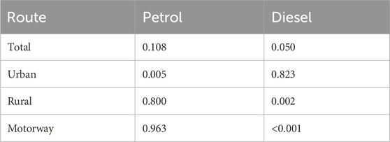
TABLE 6. Calculated p-values from t-test by route type with an alpha level of 0.05.

For the interpretation of the t-test results, p-values higher than the alpha level mean that we can accept the null hypothesis that there is no difference between the two groups.

Regarding petrol vehicles, in almost all cases the p-value is higher than the alpha level, except in the case of the urban segment. This indicates that further work is needed to address shortcomings such as the cold start, which have been highlighted earlier. In the case of diesel vehicles, there is a significant difference in the rural and motorway segments as it has been illustrated also in Figure 8 with the mean differences being −0.34 and −0.45 L/100 km respectively. Further calibration of the tool could improve the results, as, for example, by considering different clustering for diesel vehicles. Nonetheless, the results for the urban segment and total trip showed that the p-value is higher than the alpha level indicating that overall there is a good agreement for the two groups.

Figure 9 compares cumulative and total fuel consumption for the best prediction accuracy cases for petrol (Vehicle A) and diesel (Vehicle B) powertrains. Figure 9A presents the difference between measured and predicted fuel consumption for Vehicle A—the P1 B-segment petrol vehicle with a 1.0 L engine and automatic gearbox (AT)—on a highway route with significant road grade. Figure 9B presents Vehicle B—the D2 B-segment diesel vehicle with a 1.5 L engine and a manual gearbox—driven on an RDE-compliant route with a regular driving style.

FIGURE 9

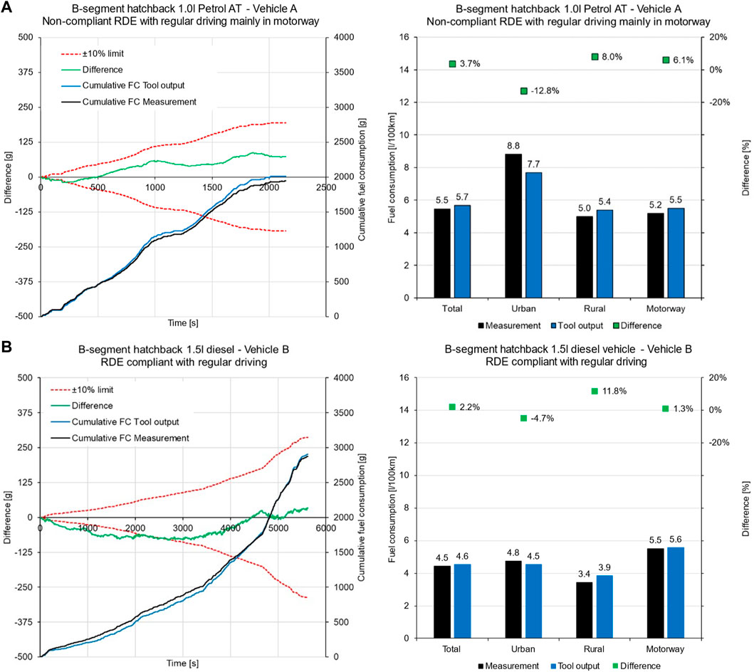
FIGURE 9. Measurement and model prediction cumulative fuel consumption comparison for the best case (A) petrol-Vehicle A-and (B) diesel-Vehicle B-vehicle.

For vehicle A, the model calculations showed good agreement with the measured fuel consumption with an overall difference of 3.7%. However, the urban part of the route showed an underestimation of 13%, while for the rural and highway parts that followed, the divergence after engine warm-up was 8.0% and 6.1% respectively. It was observed that the engine coolant temperature reaches the operating temperature within the first 500–1,000 s of urban driving, but additional effects such as transient operation should also be considered. The warm-up time is also affected by the ambient conditions, driving style and engine thermal management. The cold start effect at a starting temperature of 20°C was calculated at 13% by Fontaras et al., 2017b, which is in line with the difference found in this simulation case. It is worth noting that the model does not currently consider the cold start effect, which could be a potential area for further improvement.

The model prediction for Vehicle-B also presents an underestimation from the beginning of the trip that is consistent for most of the trip. The difference between measured and predicted fuel consumption shifts to the positive side in the middle of the rural part. This divergence cannot be attributed solely to the cold start, and it could originate from other parameters that are related to the calibration of the model. For the total fuel consumption, the divergence between measured and predicted fuel consumption is at 2.2%, while for the rural part, the difference is 11.8%, a value significantly higher compared to the other parts. This value though is balanced out by the lower difference of the urban part, which showed an underestimation of −4.7%, a difference that can be attributed to the cold start effect.

Figure 10 presents the respective results for the worst cases by comparing measured and predicted fuel consumption for two RDE-compliant routes. The vehicles are P3, a B-segment petrol vehicle with a 1.2 L engine (Vehicle C) and D1, a C-segment vehicle with a 1.6 L diesel engine (Vehicle D). Figure 10B sub-plot presents a route with regular driving for Vehicle C, while on the other hand, the sub-plot Figure 10B presents a dynamic driving trip for Vehicle D.

FIGURE 10

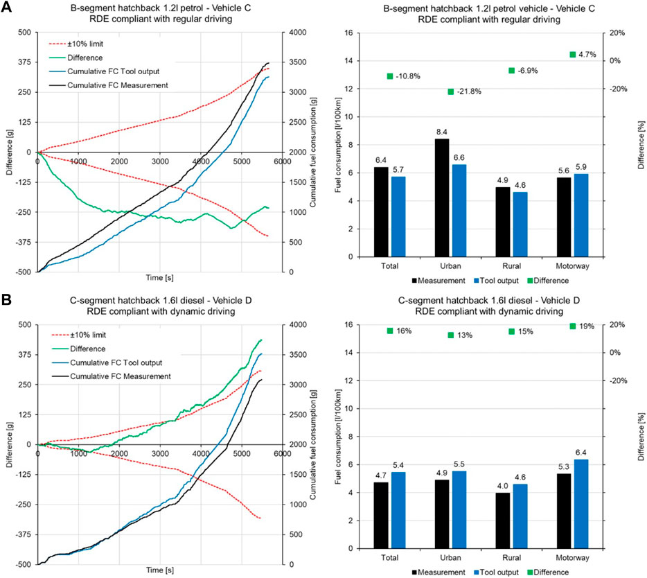
FIGURE 10. Measurement and model prediction cumulative fuel consumption comparison for the worst case (A) petrol-Vehicle C- and (B) diesel-Vehicle D-vehicle.

Vehicle C was an example of a worst-case petrol vehicle simulation, with an overall divergence of −10.8% over the complete trip. It is noteworthy that the rural and highway parts were well within the ±10% threshold with a divergence of −6.9% and 4.7% respectively. In contrast, the urban part exhibited a considerable underestimation of 21.8%. Even when accounting for 13% due to a cold start, the remaining deviation could be attributed to factors such as engine idling and the trip’s dynamic nature of urban driving, characterized by frequent accelerations. Despite being marginal, the whole trip is considered regular driving and this is reflected in the simulation results.

For the diesel vehicles, Vehicle D presented a divergence of 16% over the whole trip. Separating the route into parts showed that the overestimation was constant with 12.6%, 15.2%, and 19.1% respectively over the urban, rural and highway parts. The observed divergence in this case is mainly related to the calibration of the fuel consumption calculation parameters for the cluster that the vehicle belongs to. The trip is characterized by dynamic driving, and after a more detailed investigation, it was observed that by replacing the parameters with those for regular driving, the difference drops to 10%. This means that the efficiency values calculated for the dynamic driving of this cluster are underestimated. The source of this underestimation could be related to the gear selection sequence used for the generic mission profile with dynamic driving, during the training of the model. Eckert et al. (2022) reported that there is a 15.6% benefit in fuel-saving achieved with optimal transmission configuration (number of gears, gear and final drive ratios) and shifting strategy, a value that indicates the high influence of the transmission on fuel consumption. The influence of the gear selection strategy was also investigated during the experimental campaign. Two tests were also performed on the same route with normal driving, but for one of the tests, a late gear upshift was applied by the driver. In these tests, the fuel consumption was 20% higher than the test with the normal gear shift.

At the next step, the model application was investigated on two PHEVs, which posed the challenge of essentially deploying two different power sources: petrol and electricity. Figure 11 presents PHEV A and B over different driving conditions. The vehicles were driven both in charge-depleting—mainly electric driving—and charge-sustaining mode.

FIGURE 11

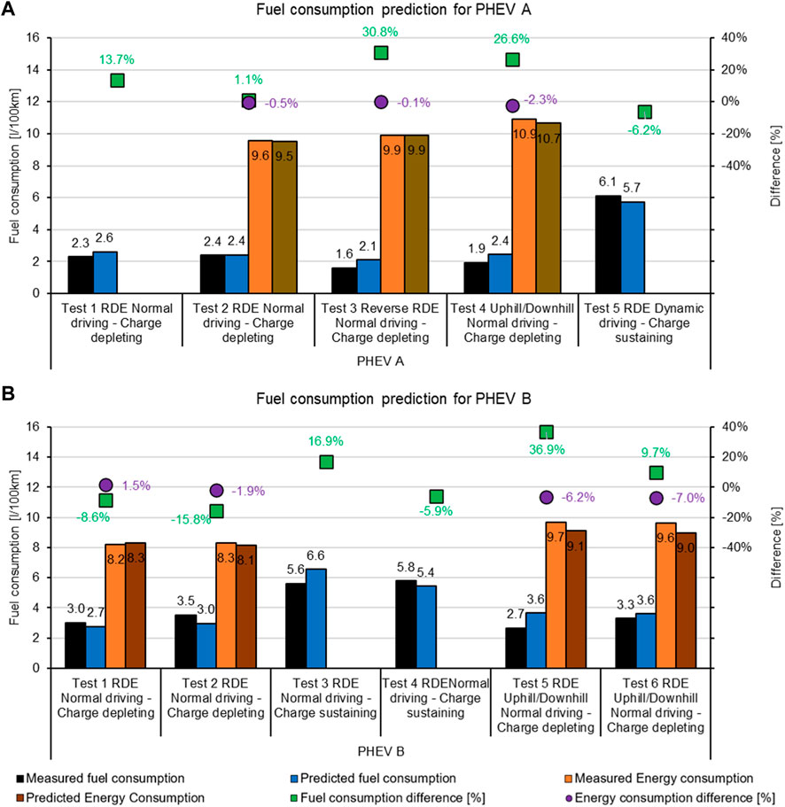
FIGURE 11. Measurement and model prediction of total fuel and energy consumption comparison for PHEV A (A) and PHEV B (B) by route type.

In charge-depleting mode, PHEV A presents an overestimation which could be up to 30.8%. However, it should be highlighted that in these cases, fuel consumption is relatively low, in the order of 2 L/100 km, which could have a disproportionate effect on the relative difference. The maximum absolute difference was 0.5 L/100 km. In charge sustaining mode, the relative difference between prediction and measurement was −6.2% and the absolute value was −0.4 L/100 km. On the other hand, PHEV B predictions presented a different trend. Test 1 and 2, both RDE-compliant routes under normal driving conditions in charge-depleting mode presented an underestimation. Under similar conditions but in charge-sustaining mode, Test 3 presented an overestimation of 16.9%, while Test 4 in and an underestimation of 5.9%. Tests 5 and 6 were both with uphill and downhill driving and presented an overestimation of 36.9% and 9.7%, respectively. However, it is interesting that the model calculated similar fuel consumption at 3.6 L/100 km in both cases, while the measurements delivered values of 2.7 and 3.3 L/100 km.

The model incorporates a generic EMS module that has been experimentally derived and tested to cover various operating conditions. However, the observed variability suggests the need for further optimization and customization of the EMS module for each PHEV. To illustrate this point, Figure 12 depicts the battery state of charge evolution for both measured and predicted values. Specifically, Figure 12A shows the results for PHEV A operating in charge-depleting mode, while Figure 12B shows the corresponding results for PHEV B in charge-sustaining mode.

FIGURE 12

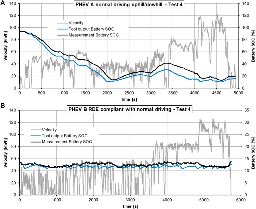
FIGURE 12. Battery stage of charge development for PHEV A (A) and PHEV B (B).

The comparison between the measured and calculated battery SOC for PHEV A revealed fluctuations during the trip. At the end of the trip, the difference was in the order of 4%, which indicates good agreement. However, during uphill driving, the model calculated a rapid decrease in battery charge resulting in higher fuel consumption. At around 2,000 s, the vehicle recovered energy during downhill driving and then entered charge-depleting mode for a short period until 4,200 s, after which it switched to charge-sustaining mode completely. This trend shows that the model overestimated electric energy consumption and recuperated less energy during braking, resulting in higher fuel consumption. When the vehicle entered in charge sustained mode the measured and simulated SOC values converged.

Test 4 of PHEV B also showed good agreement in the SOC evolution over charge-sustaining mode. However, the energy management strategy was not fully captured. The predicted battery SOC fluctuated between the charge (12%) and dis-charge (11%) limit while in the test results, this was not always the case. For example, in the highway measurements between 5,000 and 6,000 s, the recorded battery SOC was rather constant, which was achieved by the synergy between the thermal engine and the electric motor. At this operating point, the thermal engine was used to propel the vehicle, while the electric machine absorbed energy from the engine to power the electric motor assisting in vehicle propulsion. In contrast, the implemented generic strategy applied in the model, during charge sustaining mode always considers either battery charging or battery dis-charging with torque assist.

3.2 Verification with monitored vehicles

The verification of the model’s accuracy in calculating fuel consumption utilized fuel/energy consumption values and vehicle speed from the monitored vehicles’ OBFCM device. The data was categorized into urban-rural-highway parts based on vehicle speed, which the model used to calculate weighted average fuel consumption. Figure 13 shows the difference between the predicted and the measured values for four diesel, three petrol, three PHEV and one HEV.

FIGURE 13

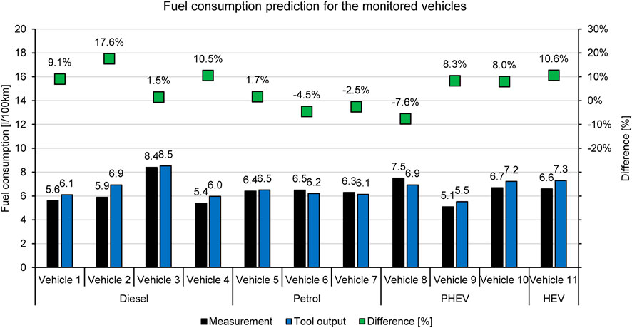
FIGURE 13. Fuel consumption prediction for the monitored vehicles.

The results showed that the model was able to calculate fuel consumption within the error margin of ±10% for most of the cases. However, two cases slightly exceeded this value by ∼0.5%, while one case had a significantly higher divergence reaching up to 17.6%. The high divergence is related to the overall performance of the model for diesel vehicles, where the prediction trends towards the overestimating of fuel consumption.

For petrol vehicles, the trend seems more distributed with values ranging from −4.5% to 1.7%. Mogno et al. (2020) reported similar findings in their study using a similar tool—the Green Driving tool—where they found an average uncertainty of 12% and a bias of up to 3%.

PHEVs showed a wider spread in fuel consumption ranging from −7.6% to 8.3%, but still within the expected margins. This could be attributed to PHEV drivers driving more in charge-sustaining mode than in charge-depleting mode. It has been a common issue that PHEV drivers do not charge their vehicles regularly, which could have an impact on the technology’s expectations to reduce fuel consumption (Plötz et al., 2018). The HEV showed a difference of 10.6%, which was slightly higher than the limit of ±10%.

3.3 US fleet results

The simulation model calculated city and highway fuel consumption for the available US fleet vehicles in an exercise to demonstrate the tool’s capability to extend to another region. This was done to investigate whether is possible to accurately predict the fuel consumption of US vehicles using a tool that is calibrated and validated with vehicles that are from the European market. As a result, the verification with the US data can provide an insight of the additions needed to improve and further extend the developed tool. The results were compared with the respective City and Highway fuel consumption values from the EPA. Figure 14 illustrates the distribution of the divergence between the simulated and the EPA values. Since there was uncertainty regarding hybrid vehicles, the investigation only focused on petrol vehicles.

FIGURE 14

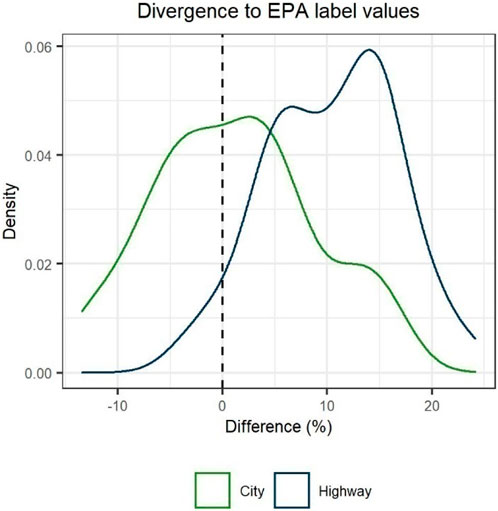
FIGURE 14. Distribution of divergence between predicted and EPA label values.

In the City route, approximately 77% of the vehicles demonstrated fuel consumption estimates within a range of ±10% of the EPA-reported values, with 50.8% of these vehicles with differences within the ±5% margin. The mean difference in this case was only 1.2%, indicating good performance. Conversely, in the Highway route, a larger mean difference of about 10% was observed, with 45.5% of the vehicles falling within the ±10% margin.

The model’s tendency to overestimate fuel consumption during high-speed driving can be attributed to several factors. Firstly, cars sold in the United States generally possess a higher power-to-weight ratio compared to their EU counterparts. Secondly, variations in gear shifting patterns, especially considering the prevalence of automatic gearboxes in the United States compared to the EU, contribute to this. Lastly, the model deploys generic gearboxes representative of EU vehicles, which may deviate from actual US gearboxes. Consequently, if the actual ratios of the two highest gears are below those of the generic gearbox, the model underestimates engine efficiency during highway driving eventually overestimating fuel consumption. A significant portion of the deviation originates from the model’s basis in generic vehicles tailored explicitly to represent the EU fleet.

4 Conclusion

The current work introduced a simulation model for predicting real-world fuel/energy consumption for both conventional and electrified vehicles. This model relies on generic vehicle data and minimal input parameters, while the validation compared the model’s predictions against on-road measurements. The model was applied to vehicle monitoring data to further assess accuracy. The results revealed that the achieved fuel consumption accuracy was within ±10% for a significant portion of the tests used in the validation. The exception was the underestimation of petrol vehicles in the urban part which highlighted the importance of including the cold start effect. There was also an observed overestimation trend for diesel vehicles, suggesting some clustering issues. Nevertheless, the model’s overall performance makes it suitable for deployment in online platforms or similar applications that demand a straightforward and rapid simulation tool. Moreover, its adaptability with the US fleet was demonstrated, although fine-tuning may be required to align with specific fleet characteristics.

Future enhancements to the model could address calculation issues in diesel vehicles and transform it into a comprehensive data-driven model using OBFCM data. One proposal in this direction involves developing a simulation model to obtain OBFCM data from monitored vehicles, subsequently creating an internal database for calculating efficiency coefficients for specific vehicle models to replace generic values. This would yield more accurate representations of each vehicle’s performance compared to the current generic approach. For hybrid powertrains, this solution could also be used to train the EMS and adjust it to specific vehicle models. Furthermore, for hybrid and electric powertrains, expanding clustering to include a broader range of vehicle sizes could be explored. Another potential enhancement involves incorporating a “thermal model module” to assess vehicle warm-up and apply corrections for the cold start effect, which is particularly important for electrified powertrains. Additionally, relative measurements could provide valuable data for auxiliary usage implementation and improved fuel and energy consumption calculation, especially in scenarios where auxiliaries like air-conditioning pose a significant load. Regarding gear-shifting, it could be possible to train the model in a similar way as the OBFCM data by introducing the engine speed and correlating it with the vehicle speed. This could assist in limiting any errors derived from generic gear-shifting.

To enhance its utility, the model could be integrated with an API capable of suggesting fuel/energy-efficient routes based on user-provided origin-destination information. Achieving this would necessitate the development of a “driver module” capable of generating the required speed profile. These proposed enhancements underscore the model’s potential for expansion by incorporating additional modules to improve accuracy.

Data availability statement

The data analyzed in this study is subject to the following licenses/restrictions: The data was provided by ADAC under the agreement that any publication would include aggregated data only. For this reason, the publication includes aggregated data as agreed. Requests to access these datasets should be directed to https://www.adac.de/kontakt-zum-adac/kontaktformulare/test-und-technik/.

Author contributions

NZ: Conceptualization, Data curation, Formal Analysis, Investigation, Methodology, Visualization, Writing–original draft, Writing–review and editing. StD: Conceptualization, Data curation, Formal Analysis, Investigation, Methodology, Visualization, Writing–original draft, Writing–review and editing. AZ: Data curation, Formal Analysis, Methodology, Writing–original draft. AD: Investigation, Validation, Writing–review and editing. RvG: Conceptualization, Methodology, Writing–original draft. SoD: Formal Analysis, Investigation, Writing–original draft. ZS: Funding acquisition, Project administration, Resources, Supervision, Writing–review and editing.

Funding

The author(s) declare financial support was received for the research, authorship, and/or publication of this article. The development of the simulation model was done within the context of the MILE21—LIFE project. The project MILE21 is co-funded by the LIFE Program of the European Union with agreement number LIFE17 GIC/GR/000128. The research work was supported by the Hellenic Foundation for Research and Innovation (HFRI) under the HFRI PhD Fellowship grant (Fellowship Number: 607).

Acknowledgments

The authors would like to acknowledge the support of this work by the personnel of the Laboratory of Applied Thermodynamics for the realization of the experimental campaign, and especially Panagiotis Pistikopoulos, Dimitrios Kolokotronis, Arsenios Keramidas, Zisimos Toumasatos and Anastasios Raptopoulos. The authors would like to acknowledge Georgios Fontaras from the Joint Research Centre for his guidance and input in the development of the model. Stephane Rimaux from Stellantis offered valuable feedback in developing the model and provided an in-depth view of the electrified powertrains that greatly assisted in their implementation in the model. The authors would like to acknowledge AVL Cruise software that was used during the model’s development for performing the necessary batch calculations with the generic vehicle simulation models. The authors would like to acknowledge Georg Bieker from the ICCT for his engagement in the early stages of this work and for providing valuable feedback in reviewing the document.

Conflict of interest

The authors declare that the research was conducted in the absence of any commercial or financial relationships that could be construed as a potential conflict of interest.

Publisher’s note

All claims expressed in this article are solely those of the authors and do not necessarily represent those of their affiliated organizations, or those of the publisher, the editors and the reviewers. Any product that may be evaluated in this article, or claim that may be made by its manufacturer, is not guaranteed or endorsed by the publisher.

Supplementary material

The Supplementary Material for this article can be found online at: https://www.frontiersin.org/articles/10.3389/ffutr.2024.1334651/full#supplementary-material

References

Bieker, G., and Diaz, S. (2021). Obtaining official laboratory type-approval data. Berlin: MILE21 Consortium. Available at: https://www.mile21.eu/-/media/mile21/mile21%20deliverables/c-2-1%20obtaining%20official%20laboratory%20type-approval%20data_update%20oct2021_incl%20annexes.pdf?rev=4310bb16-63f3-4396-a10d-74e1417ccee7&hash=68132912B33DF3C38C1B4D5ACF753759.

Google Scholar

CLARS (2022). What are urban vehicle access regulations (UVARs)? What Are Access Regul. Available at: https://urbanaccessregulations.eu/userhome/what-are-access-regulations-uvars-or-urban-vehicle-access-regulations (Accessed January 28, 2022).

Google Scholar

Dimaratos, A., Toumasatos, Z., Doulgeris, S., Triantafyllopoulos, G., Kontses, A., and Samaras, Z. (2019). Assessment of CO₂ and NO_x emissions of one diesel and one Bi-fuel gasoline/CNG euro 6 vehicles during real-world driving and laboratory testing. Front. Mech. Eng. 5. doi:10.3389/fmech.2019.00062

CrossRef Full Text | Google Scholar

Dornoff, J., Tietge, U., and Mock, P. (2020). On the way to “real-world” CO₂ values: the European passenger car market in its first year after introducing the WLTP. International Council on Clean Transportation Europe Available at: https://theicct.org/publication/on-the-way-to-real-world-co2-values-the-european-passenger-car-market-in-its-first-year-after-introducing-the-wltp/(Accessed January 27, 2022).

Google Scholar

Dornoff, J., and Zacharof, N. (2022). Coming back to reality: a proposal for real-world accuracy requirements for vehicle on-board fuel and energy consumption monitoring. Berlin: International Council. on Clean Transportation Available at: https://theicct.org/wp-content/uploads/2022/02/obfcm-accuracy-verification-feb22.pdf.

Google Scholar

Doulgeris, S., Dimaratos, A., Zacharof, N., Toumasatos, Z., Kolokotronis, D., and Samaras, Z. (2020). Real world fuel consumption prediction via a combined experimental and modeling technique. Sci. Total Environ. 734, 139254. doi:10.1016/j.scitotenv.2020.139254

PubMed Abstract | CrossRef Full Text | Google Scholar

Eckert, J. J., da Silva, S. F., Santiciolli, F. M., de Carvalho, Á. C., and Dedini, F. G. (2022). Multi-speed gearbox design and shifting control optimization to minimize fuel consumption, exhaust emissions and drivetrain mechanical losses. Mech. Mach. Theory 169, 104644. doi:10.1016/j.mechmachtheory.2021.104644

CrossRef Full Text | Google Scholar

EPA (2021). Data on cars used for testing fuel economy. Available at: https://www.epa.gov/compliance-and-fuel-economy-data/data-cars-used-testing-fuel-economy (Accessed January 28, 2022).

Google Scholar

European Commission (2021). European Green Deal: Commission proposes transformation of EU economy and society to meet climate ambitions. E. U. Econ. Soc. Meet. Clim. Ambitions. Available at: https://ec.europa.eu/commission/presscorner/detail/en/IP_21_3541 (Accessed October 6, 2021).

Google Scholar

European Commission (2022). CO₂ emission performance standards for cars and vans. Available at: https://ec.europa.eu/clima/eu-action/transport-emissions/road-transport-reducing-co2-emissions-vehicles/co2-emission-performance-standards-cars-and-vans_en (Accessed February 1, 2022).

Google Scholar

Fontaras, G., Ciuffo, B., Zacharof, N., Tsiakmakis, S., Marotta, A., Pavlovic, J., et al. (2017a). The difference between reported and real-world CO₂ emissions: how much improvement can be expected by WLTP introduction? Transp. Res. Procedia 25, 3933–3943. doi:10.1016/j.trpro.2017.05.333

CrossRef Full Text | Google Scholar

Fontaras, G., Zacharof, N.-G., and Ciuffo, B. (2017b). Fuel consumption and CO₂ emissions from passenger cars in Europe – laboratory versus real-world emissions. Prog. Energy Combust. Sci. 60, 97–131. doi:10.1016/j.pecs.2016.12.004

CrossRef Full Text | Google Scholar

Ichikawa, S., Takeuchi, H., Fukuda, S., Kinomura, S., Tomita, Y., Suzuki, Y., et al. (2017). Development of new plug-in hybrid system for compact-class vehicle. SAE Int. J. Altern. Powertrains 6, 95–102. doi:10.4271/2017-01-1163

CrossRef Full Text | Google Scholar

IFPEN (2021). Who are we. Geco Air. Available at: https://www.gecoair.fr/en/who-are-we/ (Accessed March 9, 2022).

Google Scholar

JRC (2016). Green driving tool - European commission. Available at: https://green-driving.jrc.ec.europa.eu/#/ (Accessed November 1, 2019).

Google Scholar

Kato, S., Ando, I., Ohshima, K., Matsubara, T., Hiasa, Y., Furuta, H., et al. (2017). Development of multi stage hybrid system for new lexus coupe. SAE Int. J. Altern. Powertrains 6, 136–144. doi:10.4271/2017-01-1173

CrossRef Full Text | Google Scholar

MILE21 (2019). More information less emissions - empowering consumers for a greener 21^st century. Available at: https://www.mile21.eu/ (Accessed February 23, 2022).

Google Scholar

Mogno, C., Arcidiacono, V., Ciuffo, B., Maineri, L., Makridis, M., Pavlovic, J., et al. (2020). Tools for customized consumer information on vehicle energy consumption and costs - a European case study. Transp. Res. Procedia 48, 1493–1504. doi:10.1016/j.trpro.2020.08.194

CrossRef Full Text | Google Scholar

NTS (2019). New and used passenger car and light truck sales and leases. National transportation statistics (NTS). U. S. Dep. Transp. Bur. Transp. Stat. doi:10.21949/1503663

CrossRef Full Text | Google Scholar

Pavlovic, J., Ciuffo, B., Fontaras, G., Valverde, V., and Marotta, A. (2018). How much difference in type-approval CO₂ emissions from passenger cars in Europe can be expected from changing to the new test procedure (NEDC vs. WLTP)? Transp. Res. Part Policy Pract. 111, 136–147. doi:10.1016/j.tra.2018.02.002

CrossRef Full Text | Google Scholar

Plötz, P., Funke, S. Á., and Jochem, P. (2018). The impact of daily and annual driving on fuel economy and CO2 emissions of plug-in hybrid electric vehicles. Transp. Res. Part Policy Pract. 118, 331–340. doi:10.1016/j.tra.2018.09.018

CrossRef Full Text | Google Scholar

Regulation (EU) 2017/1151 (2017). Commission Regulation (EU) 2017/1151 of 1 June 2017 supplementing Regulation (EC) No 715/2007 of the European Parliament and of the Council on type-approval of motor vehicles with respect to emissions from light passenger and commercial vehicles (Euro 5 and Euro 6) and on access to vehicle repair and maintenance information, amending Directive 2007/46/EC of the European Parliament and of the Council, Commission Regulation (EC) No 692/2008 and Commission Regulation (EU) No 1230/2012 and repealing Commission Regulation (EC) No 692/2008 (Text with EEA relevance). Available at: http://data.europa.eu/eli/reg/2017/1151/oj/eng (Accessed February 7, 2020).

Google Scholar

Regulation (EU) 2017/1154 (2017). Commission Regulation (EU) 2017/1154 of 7 June 2017 amending Regulation (EU) 2017/1151 supplementing Regulation (EC) No 715/2007 of the European Parliament and of the Council on type-approval of motor vehicles with respect to emissions from light passenger and commercial vehicles (Euro 5 and Euro 6) and on access to vehicle repair and maintenance information, amending Directive 2007/46/EC of the European Parliament and of the Council, Commission Regulation (EC) No 692/2008 and Commission Regulation (EU) No 1230/2012 and repealing Regulation (EC) No 692/2008 and Directive 2007/46/EC of the European Parliament and of the Council as regards real-driving emissions from light passenger and commercial vehicles (Euro 6) (Text with EEA relevance). Available at: http://data.europa.eu/eli/reg/2017/1154/oj/eng (Accessed February 6, 2020).

Google Scholar

Regulation (EU) 2018/1832 (2018). Commission Regulation (EU) 2018/1832 of 5 November 2018 amending Directive 2007/46/EC of the European Parliament and of the Council, Commission Regulation (EC) No 692/2008 and Commission Regulation (EU) 2017/1151 for the purpose of improving the emission type approval tests and procedures for light passenger and commercial vehicles, including those for in-service conformity and real-driving emissions and introducing devices for monitoring the consumption of fuel and electric energy (Text with EEA relevance.). Available at: http://data.europa.eu/eli/reg/2018/1832/oj/eng (Accessed February 7, 2020).

Google Scholar

Regulation (EU) 2019/631 (2019). Regulation (EU) 2019/631 of the European Parliament and of the Council of 17 April 2019 setting CO₂ emission performance standards for new passenger cars and for new light commercial vehicles, and repealing Regulations (EC) No 443/2009 and (EU) No 510/2011 (Text with EEA relevance.). Available at: http://data.europa.eu/eli/reg/2019/631/oj/eng (Accessed December 23, 2019).

Google Scholar

Rodríguez-Fernández, J., Hernández, J. J., Ramos, Á., and Calle-Asensio, A. (2022). Fuel economy, NO_x emissions and lean NO_x trap efficiency: lessons from current driving cycles. Int. J. Engine Res. 23, 1047–1060. doi:10.1177/14680874211005080

CrossRef Full Text | Google Scholar

Samaras, Z., Tsokolis, D., Dimaratos, A., Ntziachristos, L., Doulgeris, S., Ligterink, N., et al. (2018). A model based definition of a reference CO₂ emissions value for passenger cars under real world conditions, 37–0031. doi:10.4271/2018-37-0031

CrossRef Full Text | Google Scholar

Sorrentino, M., Mauramati, F., Arsie, I., Cricchio, A., Pianese, C., and Nesci, W. (2015). Application of Willans line method for internal combustion engines scalability towards the design and optimization of eco-innovation solutions. doi:10.4271/2015-24-2397

CrossRef Full Text | Google Scholar

Tietge, U., Díaz, S., Yang, Z., and Mock, P. (2017). From laboratory to road international: a comparison of official and real-world fuel consumption and CO₂ values for passenger cars in Europe, the United States, China, and Japan. Washington, D.C: International Council on Clean Transportation. Available at: https://theicct.org/publications/laboratory-road-intl.

Google Scholar

Toumasatos, Z., Raptopoulos-Chatzistefanou, A., Kolokotronis, D., Pistikopoulos, P., Samaras, Z., and Ntziachristos, L. (2022). The role of the driving dynamics beyond RDE limits and DPF regeneration events on pollutant emissions of a Euro 6d-temp passenger vehicle. J. Aerosol Sci. 161, 105947. doi:10.1016/j.jaerosci.2021.105947

CrossRef Full Text | Google Scholar

Treiber, M., and Kesting, A. (2013). Traffic flow dynamics. Berlin, Heidelberg: Springer Berlin Heidelberg. doi:10.1007/978-3-642-32460-4

CrossRef Full Text | Google Scholar

Triantafyllopoulos, G., Dimaratos, A., Ntziachristos, L., Bernard, Y., Dornoff, J., and Samaras, Z. (2019). A study on the CO₂ and NO_x emissions performance of Euro 6 diesel vehicles under various chassis dynamometer and on-road conditions including latest regulatory provisions. Sci. Total Environ. 666, 337–346. doi:10.1016/j.scitotenv.2019.02.144

PubMed Abstract | CrossRef Full Text | Google Scholar

Tsiakmakis, S., Fontaras, G., Ciuffo, B., and Samaras, Z. (2017). A simulation-based methodology for quantifying European passenger car fleet CO₂ emissions. Appl. Energy 199, 447–465. doi:10.1016/j.apenergy.2017.04.045

CrossRef Full Text | Google Scholar

Tsokolis, D., Tsiakmakis, S., Triantafyllopoulos, G., Kontses, A., Toumasatos, Z., Fontaras, G., et al. (2015). Development of a template model and simulation approach for quantifying the effect of WLTP introduction on light duty vehicle CO₂ emissions and fuel consumption. doi:10.4271/2015-24-2391

CrossRef Full Text | Google Scholar

US Department of Energy, and EPA (2022). FuelEconomy.gov - the official U.S. government source for fuel economy information. Available at: http://www.fueleconomy.gov (Accessed February 24, 2022).

Google Scholar

Zacharof, N., Doulgeris, S., Myrsinias, I., Dornoff, J., Fontaras, G., Toumasatos, Z., et al. (2020). A methodology for monitoring on-road CO₂ emissions compliance in passenger vehicles. doi:10.4271/2020-37-0034

CrossRef Full Text | Google Scholar