Teaching freight mode choice models new tricks using interpretable machine learning methods

1 Introduction

Freight transportation, or the movement of goods, is a major component of the economy and directly impacts the transportation system, public wellbeing, and economic growth (Plumeau et al., 2012; Uddin et al., 2021). In the United States, the transportation system moved a daily average of about 55.2 million tons of freight valued at more than $54.0 billion in 2019, and the tonnage shipped is anticipated to grow at about 1.4% per year between 2019 and 2050 (Bureau of Transportation Statistics, 2019). Furthermore, the freight system is constantly experiencing disruptions with emerging technologies, changing business models, and behavior shifts. For example, emerging autonomous truck technology has the potential to greatly affect freight operations by reducing labor costs and increasing operational efficiency. Indeed, freight is anticipated to be the leading sector for autonomous vehicle adoption in the United States (Viscelli, 2018). In addition, with the growth of e-commerce and online shopping, the share of smaller-sized shipments is also increasing (Keya et al., 2019). Given the magnitude of the existing freight system, these changes will dramatically impact economic sectors. Assessing the potential implications of these changes and other technology advancements on future freight demand requires understanding how current freight decisions are made.

Among all freight-related decision-making, mode choice is one of the most important issues and has critical implications for transportation and energy systems (Uddin et al., 2021). In the United States, freight travels over an extensive network of highways, railroads, waterways, pipelines, and airways (Bureau of Transportation Statistics, 2019). Shifts in freight demand by mode drive infrastructure requirements across multiple networks. Moreover, freight mode selection can greatly affect the energy and environmental impacts of freight systems, given that the energy intensity of various modes can vary by an order of magnitude (Bushnell and Hughes, 2020). Although trucks are less energy-efficient, they make up the dominant freight mode. In the United States, trucks transport 60% of commodities by tonnage, resulting in about 300 billion vehicle miles traveled (VMT), accounting for 25% of total highway energy use in 2019 (Bureau of Transportation Statistics, 2019). One way in which public policy can directly impact freight energy use is through regulation or incentives to improve truck energy efficiency. However, policies that only target trucks may not guarantee systemwide energy savings as the choice to ship goods via truck rather than other possible modes is driven by a range of factors. A rebound effect in energy use may emerge if demand shifts from more energy-efficient modes (e.g., rail) to trucks, potentially offsetting the benefits of these policies (Bushnell and Hughes, 2020). A well-constructed freight mode choice model can provide accurate freight demand predictions to help inform policymakers about potential freight mode shifts in the case of new regulations or policies under consideration.

Numerous freight mode choice models have been developed to date, offering insights into how mode decisions are made (de Jong and Ben-Akiva, 2007; Pourabdollahi et al., 2013; Stinson et al., 2017; Jensen et al., 2019; Keya et al., 2019; Bushnell and Hughes, 2020; Holguín-Veras et al., 2021; Uddin et al., 2021). The major influential factors on freight mode choice identified in those studies can be broadly categorized into four groups:

• Industry categorization: representing the industry classification of the shipper;

• Commodity characteristics, including commodity type, shipment size, and value of goods being transported;

• Shipping characteristics by mode, including locations of shippers, buyers, and carriers; travel distance, time, shipping cost; and service quality by different modes;

• Infrastructure characteristics, including characteristics such as network density of highways and railways and the presence of intermodal facilities, ports, and warehouses.

Most of these previous freight mode choice models relied on discrete choice models, especially logit models, which have long been the gold standard in transportation behavior studies (Aboutaleb et al., 2021; Jin et al., 2022). These models are theory-driven, provide clear subject-matter interpretation, and hint at causal relationships for meaningful extrapolation of behavioral outcomes (Aboutaleb et al., 2021). Therefore, those models are well established for policy analysis and allow users to fully scrutinize the results and recommend potential amendments. One common form of logit model used is the multinomial logit model (MNL) model, which is based on random utility maximization and assumes that individuals choose an alternative with the highest utility among all possible options (Ben-Akiva and Lerman, 1985). Due to their practicality and interpretability, MNL models are widely used by transportation agencies, consultants, and researchers to simulate travel behaviors in activity-based or agent-based modeling frameworks (Stinson et al., 2017; Laarabi et al., 2023). However, the estimation of logit models often relies on linear specifications of independent variables, as defining nonlinear specifications in MNL or other forms of discrete choice models is often an unwieldy task (Han et al., 2022) and requires careful treatment of the formulation and interpretation (Liao et al., 2020). Among existing freight mode choice models, Pourabdollahi et al. (2013) adopted nonlinear transformations of distance, cost, and value for mode choice and shipment size after comparing performance from three candidate specifications (linear, categorical, or logarithmic). Jensen et al. (2019) incorporated nonlinear transformations of costs in mode choice modeling after comparing several pre-defined cost functions. Keya et al. (2019) created shipment weight bins for joint freight mode and size models to allow for nonlinear impacts of shipment size. In these referenced studies, formulating and comparing the specifications for MNL models is a non-trivial task, often requiring researchers to explore a large set of factor combinations with limited technical and methodological guidance available. An approach to guide model selection and refinement early on in the process would greatly improve the ability of researchers to quickly identify critical relationships in explanatory factors driving mode choice and, therefore, improve the accuracy and applicability of these models much more efficiently.

Recently, machine learning (ML) methods have attracted great interest in travel behavior analysis and often outperform logit models in terms of predictive accuracy (Zhao et al., 2020; Javadinasr et al., 2023). Unlike logit models, which are parametric and require a pre-defined model specification, ML models often allow a more flexible structure and capture the complex and nonlinear relationships of influential features. Some preliminary studies have applied ML methods to model freight mode choice and achieved satisfactory predictive accuracy (Uddin et al., 2021). However, applications of ML methods in behavior analysis are still limited due to a lack of theoretical base for the extrapolation of findings and the low transparency and interpretability of their results (Choudhury et al., 2018; Aboutaleb et al., 2021). This hampers the ability of model users to understand the potential implications of various policies on behavior shifts. ML models have proven useful in capturing the correlations in the variable space where data are available and in making accurate predictions (Aboutaleb et al., 2021). However, they cannot substitute for discrete choice models in policy analyses where causal mechanisms are required to justify the results under domain-knowledge assumptions. Furthermore, implementing high-dimensional ML models in existing travel demand modeling frameworks can be challenging, and many transportation agencies may lack the technical and financial resources to support the adoption of advanced modeling methods in general (Miller, 2023). Because of these limitations, ML approaches are unlikely to completely replace MNL methods in travel demand modeling. Instead, fundamental advances are needed to integrate both approaches, enhancing knowledge and practice on freight-related decision-making. A promising integration of MNL and ML models involves using high-dimensional ML methods for model specification and refinement. This produces an improved MNL model specification while preserving the interpretability and microeconomic grounding of traditional methods. Some early successes directly couple ML and MNL methods in modeling the travel behaviors of passengers to improve parameter estimation and enhance the performance of MNL models in terms of prediction (Han et al., 2022; Kim et al., 2022). Those studies rely on pre-defined model specifications, and the final interpretations are still based on MNL parameters, which do not fully reveal the complex relationships of influential features captured within ML models. In addition, such direct linkages may be prone to higher estimation bias for out-of-distribution samples if insufficient samples in the input space are used to train ML methods (Han et al., 2022). Therefore, the integration of MNL and ML models should be guided by a deep understanding of each model, relying heavily on the interpretability and transparency of ML models and resulting insights.

Recent advances in “explainable AI” have greatly improved the interpretability of ML results in high-dimension spaces (Lundberg et al., 2017; 2020). Thus, it has become possible to apply ML methods to boost the performance of traditional logit models. Specifically, SHapley Additive exPlanations (SHAP) is a game theoretic approach to interpreting the output of any machine learning model (Lundberg et al., 2017). With the SHAP approach, a model prediction can be explained by assuming that each factor value of the observation is a “player” in a game where the prediction is the payout (Hart, 1989; Lundberg et al., 2017). Using SHAP can reveal complex and nonlinear relationships between behavior outcomes and various plausible factors. The SHAP approach also supports most modern ML algorithms, allowing us to select the best-performing ML methods and make informed decisions on travel behavior outcomes based on accurate prediction of the underlying trends. The insights from SHAP can be used to improve the model specification in traditional logit models to help enhance model performance (e.g., model goodness of fit, accuracy, etc.). To date, a handful of studies have adopted the SHAP approach for passenger travel behavior analysis (Zima-Bockarjova et al., 2020; Jin et al., 2022; Lee, 2022). However, its application in understanding freight behavior (Ahmed and Roorda, 2022), especially in freight mode choice, remains limited.

In this study, we develop an MNL-based freight model choice model using insights from ML models. Inspired by prior work on passenger vehicle behavior (Jin et al., 2022), the MNL model specification is informed by results from several off-the-shelf ML models combined with SHAP interpretation. The findings from both MNL and ML model interpretations are also compared to investigate whether the interpretations from ML models are supported by travel behavior theory and whether convergence of results can be achieved between MNL and ML models on how key factors affect freight mode choice. To the best of our knowledge, this is the first study employing this approach in the context of freight mode choice. We used the public-use data from the 2017 Commodity Flow Survey (CFS 2017) (U.S. Census Bureau, 2020) to develop both MNL and ML models of freight mode choice. The CFS2017 is a collaborative effort between the Bureau of Transportation Statistics (BTS) and the U.S. Census Bureau. The CFS data are widely used by policymakers and transportation professionals to assess demand for transportation facilities and services, energy use, safety, and environmental concerns (Bureau of Transportation Statistics et al., 2020). Using ML models combined with the SHAP approach, we identify influential factors affecting freight mode choice and their relationship with specific modes. These findings are subsequently applied to revise the MNL model specification for better performance.

The study aims to address the following research questions related to freight mode choice:

• Understanding key factors related to freight mode decision-making: Multiple influential factors and their relationships with freight mode choice are identified, revealing nonlinear and interactive relationships among factors that have not been sufficiently addressed in prior studies.

• Advancing freight behavior analysis with ML approaches: Several tree-based ML approaches are evaluated based on their performance in predicting freight mode choice and the validity of interpretation from ML models using traditional econometric models. The evaluation not only quantifies the improvement in prediction accuracy that can be achieved using ML compared to MNL methods; it also investigates if ML applications in freight mode choice provide consistent interpretation with the theory-based discrete choice approach.

• Improving the state of the practice for mode choice estimation: The performance of the traditional MNL model is enhanced using insights from the ML methods and SHAP approach. The enhanced MNL model better captures the nonlinear and complex relationships between various factors and freight mode selection. Moreover, the efficiency gained from the SHAP approach allows for a significant reduction in technical effort.

The proposed workflow is demonstrated using a case study for Austin, Texas. The case study shows the effectiveness of the proposed approach and evaluates the major drivers in regional freight mode decision-making. The outcomes from this study can be used to inform policymakers and practitioners about key factors that affect freight mode decision-making and the variation of impacts under different factor levels. The enhanced model can provide valuable insights regarding potential mode shifts that might be anticipated under various policy changes and the nonlinear impacts of certain policy levers on mode choice. For example, one insight derived from our results is that policies targeting short-haul shipments may have a greater impact on mode choice than policies targeting long-haul shipments. This study also provides a practical workflow that is applicable to other regions and countries with similar data to improve their modeling practice.

2 Materials and methods

In this study, the freight mode choice model is estimated using CFS2017 data using two approaches: 1) a conventional logit model and 2) an ML-guided approach that advances logit models using ML and SHAP interpretation. With the interpretable ML approach, nonlinear relationships between various factors and mode selection are identified and applied in the MNL model to improve model specifications. The extent to which model performance improves by incorporating the identified nonlinear relationships in the MNL model specification is evaluated. Furthermore, the interpretations from best-performing ML and MNL models are compared to investigate if ML-generated interpretations are aligned with conventional econometric models under theory-based assumptions. The proposed approach is demonstrated using an Austin, TX case study, with a focus on regional industry characteristics and freight flow between Austin and the rest of the United States. The general workflow is illustrated in Figure 1. First, the data pre-processing steps, including cleaning, imputation, and variable selection, are performed for all mode choice models. Then, exploratory data analysis is performed to identify factors that influence mode choice. Next, a conventional MNL model is estimated using all available factors. Several ML classifiers are trained in parallel, and the SHAP interpretations are generated using the best-performing ML model. Nonlinear relationships identified in SHAP results are used to improve the baseline MNL model. Finally, the accuracy measures from the MNL and ML models applied in this study are compared to evaluate model performance. The joint insights from the improved MNL model and the SHAP interpretation provide policy-relevant findings and recommendations in Section 3.

FIGURE 1

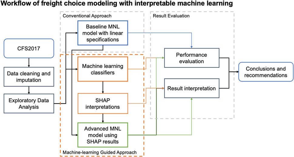
FIGURE 1. Workflow of freight choice modeling with interpretable machine learning methods.

2.1 Data cleaning and imputation

In this study, the shipments originating from and/or attracting to the greater Austin region, including Austin-Round Rock (CFS code 48-12420), San Antonio-New Braunfels (CFS code 48-41700), and the remainder of Texas (CFS code 48-99999), are selected from CFS 2017 (U.S. Census Bureau, 2020) as the primary data source to estimate the freight mode choice model. A shipment in CFS2017 is defined as a single movement of goods, commodities, or products from an establishment to a single customer or another establishment owned or operated by the same company as the originating establishment. Each shipment record includes detailed shipment characteristics, such as shipment weights, distance, Standard Classification of Transported Goods (SCTG) commodity types, and industry code (NAICS) of the shippers. All these characteristics are essential drivers of freight mode choice decision-making, as discussed in the Introduction. A total of 103,877 shipments are reported in CFS 2017, providing a modal picture of disaggregated national freight flows and representing the only publicly available source of multimodal commodity flow data (Bureau of Transportation Statistics et al., 2020).

2.1.1 Data cleaning and pre-processing

The raw Austin-region dataset consists of 253,810 shipments using 15 transportation modes. Several data-cleaning measures are undertaken before model development to ensure the data quality and practicality of model estimation. First, the modes representing less than 0.3% of the sample are dropped due to their low market share. Therefore, modes such as waterways and pipelines are excluded. Samples missing critical information, such as shipment weights and commodity types, are also excluded. In addition, the data removal rules described by Stinson et al. (2017) are applied to remove potentially erroneous records, such as air shipments above 15,000 lbs. or rail shipments less than 1,500 lbs. Finally, international shipments are excluded due to gaps in generating factors (e.g., travel time and cost) to account for their shipping characteristics. The remaining shipments are categorized into five modes, including 1) for-hire truck, 2) private truck, 3) intermodal rail (both rail and InterModal truck + rail eXchange [IMX]), 4) air, and 5) parcel. The two rail-based modes are combined into one rail intermodal (rail/IMX) mode as each of them separately does not have a sufficiently large sample size and may lead to difficulty in estimation if modeled separately. The final sample size and mode split are summarized in Figure 2. The cleaned Austin data contain 247,073 shipments, with 2.6% of samples removed due to the above-described data cleaning steps.

FIGURE 2

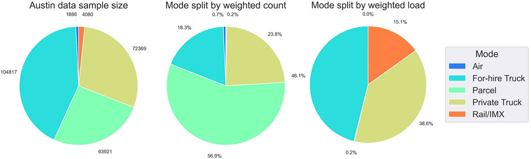
FIGURE 2. Summary of sample size and mode split in cleaned Austin CFS data.

2.1.2 Explanatory variable selection and imputation

The 2017 CFS dataset provides key shipment characteristics to be used as explanatory variables in mode choice models. The variables included for the model estimation, as well as their summary statistics by freight mode (weighted by CFS scaling factors), are provided in Table 1 and Figure 3. Regarding shipment distance, private trucks are typically used for short-distance shipments, while longer-distance shipments are often made by rail, parcel, and air. Regarding shipment weights, trucks (private and for-hire) are used more often for shipments greater than 150 lbs. The share of freight carried by trucks declines and shifts to rail when shipment weights reach 30,000 lbs. Finally, both trucks and rail are more often used for shipping lower-value-density commodities, while parcel and air are more often used for higher-value goods. All these factors play essential roles in freight mode decision-making and are included in the mode choice model.

TABLE 1

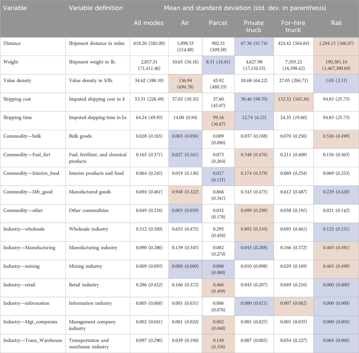
TABLE 1. Summary statistics for selected explanatory variables (blue–lowest, red–highest).

FIGURE 3

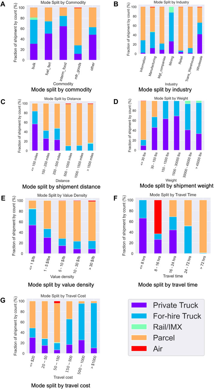
FIGURE 3. Summary of freight mode split by selected explanatory variables: (A) commodity type, (B) industry type, (C) shipment distance, (D) shipment weight, (E) value density, (F) travel time, and (G) travel cost.

Several categorical variables are derived to reduce the dimensionality of the input features, including the commodity type and industry type. The 41 commodity types in CFS2017 are grouped into five categories based on shared characteristics: 1) bulk commodities; 2) interim products and food; 3) fuels, fertilizers, and other chemical products; 4) manufactured goods; and 5) other unclassifiable commodities. The commodity type categorizations are presented in Supplementary Table SA1. As shown in Figure 3, those commodity groups have different preferences for freight mode, with trucks and rail mainly adopted for bulk goods and parcel modes primarily used for manufactured goods. Regarding industry type, the 2-digit North American Industry Classification System (NAICS) codes of the shippers are used to represent broader industry types. As shown in Figure 3, the mining industry relies heavily on truck and rail/IMX modes, while retail, management, and information industries prefer the parcel mode. The transportation/warehouse industry has a high parcel shipment share as CFS2017 only surveyed freight trucking and warehousing establishments in this category (Bureau of Transportation Statistics et al., 2020). Those establishments mostly perform local pickup and delivery, sorting and terminal operations, and line haul, leading to substantial parcel shipments.

In addition to the attributes obtained directly from CFS 2017, two level-of-service variables, specifically shipping costs and shipping time, are used in the mode choice model. These variables are estimated based on methods described by Stinson et al. (2017) for truck and rail and by Keya (2016) for air and parcel (as the former study combined air and parcel into a single mode). The detailed parameters of shipping time and cost imputation are provided in Supplementary Table SA2. As those variables are imputed using empirical values and may not capture shipment-level variation, they are included as generic variables in model estimation. The nonlinear relationships for mode preferences by shipping time and costs are not explicitly studied in this work. Shipping time is composed of in-vehicle travel time (IVTT) plus delays/idling time for most modes except parcel. The IVTT is estimated using distance and mode-specific average speed, as presented in Eq. 1. The delay/idling times are estimated using values from empirical studies.

$t=t_0+\frac{d}{v}(1)$

• $t$ is total shipping time;

• $t_0$ is delay time;

• $d$ is the distance in miles;

• $v$ is the mode average speed in mph.

For parcel mode, Keya (2016) calculated that the shares of shipping speeds of overnight (1-day), express (3-day), and ground service (5-day) were 18%, 9%, and 73%, respectively, based on FedEx data. Shipments are randomly assigned to the three options using this time distribution. According to Figure 3, private trucks and air are primarily used for shorter trips within the day, while for-hire trucks, rail, and parcel are more often used for multi-day shipments.

The shipping cost for all modes other than parcel is composed of a minimum charge and an elastic charge based on the shipping rate and shipment quantify, as shown in Eq. 2. The minimum charge and shipping rate can vary by shipment characteristics, such as weight and distance.

$C=\mathit{max}\left(c_0,c_1\ast x\right)(2)$

• $C$ is the total shipping cost;

• $c_0$ is the minimum charge;

• $c_1$ is the shipping rate;

• $x$ is the quantity of shipment (weight for truck/rail or weight*distance for air/parcel).

For the parcel mode, an exponential function is applied to generate the shipment cost based on parcel weight. Based on Figure 3, shipping costs for parcel modes are generally cheaper, while for-hire trucks are often more expensive.

2.2 Conventional approach of the freight mode choice

Conventional discrete choice models are based on random utility theory, which assumes decision-makers select the alternative with the highest utility (Ben-Akiva and Lerman, 1985). Those utilities are not known with certainty and are treated as random variables. In the case of freight mode choice, using the MNL approach as presented in Eq. 3, the utility $U_{ik}$ of choosing mode $k$ for shipment $i$ takes the following form:

$U_{ik}=v_{ik}+{\epsilon }_{ik}={{\alpha }_k+\beta }_k{X}_i+{\gamma }_k{Y}_{ik}+\delta Z_{ik}+{\epsilon }_{ik}(3)$

• $U_{ik}$ is the utility derived from selecting mode $k$ for shipment $i$;

• $v_{ik}$ is the systematic component of the utility;

• ${\epsilon }_{ik}$ is the unobserved error term, assumed to follow the Gumbel distribution;

• ${\alpha }_k$ is the alternative-specific constant vector;

• $X_i$ is the vector of shipment-level factors, including the commodity group, shipper industry group, shipment weight, and value density;

• ${\beta }_k$ is the alternative-specific coefficient vector associated with shipment-level attributes;

• $Y_{ik}$ is the vector of joint shipment-level and alternative-specific factors, notably shipment distance (routed distances for truck and rail and great circle distances for parcel and air);

• ${\gamma }_k$ is the vector of shipment distance coefficients;

• $Z_{ik}$ is the vector of imputed level-of-service factors, including travel time and shipping costs;

• $\delta$ is the generic coefficient vector for travel time and shipping costs;

The probability $p_{ik}$ of choosing mode $k$ from a set of $K_i$ available alternatives for shipment $i$ can then be specified, as shown in Eq. 4.

$p_{ik}=\frac{\mathit{exp}\left(v_{ik}\right)}{{\displaystyle \sum _{k\in K_i}}\mathit{exp}\left(v_{ik}\right)}.(4)$

Mode availability constraints are imposed on individual shipments to generate the available choice set, $K_i$, based on the following rules, as suggested by CFS2017 data:

• Parcel mode is only available to shipments below 150 lbs.

• Air mode is only available to shipments below 410 US tons.

• Private truck mode is only available to shipments within 500 miles.

2.3 Machine learning guided approach

The second pathway to estimate the freight mode choice model is using the insights from ML classifiers to improve the specifications in MNL models. This approach provides broader benefits beyond improving the model prediction accuracy demonstrated in prior studies (Zhao et al., 2020; Uddin et al., 2021; Javadinasr et al., 2023). It also offers a practical way of visualizing and understanding the complex relationships between various factors and behavioral outcomes and capturing those complex relationships into the conventional logit model structure.

2.3.1 Machine learning method selection and estimation

In this study, three tree-based ML methods are selected for the freight mode choice estimation due to their 1) suitability for resolving nonlinear relationships observed in high-dimensional data with high accuracy and 2) seamless connection with the SHAP TreeExplainer (Lundberg et al., 2020) to ensure interpretability. Tree-based methods partition the factor space into a set of rectangles and then fit a simple model (like a constant) in each one (Hastie et al., 2009). There are three major advantages of the tree-based methods in the context of modeling freight mode choice: 1) tree-based methods have advantages in handling mixed data types, missing values, and outliers, which are known issues within CFS data (Bureau of Transportation Statistics et al., 2020); 2) tree-based methods are computationally efficient and do not require intensive computational resources; and 3) when boosted or ensembled, tree-based methods can fit high-dimensional data with high accuracy. In previous applications, tree-based models consistently outperformed standard deep learning models on tabular-style datasets where features are individually meaningful and do not have strong multi-scale temporal or spatial structures (Lundberg et al., 2020). They also outperform many other ML classifiers and achieve similar accuracy to deep neural networks in the area of travel behavior (Wang et al., 2021). Therefore, they are promising in predicting mode choice with the CFS2017 data. Specifically, the following tree-based ML models are selected for this study:

Random forest (RF): RF (Breiman, 2001) is a substantial modification of bagging that builds a large collection of de-correlated trees and then averages them. RF models often perform similarly to boosting methods, and they are simpler to train and tune. In a previous benchmark effort comparing the performance of various ML and discrete choice models in travel behavior studies, the RF method was the most computationally efficient, thus balancing between prediction and computation (Wang et al., 2021).

Boosting trees: The motivation for boosting was a procedure that combines the outputs of many “weak” classifiers to produce a powerful “committee” by constructing an ensemble predictor using gradient descent in a functional space (Hastie et al., 2009; Prokhorenkova et al., 2017). There are many implementations of boosting tree classifiers, such as XGBoost, pGBRT, LightGBM, and CatBoost (Chen and Guestrin, 2016; Prokhorenkova et al., 2017). In this study, two boosting tree methods are selected due to their scalability for large datasets and demonstrated model accuracy in prior studies.

• XGBoost: XGBoost is a scalable ML system for tree boosting that is computationally efficient, provides scalable solutions to many complex problems, and is suitable for handling sparse data (Chen and Guestrin, 2016). Those advantages are particularly relevant for the freight mode choice model, especially given that most shipments are heavily skewed toward regional travel, manufactured products, and a subset of industries, as indicated in Table 1.

• CatBoost: CatBoost is another tree-based boosting method that implements an ordered boosting algorithm for processing categorical data (Prokhorenkova et al., 2017). With such an implementation, CatBoost addresses the “prediction shift” of other boosting methods, in which the distribution of prediction shifts from training data to testing data. CatBoost often outperforms other boosting methods in modeling categorical data and thus is selected for estimating the freight mode choice model.

The selected ML methods are trained and tested in Python, using input factors described in Table 1. A stratified sampling is used to generate the 80%/20% training/testing split by mode to include sufficient observations within each mode. The hyperparameter selection and cross-validation are performed using the “HalvingGridSearchCV” function from Python’s “scikit-learn” package (Pedregosa et al., 2011) on training data. Essential model hyperparameters, such as learning rate, regularization terms, and tree size, are selected to provide the highest cross-validation accuracy. Model performances are demonstrated using the out-of-sample testing data.

2.3.2 Model interpretation and enhancing specification using SHAP TreeExplainer

In addition to accuracy, these ML methods are also expected to be interpretable and explain how the model uses the input features to make predictions (Lundberg et al., 2017). While the tree-based methods provide feature importance to rank the global contributions of input factors on the output, they often lack a way to provide local explanations that show the direction of impacts of input factors on individual predictions or interactions among input factors. To address this, the SHAP TreeExplainer is introduced to provide a local explanation for tree-based models (Lundberg et al., 2020). It facilitates the exact computation of optimal local explanations for tree-based models, captures factor interaction, and provides a set of visualization tools to understand global model structure based on local explanations. In TreeExplainer, Shapley values (the attributions of output to factors) are computed by introducing each factor into a conditional expectation function, $f_x$, of the output, as presented in Eq. 5.

$f_x=f_x\left(S\right)\approx E\left[f\left(x\right)|x_S\right](5)$

• $f\left(.\right)$ is the estimated model;

• $x$ is a specific input;

• $S$ is the subset of factors (or independent variables).

Using the conditional expectation functions in Eq. 5, the Shapley values in TreeExplainer are defined in Eq. 6.

${\varphi }_i\left(f,x\right)={\displaystyle \sum _{S\subseteq N\backslash \left\{i\right\}}}\frac{\left|S\right|!\left(M-\left|S\right|-1\right)!}{M!}\left[f_x\left(S\cup \left\{i\right\}\right)-f_x\left(S\right)\right](6)$

• ${\varphi }_i\left(f,x\right)$ is the attribution (or Shapley value) of the $i$ ^th factor to tree-based model $f$ among input $x$;

• $N$ is the set of all factor ordering;

• $S$ is the subset of all factors that do not include factor $i$;

• $M$ is the number of input factors for the model.

After calculating the SHAP values for ML classification models, the attribution of each factor toward the preference of each mode, ${\varphi }_i\left(f,x\right)$, can be generated for each observation to understand the local impact of these factors. A series of SHAP visualization tools is demonstrated in Figure 4 using SHAP values from the CatBoost model to illustrate how to interpret ML outcomes using TreeExplainer and leverage those insights for MNL specifications. First, an example of the SHAP interpretation of a single observation is provided in Figure 4A, which illustrates the SHAP values for a single shipment and selection of a single mode. The model output of the single shipment, in this case, the log odds of choosing private truck, is captured in the blue line. The expected log odds corresponding to values on the x-axis are generated after introducing each factor, and the final values after including all factors are color-coded on the line. Each row represents how individual factors shift the model output to its final values; for example, travel time and distance decrease the log odds of choosing private truck, while shipment weight increases the log odds. The value in parentheses annotates the current values of each factor; for example, the distance for this shipment is approximately 900 miles. Overall, most factors contribute negatively to the log odds of choosing private trucks, with travel time having the largest negative impact. Some factors, such as all the industry indicators, do not affect the preferences for selecting private trucks in this case. After performing a logit conversion of the model output and decomposing factor contributions by the probability of choosing private truck in Figure 4B, the trends are even clearer. Introducing travel time to the model led to the expected probability of choosing private truck shift from 0.6 to 0.1, while distance, travel cost, and value density also contributed negatively but to a lesser extent. In summary, the SHAP TreeExplainer helps define how the combination of input factors contributes to individual observations and can help users understand the local effects of various factors in estimating results.

FIGURE 4

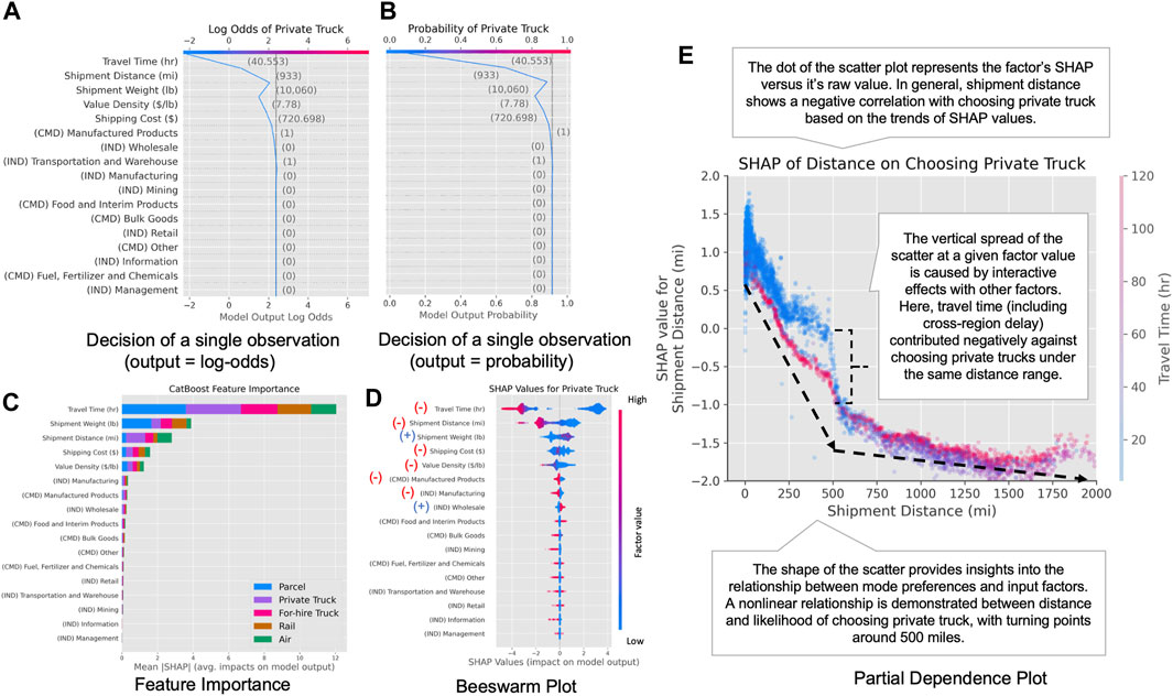
FIGURE 4. Illustration of SHAP TreeExplainer interpretations, including: (A) SHAP interpretation of single observation using log-odds, (B) SHAP interpretation of single observation using probability, (C) global feature importance of all modes, (D) beeswarm plot of a single mode, and (E) dependence plot of a selected factor for a single mode.

The SHAP interpretations of each observation and mode must be assembled to generate the final insights to support the specification of the MNL model, which captures the global trends of all observations. In addition, the SHAP value is calculated using output log odds of choosing each mode from the ML model, which provides a direct connection between the SHAP interpretations from the ML model and the functional forms of mode utilities in the MNL model. Three sets of summary results are provided to show the relationship between the predicted outcomes and input factors (Lundberg et al., 2020) and can be used to guide the development of MNL specifications:

2.3.2.1 Global measure of feature importance for variable selection

Global feature importance is generated by averaging the absolute SHAP values across the entire dataset, as illustrated in Figure 4C. It indicates the global importance of all input factors and is often used as a reference for variable selection. The variables labeled with “CMD” are commodity types, while variables labeled with “IND” are industry indicators. The factors ranked at the top of the figure, such as travel time, distance, and cost, have substantial impacts on mode selection and should be kept in MNL specifications. The lower-ranked factors with low feature importance, such as management and information industry, have negligible impacts on the results and can be dropped from model specifications.

2.3.2.2 One-dimensional scatter plots (or beeswarm plots) for identifying the direction of impacts

The beeswarm plots provide both the magnitude and prevalence of a factor’s effect for each output class, as illustrated in Figure 4D. Each point represents the SHAP values of a single factor toward each mode within a single observation, and the vertical spread of each swarm represents the density of the points. The direction of such effects can also be revealed by adding color that reflects the raw factor values. The directions of impacts are labeled for the top eight influential factors based on the sign of the SHAP values under various factor values. For example, lower travel time tends to have positive SHAP values on log odds of private trucks, suggesting a negative correlation between travel time and preference toward private trucks. The beeswarm plots can be used to validate the direction of impacts in MNL estimations and to identify potential mixed impacts if no clear directions are identified in the plots.

2.3.2.3 Dependence plots of individual features for nonlinearity identification

Plotting the factor’s values on the x-axis and the factor’s SHAP values on the y-axis for all observations produces a SHAP dependence plot that shows how much a selected factor impacts the prediction of a candidate mode, as illustrated in Figure 4E. The interactive effects of several factors can also be revealed by color-coding each dot with a secondary factor. The direction of the scatter shows the direction of impacts for selected factors, with a downward trend indicating the negative impacts of this factor on selecting the specific modes and vice versa. The slope of the scatterplots indicates whether potential nonlinearity is observed for selected factors on choosing this mode, and intervals of factor values with different slopes suggest that potentially heterogeneous effects are being captured by the MNL model. The vertical spreads under fixed factor values indicate the degree of interactive effects associated with this factor value, color-coded by factors with the highest interactive effects. The dependence plots are useful in determining nonlinear functional forms of mode-specific variables in MNL specifications, and the turning points of SHAP dependence plots can be used to define the nonlinear bins in an MNL model. The color code from SHAP can also inform potential interactive factors to be included within the MNL specifications.

In summary, the insights from the SHAP TreeExplainer can be used to enhance the specifications of the MNL model. The potential new specifications may include 1) selecting factors based on feature importance, 2) generating nonlinear specifications, such as using binary variables with binning/turning points identified from SHAP dependence plots, and 3) adding interaction terms. Not all the observed relationships can be estimated in the MNL model, as it has a much longer run time and becomes computationally impossible to fit with large sample sizes, high input dimensions, or simulation-based estimation (Wang et al., 2021).

Finally, the performances of each model (both MNL and ML) are evaluated using several accuracy measures on the out-of-sample testing dataset, including overall accuracy, precision, recall, and F1-score. The accuracy measures can be combined for all modes either through the flat average of mode-specific measures (macro average) or weighted by sample size in each mode (weighted average). The detailed formulation of each performance metric can be found in Supplementary Appendix B. In addition, result interpretations from best-performing ML and MNL models are also compared against each other to investigate if both models suggest similar mode preferences with respect to key influential factors. The directions of impacts from both sets of models are compared, together with findings from empirical studies, to examine if a correlation derived from ML is supported by causal relationships defined through the econometric approach and if convergences can be drawn from two distinct approaches.

3 Results

The methodology described above is implemented in the Austin region to develop MNL and ML models and provide insights into freight mode choice decision-making. Specifically, a baseline MNL model (“bMNL”) is estimated using the conventional approach described in Section 2.2, while an advanced MNL (“aMNL”) model is estimated with ML-guided improvements to the baseline as described in Section 2.3. This section compares the performance of the MNL and ML models to evaluate the accuracy of different approaches. Next, results from the SHAP TreeExplainer are demonstrated with the best-performing ML model to investigate the relationships between various factors and freight mode choice. Finally, the bMNL and aMNL results are compared to the insights from the SHAP interpretation. The conclusions and recommendations are drawn based on the SHAP results and the aMNL estimations.

3.1 Performance measures

The performance measures of all models are illustrated in Figure 5, with performance metrics generated from out-of-sample testing data. Regarding overall classification accuracy, RF and CatBoost have the highest accuracy, followed by XGBoost, and the tree-based models outperform the MNL models. The aMNL model has higher accuracy than the bMNL model, with additional parameters capturing nonlinear relationships. Regarding detailed accuracy measures such as precision, recall, and F1-score, MNL models generally have lower accuracy than ML models. The aMNL model provides a better balance between precision and recall (as they move in opposite directions) than the bMNL model, leading to slightly higher F1-scores in aggregate. Finally, regarding accuracy by modes, ML methods generate accurate predictions for all modes, while the accuracies of the two truck modes are slightly lower (as they share great similarities and existing factors may be insufficient to distinguish them). Compared to ML, MNL models have larger prediction errors with respect to air and rail/IMX modes, potentially due to their low sample size. The aMNL model helps improve F1-scores for for-hire truck and rail compared to the bMNL model, while F1-scores for other modes do not change. In general, ML models outperform MNL models in all performance measures, but partially including the nonlinear relationship in the MNL specifications helps increase the accuracy of MNL models.

FIGURE 5

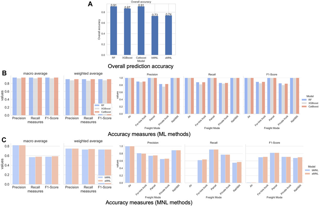
FIGURE 5. Performance comparison of all models on testing data, including (A) overall prediction accuracy, (B) accuracy measures of ML methods, and (C) accuracy measures of MNL methods.

3.2 Machine learning model performance and interpretation

In this study, SHAP interpretations are generated from the CatBoost model for a close examination of the results. Among the three ML models, CatBoost demonstrates the best performance (and is similar to RF) and supports the exact estimation of SHAP values, while SHAP values of the RF model can only be approximated due to the high computational burden. The outputs of CatBoost provide log odds for each output class (freight mode in this study), and SHAP values are estimated for each mode to demonstrate the attribution of factors to expected log odds for all five freight modes (regardless of mode availability). Positive SHAP values indicate increases in the log odds of the predicted freight mode or preferences toward this mode and vice versa. First, the global feature importance using mean SHAP values is shown in Figure 4C, color-coded by mode to show the attribution of those factors to each freight mode. Travel time, cost, shipment weight, distance, and value density are the top five factors that affect the freight mode choice. Industries such as management, information, and mining have negligible impacts on freight mode choice, potentially due to their low presence in the region, as indicated in Table 1.

Next, the beeswarm plots in Figure 6 demonstrate the importance ranking of input factors and the direction of impacts toward each freight mode. The factors on the top with a wider range of SHAP values are the most important factors influencing a selected freight mode; the density of the dots shows the number of observations, and the color of the dot shows in which direction the factor drives the mode choice. For for-hire trucks, used as the base alternative in the MNL model, higher shipment weight and distance increase the likelihood of choosing for-hire truck, while higher value density decreases the preferences toward this mode. The shipment distance has the opposite impacts on private versus for-hire trucks, while impacts of other top influential variables remain similar between the two truck modes. Rail mode shows great similarity to for-hire trucks in terms of major factors and directions of impact, except that travel time is often positively correlated with rail due to its longer delays. Air and parcel modes show different use cases from truck and rail and are more likely to be used for high-value and light-weight goods. Most industry and commodity variables show relatively small impacts on the mode selection. A few notable findings include shipments containing manufactured goods or from manufacturing industries exhibiting a negative preference towards private trucks and a positive preference for air. All of these relationships are aligned with observed trends from Figure 3. Finally, the beeswarm plots suggest some nonlinear relationships between factors and mode selection, especially when asymmetrical positive versus negative SHAP values are observed. For example, in the case of rail mode, the higher shipment weight segment has a long tail of positive SHAP values, while the lower weight segment has negative SHAP values close to 0, suggesting the higher weight segment has a more profound impact on choosing rail.

FIGURE 6

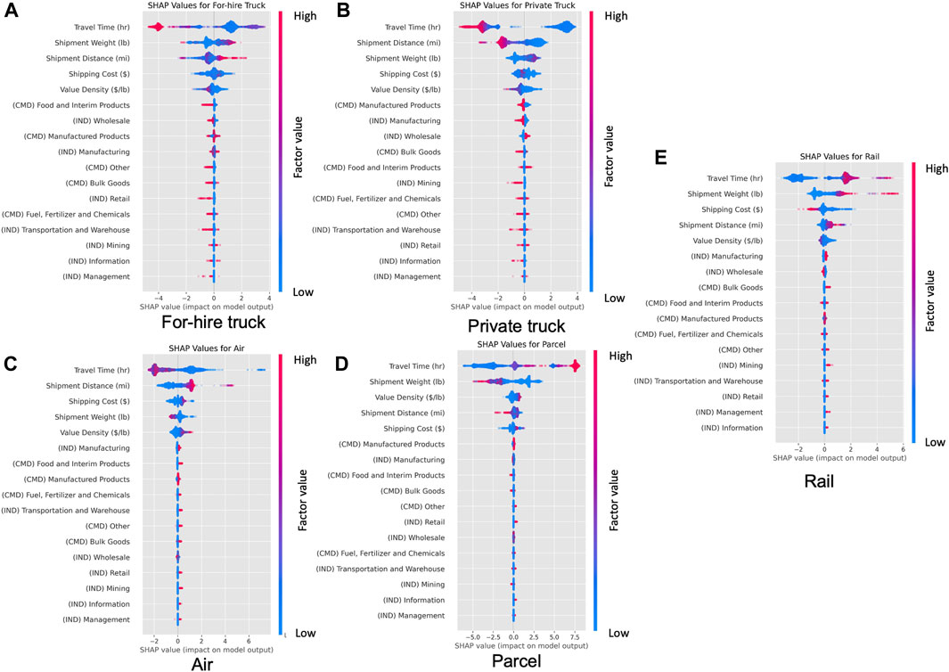
FIGURE 6. Local feature importance of input factors by mode, including (A) for-hire truck, (B) private truck, (C) air, (D) parcel, and (E) rail.

The dependence plots in Figure 7 provide a clear view of intricate relationships between each freight mode and top influential continuous factors (excluding travel time and cost as they are imputed and not individual-specific). The shapes of the curves show the relationship between input factors and predicted log odds of freight mode. The vertical spread at a fixed factor level indicates the degree of interactive effects the selected factor has with other factors toward freight mode selection. Some plots are zoomed in to show the location of turning points (e.g., air and parcel modes are mostly used for small shipments, so the weight ranges are truncated). For distance, weight, and value density, almost all the relationships demonstrated are nonlinear, and some are non-monotonic. In general, when distance increases, the likelihood of private trucks decreases, while the likelihood of for-hire trucks and air increases. Rail and parcel modes show some mixed and non-monotonic changes. However, after a 500-mile range, the SHAP curves turn flat for almost all modes, and the increment of distance no longer causes a major shift in mode preferences. For shipment weight, the likelihood of choosing truck and rail increases with higher weights, while the likelihood of parcel and air decreases. For all freight modes, there appears to be a weight threshold (e.g., 150 lbs. for air), and the levels of impact almost stay constant after that threshold. For value density, the directions of impacts under low-value density (≤ $5/lb.) are mixed, especially for for-hire trucks and rail. The level of impacts almost remains constant after $25/lb., and additional value density does not seem to bring substantial changes to the mode preferences.

FIGURE 7

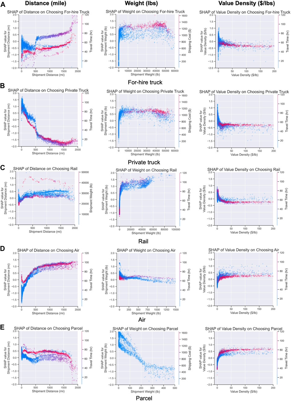
FIGURE 7. Dependence plots for selected factors and all modes, including (A) for-hire truck, (B) private truck, (C) rail, (D) air, and (E) parcel.

Some interesting interactive effects are observed in Figure 7. For example, for private trucks, the SHAP values under the low distance range with longer travel time (perhaps long-haul trips across the region) declined faster than the curve under short travel time. This suggests that private trucks are less preferred if the trips are external to the region and face more potential delays. A similar relationship is also found in for-hire trucks as longer travel time with overnight delay will discourage the use of for-hire trucks over the same distance range. For the two truck modes, the impacts from value density changes are much less under the long travel time cases, potentially due to elevated travel costs in those cases offsetting the attributions of value density. Similarly, for air mode, the SHAP values of value density are lower under the longer travel time cases, suggesting that the longer travel time lowers the likelihood for air even if the value density is high. Finally, for air mode, the SHAP curve of weight is also flat under the long travel time case, and the influence from weight is less significant when travel time is high. Those interactive effects may result from how the travel time and costs are imputed and their high correlation with other factors. Nevertheless, as travel time and costs capture major differences in modal service quality and have potential impacts on mode choice, they should be collected in future survey efforts to advance the modeling practice.

3.3 MNL model results and comparisons of interpretation

Without considering insights from SHAP, the bMNL model is estimated using all the factors combined with necessary binning to prevent collinearity of variables (e.g., the weight bins are adopted to prevent collinearity with shipping costs). The estimation results are provided in Table 2. Overall, the bMNL model has a reasonable performance with an adjusted ${\rho }^2=0.567$. Most coefficients are aligned with the SHAP values in terms of directions of impacts, with some nuances to interpretation needed as MNL models capture relative preferences compared to the omitted alternative while the SHAP values reflect the absolute preferences toward all individual modes. For example, although long distance generally increases the preference for rail, it is still less preferred than for-hire truck and thus has a negative coefficient in the bMNL model. In general, the results from MNL models do not capture the intricate relationship demonstrated in Figure 7. For example, value density has non-monotonic and substantial impacts on rail, while the bMNL model does not generate a significant result due to such a mixed effect. For parcel, the bMNL model fails to generate a significant coefficient for value density despite the strong impacts indicated in Figure 7. Rather, several industry indicators, such as management and information, have significant estimation of coefficients at 95% confidence level. Those low-impact factors may be correlated with more influential factors, thus absorbing their effects, and the estimated coefficients may be arbitrary and can mislead the result interpretation.

TABLE 2

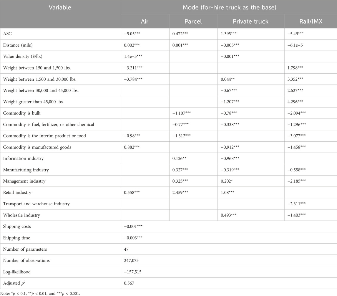
TABLE 2. Baseline MNL mode choice model estimation results for Austin, TX.

Next, the insights from the SHAP interpretation are incorporated to revise the specifications of the bMNL model to improve its performance, and the estimation results of the aMNL model are provided in Table 3. Overall, with four more parameters estimated, the aMNL model achieves higher adjusted ${\rho }^2=0.576$ than the bMNL model. The likelihood ratio test also suggests that the aMNL model is significantly better than the bMNL model at the 99% confidence level. The SHAP results help remove nine low-impact factors, such as most industry indicators for parcel and rail. In addition, binned specifications are introduced for distance and value density for most modes, which helps reveal significant relationships between those modes and explanatory factors. In general, the directions of impacts for most variables are aligned with SHAP interpretations from the CatBoost model, as illustrated in Figures 6, 7. There are a few exceptions where trends are visible in Figure 7 but are not found to be significant in aMNL models, such as long distance for air, potentially due to lack of observations and impacts from confounding factors.

TABLE 3

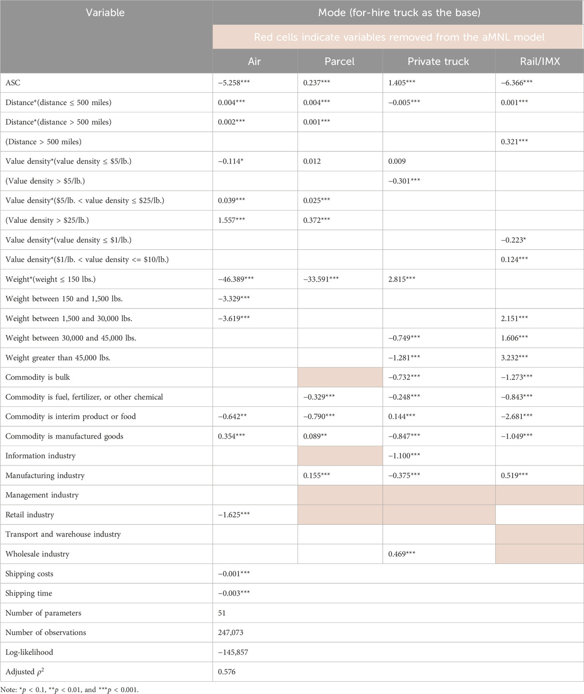
TABLE 3. Advanced Austin-region MNL mode choice model using SHAP results.

For shipping distance, after using a piecewise linear function for parcel in the aMNL model, the linear portion under the low-distance range shows a higher coefficient than the bMNL model, indicating more substantial impacts of distance during this range for choosing parcel over for-hire truck. In addition, after applying a binned approach for rail distance, the aMNL model demonstrates a significant positive impact of distance on rail within the 500-mile range, which is aligned with the interpretations from CatBoost in Figure 7 and similar to findings from a prior study (Pourabdollahi et al., 2013). The disutility of distance in the aMNL model for private trucks over for-hire trucks remains unchanged compared to the bMNL model and consistent with SHAP interpretations and findings from the prior study that uses CFS data and the same truck mode definitions (private versus for-hire trucks) (Keya et al., 2019).

For value density, after introducing bins into the specification, both parcel and rail have significant coefficients estimated in the aMNL model. For parcel, although value density already shows some positive impacts in choosing parcel under a low-value-density range, the coefficient of value density within $5–25/lbs. is even larger than values below $5/lbs. After $25/lb., a positive constant coefficient is estimated, and adding more value density does not further increase the likelihood of parcel. The increasing likelihood of choosing parcel and air under higher-value density is also aligned with findings from prior studies, where modes like air that carry smaller shipments are preferred for high-valued goods (de Jong and Ben-Akiva, 2007; Pourabdollahi et al., 2013). For rail, value density negatively impacts rail preference if lower than $1/lb., but the impacts become positive if value density is between $1–$10/lb., which is aligned with the mixed influences in Figure 7. In prior studies, it has been shown that preference for rail over trucks generally decreases with a higher value of goods (Jensen et al., 2019), while results in this study provide a more complex response to value density for rail mode. The coefficient for private truck only shows a constant negative impact under the high-value density case.

For shipment weight, while the original weight bin definitions are kept, a linear weight specification is applied to the lowest weight bin to capture greater sensitivity to weight within that range. In general, those weight bins capture major turning points, as indicated in Figure 7, with estimated coefficients remaining similar. Incorporating weight multipliers helps explain the strong negative impacts of weight on air and parcel modes and the positive impact on private trucks within the low-weight range. While numerous prior studies have performed joint modeling of shipment size bin and mode choice (de Jong and Ben-Akiva, 2007; Pourabdollahi et al., 2013; Stinson et al., 2017; Keya et al., 2019), the results from this study suggest the preferences of modes (especially air and parcel) are highly sensitive to weight, and more disaggregated specification of shipment size for these modes is potentially needed. Finally, the positive impact of weight on choosing rail over truck has been demonstrated in prior studies (Samimi et al., 2011), while the results from this study further demonstrate the more substantial impacts over the higher weight range.

In general, the aMNL model provides more explanatory power for factors that displayed nonlinear relationships with mode choice than the bMNL model and removes the factors that may mislead model interpretation. However, not all the SHAP relationships can be successfully implemented in an MNL model, potentially due to 1) lack of observations for some cases causing singularity in model estimation (e.g., long distance interacted with multi-day travel of private trucks is omitted due to lack of sample); 2) collinearity among variables causing counterintuitive results for key factors. In this study, the maximum number of parameters with meaningful interpretation was retained in the aMNL model, capturing some of the most important nonlinear relationships indicated by SHAP interpretations.

4 Conclusion and discussions

In this study, we estimate a logit-based freight mode choice model using the CFS2017 survey, informed by results from state-of-the-art ML models and interpretable ML methods. The influential factors and their relationship with individual freight modes are identified using ML and SHAP TreeExplainer and applied to the MNL model specification to improve its performance. The workflow is demonstrated using a case study for Austin, Texas. In general, ML models outperform MNL models in both overall accuracy and mode-specific accuracy measures. By applying the CatBoost model and SHAP TreeExplainer, we evaluated the relationship between the predicted outcomes and input features and then identified factors like travel time, cost, shipment distance, weight, and value density as the most influential. In contrast, industries such as management, information, and mining show negligible impacts on mode selection. Nonlinear relationships are observed for shipment distance, weight, and value densities across all modes. Additionally, value densities display mixed, non-monotonic impacts on the selection of both rail and for-hire trucks. Upon applying some of those insights to refine the MNL specifications, the MNL model’s interpretability and accuracy surpass that of the baseline model. Moreover, the advanced MNL model reveals significant and complex relationships that are hidden in the baseline model, such as the impact of value density on the selection of rail and parcel. The directions of impacts yielded by the aMNL and CatBoost results are often aligned with findings from empirical studies and help reveal more intricate relationships between some factors and mode preferences.

4.1 Contributions to freight mode choice applications

The methodology and results from this study can help advance freight mode choice applications in several ways. First, the comparison of result interpretations in this study demonstrates some convergence between MNL and ML results because the insights from the two approaches are generally aligned with each other. Some of the nuanced trends from ML methods may not lead to significant parameter estimates in an MNL model, but the major trends/behavior preferences can be captured in an MNL model and supported by a more theory-based approach. Although ML methods cannot be directly used to demonstrate causal relationships, the joint insights from ML and ML-guided MNL approaches suggest ML methods are still useful in identifying potential hypotheses for testing in econometric approaches. Second, ML methods combined with SHAP interpretations can also help prioritize highly influential factors and vice versa. This approach enhances the refinement of MNL models, helps prevent arbitrary variable selection, and reduces the risk of incorrect interpretation caused by confounding factors. It also saves the time and effort needed to develop MNL specifications, which is pertinent to users and practitioners who operate within a limited timeframe and computational resources, as training discrete choice models on a large dataset can be computationally challenging (Wang et al., 2021). Furthermore, the ML methods and SHAP interpretations approach serve as more practical and intuitive methods for data exploration, in addition to the conventional cross-tabulation approach, and are especially powerful in revealing individual-level heterogeneity of preference instead of only showing generalized trends (Lundberg et al., 2020). Finally, the technical workflow demonstrated in this paper could also support freight model choice modeling in other regions or countries with analogous data, thereby advancing the state of the practice in this domain.

4.2 Policy implications

The findings from this study can help inform freight-related policymaking and deepen the understanding of how potential policies might influence mode shift and subsequent transportation externalities (e.g., congestion, energy, or emissions) in specific contexts. First, by including nonlinear relationships in the model specification and achieving better accuracy, the MNL model becomes more helpful in revealing complicated trade-offs between mode selection and influential factors. For example, with a nonlinear relationship between weight and air/parcel, the bundling or consolidation of packages may have greater impacts on mode shift from air/parcel to trucks in lower-weight versus higher-weight packages. On the other hand, policies targeting very long distance, heavy shipments, or high-valued goods may be less effective as the preferences toward each mode are more stable in those ranges, and additional changes of those factors do not lead to sizeable mode shifts. By further integrating the freight model choice model derived in this study with traffic simulation tools (Spurlock et al., 2024), the system-level impacts of congestion mitigation, energy efficiency, and environmental impact policies can be further investigated at the regional level. Finally, from a theoretical perspective, the empirical findings and domain knowledge derived from various contexts and datasets can serve as a priori, whereas the findings from interpretable ML methods can provide additional evidence or insights into the trends from a specific dataset as posteriori. Both sets of insights and findings are valuable for developing a comprehensive understanding of the mechanism of freight mode choice and supporting MNL model estimation, interpretation, and amendment.

4.3 Future research directions

The findings and insights drawn from this study are constrained by the limited number of factors available from the survey data, with potential impacts of unobserved factors to be revealed through future work. Additional influential factors, such as shipping reliability and quality of service (Holguín-Veras et al., 2021), should be accounted for in the model if available from more recent data sources. In addition, the current analysis is based on the 2017 data, and the prevalence of freight modes is constantly changing, especially due to the COVID-19 disruptions on road, air, and rail freight transportation (Borca et al., 2021; Khan et al., 2022). The freight mode choice model will be revisited and updated if more recent data and additional attributes become available.

The existing methodology can also be further enhanced to achieve better modeling performance and advance our understanding of freight mode choice behavior. Potential future work includes 1) improving the travel time and cost estimation by incorporating local transportation data, either observed or modeled, to enhance the accuracy of the model and capture the local congestion patterns; 2) exploring other high-performance ML models, such as deep neural network and the ensemble of several ML classifiers, to further improve the model accuracy and reveal additional complex relationships potentially not yet discovered in current models; 3) generating policy insights by running the estimated model under potential policy scenarios and measuring the effectiveness of those policies in shifting freight mode choice behavior, and 4) utilizing SHAP interpretations on advanced forms of discrete choice models that can better capture heterogeneity of mode preferences, such as the mixed logit model or latent class models, and developing a more automatic and streamlined ML and discrete choice model integration pipeline that improves both prediction accuracy and result interpretability. Furthermore, if a panel survey on freight decisions is available, the ML and SHAP interpretations can help reveal the complex decision-making process of mode choice through time under changing firmographics and economic trends. A prior study has applied SHAP interpretation on a panel survey of vehicle ownership and revealed how major life events can affect household vehicle ownership decisions (Jin et al., 2022). If such panel data are available for freight movements, similar techniques can be used to identify how major firm events (relocation, revenue growth), economic trends, and infrastructure development can affect the preferences toward each freight mode. These improvements will require additional data, computational resources, and inputs from stakeholders and experts, paving the way for a more profound understanding of the domain.

Data availability statement

Publicly available datasets were analyzed in this study. These data can be found at: Data: https://www.census.gov/data/datasets/2017/econ/cfs/historical-datasets.html; Repository: https://github.com/LBNL-UCB-STI/SynthFirm/tree/main/mode_choice/ML_and_SHAP.

Author contributions

XX: conceptualization, data curation, investigation, methodology, validation, visualization, writing–original draft, writing–review and editing, and formal analysis. H-CY: investigation, methodology, writing–review and editing, data curation, formal analysis, validation, visualization, and writing–original draft. KJ: conceptualization, funding acquisition, investigation, resources, supervision, and writing–review and editing. WB: data curation, formal analysis, methodology, validation, visualization, and writing–review and editing. SR: conceptualization, writing–review and editing, and resources. HL: conceptualization, investigation, and writing–review and editing. ZN: conceptualization, investigation, and writing–review and editing. CS: conceptualization, funding acquisition, investigation, resources, supervision, and writing–review and editing.

Funding

The author(s) declare that financial support was received for the research, authorship, and/or publication of this article. This paper and the work described were sponsored by the U.S. Department of Energy (DOE) Vehicle Technologies Office (VTO) under the Systems and Modeling for Accelerated Research in Transportation (SMART) Mobility Laboratory Consortium, an initiative of the Energy-Efficient Mobility Systems (EEMS) Program. Lawrence Berkeley National Laboratory operates under DOE Contract No. DE-AC02-05CH11231. The National Renewable Energy Laboratory is operated for the DOE by the Alliance for Sustainable Energy, LLC, under Contract No. DE-AC36-08GO28308.

Conflict of interest

The authors declare that the research was conducted in the absence of any commercial or financial relationships that could be construed as a potential conflict of interest.

Publisher’s note

All claims expressed in this article are solely those of the authors and do not necessarily represent those of their affiliated organizations, or those of the publisher, the editors, and the reviewers. Any product that may be evaluated in this article, or claim that may be made by its manufacturer, is not guaranteed or endorsed by the publisher.

Author disclaimer

The views expressed in the article do not necessarily represent the views of the DOE or the U.S. Government. The U.S. Government retains a nonexclusive, paid-up, irrevocable, worldwide license to publish or reproduce the published form of this work or allow others to do so, for U.S. Government purposes.

Supplementary material

The Supplementary Material for this article can be found online at: https://www.frontiersin.org/articles/10.3389/ffutr.2024.1339273/full#supplementary-material

References

Aboutaleb, Y. M., Danaf, M., Xie, Y., and Ben-Akiva, M. (2021). Discrete choice analysis with machine learning capabilities. Available at: https://arxiv.org/abs/2101.10261.

Google Scholar

Ahmed, U., and Roorda, M. J. (2022). Modeling freight vehicle type choice using machine learning and discrete choice methods. Transp. Res. Rec. J. Transp. Res. Board 2676, 541–552. doi:10.1177/03611981211044462

CrossRef Full Text | Google Scholar

Ben-Akiva, M. E., and Lerman, S. R. (1985). Discrete choice analysis: theory and application to travel demand. Massachusetts, United States: MIT press.

Google Scholar

Borca, B., Putz, L.-M., and Hofbauer, F. (2021). Crises and their effects on freight transport modes: a literature review and research framework. Sustainability 13, 5740. doi:10.3390/su13105740

CrossRef Full Text | Google Scholar

Breiman, L. (2001). Random forests. Mach. Learn 45, 5–32. doi:10.1023/A:1010933404324

CrossRef Full Text | Google Scholar

Bureau of Transportation Statistics (2019). Freight facts and figures. Available at: https://data.bts.gov/stories/s/45xw-qksz (Accessed July 18, 2023).

Google Scholar

Bureau of Transportation Statistics (2020). 2017 commodity flow survey methodology. Washington, DC: U.S. Department of Commerce, and U.S. Census Bureau. Available at: https://www2.census.gov/programs-surveys/cfs/technical-documentation/methodology/2017cfsmethodology.pdf (Accessed July 13, 2023).

Google Scholar

Bushnell, J. B., and Hughes, J. E. (2020). Mode choice, energy, emissions and the rebound effect in U.S. Freight transportation. SSRN Electron. J., 46. doi:10.2139/ssrn.3689848

CrossRef Full Text | Google Scholar

Chen, T., and Guestrin, C. (2016). “XGBoost: a scalable tree boosting system,” in Proceedings of the 22nd ACM SIGKDD International Conference on Knowledge Discovery and Data Mining (New York, NY, USA: ACM), New York, NY, USA, August 13 - 17, 2016, 785–794. doi:10.1145/2939672.2939785

CrossRef Full Text | Google Scholar

Choudhury, P., Allen, R., and Endres, M. (2018). Developing theory using machine learning methods. SSRN Electron. J. doi:10.2139/ssrn.3251077

CrossRef Full Text | Google Scholar

de Jong, G., and Ben-Akiva, M. (2007). A micro-simulation model of shipment size and transport chain choice. Transp. Res. Part B Methodol. 41, 950–965. doi:10.1016/j.trb.2007.05.002

CrossRef Full Text | Google Scholar

Han, Y., Pereira, F. C., Ben-Akiva, M., and Zegras, C. (2022). A neural-embedded discrete choice model: learning taste representation with strengthened interpretability. Transp. Res. Part B Methodol. 163, 166–186. doi:10.1016/j.trb.2022.07.001

CrossRef Full Text | Google Scholar

Hart, S. (1989). “Shapley value,” in Game theory (London: Palgrave Macmillan UK), 210–216. doi:10.1007/978-1-349-20181-5_25

CrossRef Full Text | Google Scholar

Hastie, T., Tibshirani, R., and Friedman, J. (2009). The elements of statistical learning. New York, NY: Springer New York. doi:10.1007/978-0-387-84858-7

CrossRef Full Text | Google Scholar

Holguín-Veras, J., Kalahasthi, L., Campbell, S., González-Calderón, C. A., and (Cara) Wang, X. (2021). Freight mode choice: results from a nationwide qualitative and quantitative research effort. Transp. Res. Part A Policy Pract. 143, 78–120. doi:10.1016/j.tra.2020.11.016

CrossRef Full Text | Google Scholar

Javadinasr, M., Asgharpour, S., Mohammadi, M., Mohammadian, A., Kouros), , and Auld, J. (2023). “A comparative analysis between machine learning and econometric approaches for travel mode choice modeling,” in International Conference on Transportation and Development 2023 (Reston, VA: American Society of Civil Engineers), Austin, Texas, June 14-17, 2023, 95–105. doi:10.1061/9780784484883.009

CrossRef Full Text | Google Scholar

Jensen, A. F., Thorhauge, M., de Jong, G., Rich, J., Dekker, T., Johnson, D., et al. (2019). A disaggregate freight transport chain choice model for Europe. Transp. Res. E Logist. Transp. Rev. 121, 43–62. doi:10.1016/j.tre.2018.10.004

CrossRef Full Text | Google Scholar

Jin, L., Lazar, A., Brown, C., Sun, B., Garikapati, V., Ravulaparthy, S., et al. (2022). What makes you hold on to that old car? Joint insights from machine learning and multinomial logit on vehicle-level transaction decisions. Front. Future Transp. 3. doi:10.3389/ffutr.2022.894654

CrossRef Full Text | Google Scholar

Keya, N. (2016). Estimating a freight mode choice model: a case study of commodity flow survey 2012. Orlando, Florida: University of Central Florida.

Google Scholar

Keya, N., Anowar, S., and Eluru, N. (2019). Joint model of freight mode choice and shipment size: a copula-based random regret minimization framework. Transp. Res. E Logist. Transp. Rev. 125, 97–115. doi:10.1016/j.tre.2019.03.007

CrossRef Full Text | Google Scholar

Khan, K., Su, C. W., Khurshid, A., and Umar, M. (2022). The dynamic interaction between COVID-19 and shipping freight rates: a quantile on quantile analysis. Eur. Transp. Res. Rev. 14, 43. doi:10.1186/s12544-022-00566-x

CrossRef Full Text | Google Scholar

Kim, T., Simon) Zhou, X., and Pendyala, R. M. (2022). Computational graph-based framework for integrating econometric models and machine learning algorithms in emerging data-driven analytical environments. Transp. A Transp. Sci. 18, 1346–1375. doi:10.1080/23249935.2021.1938744

CrossRef Full Text | Google Scholar

Laarabi, H., Needell, Z., Waraich, R., Poliziani, C., and Wenzel, T. (2023). BEAM: the modeling framework for behavior. Energy, Aut. Mobil. doi:10.48550/arXiv.2308.02073

CrossRef Full Text | Google Scholar

Lee, E. H. (2022). Exploring transit use during COVID-19 based on XGB and SHAP using smart card data. J. Adv. Transp. 2022, 1–12. doi:10.1155/2022/6458371

CrossRef Full Text | Google Scholar

Liao, F., Tian, Q., Arentze, T., Huang, H.-J., and Timmermans, H. J. P. (2020). Travel preferences of multimodal transport systems in emerging markets: the case of Beijing. Transp. Res. Part A Policy Pract. 138, 250–266. doi:10.1016/j.tra.2020.05.026

CrossRef Full Text | Google Scholar

Lundberg, S. M., Allen, P. G., and Lee, S.-I. (2017). “A unified approach to interpreting model predictions,” in 31st Conference on Neural Information Processing Systems, Long Beach, CA, USA, December 4-9, 2017.

Google Scholar

Lundberg, S. M., Erion, G., Chen, H., DeGrave, A., Prutkin, J. M., Nair, B., et al. (2020). From local explanations to global understanding with explainable AI for trees. Nat. Mach. Intell. 2, 56–67. doi:10.1038/s42256-019-0138-9

PubMed Abstract | CrossRef Full Text | Google Scholar

Miller, E. (2023). The current state of activity-based travel demand modelling and some possible next steps. Transp. Rev. 43, 565–570. doi:10.1080/01441647.2023.2198458

CrossRef Full Text | Google Scholar

Pedregosa, F., Varoquaux, G., Gramfort, A., Michel, V., Thirion, B., Grisel, O., et al. (2011). Scikit-learn: machine learning in Python. J. Mach. Learn. Res. 12, 2825–2830. doi:10.5555/1953048.2078195

CrossRef Full Text | Google Scholar

Plumeau, P., Berndt, M., Bingham, P., Weisbrod, R., Rhodes, S. S., Bryan, J., et al. (2012). Guidebook for understanding urban goods movement. Washington, D.C.: National Academies Press. doi:10.17226/14648

CrossRef Full Text | Google Scholar

Pourabdollahi, Z., Karimi, B., and (Kouros) Mohammadian, A. (2013). Joint model of freight mode and shipment size choice. Transp. Res. Rec. J. Transp. Res. Board 2378, 84–91. doi:10.3141/2378-09

CrossRef Full Text | Google Scholar

Prokhorenkova, L., Gusev, G., Vorobev, A., Dorogush, A., and Gulin, A. (2017). CatBoost: unbiased boosting with categorical features. arXiv preprint Available at: https://arxiv.org/abs/1706.09516.

Google Scholar

Samimi, A., Kawamura, K., and Mohammadian, A. (2011). A behavioral analysis of freight mode choice decisions. Transp. Plan. Technol. 34, 857–869. doi:10.1080/03081060.2011.600092

CrossRef Full Text | Google Scholar

Spurlock, C. A., Bouzaghrane, A., Brooker, A., Caicedo, J., Gonder, J., Holden, J., et al. (2024). Behavior, Energy, Autonomy & Mobility Comprehensive Regional Evaluator Overview, calibration and validation summary of an agent-based integrated regional transportation modeling workflow. Available at: https://eta.lbl.gov/publications/behavior-energy-autonomy-mobility (Accessed February 12, 2024).

Google Scholar

Stinson, M., Pourabdollahi, Z., Livshits, V., Jeon, K., Nippani, S., and Zhu, H. (2017). A joint model of mode and shipment size choice using the first generation of Commodity Flow Survey Public Use Microdata. Int. J. Transp. Sci. Technol. 6, 330–343. doi:10.1016/j.ijtst.2017.08.002

CrossRef Full Text | Google Scholar

Uddin, M., Anowar, S., and Eluru, N. (2021). Modeling freight mode choice using machine learning classifiers: a comparative study using Commodity Flow Survey (CFS) data. Transp. Plan. Technol. 44, 543–559. doi:10.1080/03081060.2021.1927306

CrossRef Full Text | Google Scholar

U.S. Census Bureau (2020). 2017 commodity flow survey datasets: 2017 CFS public use file (PUF). Available at: https://www2.census.gov/programs-surveys/cfs/data/2017/.

Google Scholar

Viscelli, S. (2018). Driverless? Autonomous trucks and the future of the American trucker. Available at: https://laborcenter.berkeley.edu/driverless/ (Accessed July 18, 2023).

Google Scholar

Wang, S., Mo, B., Hess, S., and Zhao, J. (2021). Comparing hundreds of machine learning classifiers and discrete choice models in predicting travel behavior: an empirical benchmark. arXiv preprint Available at: https://arxiv.org/abs/2102.01130.

Google Scholar

Zhao, X., Yan, X., Yu, A., and Van Hentenryck, P. (2020). Prediction and behavioral analysis of travel mode choice: a comparison of machine learning and logit models. Travel Behav. Soc. 20, 22–35. doi:10.1016/j.tbs.2020.02.003

CrossRef Full Text | Google Scholar

Zima-Bockarjova, M., Sauhats, A., Petrichenko, L., and Petrichenko, R. (2020). Charging and discharging scheduling for electrical vehicles using a shapley-value approach. Energies (Basel) 13, 1160. doi:10.3390/en13051160

CrossRef Full Text | Google Scholar