Opportunities for enhancing MLCommons efforts while leveraging insights from educational MLCommons earthquake benchmarks efforts

1. Introduction

As today's academic institutions provide machine learning (ML), deep learning (DL), and high-performance computing (HPC) educational efforts, we attempt to identify if it is possible to leverage existing large-scale efforts from the MLCommons community (Thiyagalingam et al., 2022; MLCommons, 2023). We focus solely on challenges and opportunities cast by the MLCommons efforts to achieve this goal.

To provide a manageable entry point into answering this question, we summarize numerous insights that we obtained while improving and conducting earthquake benchmarks within the MLCommons™ Science Working Group, porting it to HPC big data systems. This includes insights into the usability and capability of HPC big data systems, the usage of the MLCommons benchmarking science applications (Thiyagalingam et al., 2022) and insights from improving the applicability in educational efforts.

Benchmarking is an important effort in exploring and using HPC big data systems. While using benchmarks, we can compare the performance of various systems. We can also evaluate the system's overall performance and identify potential areas for improvements and optimizations either on the system side or the algorithmic methods and their impact on the performance. Furthermore, benchmarking is ideal for enhancing the reproducibility of an experiment, where other researchers can replicate the performance and find enhancements to accuracy, modeling time, or other measurements.

While for traditional HPC systems, the pure computational power is measured such as projected by the TOP500 (Dongarra et al., 1997; Top500, 2023), it is also important to incorporate more sophisticated benchmarks that integrate different applications, such as the file system performance (which can considerably impact the computation time). This is especially the case when fast GPUs are used that need to be fed with data at an adequate rate to perform well. If file systems are too slow, then the expensive specialized GPUs cannot be adequately utilized.

Benchmarks also offer a common way to communicate the results to its users so that expectations on what is possible are disseminated within the computing and educational community. This includes users from the educational community. Students often have an easier time reproducing a benchmark and assessing the impact of modified parameters as part of the exploration of the behaviors of an algorithm. This is especially the case in DL, where a variety of hyperparameters are typically modified to find the most accurate solution.

Such parameters should include not only parameters related to the algorithm itself but also explore different systems parameters such as those impacting data access performance or even energy consumption.

Within this article, we identify opportunities in four different areas as depicted in Figure 1 to enhance the MLCommons efforts we have been involved in as part of the MLCommons Science Working Group. This includes areas in hardware, applications, education, evaluation, and outreach. These areas intersect heavily with each other to create an integrated holistic benchmark effort for DL.

FIGURE 1

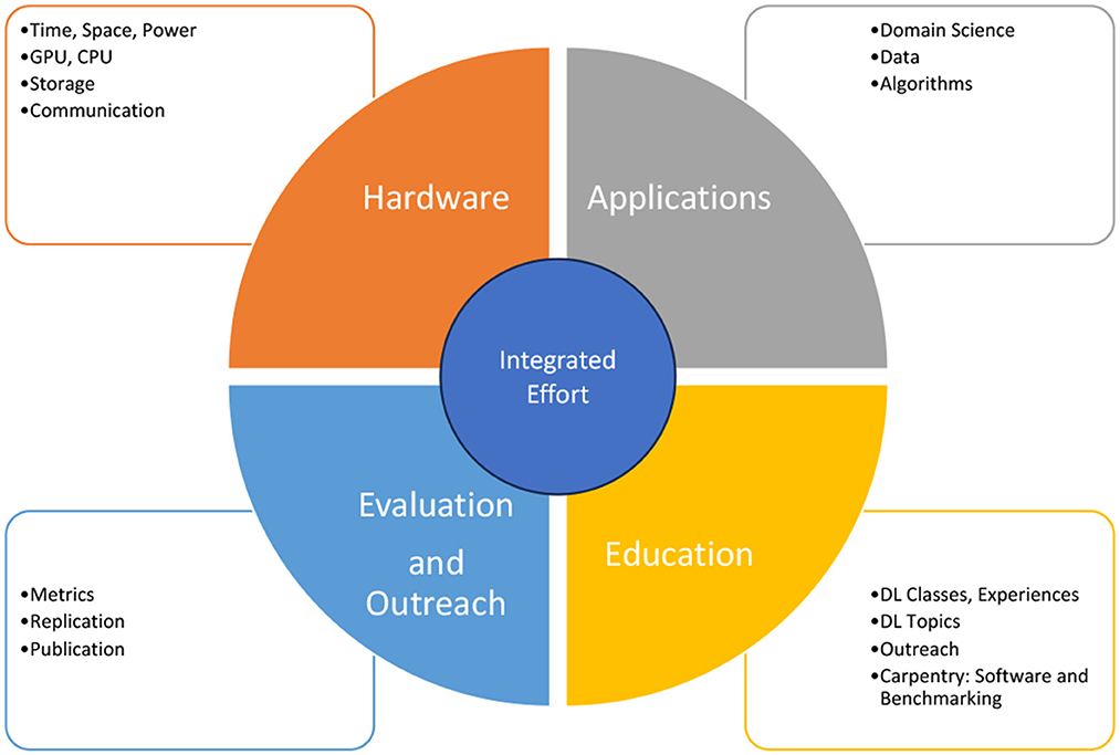
Figure 1. Overview of aspects of opportunities for an integrated educational effort for MLCommons while using applications from the Science Working Group. GPU, graphics processing unit; CPU, central processing unit; DL, deep learning.

Hence, we not only try to identify pathways and exemplars of how such efforts can enhance educational efforts by leveraging expertise from MLCommons into educational efforts, but also consider the unique opportunities and limitations that apply when considering their use within educational efforts.

In general, we look at opportunities and challenges about

• insights from MLCommons toward education and

• insights from education toward MLCommons.

The article is structured as follows: First, we provide an introduction to MLCommons (Section 1.1). Next, we provide some insights about ML in educational settings and the generalization of ML to other efforts (Section 2.1). We then specifically analyze which insights we gained from practically using MLCommons in educational efforts (Section 2.2). After this, we focus on the earthquake forecasting application, describe it (Section 3), and specifically identify our insights in the data management for this application (Section 3). As the application used is time-consuming and is impacted by policy limitations of the educational HPC data system, a special workflow framework has been designed to coordinate the many tasks needed to conduct a comprehensive analysis (Section 3). This includes the creation of an enhanced templated batch queue mechanism that bypasses the policy limitations but makes the management of the many jobs simple through convenient parameter management (Section 3). In addition, we developed a graphical compute coordinator that enables us to visualize the execution of the jobs in a generalized simple workflow system (Section 3). To showcase the performance (Section 4.2) of the earthquake forecasting application, we present data for the runtime (Section 4.2.2) and for the energy (Section 4.2.6). We complete the article with a brief discussion of our results (Section 5).

1.1. MLCommons

MLCommons is a non-profit organization with the goal to accelerate ML innovation to benefit everyone with the help of over 70 members from industry, academia, and government (MLCommons, 2023). Its main focus is developing standardized benchmarks for measuring performance systems using ML while applying them to various applications.

This includes, but is not limited to, application areas from healthcare, automotive, image analysis, and natural language processing (NLP). MLCommons is concerned with benchmarking training (Mattson et al., 2019) and validation algorithms to measure progress over time. Through this goal, MLCommons investigates ML efforts in the areas of benchmarking, data sets in support of benchmarking, and best practices that leverage ML.

MLCommons is organized into several working groups that address topics such as benchmarking related to training, training on HPC resources, and inference conducted on data centers, edge devices, mobile devices, and embedded systems. Best practices are explored in the areas of infrastructure and power. In addition, MLCommons also operates working groups in the areas of Algorithms, DataPerf Dynabench, Medical, Science, and Storage.

The Science Working Group is concerned with improving the science beyond just a static benchmark (Thiyagalingam et al., 2022). The work reported here has been conducted as part of the MLCommons Science Working Group goals.

A list of selected benchmarks for the working groups focusing on inference, training, and science are shown in Table 1.

TABLE 1

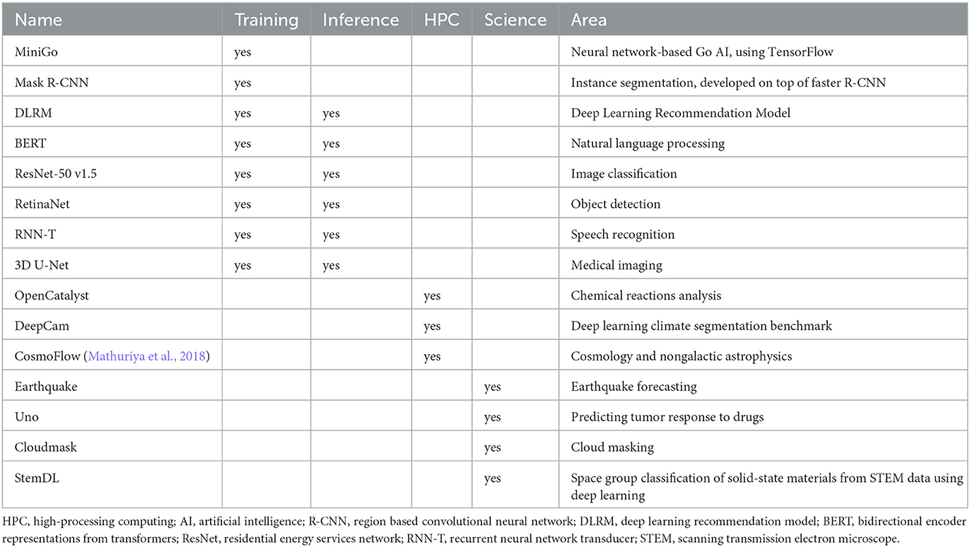
Table 1. MLCommons benchmarks.

Due to the strong affiliation with industry as well as the integration of national labs and academic HPC centers, MLCommons provides a well-positioned starting point for academic participation. Over the years, we have participated significantly in MLCommons's efforts and integrated aspects of MLCommons into our educational activities. Hence, since its inception, we leveraged the MLCommons activities and obtained a number of important educational insights that we discuss in this article.

Summary section 1.1:

• Challenges: The rigor of applying benchmarks requires special attention to reproducible experiments. Educational resources may be limited and a benchmark of a full HPC system may not be possible within an educational computing center while not interrupting other shared usage.

• Opportunities: MLCommons provides a rich set of benchmarks in a variety of areas that comprehensively encompass many aspects of DL applications that are of interest for educational efforts.

2. Insights for educational activities

Next, we discuss our insights while focusing on educational activities. This includes general observations about machine learning methods, libraries, tools and software carpentry, benchmark carpentry, and infrastructure. We then discuss in specific terms how MLCommons-related topics shape our insights. This includes insights of MLCommons while using it in educational settings leading to the potential to create a course curriculum. We then focus on the earthquake application while presenting lessons learned while improving such a large application as part of the code development, data management, and workflow to conduct extensive hyperparameter-based experiments. This leads us to develop tools that simplify monitoring (time and energy), as well as tools to manage jobs and computations while taking into account policy limitations at the HPC center.

2.1. Insights of ML in education

Before starting with the insights from MLCommons on our efforts, we will first consider some of our experience regarding topics taught in educational activities for ML in general. We distinguish ML methods, applications that use or can use ML, the libraries used to apply these methods for applications, software development tools, and finally the infrastructure that is needed to execute them. Understanding these aspects will allow other ML endeavors to benefit from the time-saving, latest technology solutions we have identified that will devote more time to applying ML to real-world problems.

The aim is not to inundate students with all possible facets of machine learning but rather to guide students toward the completion of an interesting, memorable, applicable, real-world project that the student can take and apply to other projects. This necessitates finding a balance between automating the developer setup (providing a ready-to-go environment) and leaving such setup to the student, which can impart knowledge through self-learning. MLCommons provides an ideal starting point for a learning experience as it introduces the student to benchmarking, which is used within the earthquake application discussed later.

2.1.1. ML methods

We list some topics associated with traditional methods in machine learning (ML) and artificial intelligence (AI) that are frequently taught in classes. This includes clustering (exemplified via k-means), image classification, sentiment analysis, time-series prediction, surrogates (a new topic often not taught), and neural networks (with various standard architectures such as convolutional neural networks [CNNs], recurrent neural networks [RNNs], and artificial neural networks [ANNs]). More traditional methods also include modeling techniques such as random forests, decision trees, K-nearest neighbor, support vector machines, and genetic algorithms. These methods are frequently collected into three distinct algorithmic groups: supervised learning, unsupervised learning, and reinforcement learning.

From this small list, we can already see that a comprehensive course curriculum needs to be carefully developed, as it is arduous to cover the topics required in a one-semester course with sufficient depth, but it needs to span the duration of a student's curriculum in AI.

2.1.2. Libraries

There are several diverse libraries and tools that exist to support the development of AI and ML products. As an example, we list a subset of frequently used software libraries and tools that enable the ML engineer and student to write their applications.

First, we note that at the university level, the predominant programming language used for machine learning and data science is Python. This is evident from the success and popularity of sophisticated libraries such as scikit-learn, PyTorch, and TensorFlow. In recent years, we have seen a trend that PyTorch has become more popular at the university level than TensorFlow. Although the learning curve of these tools is significant, they provide invaluable opportunities while applying them to several different applications. As a result, we integrate these tools into our benchmarks and multi-use toolkit, cloudmesh.

In contrast, other specialized classes that focus on the development of faster, graphics processing unit (GPU)-based methods typically use C++ code leveraging the vendor's specialized libraries to interface with the GPUs such as Nvidia CUDA.

2.1.3. Tools and software carpentry

Unfortunately, today's students are not sufficiently exposed to software carpentry at the beginning of their studies, as we found while working with four different student groups from three different universities, despite the university curriculum consisting of Python and AI classes.

To efficiently use the libraries and methods, as well as the infrastructure used to execute software on shared HPC computers, students need a basic understanding of software engineering tools such as a text editor and code management system. A subset of this is often referred to as software carpentry (Wilson et al., 2014). Topics of immediate importance include the ability to (1) obtain a moderate grasp of terminal use with Unix commands, (2) leverage the features of a professional integrated development environment (IDE), (3) be familiar with a code management system and version control, (4) ensure the availability of the code using open sources, (5) understand how to collaborate with others, and (6) utilize queuing systems as used within shared resources managed in HPC centers.

It is vital to instill these industry-standard practices within apprentices new to AI utilization of HPC systems, beyond just the simplest example, to efficiently use the resources and plan benchmark experiments. These skills are key to evolving a beginner's research and class experience toward intermediate and advanced knowledge usable in the industry so they can further contribute to altruist AI applications and the dissemination of work within academia. Moreover, these students will bring valuable and lucrative skill sets with them to their future professional careers.

Although many centers offer Jupyter as an interactive use of the HPC resources, such notebooks are often designed to be simple one-off experiments, not allowing for encapsulation or expansion into other code. Furthermore, the queuing system time imitations within HPC environments hinder the reproducibility of experiments as the time requirements may only allow one experiment as we have experienced with our application.

Pertaining to educational insights, we observed that most students own Microsoft Windows-based desktops and have never come in contact with a terminal using commandline tools. This is backed up by the fact that Microsoft's Windows 10 possesses 68.75% of the operating system (OS) market as of 2023 (Norem, 2023). Hence, the students cannot often navigate a Unix HPC environment, where ML is commonly conducted in a shared resource. This also exacerbates students' manual code expenditure, as Unix commands such as grep, find, and make are typically not known, and automation of the programs building the workflow to execute a benchmark experiment efficiently is limited.

However, as part of our efforts, we found an easy way to not only teach students these concepts but also access HPC machines via a terminal straight from the laptop or desktop. While built-in terminals and shells can be used on macOS and Linux, the ones on Windows are not Unix-like. Nevertheless, the use of the open-source, downloadable Git Bash on Windows systems provides a Unix-like environment. We also leverage Chocolatey, a package manager that mimics the Unix package tools. Alternatively, Windows Subsystem for Linux achieves the same result while directly being able to run Linux in a virtual machine on the computers. However, for students with older or resource-limited machines, the latter may not be an option. To efficiently use the terminal, the elementary use of commands needs to be taught, including the use of a simple command line editor. While leveraging bash on the command line, it becomes easy to develop tutorials and scripts that allow the formulation of simple shell scripts to access the HPC queuing system.

Furthermore, sophisticated programming tools that readily exist in cross-OS portable fashion on the laptop/desktop can be used to develop or improve the code quality of the software. This includes the availability of IDEs (such as PyCharm and VSCode) with advanced features such as syntax highlighting, code inspection, and refactoring. As part of this, applying uniform formatting such as promoted by PEP 8 (www, 2023) increases code readability and uniformity, thereby effortlessly improving collaboration on code by various team members.

Although such IDEs can become quite complex with the evolution of their corresponding toolchains (Fincher and Robins, 2019), in our case, we can restrict their use toward code development and management. As such, habits are immediately introduced that improve the code quality. Furthermore, these tools allow collaborative code development through group editing and group version control management. Together, they help students write correct code that meets industry standards and practices (Tan et al., 2023).

From our experience, this knowledge saves significant effort in time-intensive programs such as Research Experiences for Undergraduates, which typically only last one semester and require the completion of a student project. As part of this, we observed that integrated software carpeting while also integrating IDEs benefits novice students as they are more likely to contribute to existing research activities related to scientific ML applications. Such sophisticated IDEs are offered as free community editions or are available in their professional version for free to students and open-source projects. Such IDEs also provide the ability to easily write markdown text and render the output while writing. This is very useful for writing documentation. Documentation is a necessity in ML research experiences as a lack thereof creates a barrier to entry (Königstorfer and Thalmann, 2022).

As previously mentioned, most recently, these tools also allow writing code remotely, as well as in online group sessions fostering collaboration. Hence, peer programming has become a reality, even if the students work remotely with each other. This is further proven by free online IDEs such as Replit, where students can edit the same file simultaneously (Kovtaniuk, 2022). However, such features have now become an integral part of modern IDEs such as PyCharm and vscode, so the use of external tools is unnecessary. Due to this, we noticed an uptake among students in using the remote editing capabilities of more advanced editors such as PyCharm and vscode; alongside their superiority while developing code, a command editor on the HPC terminal was often avoided. However, this comes with an increased load on the login nodes, which is outweighed by the developers' convenience and code quality while using such advanced editors. HPC centers are advised to increase their capabilities significantly to support such tools while increasing their resources for using them by their customers.

Finally, the common choice for collaborative code management is Git, with successful social coding platforms such as GitHub and GitLab. These code management systems are key for teams to share their developed code and enable collaborative code management. However, they require a significant learning curve. An important aspect is that the code management systems are typically hosted in the open, and the code is available for improvement at any time. We found that students who adopt the open-source philosophy perform considerably better than those who may store their code in a private repository. The openness fosters two aspects:

• First, the code quality improves as the students put more effort into the work due to its openness to the community. This allows students to share their code, improve other code, and gain networking opportunities. Also, perhaps most importantly, this allows scientists to replicate their experiments to ensure similar results and validity.

• Second, collaboration can include research experts from the original authors and researchers that would otherwise not be available at the university. Hence, the overall quality of the research experience for the student increases as the overall potential for success is implicitly accessible to the student.

An additional tool is JupyterLab, created by Project Jupyter. It provides a web browser interface for interactive Python notebooks (with file extension ipynb). The strength here is a rich external ecosystem that allows us to interactively run programs while integrating analysis components to utilize data frames and visualization to conduct data exploration. For example, this is possible by using web browser interfaces to either the HPC-hosted Jupyter notebook editor or Google Colab. The unfortunate disadvantage of using notebooks is that, while the segmentation of code into cells can provide debugging convenience, this format may break proper software engineering practices such as defining and using functions, classes, and self-defined Python libraries that lead to more sustainable and easier-to-manage code. An upside to Jupyter notebooks is that they possess an integrated markdown engine that can provide sophisticated documentation built in; we have also identified that students without access to capable local machines can leverage Google Colab, which is a free platform for using Jupyter notebooks. Jupyter notebooks accessing HPC queues are currently often made available through web-based access as part of on-demand interfaces to the HPC computing resource (uva, 2023).

Regrettably, live collaborative editing of Jupyter notebooks is not yet supported on some platforms such as Replit and PyCharm. However, vscode does support this feature, even within the browser, eliminating the need to download a client. We expect that such features will eventually become available in other tools.

While topical-focused classes such as ML and DL is obviously in the foreground, we see a lack of introducing students to software carpeting and even the understanding of HPC queuing systems in general. Tools such as Jupyter and Colab that are often used in such classes deprive the students often from the needed underlying understanding of efficiently using shared GPU resources for ML and DL.

Hence, students are often ill prepared for software carpeting needs that arise in more advanced applications of DL utilizing parallel and concurrent DL methodologies. Furthermore, programming language classes are often only applied to teaching Python while only emphasizing the language aspects but not with a sustainable, practical software engineering approach. Because ML is a relatively new venture in the computing field, there is not yet a definitive set of standards meant for beginning students. The lack of emphasizing standards as part of teaching activities such as these relates to a general problem at the university level.

We alleviate difficulties such as these encountered within research experience by leveraging a cross-platform cloud-computing toolkit named cloudmesh. This toolkit, alongside our use of professional IDEs and version control, allows students to focus less on manual code expenditures and operating system debugging, and more on HPC use and ML development on data sets such as from the Modified National Institute of Standards and Technology (MNIST), among others. We acknowledge the importance of saving time as it is a precious commodity in research experiences. The use of cloudmesh reduces the entry barrier surrounding the creation of machine learning benchmark workflow applications, as well as our standardized benchmarking system, MLCommons. This system is easily implemented as long as programmers can utilize the capabilities of an industry-standard IDE. Since we emphasize reproducibility and openness with other contributors, then an open-source solution like MLCommons is necessary.

2.1.4. Benchmark carpentry

Benchmark carpentry is not yet a well-known concept while focusing on applying software carpentry, common benchmark software, and experiment management aspects to create reproducible results in research computing. To work toward a consolidated effort of benchmark carpentry, the experiences and insights documented in this article have recently been reported to the MLCommons Science Working Group. Throughout the discussion, we identified the need to develop an effort focusing on benchmark carpentry that goes beyond the aspects typically taught in software carpentry while focusing on aspects of benchmarks that are not covered. This includes a review of other benchmark efforts such as TOP500 and Green500, the technical discussion around system benchmarks including SPEC benchmarks, as well as tools and practices to better benchmark a system. Special effort needs not only to be placed on benchmarking the central processing unit (CPU) and GPU capabilities but also on what effect the impact of the file system or the memory hierarchy has. This benchmarking ensures reproducibility while leveraging the findability, accessibility, interoperability, and reusability principle. Furthermore, using software that establishes not only immutable baseline environments such as Singularity and Docker but also the creation of reproducible benchmark pipelines and workflows using cloudmesh-ee and cloudmesh-cc, is beneficial. Such efforts can also be included in university courses, and the results of developing material for and by the participants can significantly pervade the concept of a standardized benchmarking system such as MLCommons's MLPerf.

2.1.5. Infrastructure

An additional aspect ML students must have exposure to is the need for access to computational resources due to distinct hardware requirements resulting from using an advanced ML framework. One common way of dealing with this is to use preestablished ML environments like Google Colab, which is easy to access and use with limited capability for free (with the option of obtaining a larger computational capability with a paid subscription). However, as Colab is based on Jupyter notebooks, we experience the same disadvantages discussed in Section 2.1.3. Furthermore, benchmarking can become quite expensive using Google Colab depending on the benchmark infrastructure needs.

Another path to obtain resources for machine learning can be found in the cloud. This may include infrastructure-as-a-service and platform-as-a-service cloud service offerings from Amazon, Azure, Google Cloud, Salesforce, and others. In addition to the computational needs for executing neural networks and DL algorithms, we also find services that can be accessed mainly through REpresentational State Transfer Application Programming Interface (REST APIs) offering methods to integrate the technology into the application research easily. Most popular tools focus on NLP, such as translation and, more recently, on text analysis and responses through OpenAI's ChatGPT and Google's Bard.

However, many academic institutions have access to campus-level and national-level computing resources in their HPC centers. In the United States, this includes resources from the Department of Energy and the National Science Foundation (NSF). Such computing resources are accessed mostly through traditional batch scheduling solutions (such as Slurm SLURM, 2003), which allows for sharing limited resources with a large user community. For this reason, centers often implement a scheduling policy that puts significant restrictions on the computational resources that can be used simultaneously and for a limited period. The number of files and the access to a local disk on compute nodes constituting the HPC resources may also be limited. This provides a potential very high entry barrier as these policy restrictions may not be integrated into the application design from the start. Moreover, in some cases, these restrictions may provide a significant performance penalty when data are placed in a slow network file system (NFS) instead of directly in memory (often the data do not fit in memory) or in NVMe storage if it exists and is not restricted on the compute nodes. It is also important to understand that such nodes may also be shared with other users and it is important to provide the infrastructure requirements upfront regarding computation time, memory footprint, and file storage requirements accurately so that scheduling can be performed most expediently. Furthermore, the computing staff maintains the software on these systems and is typically tailored for the HPC environment. It is best to develop with the version provided, which may target outdated software versions. Container technologies reduce the impact of this issue by enabling users of the HPC center to provide their own custom software dependencies as an image.

One of the popular container frameworks for HPC centers is Singularity, and some centers offer Docker as an alternative. As images must bring all the software needed to run a task, they quickly become large in size, and it is not feasible to just copy the image from your local computer but to work with the center to create the image within the HPC infrastructure. This is especially true when a university requires all resources to be accessed through a virtual private network (VPN). Here, one can often see a factor of 10 or more slowdown in transfer and access speeds (Tovar et al., 2021).

All these elements must be learned; establishing an understanding of these subjects can take considerable time. Hence, using HPC resources has to be introduced with specialized educational efforts often provided by the HPC center. However, sometimes these general courses are not targeted specifically to running a particular version of PyTorch or TensorFlow with cuDNN, but just the general aspect of accessing the queues. Although these efforts often fall under the offerings of software carpentry, the teaching objective may fall short as the focus is placed on a limited number of software, supported by the center instead of teaching how to install and use the latest version of TensorFlow. Furthermore, the offered software may be limited in case the underlying GPU card drivers are outdated. Software benchmarks need not only the newest software libraries but also the newest device drivers, which can only be installed by the HPC support team.

Furthermore, specifically customized queues demanding allocations, partitions, and resource requirements may not be documented or communicated to its users, and a burden is placed on the faculty member to integrate this accurately into the course curriculum.

Access to national-scale infrastructure is often restricted to research projects that require following a detailed application process. The faculty supervisor conducts this process and not the student. Background checks and review of the project may delay the application. Additional security requirements, such as the use of Duo Mobile, SSH keys, and other multifactor authentication tools must be carefully taught.

In case the benchmark includes environmental monitoring such as temperatures on the CPU/GPU and power consumption, access may be enabled through default libraries and can be generalized while monitoring the environmental controls over time. However, HPC centers may not allow access to the overall power consumption of entire compute racks as it is often very tightly controlled and only accessible to the HPC operational support staff.

2.2. Insights of MLCommons in education

The MLCommons benchmarks provide a valuable starting point for educational material addressing various aspects of the machine and deep learning ecosystem. This includes benchmarks targeted to a variety of system resources from tiny devices to the largest research HPC and data systems in the world while being able to adapt and test them on platforms between these two extremes. Thus, they can become ideal targets for adaptation in AI classes that want to go beyond typical introductory applications such as MNIST that run in a small amount of time.

We have gained practical experience while adapting benchmarks from the MLCommons Science Working Group while collaborating with various universities and student groups from the University of Virginia (UVA), New York University, and Indiana University. Furthermore, it was used at Florida A&M University as a research experience for undergraduates (REU) and is now executed at the UVA as research activity by a past student from the REU (Fleischer et al., 2022). The examples provide value for classes, capstones, REUs, team project-oriented software engineering and computer science classes, and internships.

We observed that traditional classes limit their resource needs and the target application to a very short period so assignments can be conducted instantly. Some MLCommons benchmarks go well beyond this while confronting the students not only with the theoretical background of the ML algorithm but also with big data systems management, which is required to execute benchmarks due to their data and time requirements. This is especially the case when hyperparameters are to be identified to derive scientifically accurate examples. It is also beneficial in that it allows the students to explore different algorithms applied to these problems.

From our experiences with these various efforts, we found that the following lessons provided significant add-on learning experiences:

• Teamwork. Students benefit from focusing on the success and collaboration of the entire team rather than mere individualism, as after graduation, students may work in large teams. This includes not only the opportunity for pair programming but also the fact that careful time planning in the team is needed to succeed. This also includes how to collaborate with peers using professional, industry-standard coding software and management of code in a team through a version control system such as Git. As others point out (Raibulet and Fontana, 2018), we also see an increase in enthusiasm and appreciation of teamwork-oriented platforms when such aspects are employed in coding courses. While courses may still focus on the individual's progress, an MLCommons Benchmark benefits from focusing on grading the team and taking the entire project and team progress into a holistic grade evaluation.

• Interdisciplinary research. Many of the applications in MLCommons require interdisciplinary research between the domain scientists, ML experts, and information technology engineers. As part of the teamwork, students have the opportunity to participate not only within their discipline but learn about how to operate in an interdisciplinary team. Such multidisciplinary experience not only broadens their knowledge base but also strengthens their market viability, making them attractive candidates for diverse job possibilities and career opportunities in the ever-evolving technological landscape (Zeidmane and Cernajeva, 2011).

• System benchmarking versus science benchmarking. Students can learn about two different benchmarking efforts. The first is system-level benchmarking in which a system is compared based on a predefined algorithm and its parameters measuring system performance. The second is the benchmarking of a scientific algorithm in which the quality of the algorithms is compared with each other, where system performance parameters are a secondary aspect.

• Software ecosystem. Students are often using a course-provided, limited, custom-defined environment prepared explicitly for a course that makes course management for the teacher easier but does not expose the students to various ways of setting up and utilizing the large variety of software related to big data systems. This includes setting up Python beyond the use of Conda and Colab notebooks, the use of queuing systems, containers, and cloud computing software for AI, DL, and HPC experiments as well as other advanced aspects of software engineering. Benchmarking introduces these concepts to students in a variety of configurations and environments, providing them with a more research- and industry-like approach to managing software systems.

• Execution ecosystem. While in-class problems typically do not require as many computing resources, some of the examples in MLCommons require a significant organizational aspect to select and run meaningful calculations that enhance the accuracy of the results. Careful planning with workflows and the potential use of hybrid heterogeneous systems significantly improves the awareness to deal with not only the laptop but also the large available resources students may get access to while leveraging flagship-class computing resources, or their own local HPC system when available. Learning to navigate an HPC system is imperative to teach to students and can be augmented by professor-created toolkits and platforms (Zou et al., 2017). We found it necessary to provide additional documentation to address the staff-provided HPC manual while focusing on specific aspects that are not general in nature but are related to group and queue management specifically set up for us by staff. This includes documentation about the accounting for system policies, remote system access, and frugal planning of experiments through the prediction of runtimes and the planning of hyperparameter searches (Claesen and De Moor, 2015; von Laszewski et al., 2022). This can also include dealing with energy consumption and other environmental parameters.

• Parallelization. The examples provide a basis for learning about various parallelization aspects. This includes the parallelization on not only the job level and hyperparameters searches but also on the use of parallelization methods provided by large-scale GPU-based big data systems.

• Input/Output (IO) data management. One other important lesson is the efficient and effective use of data stores to execute. For example, DL algorithms require a large number of fast IO interactions. Having access to sufficient space to store potentially larger data sets is beneficial. Also, the time needed to send data from the external storage to the GPU should be small to ensure that the GPUs have sufficient data to perform well without bottleneck. Such management is vital to be taught within education as the entirety of ML depends on the organization of data (Shapiro et al., 2018).

• Data analysis. The examples provide valuable input to further enhance abilities to conduct non-trivial data analysis through advanced Python scripts while integrating them in coordinated runs to analyze log files that are created to validate the numerical stability of the benchmarks. This includes the utilization of popular data analysis libraries (such as Pandas) as well as visualization frameworks (such as Seaborn). It also allows students to focus on identifying a result that can be communicated in a professional manner.

• Professional and academic communication. The results achieved need to be communicated to a larger audience and the students can engage in a report, paper, and presentation writing opportunities addressing scientific and professional communities.

• Benefits to society. The MLCommons benchmarks are including opportunities to improve the quality of ML algorithms that can be applied to societal tasks. Obviously, improving benchmarks such as earthquake forecasting are beneficial to society and can motivate students to participate in such educational opportunities.

2.2.1. MLCommons DL-based proposed course curriculum

In this section, we explore the idea to potentially create a course curriculum utilizing the MLCommons effort. For this to work and focus for MLCommons, the course can focus on DL while using examples from MLCommons benchmarks as well as additional enhancements into other topics that may not be covered.

In contrast to other courses that may only focus on DL techniques, this course will have the requirement to utilize significant computational resources that are, for example, available on many campuses as part of an HPC or a national scale facility such as NSF's Access. Alternatively, Google Colab can be used; however, it will have the disadvantage of not using HPC resources from local or national HPC centers as discussed earlier.

1. Course overview and introduction: Here the overview of the course is provided. Goals and expectations are explained and an introduction to deep learning is provided. This includes the history and applications of DL, a basic introduction to optimization technologies and neural networks, and the connection between MLCommons Applications is presented.

2. Infrastructure and benchmarking: An overview of MLCommons-based DL applications and benchmarks are discussed and will include a wide variety reaching from tiny devices to supercomputers and hyperscale clouds. Google Colab will be introduced. Practical topics such as using ssh and batch queues are discussed. An explicit effort is placed on using a code editor such as PyCharm or VSCode. Elementary software infrastructure is discussed while reviewing Python concepts for functions, classes, and code packaging with pip. The use of GitHub is introduced.

3. CNNs: A deeper understanding is taught by focusing on CNNs. The example of Mask R-CNN is explained.

4. RNNs: RNNs are taught and applications of RNNs are discussed. The RNN-T application focusing on speech recognition is presented and analyzed.

5. NLP: As NLP has such a big impact on industry and academia, additional lectures in that area are presented. This includes large language models, analyzing text, applications of NLP, language translation, and sentiment analysis. Practical examples are introduced while looking at ChatGPT. From MLCommons, the applications DLRM, BERT, and RNN-T are discussed.

6. Project presentations: The last part of the class is focused on a project presentation that students can conduct in a team or individually. It should showcase an application and performance results on one or multiple HPC data systems, or include an improvement to an existing MLCommons benchmark. It is expected that the students write a high-quality project report. Ideally, each team will submit its result to MLCommons. A good start here is the Science Working Group as it provides rolling submissions and its focus is accuracy and not speed, which is often a topic of interest in academia.

7. Submitting expanding MLCommons benchmarks: The results obtained can be also submitted to MLCommons. Here we see two opportunities: first the submission of results from standardized benchmarks provided by MLCommons and, second, the inclusion of new scentific application results submitted to the MLCommons Science Working group.

Adaptations of this material are possible and can be made accordingly to stay up to date with community AI developments as well as efforts newly covered in MLCommons. The semester-long project is accompanied by biweekly practical mini-assignments showcasing selected results and implementations of a particular topic. The final outcome will be a project report. Grading and integration can be done based on the instructors and the university course requirements that university policies may govern. Practically, we believe that grading the project will be sufficient; however, we observed that weekly graded assignments may be needed to compete with other weekly homework-oriented graded classes that require immediate attention by the students. The curriculum can be divided into several sections that can be taught over a semester in either a graduate or undergraduate class or a combination thereof. The curriculum could be used in its entirety, or selected aspects could be taught.

Summary section 2:

• Challenges: Students lack knowledge of software carpentry despite taking programming and AI classes at universities. Software carpeting tools such as terminals, command line tools, and IDEs are not sufficiently utilized although they provide significant benefits for professional code development and management of shared resources. Today's DL students often have only knowledge about Jupyter notebooks or Google Collab resulting in one-cell-at-a-time-oriented programming rather than a proper more sophisticated software engineering approach. Using computing resources at HPC centers may pose a considerable on-ramp hurdle, especially when combined with queuing systems and container technologies that vary in their implementation between centers; specialized documentation must be available.

• Opportunities: Software carpeting could be offered as an additional class and made a prerequisite for taking AI classes, or become an integral part of the DL experience. This should include learning about terminal commands, accessing queuing systems, IDEs, code management, and collaborative code development going beyond the usage of Jupyter notebooks. Benchmark carpentry should be offered in addition to software carpentry while focusing on unique aspects of reviewing common benchmark practices and applying them to DL applications. Tools such as cloudmesh used in several MLCommons applications allow leveraging creating simple standardized interfaces to time-based benchmarks and the display of the results in a human-readable form. Exposing students to knowledge about shared HPC resources used for DL rather than just reusing cloud resources offers a deeper understanding of resource-efficient resource utilization in a resource-starved environment as well as the costs associated with them having an impact on affordable benchmarks. MLCommons covers a wide variety of topics and it is conceivable to develop a comprehensive course curriculum around it that could be either used in its entirety or adapted based on interests as well as selectively taught. To address variations in the HPC technologies used, center documentation can be developed by an organization but may have to be adapted to simplify it while focusing on storage, compute, and container technologies and specifics offered. This course curriculum provides the opportunity to emphasize teamwork while focusing on a larger project.

3. Earthquake forecasting

While we so far have focused on the general applicability of MLCommons benchmarks as potential options to develop an educational curriculum, we focus next on an exemplar for a potential semester-long project and their insights toward the goal of using it as an educational tool.

Although MLCommons has many applications, we decided to use an application from the MLCommons Science Working Group as we most closely work as part of this group. It has four major benchmarks as documented in Thiyagalingam et al. (2022) in von Laszewski et al. (2023).

However, here we focus on the earthquake benchmark code that creates a Time Series Evolution Operator (TEvolOp) to be applied to several scientific applications such as hydrology and COVID-19 predictions. We focus on this application because, in contrast to other MLCommons applications it is written as a Jupyter notebook and therefore intercepts with many educational efforts using Jupyter notebooks. We restrict our report to the efforts related to earthquake forecasting as it is one of the first applications from the MLCommons Science Working Group that have been used in educational class projects.

The scientific objective of the earthquake benchmark is to extract the evolution using earthquake forecasting while utilizing time series forecasting.

The earthquake benchmark uses a subset of the overall earthquake data set for the region of Southern California. While conventional forecasting methods rely on statistical techniques, we use ML for extracting the evolution and testing the effectiveness of the forecast. As a metric, we use the Nash-Sutcliffe Efficiency (NSE) (Nash and Sutcliffe, 1970). Other qualitative predictions are discussed in Fox et al. (2022).

One of the common tasks when dealing with time series is the ability to predict or forecast them in advance. Time series capture the variation of values against time and can have multiple dimensions. For example, with earthquake forecasting, we use geospatial data sets that have two dimensions based both on time and spatial position. The prediction is considerably easier when we can identify an evolution structure across dimensions. For example, by analyzing earthquake data, we find a strong correlation between nearby spatial points. Thus, nearby spacial points influence each other and simplify the time-series prediction for an area. However, as earthquake faults and other geometric features are not uniformly distributed, such correlations are often not clearly defined in spatial regions. Thus it is important to look not only at the region but also at the evolution in time series. This benchmark extracts the evolution of time series applied to earthquake forecasting.

3.1. Earthquake data

The data for this earthquake are described in Thiyagalingam et al. (2022). It uses a subset of the earthquake data from the United States Geological Survey (USGS) focused on Southern California between latitude 32°N to 36°N and longitude: −120°S to −114°S). The data for this region cover all earthquakes since 1950. The data include four measurements per record: magnitude, spatial location, depth from the crust, and time. We curated the data set and reorganized it in different temporal and spatial bins. “Although the actual time lapse between measurements is one day, we accumulate this into fortnightly data. The region is then divided into a grid of 40 × 60 with each pixel covering an actual zone of 0.1 deg × 0.1 or 11km × 11km grid. The dataset also includes an assignment of pixels to known faults and a list of the largest earthquakes in that region from 1950. We have chosen various samplings of the dataset to provide both input and predicted values. These include time ranges from a fortnight up to four years. Furthermore, we calculate summed magnitudes and depths and counts of significant quakes (magnitude < 3.29)” (Fox et al., 2022). Table 2 depicts the key features of the benchmark (Thiyagalingam et al., 2022).

TABLE 2

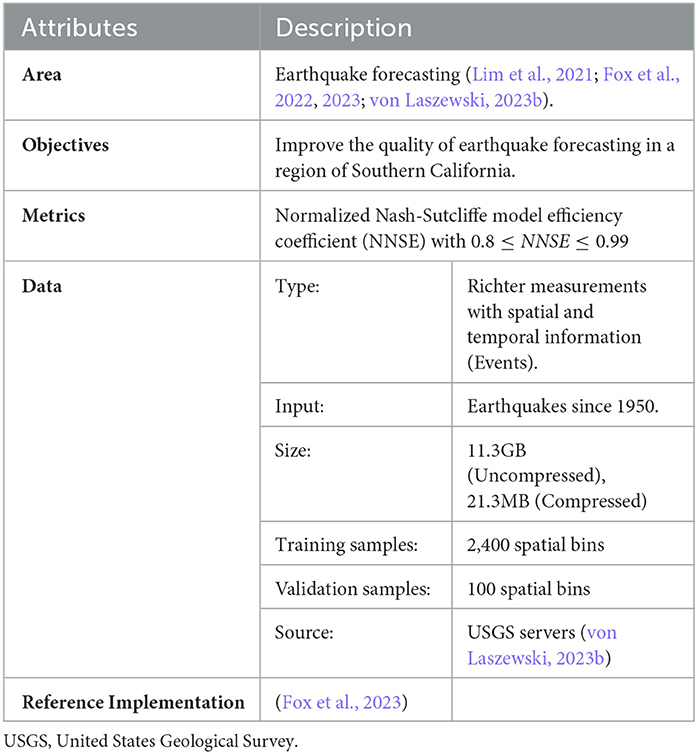
Table 2. Summary of the earthquake TEvolOp benchmark.

3.1.1. Implementation

The reference implementation of the benchmark includes three distinct deep learning-based reference implementations. These are a long short-term memory (LSTM)–based model, a Google Temporal Fusion Transformer (TFT) (Lim et al., 2021)–based model, and a custom hybrid transformer model. The TFT-based model uses two distinct LSTMs, covering an encoder and a decoder with a temporal attention-based transformer. The custom model includes a space-time transformer for the decoder and a two-layer LSTM for the encoder. Figure 2 shows the TFT model architecture. Each model predicts NSE and generates visualizations illustrating the TFT for interpretable multi-horizon time-series forecasting (Lim et al., 2021).

FIGURE 2

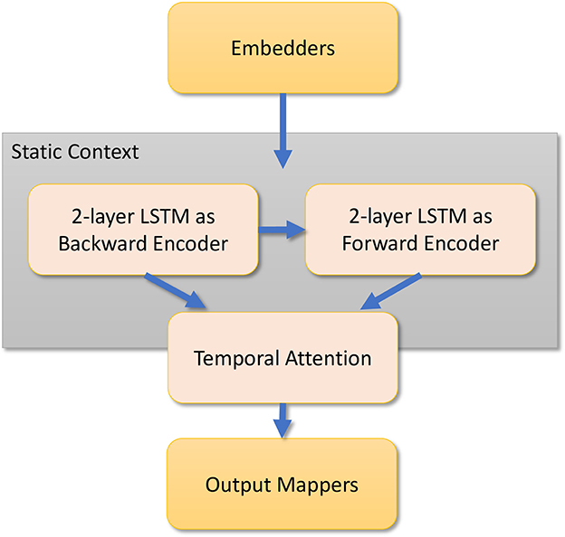
Figure 2. Temporal fusion transformer model architecture (Fox et al., 2022). LSTM, long short-term memory.

For this article, we adopted the same calculations as defined in Fox et al. (2022): “We have chosen various samplings of the dataset to provide both input and predicted values. These include time ranges from a fortnight up to 4 years. Further, we calculate summed [according to Equation (1)] magnitudes and averaged depths (according to Equation (2)) and counts of significant earthquakes [magnitude > 3.29, Equation (3)]. We use the concept of energy averaging when there are multiple events in a single space-time bin. Therefore, the magnitude assigned to each bin is defined in Equation (1) as 'log(Energy)' where we sum over events of individual magnitudes m_event. We also use energy averaging defined in Equation (2) for quantities Q_bin such as the depth of an earthquake that needs to be weighted by their importance when averaging over a bin.”

$\begin{array}{ll}{m}_{bin}=log(Energy)=\frac{1}{1.5}{log}_{10}{\displaystyle \sum _{inbin}^{Events}}10^{1.5m_{event}}& (1)\end{array}$

$\begin{array}{ll}EnergyweightedQuantity{Q}_{bin}=\frac{{\displaystyle \sum _{inbin}^{Events}}10^{1.5m_{event}}{Q}_{event}}{{\displaystyle \sum _{inbin}^{Events}}10^{1.5m_{event}}}& (2)\end{array}$

$\begin{array}{ll}Multiplicit{y}_{bin}={\displaystyle \sum _{inbin}^{Events}}Multiplicit{y}_{event}subjecttoaconstraint& (3)\end{array}$

In this article, we only focus on the TFT implementation. The TFT inputs and outputs are described next (Fox et al., 2022).

• Static Known Inputs (five inputs): four space-filling curve labels of fault grouping, linear label of pixel.

• Targets (four targets): m_bin(F : Δt, t) for Δt = 2, 14, 26, 52 weeks. Calculated for t − 52 to t for encoder and t to t + 52 weeks for decoder in 2 week intervals. 104 predictions per sequence.

• Dynamic known inputs (13 inputs): P_l(cos_Full) for l = 0 to 4 cos_period(t), sin_period(t) for period = 8, 16, 32, 64.

• Dynamic unknown inputs (nine inputs): Energy-averaged depth, multiplicity, multiplicity m > 3.29 events m_bin(B : Δt, t) for Δt = 2, 4, 8, 14, 26, 52 weeks.

These data can be input based on the time series. Backward data can be taken up to 1 year before the current date, and forward data can be taken up to 4 years into the future. The data are then enriched with the LSTM models on time and other factors like spacial location, fault grouping and energy produced at location. Feature selection is done. The data are then fed into an attention learning module, which learns trends and more complex relationships based on the data across all time steps and can apply this knowledge to any number of time steps. More feature selection is done. Then finally the data are run through quantile regression. The loss is calculated by mean aboslute error (MAE). This repeats until all epoch runs are done and the iteration that had the lowest loss is used to create predictions. Normalized Nash Sutcliffe efficiency (NNSE) and mean squared error (MSE) are used as a goodness of fit metric.

More details of the TFT model applied to the earthquake application are presented in Fox et al. (2022). More general details about TFT models can be found in Lim et al. (2021).

3.1.2. Insights into development of the code

The original code was developed with the goal of creating a DL method called TEvolOp to apply special time-series evolution for multiple applications including earthquake, hydrology, and COVID-19 prediction. The code was presented in a large Python Jupyter notebook on Google Colab. Due to the integration of multiple applications (hydrology and COVID-19), the code is complex and challenging to understand and maintain. For this reason, the total number of lines of 13,500 was reduced by more than 2,400 lines when the hydrology and the COVID code were removed. However, at the same time, we restructured the code and reached a final length of about 11,100 lines of code. The code was kept as a Jupyter notebook in order to test the applicability of benchmarking applications presented at notebooks rather than converting it into a pure Python script. The code included all definitions of variables and hyperparameters in the code itself. This means that the original code needed to be changed before running it in case a hyperparameter needed to be modified.

This code has some challenges that future versions ought to address. First, the code includes every aspect that is not covered by TensorFlow and contains a customized version of TFT. Second, due to this the code is very large, and manipulating and editing the code are time-consuming and error-prone. Third, as many code-related parameters are managed still in the code, running the same code with various parameters becomes cumbersome. In fact, multiple copies of the code need to be maintained when new parameters are chosen, instead of making such parameters part of a configuration file. Hence, we started moving toward the simplification of the code by introducing the concept of libraries that can be pip installed, as well as adding gradually more parameters to configuration files that are used by the program.

The advantage of using a notebook is that it can be augmented with lots of graphs that give updates on the progress and its measurement accuracy. It is infeasible for students to use and replicate the run of this notebook on their own computers as the runtime can be up to two days. Naturally, students use their computers for other purposes and need to be able to use them on the go, not having the luxury to dedicate such a prolonged time to running a single application. Hence, it is desirable to use academic HPC centers that provide interactive jobs in the batch queues in which Jupyter notebooks could be run. However, running such a time-consuming interactive job is also not possible in most cases. Instead, we opted to use Jupyter notebooks with a special batch script that internally uses Papermill (Papermill, 2020) and leverages an HPC queuing system to execute the notebook in the background. Papermill will execute the notebook and include all cells that have to be updated during runtime, including graphics in a separate runtime copy. The script we developed needed to be run multiple times with different hyperparameters such as the number of epochs. As the HPC system is a heterogeneous GPU system having access to A100, V100, P100, and RTX2080 graphics cards, the choice of the GPU system must be able to be configurable. Hence, the batch script includes the ability to also read in the configuration file and adapt itself to the needed parameters so such parameters can be separated from the actual notebook. This is controlled by a sophisticated but simple batch job generator, which we discuss in Section 3.

Summary choosing the earthquake benchmark application:

• Opportunities: Using a scientific application as a project within the educational efforts allows students to identify pathways on how to apply DL knowledge to such applications.

Furthermore, we have chosen an application written as a Jupyter notebook to identify if students have an easier time with it and to see if benchmarks can be easily generated if notebooks are used instead of just Python programs. We identify that existing tools such as Papermill can provide the ability to run Jupyter notebooks in queuing systems while running them as tasks in the background and capturing cell output.

• Challenges: Understanding a scientific application can be quite complex. Having a full implementation using DL for it, still provides challenges as data and algorithm dependencies need to be analyzed and domain knowledge needs to be communicated to gain deeper understanding. It is important to separate the runtime environment variables as much as possible from the actual notebook. The coordination of such variables can be challenging and tools such as cloudmesh-ee make such integration simple.

3.2. Insights into data management from the earthquake forecasting application

In data management, we are concerned with various aspects of the data set, the data compression and storage, and the data access speed. We discuss insights into each of them that we obtained while looking at the earthquake forecast application.

3.2.1. Data sets

When dealing with data sets, we typically encounter several issues. These issues are addressed by the MLCommons benchmarks and data management activities so that they provide ideal candidates for education without spending an exorbitant amount of time on data. Such issues typically include access to data without privacy restrictions, data preprocessing that makes the data suitable for DL, and data labeling in case they are part of a well-defined MLCommons benchmark. Other issues include data bias, noisy or missing data, as well as overfitting while using training data. Typically the MLCommons benchmarks will be designed to limit such issues. However, some benchmarks such as the science group benchmarks, which are concerned with improving the science, have the option to potentially address these issues in order to improve the accuracy. This could even include injecting new data and different preprocessing methods.

3.2.2. Data compression

An issue of utmost importance, especially for large data sets, is how the data are represented. For example, we found that the original data set was 11 GB for the earthquake benchmark. However, we found the underlying data were a sparse matrix, and was easily lossless compressed by a factor of 100. This is significant, as in this case the entire data set can be stored in GitHub or moved quickly into memory. The compressed xz archive file is only 21 MB, and downloading only the archive file using wget takes 0.253 s on the HPC. In case the data set and its repository are downloaded with Git, we note that the entire Git repository is 108MB (von Laszewski, 2023b). On the Rivanna Supercomputer, downloading this compressed data set only takes 7.723 s. Thus, it is preferred to just download the data using wget. In both cases, the data are compressed. To uncompress, the data will take an additional 1min 2.522 s. However, if we were to download the data in uncompressed form, it would take ≈ 3 h 51 s. The reduction in time is due to the fact that the data are sparse, and the compression allows a significant reduction needed to store and thus transfer the data.

From this simple example, it is clear that MLCommons benchmarks can provide students insights into how data are managed and delivered to, for example, large-scale computing clusters with many nodes while utilizing compression algorithms. We next discuss insights into infrastructure management while using file systems in HPC resources. While often object stores are discussed to host such large data sets, it is imperative to identify the units of storage in such object stores. In our case, an object store that would host individual data records is not useful due to the vast number of data points. Therefore, the best way to store these data, even in an object store, is as a single entry of compressed overall data. Other MLCommons Science Working Group benchmarks have data sets in the order of 500 GB–12 TB. Other tools, such as Globus transfer, can be used to download larger data sets. Obviously, these sets need special considerations when placed on a computing system where the students' storage capacities may be limited by policy.

3.2.3. Data access

Besides having proper data and being able to download them efficiently from the location of storage, it is imperative to be able to access it in such a way that the GPUs used for DL are being fed with enough data without being idle. Our performance results were somewhat surprising and had a devastating effect on the overall execution time. We found that the performance was more than twice as fast on the personal computer while using an RTX3090 in contrast to using the HPC center recommended file systems when using an A100. For this reason, we have made a simple test and measured the performance to read access the various file systems. The results are shown in Table 3, which include not only various file systems at the UVA's Rivanna HPC but also a comparison with a personal computer.

TABLE 3

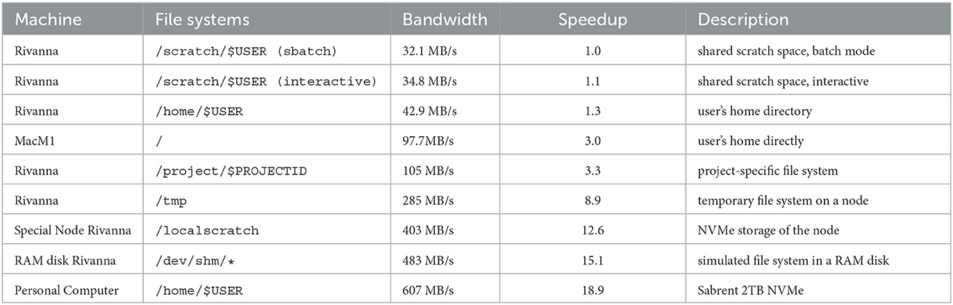
Table 3. File transfer performance of various file systems on Rivanna and personal computers.

Based on this observation, it was of great disadvantage to consider running the earthquake benchmark on the regularly configured HPC nodes as they ran on some resources for almost 24h due to the policy limit the Rivanna system allows for one job. Hence, we were allowed to use a special compute node that has additional non-volatile memory express (NVMe) storage available and accessible to us. On those nodes (in the Table listed as /localscratch), we were able to obtain a very suitable performance for this application while having a 10-fold increase in access in contrast to the scratch file system and almost double the performance given to us on the project file system. The /tmp system—although fast—was not sufficiently large for our application and performs slower than the /localscratch setup for us. In addition, we also made an experiment using a shared memory-based-hosted file system in the nodes random-access memory (RAM).

What we learn from this experience is that an HPC system must provide a fast file system locally available on the nodes to serve the GPUs adequately. The computer should be designed from the start to not only have the fastest possible GPUs for large data processing but also have a very fast file system that can keep up with the data input requirements presented by the GPU. Furthermore, in case updated GPUs are purchased, it is not sufficient to just take the previous-generation motherboard, CPU processor, and memory but to update the hardware components and include a state-of-the-art compute node. This often prevents the repurposing of the node while adding just GPUs due to inefficient hardware components that cannot keep up with the GPU's capabilities.

Summary of data management aspects:

• Challenges: Scientific applications require at times large-scale storage spaces that can be provided while using HPC compute centers. The speed of accessing the data depends on where the data is and can be stored in the HPC system. Performance between systems can vary drastically showcasing differences between shared, non-shared, NVMe-based storage, and in-memory storage volumes.

• Opportunities: Input data needs to be placed on appropriate storage options to satisfy the fastest possible access guided by benchmarks. As scientific data are often sparse, they could be significantly compressed, and the time to access the data to move them and uncompress them is often much shorter than the time one needs to load the uncompressed data. Access to a server to its local storage system is essential and must be provided by the HPC center. Instead of old-fashioned HDDs or even SSDs, the fastest NVMe storage should be provided.

3.3. Insights into DL benchmark workflows

As we are trying to benchmark various aspects of the applications and the systems utilizing DL, we need to be able to easily formulate runtime variables that take into account different control parameters either of the algorithm or the underlying system and hardware.

Furthermore, it is beneficial to be able to coordinate benchmarks on remote machines either on a single system or while using multiple systems in conjunction with hybrid and heterogeneous multi-HPC systems. Thus, if we change parameters for one infrastructure, it should be possible to easily and automatically be applied to another infrastructure to identify the impact on both. These concepts are similar to those found in cloud and grid computing for job services (von Laszewski et al., 2002) and for workflows (von Laszewski, 2005; von Laszewski et al., 2007). However, the focus here is on ensuring the services managing the execution are provided and controlled by the application user and not necessarily by the cloud or HPC provider. Thus, we distinguish the need for a workflow service that can utilize heterogeneous HPC systems while leveraging the same parameter set to conduct a benchmark for comparison by either varying parameters on the same or other systems. Such a framework is presented by von Laszewski et al. (2022, 2023) and is based on our earlier work on workflows in clouds and grids.

In addition, we need a mechanism to create various runs with different parameters. One of the issues we run into is that often our runtime needs exceed that of a single job submission. Although job arrays and custom configurations exist, they often lead to longer runtimes that may not be met by default policies used in educational settings. Thus, it is often more convenient to create jobs that fall within the limits of the HPC center's policies and split the benchmarking tasks across a number of jobs based on the parameter permutations. This also allows easier parallelization.

For this reason, von Laszewski et al. have implemented the cloudmesh Experiment Executor (cloudmesh-ee) that provides an easy-to-use batch job generator, creating parallel jobs based on a permutation of experiment parameters that are defined in a configuration file. The tool creates for each job its own subdirectory, copies the code and configuration files into it, and creates a shell script that lists all jobs to be submitted to the queuing system. This also has the advantage that Jupyter notebooks can easily be integrated into this workflow component, as a local copy is generated in each directory and the output for each cell is created during the program execution.

Furthermore, we need a simple system to measure the performance and energy, while communicating the data in an easy fashion to the users. This system was developed by von Laszewski and contains two components: (a) a general stopwatch and (b) a mechanism to monitor the GPU as discussed in Section 3.

We describe these systems briefly while focusing on their applicability for benchmarks.

3.3.1. Cloudmesh monitoring

For years, we have provided a convenient StopWatch package in Python to conduct time monitoring (von Laszewski, 2022a). It is very easy to use and is focused on runtime execution monitoring of time-consuming portions in a single-threaded Python application. Although MLCommons provides its own time-measuring component, called mllog, it is clear from the name that the focus is to create entries in a log file that is not easily readable by a human and may require postprocessing to make it usable. In contrast, our library contains not only simple labeled start and stop methods, but it also provides a convenient mechanism to print human-readable customizable performance tables. However, it is possible to also generate a result table in other formats such as comma-separated values (CSV), JavaScript object notation (JSON), YAML ain't markup language (YAML), shorthand for text (TXT), and others. Human readability is especially important during a debugging phase when benchmarks are developed. Moreover, we also have developed a plugin interface to mllog that allows us to automatically create mllog entries into an additional log file, so the data may be used within MLCommons through specialized analytics programs. A use case is depicted next (we have omitted other advanced features such as function decorators for the StopWatch to keep the example simple).

 

      from cloudmesh.common.StopWatch

      import StopWatch

      # ...

      StopWatch.event("start")

        # this where the timer starts

      StopWatch.start("earthquake")

        # this is when the main benchmark

        # starts

      # ... run the earthquake code

      # ... additional timers could be

      #     used here

  

      with StopWatchBlock("calc"):

        # this is how to use a block timer

        run_long_calculation()

      StopWatch.stop("earthquake")

      # this is where the main benchmark

      # ends

      StopWatch.benchmark()

      # prints the current results

To also have direct access to MLCommons events, we have recently added the ability to call a StopWatch.event.

In addition to the StopWatch, we have developed a simple command line tool that can be used, for example, in batch scripts to monitor the GPU performance characteristics such as energy, temperature, and other parameters (von Laszewski, 2022b). The tool can be started in a batch script as follows and is currently supporting NVIDIA GPUs:

      cms gpu watch --gpu=0 --delay=0.5 --

          dense > gpu0.log &

Monitoring time and system GPU information can provide significant insights into the application's performance characteristics. It is significant for planning a time-effective schedule for parameters while running a subset of planned experiments.

3.3.2. Analytics service pipelines

In many cases, a big data analysis is split up into multiple subtasks. These subtasks may be reusable in other analytics pipelines. Hence, it is desirable to be able to specify and use them in a coordinated fashion, allowing the reuse of the logic represented by the analysis. Users must have a clear understanding of what the analysis is doing and how it can be invoked and integrated.

The analysis must include an easy-to-understand specification that encourages reuse and provides sufficient details about its functionality, data dependency, and performance. Analytics services may have authentication, authorization, and access controls built-in that enable access by users controlled by the service providers.

The overall architecture is depicted in Figure 3A. It showcases a layered architecture with components dealing with batch job generation, storage management, compute coordination, and monitoring. These components sit on top of other specialized systems that can easily be ported to other systems while using common system abstractions.

FIGURE 3

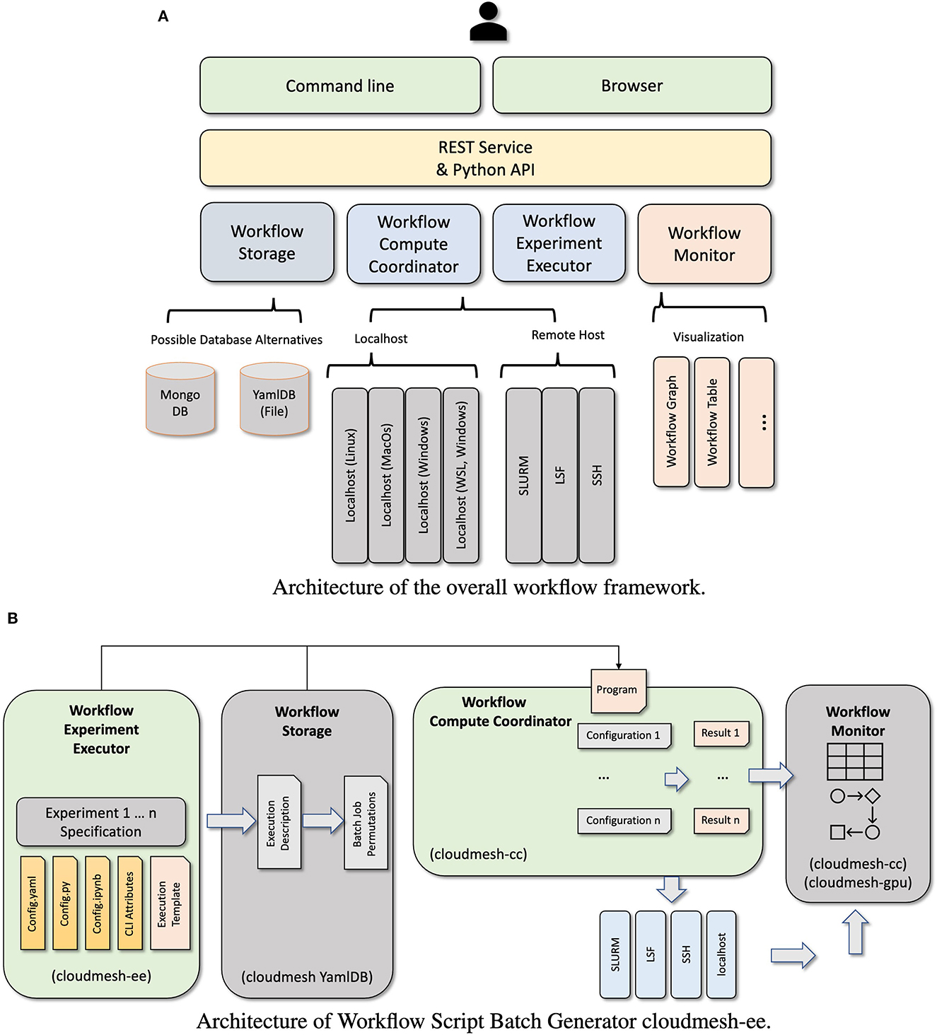
Figure 3. Architecture of the cloudmesh workflow service framework. (A) Architecture of the overall workflow framework. (B) Architecture of Workflow Script Batch Generator cloudmesh-ee. REST, REpresentational State Transfer; API, application programming interface; DB, database; WSL, windows subsystem for linux; SLURM, simple linux utility for resource management; LSF, load sharing facility; SSH, secure shell.

Instead of focusing on the details of this architecture, we found that the high-level use of it is very important as part of the educational activities which also have an implication in general on the use within any research activity.

We identified three beneficial concepts as part of the analytics service pipelines (see Figure 4):

• Selection—Instead of performing all possible benchmarks, a specific parameter set is selected and only that is run.

• Competition—From a number of runs, a result is identified that is better than others. This may be, for example, the best of n benchmark runs.

• Cooperation—A number of analytics components are run (possibly in parallel) and the final result is a combination of the benchmark experiments run in cooperation. This, for example, could be that the job is split across multiple jobs due to resource limitations.

FIGURE 4

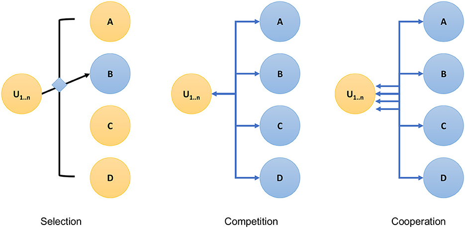
Figure 4. Service interaction.

In the earthquake code, we have observed all three patterns are used in the benchmark process.

3.3.3. Workflow compute coordinator

Within HPC environments, scientific tasks can leverage the processing power of a supercomputer so they can run at previously unobtainable high speeds or utilize specialized hardware for acceleration that otherwise is not available to the user. HPC can be used for analytic programs that leverage machine learning applied to large data sets to, for example, predict future values or to model current states. For such high-complexity projects, there are often multiple complex programs that may be running repeatedly in either competition or cooperation, as also in the earthquake forecast application. This may even include resources in the same or different data centers on which the benchmarks are run. To simplify the execution on such infrastructures, we developed a hybrid multi-cloud analytics service framework that was created to manage heterogeneous and remote workflows, queues, and jobs. It can be used through a Python API, the command line, and a REST service. It is supported on multiple operating systems like macOS, Linux, and Windows 10 and 11. The workflow is specified via an easy-to-define YAML file. Specifically, we have developed a library called Cloudmesh Compute Coordinator (cloudmesh-cc) (von Laszewski et al., 2022) that adds workflow features to control the execution of jobs on remote compute resources while at the same time leveraging capabilities provided by the local compute environments to directly interface with graphical visualizations better suited for the desktop. The goal is to provide numerous workflows that in cooperation enhance the experience of the analytics tasks. This includes a REST service (see Figure 5A) and command line tools to interact with it.

FIGURE 5

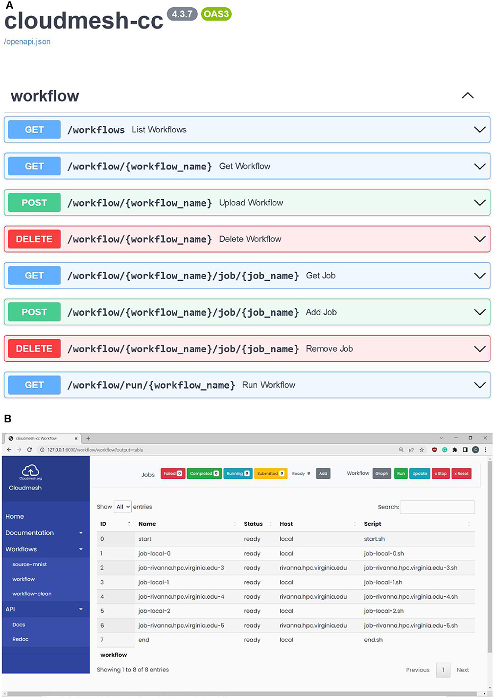
Figure 5. Workflow interfaces. (A) Fast API workflow service. (B) Workflow user interface.

We have tested the framework while running various MNIST application examples, including multilayer perceptron, LSTM, auto-encoder, CNNs and RNNs, and distributed training. A much larger application using earthquake prediction has also been used. Recently, the framework was applied by students to all applications in the MLCommons Applications Working Group. Results of using it outside of the earthquake code are available in von Laszewski et al. (2023).

Figure 5A shows the REST specification and Figure 5B shows the graphical user interface.

3.3.4. Parameterized experiment workflow job generator

In traditional ML workflows, hyperparameter tuning and configuration are key elements in assessing and optimizing the performance of models. However, scaling hyperparameters for highly parallel execution with heterogeneous hardware is complex.

Cloudmesh-ee (von Laszewski, 2023a; von Laszewski et al., 2023) is a hyperparameter and configuration management toolkit designed to address the generation of batch jobs with a consistent and configurable interface based on hyperparameter values across multiple development toolchains. One of its functions is to create batch jobs based on parameterized job specifications and configuration files. Cloudmesh-ee is part of the Cloudmesh toolkit, a set of tools and libraries for managing cloud and HPC resources from the command line, REST interfaces, or graphical user interface (GUIs). Cloudmesh-ee can use a variety of queuing systems and submission commands. Currently, we provide interfaces to simple linux utility for resource management (SLURM), load sharing facility (LSF), and secure shell (ssh).

The architecture of the cloudmesh-ee framework is depicted in Figure 3B.

Cloudmesh-ee differentiates itself from other approaches through its ability to generate a Cartesian product (permutation) of hyperparameters to form independent experiment execution profiles, making it trivial to scale an experiment from one execution to thousands of configurations based on the ranges and their unique combinations. The resulting output provides a generated Slurm or LSF script and a YAML configuration file representing the specific hyperparameters. By managing many highly configurable jobs with cloudmesh-ee, the focus is placed on what hyperparameters to use for experiments and reduce the possibility of human error when running experiments over a range of hyperparameters.

Cloudmesh-ee takes two configuration files. The first is a YAML file that includes all parameters used by the benchmark, including an experiment section that defines the Cartesian product. The second is a Slurm template. From these files, it will create Slurm scripts via the cloudmesh-ee commandline tool while

1. using a unique directory for the experiment,

2. taking a parameter set from the Cartesian product of the experiment parameters,

3. creating from a batch job template an instantiation of the template while replacing all variables from the configuration file and replacing the specific experiment parameters, and

4. creating an instantiation of the configuration file while replacing all experiment parameters with the one for the current experiment.

This is executed for all permutations of the experiment parameters.

An example of a configuration file config.yaml where we iterate over epochs, gpus, and repeat it five times is shown next:

 

      application:

          name: earthquake

  

      data: /scratch/{os.USER}/{application.
          name}

  

      experiment:

          epoch: "1,30,60"

          gpu: "a100,v100"

          repeat: "1,2,3,4,5"

 

An example of a batch script in the cloudmesh template markup follows:

 

      #!/bin/bash

  

      #SBATCH --job-name={experiment.repeat}-{
          application.earthquake}

      #SBATCH --nodes=1

      #SBATCH --gres=gpu:{experiment.gpu}:1

      #SBATCH --time=02:00:00

      #SBATCH --mem=64G

      #SBATCH -o {experiment.gpu}-{application
          .earthquake}/{experiment.repeat}-%j.
          out

      #SBATCH -o {experiment.gpu}-{application
          .earthquake}/{experiment.repeat}-%j.
          err

      #SBATCH --partition=bii-gpu

      #SBATCH --account=bii_dsc_community

  

      export USER_SCRATCH=/scratch/$USER

      cd USER_SCRATCH

      mkdir -p $USER_SCRATCH/{experiment.gpu
          }-{application.earthquake}/%j.out

      nvidia-smi

  

      cms gpu watch --gpu=0 --delay=0.5 --
          dense > outputs/gpu0.log &

  

      python earthquake.py --config config.
          yaml

  

      seff $SLURM_JOB_D

The variables can easily be referred to with a dot notation in the templates. Variables in the YAML file can also be replaced so it is possible to use abbreviations easily and in a consistent fashion in the YAML file as well as in the batch script.

The configuration files and cloudmesh-ee can be configured with parameters so that the files and directories are placed in the right location, and repeatable experiments are created not only on the original machine, but the template can also be easily adapted onto other machines. An example of a variable replacement specification in the YAML file is given for the data value where not only the operating system variable os.USER is replaced, but also the variable {application.name}. Obviously, this is a significant functionality enhancement to a typical YAML file. Multiple values are only possible under the experiment tag, where a variable with multiple values is assigned a string of comma-separated values.

One can choose a number of important parameters as part of the permutation strategy to create different experiments. Common variables are names of graphics cards (if available), memory, file systems used, versions of Python, versions of TensorFlow, epochs, learning rate, and many other important parameters that can influence the benchmark. The reason why we only allow the parameters with variation under experiment is to ensure that there is no confusion with other parameters that may not be modified and instead only represent a single value. However, variables under experiment are also allowed to have just a single value. Another interesting case is the introduction of a repeat parameter, allowing the program to be executed multiple times in order to, for example, support patterns of competition or collaboration while selecting the best values or creating averages.

The final output of cloudmesh-ee is a shell script that contains all jobs that are to be executed with the defined permutations over the parameters. One nice side effect of this is that the jobs in the file can be run in parallel and the queuing system can take over the scheduling of the job following the system-defined queuing policies. However, it may also be possible to create a collaborative group submission, using our earlier introduced collaborative pattern, where multiple users submit a portion of the jobs so that policies restricting the number of jobs per user can be avoided. Furthermore, if access to multiple HPC machines is available, the jobs could be split among the different machines. However, in that case, time measurements may not be a useful parameter to benchmark. However, as in the science group, we are concerned about accuracy, but in addition the combination of a system composed of multiple resources is meaningful.

Our progress with the earthquake benchmark would not have been possible if we did not have cloudmesh-ee to coordinate the many experiments in a consistent fashion. One important aspect is that the management of thousands of jobs that we ran was simplified and the jobs could be created easily while fostering reproducibility. The resulting jobs were run over a month, while each job took many hours to complete.

We have practical experience from multiple teams where coders spent multiple months developing programs and strategies to coordinate their experiment executions; to circumvent this expenditure, the cloudmesh experiment executor generated such permutations within one day on a variety of systems.

Summary of workflow management aspects:

• Challenges:

In benchmarking, we often compare multiple infrastructures and explore many different parameters. This poses the problem of needing to tune and therefore repeat the experiments. Furthermore, we observe that with longer time and larger resource-intensive benchmarks, policies at HPC centers may limit not only the time to execute a benchmark but also the number of jobs that can be executed in parallel.

• Opportunities: We have observed that competitive and collaborative workflow patterns are frequent for benchmarking. We have developed two frameworks that assist in executing benchmarks on multiple HPC systems helping to navigate challenges put in place by center policies, but also allowing the management of large-scale experiment executions through a compute coordinator and an experiment executor that is part of cloudmesh. Together the systems allow workflows to be easily managed addressing job and experiment-related workflows. The systems allow further enhancements and even integration into analytics pipelines using REST interfaces.

4. Benchmark results

In this section, we present some of our concrete benchmark results for the earthquake application while mostly focusing on accuracy while modifying hyperparameters to control the benchmark. In addition to accuracy, we also have provided insights into how the runtime can be predicted to allow scheduling hints for the various batch jobs that we ran. We also have included a brief observation about our experiences with energy monitoring and why it is beneficial. It serves a an example for what students may be able to accomplish. As we will see, the experiment has a significant impact on the hardware configuration that is often overlooked by efforts that do not conduct a holistic benchmark. We start the section by describing the hardware used for the benchmarks.

4.1. Hardware used for this Research

The benchmarks we present in the next sections have been run on a number of compute resources. This includes not only an HPC at UVA but also a desktop, a laptop, and Google Colab to represent different classes of computing resources that students have access to. We used the following resources:

• Rivanna (Univerity of Virginia Research Computing, 2023)—The Rivanna HPC cluster is a system hosted at UVA with 15 different hardware configurations spanning 575 nodes. There exist five different classes of GPUs on these nodes. The Rivanna HPC follows the condominium model and continues to receive additions of nodes and upgrades at various times.

• Google Colab Google Colaboratory (2023)—This a free-to-use interactive computing service offered by Google that provides on-demand access to GPUs and TPUs. Google Colab is designed to be used with ML and data analysis Google Colaboratory (2023). When running with Google Colab, multiple hardware configurations may be provided depending on the instance type. The Pro+ plan allocates an NVIDIA V100 with 53GB of RAM for a GPU configuration. The free plan only offers 32 GB and a P100 GPU.

• Desktop—This is a custom-built desktop with an AMD 5950X processor, 128GB memory, and fast NVMe storage.

• Laptop—This is a store-bought laptop with an AMD 5900HX processor, 16GB memory, and NVMe storage.

The details of the machines are showcased in Table 4.

TABLE 4

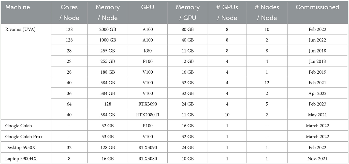
Table 4. Overview of the computing resources.

4.2. Earthquake forecast performance measurements

The original code targets three applications: earthquake forecasting, COVID-19 prediction, and hydrology prediction. We determined that the code could be significantly modified by removing other code unrelated to the earthquake prediction application. This includes removing code for the two additional applications targeting hydrology and COVID-19. Although they use similar DL prediction algorithms, different data and optimization parameters are used. Cloudmesh StopWatch methods were added to obtain code runtime, start, stop, status, and event actions of the different phases of the program. In addition, we augmented the execution of the batch scripts with code that reports energy and temperature using cloudmesh-gpu.

4.2.1. Reproducible experiments

One of the important lessons learned from working within an educational environment is to ensure that experiments can be reproduced early on in the coding process. This not only includes saving the original data in an immutable storage facility but also ensures that the code and parameters of the code are preserved for each experiment. Specifically, we ensure this preservation by using configuration files and Singularity containers.

Code used during a development phase should not be used especially if they are developed with Jupyter Python notebooks that could contain an implicit hidden state that causes side effects. Hence, the benchmark must be saved in a clean fashion so that no other result-impacting effects occur.

4.2.2. Measuring runtime

As the code requires a significant amount of time to execute, we first had to estimate the projected runtime for a number of epochs. Hence, after the code augmentations, we obtained for a small number of epochs (2, 10) the runtime and projected the runtime for various systems from these values. As our ML code performs similarly to linear growth when increasing epochs, it was possible to fairly accurately predict the performance while larger numbers of epochs improved the prediction accuracy. As we need to reserve resources on any shared compute resource if it is an HPC system, such runtime predictions are extremely important to accurately estimate to preserve allocation usage. For completeness and to verify the linear behavior, we also executed performance experiments with a larger number of epochs.

We also wished to estimate how much time is spent on the GPU versus the rest of the program. This allowed us to predict the runtime more accurately, and what impact setting up the application has on the runtime. Figure 6A shows the time measured for a two-epoch case for modeling prediction and the rest of the application. The bars in the histogram are divided while the top part indicates the model prediction for two epochs, and the bottom part is the rest of the application's runtime. These numbers can then be used to generate predictions while varying the epoch numbers as multipliers and using the benchmark data for the particular GPU used.

FIGURE 6

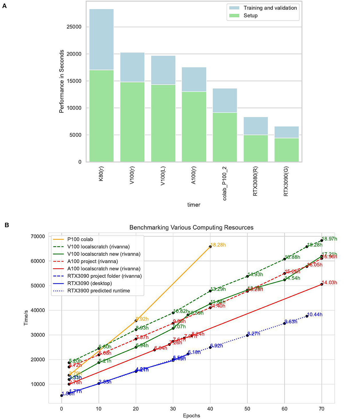
Figure 6. Performance time measurements. GPU. (A) Time of the best fit in seconds of performance measurements while using 2 epochs on various systems with different GPUs. The lower portion (green) of each bar represents the setup time, while the upper portion (blue) represents the training and prediction time. The setup time is constant throughout the experiments, while with an increasing number of epochs the training and prediction time will dominate. (B) Time performance benchmark for various GPU cards on different systems and variations of epochs.

Figure 6B indicates the time spent in the application. To produce this graph, we ran the application (as previously mentioned) while varying the epochs between 2 and 70 to obtain the runtime. The total runtime for various configurations with different GPUs and file systems (where choices for the file system existed) is shown in Figure 6B. This experiment was also run on the desktop using an AMD 5950X with an RTX3090 and 128 GB of memory while data were located on an NVMe. The data on the HPC system were initially located on an NSF storage system (indicated by the name project for the /project or scratch for the /scratch file system). As we see, the desktop with an RTX3090 is significantly faster than the HPC compute node equipped with any other GPU (including an A100), which was a surprise not only to the team but also to the research staff. To quantify this result, we enumerate the results for a two-epoch case in Table 5. To our surprise, we found that the RTX3090 machine was almost 2.67 times better than the HPC machine with an A100.

TABLE 5

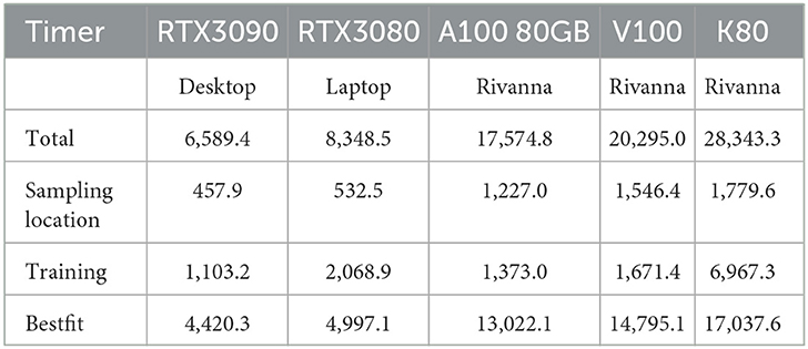
Table 5. Runtime of the two-epoch case in seconds.

The same desktop computer also significantly outperformed benchmarks conducted on Google Colab. We discovered that Google Colab, although suitable for small epoch runs, quickly deteriorated with an increasing number of epochs due to the older GPUs with Google Colab's present hardware availability.

The reason why the desktop performed so well is that it had up-to-date, fast memory and that the data were hosted on fast NVMe storage. As the earthquake application uses many data requests, fast IO makes a big difference. This performance analysis has guided us to propose changes to the HPC machine, which are in the process of being implemented. Future expansions of the HPC machine include a 28TB upgrade to the GPUs accessible NVMe storage. Our benchmark is a good use case for motivating this update.

Based on these findings, we influenced a change in the architecture of the HPC server nodes to add a file system with NVMe storage on it. However, as our measurements show, the desktop significantly outperformed the HPC system; additional changes will need to take place even after this upgrade while updating servers to the newest generation of NVIDIA hardware. This upgrade will focus on increasing the bandwidth of data transfers between the file system and the GPU so that the GPU can be properly utilized. We anticipate that such a system will become available to us in the fall of 2023.

However, for our experiments, we were only running the desktop for up to 33 epochs, and the dotted line includes our prediction of the runtime based on our previous values. The reason for this is that during our experiments, we ran out of memory on the desktop to produce the visualization that is part of the overall program. The insight we gained is that one must ensure that the data feed to the GPU can keep up with the GPU's performance. It is not sufficient to add GPUs to a server that may not have adequately fast file systems, memory, or processors.

For our next experiments, we need to distinguish the different phases of the application in more detail. We have augmented the code with timers that return information about the following phases:

• Total. This shows the total runtime of the application and includes all additional phases mentioned here.

• Initialize. Time to initialize all variables and data and split data into train, validation, and test.

• Sampling locations. Time to sample time-series data into 2-week batches.

• Training or Model Fit. Time to train the model and determine and save the best fit from all epochs.

• Bestfit or Bestfit Prediction. Time to find the best-fit model to calculate predictions.

• Visualize. Time to organize all predictions into an organized structure so the MSE and NNSE can be calculated, and accuracy graphs can be identified.

• Final Plots. Time to gather data collected during model runtime and move to a permanent directory and process plots and graphs from data. Then, clean up data and close all unneeded processes.

4.2.3. Accuracy performance benchmark

Since MLCommons Science Working Group's focus is improving an application's accuracy, this section reports on the accuracy of the earthquake application.

We observe that application loss for validation and training intersects at the 30–33 epoch value (see Figure 7). We have also tested larger epoch runs up to 90 epochs. Our best accuracy values are found at our 90 epoch runs.

FIGURE 7

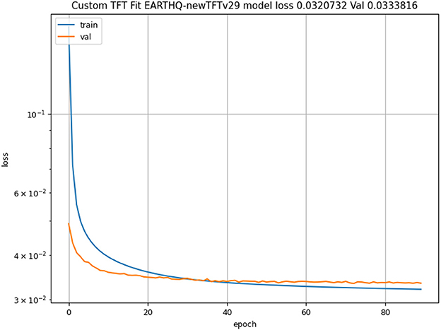
Figure 7. Loss comparison between training and validation data. TFT, temporal fusion transformer.

However, generally, we can say that at the intersection point, the model's performance on the validation set starts to degrade while its performance on the training set continues to improve. Hence, the model is fitting the training data too well while at the same time not being able to generalize our validation data leading to overfitting. As the training loss continues to decrease with an increased number of epochs after the intersection point, the model has become too complex and captures noise in the training data. This analysis provides an excellent opportunity for future benchmarking activities to deal with overfitting while considering techniques such as early stopping, regularization, the reduction of the model complexity, reorganization of the data, cross-validation, and additional hyperparameter tuning.

4.2.4. Prediction parameters for input and prediction data

For the rest of the experiments, we have chosen different input and output vectors that are used as hyperparameters or prediction parameters. In the subsequent benchmark results, these groupings of data are used as part of the training to optimize their associated accuracy values.

The data is grouped into 2 week periods. The model steps through each of these 2-week groupings and uses training data up to 1 year into the past from the current 2-week grouping. The model uses up to 1 year, ≤26 data points, before the current 2-week grouping run on the model as training data. For example, if the model is taking the first 2 weeks of January 2000, it would take ≤26 2-week groupings before that point as training data, so all 1999 data would be 26 data points. Then it repeats this method with the next 2-week period in sequence, which would be the 2-week grouping of weeks 3 and 4 of January 2000, and the training data would be the previous 26 2-week groupings from that point or the first 2 weeks of January 2000 and the previous 25 2-weeks groupings of 1999, all of 1999 data except first 2 weeks of 1999. It repeats this until all 2-week groupings are used in the model.

We have introduced a convenient nomenclature for the data input. This nomenclature uses the following rules that are applied to control how parameters are used as input and output data:

• All data were grouped into 2-week periods.

• The term Now indicates the most recent rolling sequential date from the data set; the Term #M or #Y corresponds to the number of months or years prior to Now to use when sampling the data.

• An optional moving window is applied based on a range of 2-week grouping from the specified time frame. For example, 2wk+26AVG is an abbreviation for performing the calculation over 26 groupings. When not specified, only one observation is collected.

Applying these rules, a range of values is notated by first specifying a 2-week grouping and then the number of observations to include. For example, a value of 1Y 2wk+26AVG is 1 year from the 2-week grouping the model is currently on; the rolling training group is run on the data set, taking 26 2-week groupings from that date. Another example is the value of 1 Year Back, which is a single 2-week occurrence 1 year ago from the rolling training group. Another example is Now 2wk+7AVG, which is 7 2-week groups from the rolling training group.

4.2.5. Competitive accuracy benchmarks

Next, we summarize the competitive accuracy benchmark where we use the nomenclature for the input and output hyperparameters defining the time period used for the training and validation. To simplify our presentation, we have decided to use epoch values 2, 30, 70, and 90 for this article's experiments. We took all results and sorted them for training and validation separately by the accuracy values. This leads to a ranking of the experiments by accuracy. In Table 6, we present the top 20 accuracy values, while in Figures 8A, B, we created a histogram showcasing how many accuracy values fall into a certain bucket over all experiments for training and validation.

TABLE 6

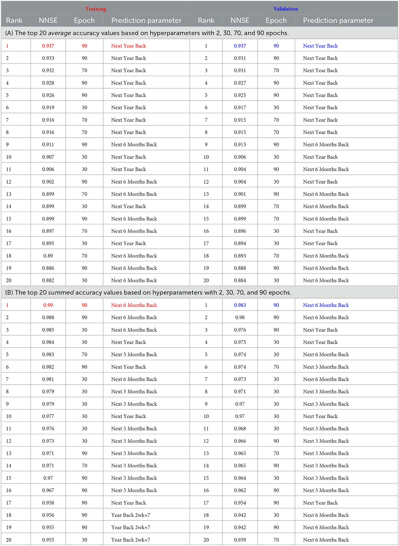
Table 6. Ranking of the top 20 accuracy values.

FIGURE 8

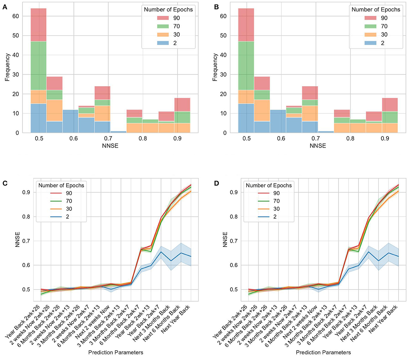
Figure 8. Evaluation of the normalized Nash–Sutcliffe efficiency average accuracy for epochs 2, 30, 70, and 90. (A) Histogram of the average accuracy values for every epoch over all experiments for training. (B) Histogram of the average accuracy values for every epoch over all experiments for validation. (C) Average accuracy values over all experiments for training sorted by best training values. (D) Average accuracy values over all experiments for validation sorted by best validation values.

From the table, we see that we achieve the best results using the parameters (epoch=90, Next Year Back). From the histogram, we see that the best results stem mostly from 90 epochs.

Hence, although we are mostly interested in identifying the best accuracy value, it is also advantageous to reflect that data place the 90-epoch case above the other values, generally leading to better results (see Figure 8A) for training.

To identify more details about the most accurate results and the prediction parameters (hyperparameters) used to create them, we have plotted the accuracy values in Figures 8C, D.

Here we have sorted the hyperparameters by the accuracy values for the validation where the best accuracy for each hyperparameter is identified and sorted in increasing fashion. We have then taken the same order of the hyperparameters and applied the order to the training. The diagrams include the minimum and maximum accuracy values for a hyperparameter found using 2, 30, 70, and 90 as epochs, while the experiment has been repeated five times. The average for each accuracy for a given epoch is shown. Additionally, the confidence interval for each epoch is added as a highlighted area.

The best average value for the hyperparameter Next Year Back is 0.937 for training and 0.937 for validation (see Table 6).

Not only did we find that the best epoch for accuracy is 90, but the best hyperparameters are also Next Year Back for average NNSE and Next 6 Months Back for summed NNSE, meaning that according to our nomenclature, the previous year and 6 months of observation readings from the current rolling training group is used as training data in support of our model.

Although we see, on average, better accuracy results with 30 epochs, the best accuracy values we still have seen with 90 epochs. This indicates that we have a higher variation of the results in the 90-epoch case. However, as we are competing for the best value and not the average value, this variation has an advantage as we do not as easily get stuck in a local minima.

One other observation we can make is that the training NNSE value is higher than that of validation. This leads us to believe that the input data may be incomplete to train the model more accurately or that the input data need to be differently structured to have a higher validation accuracy value. Hence, although this work is a good starting point, we believe there is significant room for improvement.

We can make similar observations when looking at the summed accuracy values. However, here we see that more of the best accuracy values are retrieved when using 90 epochs. We see in the average and summed accuracy that the best 20 values have been created with the prediction parameters of Next Year Back, Next 6 Month Back, and Next 3 Month Back. The average shows a more uniform distribution of these parameters in the top 20 than the summed NNSE values (see Figure 9).

FIGURE 9

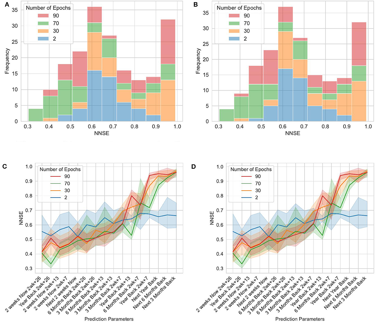
Figure 9. Evaluation of the normalized Nash–Sutcliffe efficiency summed accuracy for epochs 2, 30, 70, and 90. (A) Histogram of the summed accuracy values for every epoch over all experiments for training. (B) Histogram of the summed accuracy values for every epoch over all experiments for validation. (C) Summed accuracy values over all experiments for training sorted by best training values. (D) Summed accuracy values over all experiments for validation sorted by best validation values.

As we can see further educational opportunities can be derived from analyzing different prediction parameters and different input data distributions.

Summary application benchmark:

• Challenges: Today's students have a limited understanding of HPC resources. This not only includes the CPU and GPU but also network and storage resources. How to use these resources leads to optimizations while efficiently using the hardware. While in some educational activities, students only gain an understanding of a single model, application benchmarks require measuring different combinations of input and output data as well as various models. This is important as in many cases the best combination has to be found.

• Opportunities: We identified while providing students with a detailed understanding of the hardware optimizations by the students to utilize them have been found. Furthermore, introducing a “leader-board” of different models and applications using a variety of input and output options provides the students with a more general approach to identifying good results. The students understand that different parameters for benchmarks not only include the hyperparameters of a DL algorithm but also the data used and the hardware. Many topics can be added to this such as identifying overfitting and how to prevent it, which is beyond the scope of this article.

4.2.6. Energy

When proposing research activities with students, discussions about energy are a highly relevant and engaging topic in today's world due to the pressing issue of climate change. With increased extreme weather, students become more aware of the necessity for ML applications that can help increase understanding and analysis of such weather. Additionally, students understand the need for cautious and responsible resource usage, with energy consumption being a prime example that can be reasonably well measured when using electronic devices such as GPUs. In our interactions with students, we have observed that they are not merely interested in finding out the best or most efficient results but, once made aware of energy consumption measurement, that they also want to understand more about how to measure it and how it impacts different algorithms and use of different compute resources. To cater to this curiosity, we have developed an easy-to-use energy trace component that can be started in parallel to our performance experiments, called cloudmesh-gpu. It returns the energy at predefined time intervals and contains examples on how to read and plot the data, as well as calculate a traced energy consumption provided during the traced events.

We have actively observed that students students changed their attitude from “I do not care how long the experiment runs as I do not have to pay for it” to “I should care for how long it runs as it has a direct impact on the energy consumption, which may adversely impact the environment I am living in.” Such discussions are also related to one aspect of an ethics discussion of the use of AI. What is the impact on our environment when using AI in general? We certainly do not provide an answer to this question, but we use this curiosity to start students to think more globally. For example, one could ask how much energy is consumed by students learning AI with a standard example that has been run abundantly, such as done in regular AI classes with, for example, MNIST. Could we not replace it with different benchmarks that relate directly to other applications that have a more direct impact on the well-being of humans such as earthquakes? However, we recognize that MNIST and character recognition in general are useful to support the blind, for example. Thus, bringing such examples into the research experience for students is an important aspect with energy being one metric to consider. Furthermore, it indirectly has an impact on the operational cost of a center and future improvements could associate the energy cost per kWh for particular regions and time of the day to contrast regional differences in running such applications.

Now that we have introduced why energy is a vital topic to be included in benchmarks, we provide a more detailed discussion about its technical aspects and how we applied it in our analysis.

One aspect of energy consumption that is most often discussed is cost. Energy consumption has become an important factor in the evaluation of computing centers due to the high costs associated with running them on a large scale. This not only includes common compute center-based metrics such as power usage effectiveness but also the measurement of application-oriented energy consumption. Such application-oriented comparisons have led to a ranking of the most energy-efficient supercomputers as detailed in the Green500 list (Feng et al., 2007). In such comparisons, the metric Energy Efficiency is used and derived by the GFlops/watts value. Just like TOP500, this benchmark is based on Linpack performance measurements (Top500, 2023). However, it is important to also consider other applications when measuring energy consumption. Such applications may consist of many different phases and may not perform at the maximum potential performance of the available hardware, or the available hardware may project a bottleneck for the performance.

To measure the algorithm's energy consumption, we need to augment the application in such a way that we can monitor energy use over the lifetime of the application execution. For this, we have developed a simple-to-use energy trace program to monitor and predict our energy uses called cloudmesh-gpu as introduced in Section 3. We used for our initial experiments data hosted on an NFS file system in the data center as localscratch was not available at the time.

With this program, we can create energy traces of the GPU. An energy trace is a sample of energy measurements periodically taken over time of the GPU. The period of the measurements can be decreased to increase the accuracy of the energy measurements over time. Our presentation here only includes measurements of the GPU and does not include the measurement of the servers, file system, or network energy consumption, as our focus for this study is the impact on GPUs and to see if they are efficiently used.

In our case, we chose to measure the GPU energy used every second leading to an energy trace that we term $E_{\Delta t=1s}^T(GPU)$. Such traces can be applied to the application running with different hyperparameters. To showcase the drastically different energy traces, we have limited our discussion to running applications on different GPUs (A100 and V100) and different epochs (2, 30, and 70). These traces are depicted in Figures 10A–F. To better showcase the impact of the different phases of the application, we have augmented the traces with different colors for the different phases of the application. We distinguish the phases called Initialize, Training, Best Fit Prediction, Visualize, and Final plots. The meaning of these phases has been explained in Section 4.2.2 and we have used different colors for the phases in Figure 10 to distinguish them better.

FIGURE 10

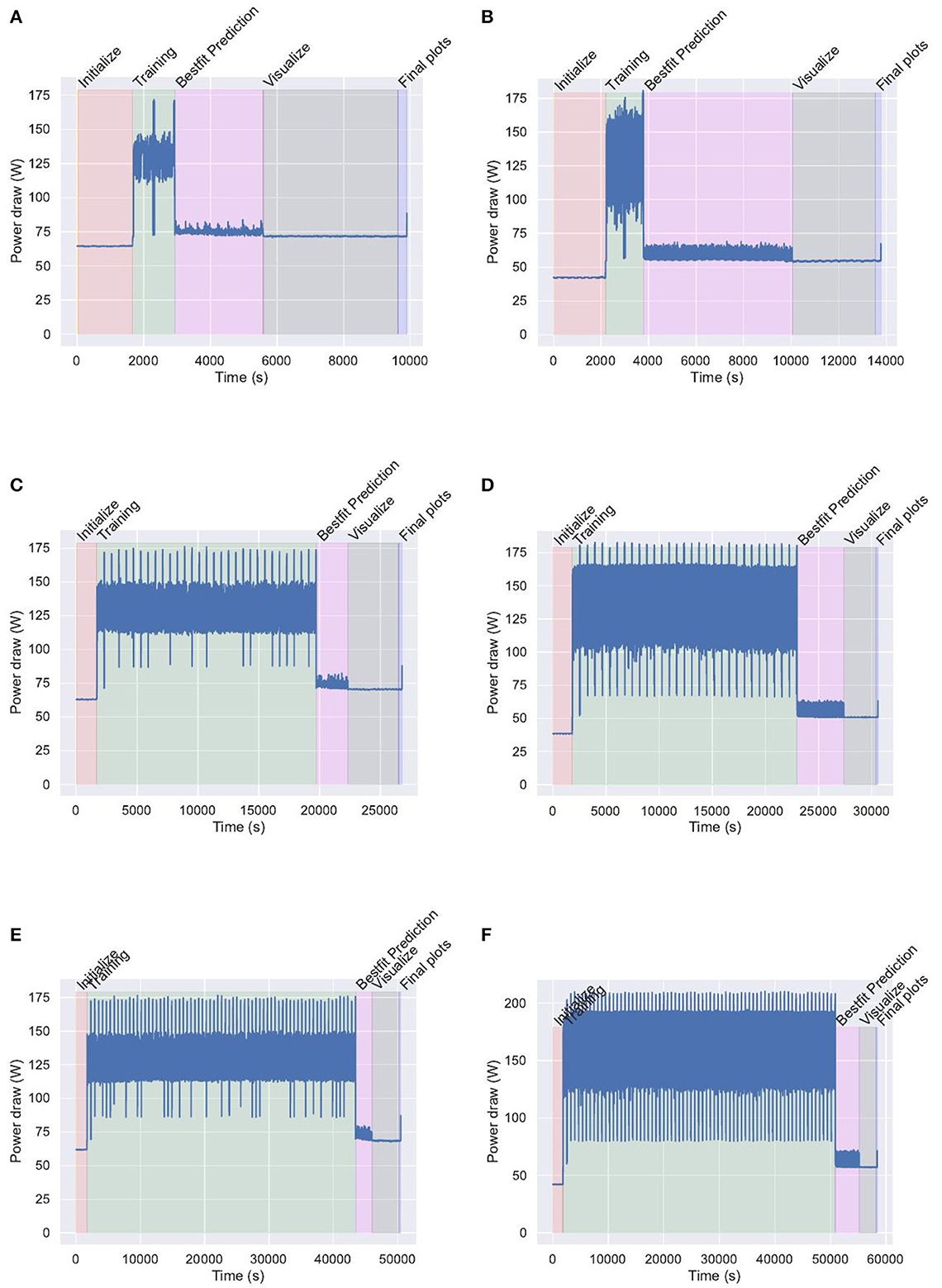
Figure 10. Energy traces for training and validation for epochs 2 (A, B), 30 (C, D), and 70 (E, F). The sampling rate is 1s. (A) A100 energy trace $E_{\Delta t=1s}^T(GPU)$ for 2 epochs training and validation. (B) V100 energy trace $E_{\Delta t=1s}^T(GPU)$ for 2 epochs training and validation. (C) A100 energy trace $E_{\Delta t=1s}^T(GPU)$ for 30 epochs training and validation. (D) V100 energy trace $E_{\Delta t=1s}^T(GPU)$ for 30 epochs training and validation. (E) A100 energy trace $E_{\Delta t=1s}^T(GPU)$ for 70 epochs training and validation. (F) V100 energy trace $E_{\Delta t=1s}^T(GPU)$ for 70 epochs training and validation.

An important observation for the training phase (colored in green) that the energy values of the GPU are significantly higher than in the rest of the application, indicating a much higher utilization of the GPU during that phase.

The other phases dealing with data reparation only show a modest use of the GPU. We have measured the energy consumption between different GPUs. When looking at the energy traces in Figure 10, showing the differences between A100 and the V100 GPUs, we note that the time on the abscissa is significantly larger for the V100. Hence, overall energy consumption per second will be significantly larger. The fluctuations of the energy in the training phase can be explained through the various repeated processes that exist within the training of the DL application.

To compare the energy values between different GPUs such as A100, V100, and P100, we can calculate the energy trace consumption, defined as the sum of all energy values in an energy trace $E_C^T\sum E_{\Delta t=1s}^T(GPU)$ applied to a hyperparameter such as the epoch. We can then calculate the energy trace consumption per epoch which we plotted in Figure 11A. The time with higher epoch numbers is dominated by the training time as seen in Figure 10. Hence, the energy per epoch for lower numbers of epochs will be small, while for larger numbers, the energy per epoch will be higher. However, they will not change much with higher numbers of epochs as demonstrated in Figure 11A. We also see that the K80 uses significantly higher energy than the other GPUs, with the A100 performing best. For K80 and 70 epochs, we could not obtain a value as it was outside the allowed time to run applications on the supercomputer defined by the center's policy. We also see that the standard deviation for the kWh/Epoch value becomes smaller with an increasing number of epochs.

FIGURE 11

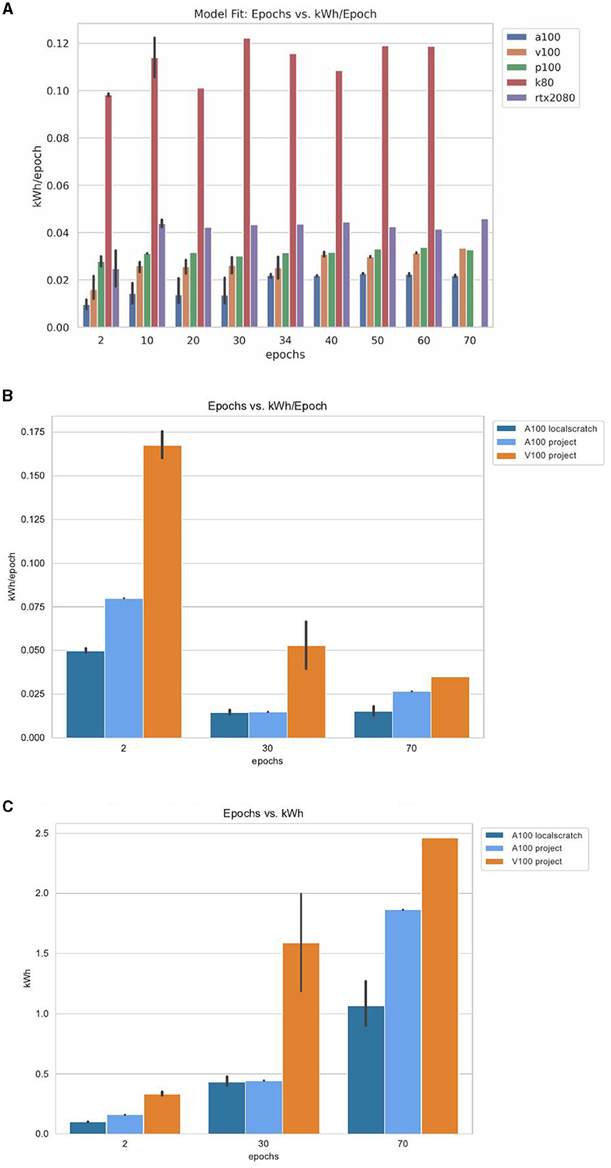
Figure 11. Averaged energy consumption of various GPUs targeting a 1 second data sampling rate. The recorded values in (A) and all V100 reported are produced with an NFS-mounted file system. The data for A100 in (B, C) are using localscratch's NVMe storage. GPU, graphical user interface; NFS, network file system; NVMe, non-volatile memory express.

This means that the power usage of GPUs is generally constant when training our benchmark model and could be used for energy prediction.

In Figure 11B, we also depicted the energy trace per epoch. However, in contrast to Figure 11A that was created using the data on an NFS storage device, we included here the values obtained for data hosted on a localscratch file system and the project file system. While the localscratch uses NVMe storage, the project file system is hosted on a shared GPFS storage server. Accessing the data from there takes more time and hence more energy is used during the benchmark per epoch.

Hence, it offers a clear insight into how a file system can negatively impact the energy as the runtime is enhanced and the GPU time to cool down or adjust for reducing the energy is too small to have an impact.

Additionally in Figure 11C, we summarize the total GPU energy consumption of the traces from the complete execution of the benchmark notebook depicting measures from the phases Initialize, Training, Bestfit Prediction, Visualize, and Final Plots. This graph is important, as it shows the impacts of the energy usage of the GPU throughout the runtime and when compared to the plots in Figures 11A, B, outlier events, such as a potential interaction from other users sharing the benchmark infrastructure can be identified.

Such phases and making clear that GPUs may not be used in some of them could also lead to a rewrite of the code to also use GPUs in these phases.

Students now have easy means to measure and improve through algorithmic means the energy consumption in the various phases, but also the overall consumption for a scientific application. External data (ene, 2020) can be used to obtain information about the cost of such calculations. However, in many cases, these data need to be augmented as data centers may have special pricing for energy consumption. Thus, it is very useful to also consider greenhouse gas emissions instead (Oar, 2023). In our future work, we like to integrate such data into the energy monitor we have currently.

Summary energy benchmarks:

• Challenges: MLCommons has not yet integrated a comprehensive energy benchmark. Tools to easily gather energy information are unknown to the students and often not accessible.

• Opportunities: We have discovered that energy as a topic attracts a number of students and increases interest in applications. We have made simple tools as part of cloudmesh available to create energy traces and display their result. These tools were not only used by the students but also to demonstrate that we used the indeed GPUs, as our initial benchmark showed they were very slow due to the use of a recommended parallel file system. It showed to us that we need to spend more time in future activities on energy monitoring in general.

5. Discussion

This article summarizes a large body of work that addresses multiple aspects of ML benchmarking. We identified that benchmarking can lead to a significant educational contribution to students and researchers. We identified that not only is software carpentry needed but also benchmark carpentry, an effort that we termed in conjunction with the MLCommons Science Working Group. We have demonstrated that students are capable of conducting sophisticated benchmarks while dealing with complex system-related infrastructure and working with policies set by HPC compute centers that deal with fair resource management. To deal with this, we have also developed a compute coordination and workflow management system in two components called cloudmesh-ee and cloudmesh-cc that allow benchmark jobs to be automatically generated from hyperparameter permutations. It also allows us to coordinate such benchmarks on different machines. We have identified the patterns of selection, cooperation, and competition which are part of a benchmark workflow. Furthermore, we have improved the original benchmark code in many aspects. To simplify benchmarking, we also developed an easy-to-use StopWatch that in contrast to the mllog library used by MLCommons is simpler and is immediately humanly readable. Finally, our benchmarks had a significant impact on the operation and accessibility of software in the educational cluster we used. Plans for new file system management and updated compute nodes excite us to conduct more such studies. We intend to submit our results to the MLCommons Science Working Groups as earthquake forecasting is one of their benchmark codes and efforts. We have outlined opportunities and challenges how MLCommons benchmarks can be integrated in AI classes and focusing on DL.

6. Nomenclature

6.1. Resource Identification Initiative

Organization: RRID:SCR_011743

Data availability statement

The datasets presented in this study can be found in online repositories. The names of the repository/repositories and accession number(s) can be found in the article/supplementary material. All data is available at https://github.com/laszewsk/mlcommons-data-earthquake.

Author contributions

GL has modified and augmented the earthquake code to include the ability to execute hyperparameters. JPF has contributed to various aspects of the workflow component of the article and a number of executions and evaluations of experiment runs. RK has helped together with GL in the implementation of cloudmesh-sbatch and the porting of the effort to the UVA machine. GL developed an improved version of cloudmesh-sbatch that is now distributed under the name cloudmesh-ee. GF facilitates the interactions with the MLCommons Science Working Group as a group leader of that effort. TB and JK participated in an earlier phase of the project that ported and improved an earlier version of the code while adding timers and the energy monitor developed by GL. JF was enabling the students RK, TB, and JK to participate in this project and provided administrative supervision to meet the class expectations and requirements needed for their participation. All authors contributed to the article and approved the submitted version.

Funding

Work was in part funded by the NSF CyberTraining: CIC: CyberTraining for Students and Technologies from Generation Z with the award numbers 1829704 and 2200409, the NSF CINES Grant #2210266, and NIST 60NANB21D151T. The work was also funded by the Department of Energy under the grant Award No. DE-SC0023452. The work was conducted at the Biocomplexity Institute and Initiative at the University of Virginia.

Acknowledgments

We like to thank TB and JK for their initial contributions during the capstone project while focusing on executing initial runs of the code and experimenting with modifications to the code including logging. Please note that since this team finished their work, significant improvements have been made by the GL and JPF. We also thank the reviewers for their valuable comments to improve the paper.

Conflict of interest

The authors declare that the research was conducted in the absence of any commercial or financial relationships that could be construed as a potential conflict of interest.

The author GF declared that they were an editorial board member of Frontiers at the time of submission. This had no impact on the peer review process and the final decision.

Publisher's note

All claims expressed in this article are solely those of the authors and do not necessarily represent those of their affiliated organizations, or those of the publisher, the editors and the reviewers. Any product that may be evaluated in this article, or claim that may be made by its manufacturer, is not guaranteed or endorsed by the publisher.

References

Claesen, M., and De Moor, B. (2015). “Hyperparameter search in machine learning,” in MIC 2015: The XI Metaheuristics International Conference in Agadir. Morocco. arXiv. Available online at: https://arxiv.org/abs/arXiv:1502.02127

Google Scholar

Dongarra, J. J., Meuer, H. W., Strohmaier, E., and Simon, H. D. (1997). TOP 500 supercomputer sites. Supercomputer 13, 89–111.

Google Scholar

Feng, W., Cameron, K. W., and Snavely, A. (2007). “The Green500: a ranking of the most energy-efficient supercomputers,” in Proceedings of the 2007 ACM/IEEE Conference on Supercomputing (SC '07) (ACM), 63.

Google Scholar

Fincher, S. A., and Robins, A. V. (2019). “Systems software and technology,” in Cambridge Handbooks in Psychology. Cambridge: Cambridge University Press, 637–706.

Google Scholar

Fleischer, J. P., von Laszewski, G., Theran, C., and Parra Bautista, Y. J. (2022). Time series analysis of cryptocurrency prices using long short-term memory. Algorithms 15, 7. doi: 10.3390/a15070230

CrossRef Full Text | Google Scholar

Fox, G., Rundle, J., Donnellan, A., and Feng, B. (2022). Earthquake Nowcasting with Deep Learning. Geohazards 3, 199. doi: 10.3390/geohazards3020011

CrossRef Full Text | Google Scholar

Fox, G. C., von Laszewski, G., Knuuti, R., Butler, T., and Kolesar, J. (2023). “MLCommons science benchmark earthquake code,” in GitHub. Available online at: https://github.com/laszewsk/mlcommons/tree/main/benchmarks/earthquake (accessed April 13, 2023).

Google Scholar

Google Colaboratory (2023). “Google Colab FAQ,” in Web Page. Available online at: https://research.google.com/colaboratory/faq.html (accessed April 13, 2023).

Google Scholar

Königstorfer, F., and Thalmann, S. (2022). AI documentation: a path to accountability. J. Responsible Innov. 11, 100043. doi: 10.1016/j.jrt.2022.100043

CrossRef Full Text | Google Scholar

Kovtaniuk, M. S. (2022). “Online compiler «replit»usage during the study of the programming discipline,” in Information Technologies And Management In Higher Education And Sciences. Latvia: Baltija Publishing.

Google Scholar

Lim, B., Arık, S. Ö, Loeff, N., and Pfister, T. (2021). Temporal fusion transformers for interpretable multi-horizon time series forecasting. Int. J. Forecast. 37, 1748–1764. doi: 10.1016/j.ijforecast.2021.03.012

CrossRef Full Text | Google Scholar

Mathuriya, A., Bard, D., Mendygral, P., Meadows, L., Arnemann, J., Shao, L., et al. (2018). CosmoFlow: using deep learning to learn the universe at scale. arXiv. arXiv:1808.04728.

Google Scholar

Mattson, P., Cheng, C., Coleman, C., Diamos, G., Micikevicius, P., Patterson, D., et al. (2019). MLPerf training benchmark. arXiv. arXiv:1910.01500.

Google Scholar

MLCommons (2023). “Machine learning innovation to benefit everyone,” in Web Page. Available online at: https://mlcommons.org/ (accessed April 13, 2023).

Google Scholar

Nash, J., and Sutcliffe, J. (1970). River flow forecasting through conceptual models part i-a discussion of principles. J. Hydrol. 10, 282–290. doi: 10.1016/0022-1694(70)90255-6

CrossRef Full Text | Google Scholar

Norem, J. (2023). “Windows 11 Gains Market Share but Windows 10 Still Leads by a Mile,” in ExtremeTech. (accessed July 25, 2023).

Google Scholar

Oar (2023). Greenhouse Gas Equivalencies Calculator. Washington, D.C.: US EPA.

Google Scholar

Open OnDemand (2023). Open On Demand | Research Computing. Deployment at University of Virginia based on Hudak et al., (2018). Open OnDemand: A web-based client portal for HPC centers. J. Open Source Softw. 3, 622. doi: 10.21105/joss.00622

CrossRef Full Text | Google Scholar

Papermill (2020). Parameterize, Execute, and Analyze Jupyter Notebooks. Zenodo.

Google Scholar

Raibulet, C., and Fontana, F. A. (2018). Collaborative and teamwork software development in an undergraduate software engineering course. J. Syst. Softw. 144, 409–422. doi: 10.1016/j.jss.2018.07.010

CrossRef Full Text | Google Scholar

Shapiro, R. B., Fiebrink, R., and Norvig, P. (2018). How machine learning impacts the undergraduate computing curriculum. Commun. ACM 61, 27–29. doi: 10.1145/3277567

CrossRef Full Text | Google Scholar

SLURM (2003). “Homepage,” in Web Page. Available online at: https://slurm.schedmd.com (accessed April 13, 2023).

Google Scholar

Tan, J., Chen, Y., and Jiao, S. (2023). Visual Studio Code in Introductory Computer Science Course: An Experience Report. arXiv. Available online at: https://arxiv.org/abs/2303.10174

Google Scholar

The PEP Editors (2023). PEP 8 –Style Guide for Python Code |. Available online at: peps.python.org (accessed 6 Sep, 2023).

Google Scholar

Thiyagalingam, J., von Laszewski, G., Yin, J., Emani, M., Papay, J., Barrett, G., et al. (2022). “AI benchmarking for science: efforts from the MLCommons science working group,” in High Performance Computing. ISC High Performance 2022 International Workshops, eds. H., Anzt, A., Bienz, P., Luszczek, and M., Baboulin. Cham: Springer International Publishing, 47–64.

Google Scholar

Top500 (2023). “Homepage,” in Web Page. Available online at: https://www.top500.org/ (accessed April 13, 2023).

Google Scholar

Tovar, B., Bockelman, B., Hildreth, M., Lannon, K., and Thain, D. (2021). “Harnessing hpc resources for cms jobs using a virtual private network,” in EPJ Web of Conferences, 251. Les Ulis, France: EDP Sciences. doi: 10.1051/epjconf/202125102032

CrossRef Full Text | Google Scholar

U.S. Bureau of Labor Statistics (2020). Average Energy Prices for the United States, Regions, Census Divisions, and Selected Metropolitan Areas. Illinois: Midwest Information Office: U.S. Bureau of Labor Statistics.

Google Scholar

Univerity of Virginia Research Computing (2023). “Rivanna,” in Web Page. Available online at: https://www.rc.virginia.edu/userinfo/rivanna/overview (accessed April 13, 2023).

Google Scholar

von Laszewski, G. (2005). “Java CoG Kit Workflow Concepts for Scientific Experiments,” in Technical Report P1259. Argonne, IL: Argonne National Laboratory. Available online at: https://www.mcs.anl.gov/uploads/cels/papers/P1259.pdf (accessed October 3, 2023).

Google Scholar

von Laszewski, G. (2022a). “Cloudmesh Common StopWatch,” in GitHub. Available online at: https://github.com/cloudmesh/cloudmesh-common/blob/main/cloudmesh/common/StopWatch.py (accessed April 13, 2023).

Google Scholar

von Laszewski, G. (2022b). “Cloudmesh GPU monitor,” in GitHub. Available online at: https://github.com/cloudmesh/cloudmesh-gpu (accessed April 13, 2023).

Google Scholar

von Laszewski, G. (2023a). Cloudmesh Experiement Executor. Available online at: https://github.com/cloudmesh/cloudmesh-ee (accessed September 8, 2023).

Google Scholar

von Laszewski, G. (2023b). MLCommons Earthquake Data. Available online at: https://github.com/laszewsk/mlcommons-data-earthquake (accessed April 13, 2023).

Google Scholar

von Laszewski, G., Fleischer, J. P., and Fox, G. C. (2022). Hybrid reusable computational analytics workflow management with cloudmesh. Technical report. arXiv. arXiv:2210.16941.

Google Scholar

von Laszewski, G., Gawor, J., Pena, C., and Foster, I. (2002). “InfoGram: a grid service that supports both information queries and job execution,” in Proceedings 11th IEEE International Symposium on High Performance Distributed Computing, 333–342.

Google Scholar

von Laszewski, G., Hategan, M., and Kodeboyina, D. (2007). Java CoG Kit Workflow. London: Springer London, 340–356.

Google Scholar

von Laszewski, G. J. P., Fleischer, J., Fox, G. C., Papay, J., Jackson, S., et al. (2023). “Templated hybrid reusable computational analytics workflow management with cloudmesh, applied to the deep learning mlcommons cloudmask application,” in Second Workshop on Reproducible Workflows, Data, and Security (ReWorDS 2022). Limassol, Cyprus: eScience'23.

Google Scholar

Wilson, G., Aruliah, D. A., Brown, C. T., Hong, N. P. C., Davis, M., Guy, R. T., et al. (2014). Best practices for scientific computing. PLoS Biol. 12, e1001745. doi: 10.1371/journal.pbio.1001745

CrossRef Full Text | Google Scholar

Zeidmane, A., and Cernajeva, S. (2011). “Interdisciplinary approach in engineering education,” in 2011 IEEE Global Engineering Education Conference (EDUCON), 1096–1101.

Google Scholar

Zou, Z., Zhang, Y., Li, J., Hei, X., Du, Y., and Wu, D. (2017). “Easyhpc: An online programming platform for learning high performance computing,” in 2017 IEEE 6th International Conference on Teaching, Assessment, and Learning for Engineering (TALE). Hong Kong: IEEE, 432–435.

Google Scholar