The fast and the capacious: memory-efficient multi-GPU accelerated explicit state space exploration with GPUexplore 3.0

1 Introduction

Major advances in computation increasingly need to be obtained via parallel software as Moore's Law comes to an end (Leiserson et al., 2020). In the last decade, GPUs have been successfully applied to accelerate various computations relevant for model checking, such as probability computations for probabilistic model checking (Bošnački et al., 2011; Wijs and Bošnački, 2012; Khan et al., 2021), counter-example construction (Wu et al., 2014), state space decomposition (Wijs et al., 2016a), parameter synthesis for stochastic systems (Češka et al., 2016), and SAT solving (Youness et al., 2015, 2020; Osama et al., 2018, 2021, 2023; Osama and Wijs, 2019a,b, 2021; Prevot et al., 2021; Osama, 2022). VOXLOGICA-GPU applies model checking to analyse (medical) images (Bussi et al., 2021).

Model checking (Baier and Katoen, 2008; Clarke et al., 2018) is a technique to exhaustively check whether a formal description of a soft- and/or hardware system adheres to a specification; the latter is typically given in the form of a number of temporal logic formulae. One commonly used approach is explicit-state model checking, in which a model checking tool, or model checker, explores all the system states that are reachable from a defined initial state of the system. Discovering the set of reachable states is called (explicit) state space exploration. Property checking, i.e., checking whether a system adheres to temporal logic formulae, can be performed either during state space exploration, or afterwards, once all reachable states have been identified. The current article focusses on state space exploration as an essential step for model checking and presents the tool GPUEXPLORE 3.0, which performs state space exploration entirely on one or more GPUs. The techniques proposed here can be extended to checking temporal logic formulae.

The first version of GPUEXPLORE was the first tool that performed the entire exploration on a GPU (Wijs and Bošnački, 2014, 2016). It was later further optimized and extended to support Linear-Time Temporal Logic (LTL) model checking (Neele et al., 2016; Wijs, 2016; Wijs et al., 2016b). In the resulting second version of the tool, each individual process in a concurrent system is encoded as a labeled transition system (LTS) (Lang, 2006) that is stored in memory as a sparse matrix (Saad, 2003). However, this does not allow efficient encodings of concurrent systems with variables. For example, consider a system with two 32-bit integer variables x and y and one process in which y is assigned the value of x at some point. Allowing for all possible values, GPUEXPLORE 2.0 requires that the LTS describing this process contains at least 2³² states, just to distinguish all possible values assigned to y (see Figure 1). Thus, as variables are introduced, the matrices grow rapidly.

Figure 1

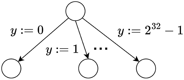
Figure 1. Handling variables in GPUEXPLORE 2.0.

Furthermore, in general, GPU state space exploration tools are not user-friendly. Providing input is tedious, requiring manually setting up low-level descriptions of models (Wijs et al., 2016b; DeFrancisco et al., 2020) or using a chain of other tools (Wijs et al., 2016b; Wei et al., 2019). For GPUEXPLORE 3.0, we wanted to change that and directly support a richer modeling language. The tool altogether avoids storing the input model in memory. To make this possible and high-performance, we developed a code generator that produces GPU code specific for exploring the state space of a given input model. Conceptually, this mechanism is similar to how SPIN transforms PROMELA models to pan code (Holzmann, 1997). GPUEXPLORE 3.0 is the first GPU tool to apply such a code generator. Furthermore, in this study, we propose how to perform memory-efficient complete state space exploration on a GPU for concurrent finite-state machines (FSMs) with data. To make this possible, we are the first to investigate the storage of binary trees in GPU hash tables to form a tree database, propose new algorithms to find and store trees in a fine-grained parallel fashion, experiment with a number of GPU-specific configurations, and propose two novel hashing techniques called compact-cuckoo hashing and compact multiple-functions hashing, which enable the use of Cleary compression (Cleary, 1984; Darragh et al., 1993) on GPUs. To achieve the desired result of the new algorithms, we have to tackle the following challenges: (1) CPU-based algorithms are recursive, but GPUs are not suitable for recursion, and (2) accessing GPU global memory, in which the hash tables reside, is slow. This research marks an important step to pioneer practical GPU accelerated model checking as it can be extended to checking functional properties of models with data and paves the way to investigate the use of binary decision diagrams (Lee, 1959) for symbolic model checking.

Contributions

The current article combines and extends the following contributions published previously by Wijs and Osama (2023a,b):

1. The overall workflow of GPUEXPLORE 3.0 is presented.

2. The new hashing schemes and technical details of Cleary compression are discussed.

3. The GPU tree database is explained.

4. Experimental results are presented and discussed, comparing GPUEXPLORE 3.0 with the CPU tools SPIN and LTSMIN, on the one hand, and the GPU tools GRAPPLE and GPUEXPLORE 2.0, on the other hand.

Compared to these two earlier articles, the following new contributions are introduced:

1. The new hashing schemes are presented in a separate section, putting more emphasis on the novelty of that contribution and explaining it in greater detail.

2. The technical details of the tree database are explained in much more detail. Two algorithms are presented for the first time, one for the fetching of state trees and one that links the other algorithms together.

3. A new method is proposed to employ multiple GPUs, all residing on the same machine, for complete state space exploration. In such a setting, peer-to-peer communication allows the threads of each GPU to directly access the memory of other GPUs, and this method is the first multi-GPU state space exploration procedure in the literature. To achieve multi-GPU state space exploration, we have to tackle a number of challenges: (1) a good load balancing algorithm needs to be obtained such that each GPU roughly has the same amount of exploration work and the number of states to store, and (2) since states are stored as binary trees, a mechanism must be designed that assigns every constructed binary tree in its entirety to a particular GPU.

4. The impact of scaling up the number of GPUs on which GPUEXPLORE runs on its performance is experimentally assessed, as well as the load balancing that the method achieves.

The structure of the article is as follows. In Section 2, we discuss related work on GPU hash tables. Section 3 presents background information on GPU programming, memory, and multi-GPU communications. In Section 4, our new hashing schemes are presented. Section 5 describes the input modeling language and how a model written in that language is used as input for GPUEXPLORE. Section 6 addresses the challenges when designing a GPU tree table and presents our new algorithms for handling state trees, both when using a single GPU and when using multiple GPUs on the same machine. Experimental results are given in Section 7. Finally, in Section 8, conclusion and our future work plans are discussed.

2 Related work

In the earliest research on GPU explicit state space exploration, GPUs performed part of the computation, specifically successor generation (Edelkamp and Sulewski, 2010a,b) and property checking, once the state space has been generated (Barnat et al., 2012). This was promising, but the data copying between main and GPU memory and the computations on the CPU was detrimental for performance. As mentioned in Section 1, the first tool that performed the entire exploration on a GPU was GPUEXPLORE (Wijs and Bošnački, 2014, 2016; Neele et al., 2016; Wijs, 2016; Wijs et al., 2016b). A similar exploration engine was later proposed by Wu et al. (2015). An approach that applied a GPU to explore the state space of PROMELA models, i.e., the models for the SPIN model checker (Holzmann, 1997), was presented by Bartocci et al. (2014). This approach was later adapted to the swarm checker GRAPPLE by DeFrancisco et al. (2020), which can efficiently explore very large state spaces, but at the cost of losing completeness. Finally, the model checker PARAMOC for pushdown systems was presented by Wei et al. (2018, 2019).

The above techniques demonstrate the potential for GPU acceleration of state space exploration and explicit-state model checking, being able to accelerate those procedures tens to hundreds of times, but they all have serious practical limitations. Several procedures limit the size of state vectors to 64 bits (Bartocci et al., 2014; Wu et al., 2015) or the size of transition encodings to 64 bits (Wei et al., 2018, 2019). GRAPPLE uses bitstate hashing, which rules out the ability to detect that all reachable states have been explored, which is crucial to prove the absence of undesired behavior. PARAMOC verifies push-down systems but does not support concurrency and abstracts away data. GPUEXPLORE 2.0 does not efficiently support models with variables (Wijs and Bošnački, 2014; Wijs et al., 2016b). When adding variables, the amount of memory needed grows rapidly due to the growing input model and inefficient state storage.

Since in explicit state space exploration, states are typically stored in a hash table (Cormen et al., 2009), we next discuss research on hash tables for the GPU. A GPU hash table is often implemented as an array, where the elements represent the hash table buckets. A recent survey of GPU hash tables by Lessley (2019) identifies that when using integer data items and unordered insertions and queries, cuckoo hashing (Pagh and Rodler, 2001) is (currently) the best option compared to techniques such as chaining (Ashkiani et al., 2018) or robin hood hashing (García et al., 2011), and the cuckoo hashing of Alcantara et al. (2012) is particularly effective. In cuckoo hashing, collisions, i.e., situations where a data item e is hashed to an already occupied bucket, are resolved by evicting the encountered item e′, storing e, and moving e′ to another bucket. A fixed number of m hash functions is used to have multiple storage options for each item. Item lookup and storage is therefore limited to m memory accesses but can lead to chains of evictions. Alcantara et al. (2012) demonstrated that, with four hash functions, a hash table needs ~1.25N buckets to store N items¹. Recent research by Awad et al. (2023) has demonstrated that using larger buckets, spanning multiple elements, that still fit in the GPU cache line is beneficial for performance and increases the average load factor, i.e., how much the hash table can be filled until an item cannot be inserted, to 99%.

Besides buckets, we also consider cuckoo hashing as used by Alcantara et al. (2012) and Awad et al. (2023); however, we are the first to investigate the storage of binary trees and the use of Cleary compression to store more data in less space. Libraries offering GPU hash tables, such as the one of Jünger et al. (2020), do not offer these capabilities. Furthermore, we are the first to investigate the impact of using larger buckets for binary tree storage embedded in a state space exploration engine.

The model checker GPUEXPLORE (Wijs and Bošnački, 2014; Wijs et al., 2016b; Cassee and Wijs, 2017) uses multiple hash functions to store a state. State evictions are never performed as each state is stored in a sequence of integers, making it impossible to store states atomically. This can lead to storing duplicate states, which tends to be worsened when states are evicted, making cuckoo hashing impractical (Wijs and Bošnački, 2016). Besides compact state storage, a second benefit of using trees with each tree node being stored in a single integer is that it allows arbitrarily large states to be stored atomically, i.e., a state is stored the moment the root of its tree is stored.

Because we store trees, with the individual nodes referencing each other, we do not consider alternative storage approaches, such as using a list that is repeatedly sorted, even though Alcantara et al. (2012) identified that using radix-sort (Merrill and Grimshaw, 2011) is competitive to hashing.

Although we are the first to propose a multi-GPU explicit state space exploration method, its design has been inspired by previous research on distributed model checking. In that setting, a cluster of machines is used to explore a state space, with the workers running on the different machines communicating with each other over a network. While communication is different from the single machine, multi-GPU setting, the approach to assign an owner, i.e., worker, to each state by using a hash function is used in both settings. Dill (1996) presented a distributed exploration algorithm for the MURϕ verifier. An approach for the distributed verification of stochastic models was proposed by Ciardo et al. (1998). Based on this approach, Behrmann et al. (2000) presented an algorithm for the timed model checker UPPAAL. A distributed state space exploration algorithm for the SPIN model checker was implemented by Lerda and Sista (1999). Garavel et al. (2001) presented a method to generate LTSs in a distributed way with the CADP toolbox. The DIVINE model checker was equipped with a distributed algorithm by Barnat et al. (2006). Finally, a collection of case studies in which the distributed state space exploration capabilities of the μCRL toolset were demonstrated were discussed by Blom et al. (2007).

3 GPU architecture

3.1 GPU programming

CUDA² is a programming interface that enables general purpose programming for a GPU. It has been developed and continually maintained by NVIDIA since 2007. In this study, we use CUDA with C++. Therefore, we use CUDA terminology when we refer to thread and memory hierarchies.

The left part of Figure 2 gives an overview of a GPU architecture. For now, ignore the bold-faced words and the pseudo-code. A GPU consists of a finite number of streaming multiprocessors (SM), each containing hundreds of cores. For instance, the Titan RTX and Tesla V100, which we used for this study, have 72 and 80 SMs together containing 4,608 and 5,120 cores, respectively. A programmer can implement functions named kernels to be executed by a predefined number of GPU threads. Parallelism is achieved by having these threads work on different parts of the data.

Figure 2

Figure 2. State space exploration on a GPU architecture.

When a kernel is launched, threads are grouped into blocks, usually of a size equal to a power of two, often 512 or 1,024. All the blocks together form a grid. Each block is executed by one SM, but an SM can interleave the execution of many blocks. When a block is executed, the threads inside are scheduled for execution in smaller groups of 32 threads called warps. A warp has a single program counter, i.e., the threads in a warp run in lock-step through the program. This concept is referred to as single instruction multiple threads (SIMT): each thread executes the same instructions but on different data. The threads in a warp may also follow diverging program paths, leading to a reduction in performance. For instance, if the threads of a warp encounter an if C then P1 else P2 construct, and for some, but not all, C holds, all threads will step through the instructions of both P1 and P2, but each thread only executes the relevant instructions.

GPU threads can use atomic instructions to manipulate data atomically, such as a compare-and-swap on 32- and 64-bit integers: ATOMICCAS(addr, compare, val) automically checks whether at address addr, the value compare is stored. If so, it is updated to val, otherwise no update is done. The actual value read at addr is returned.

Finally, the threads in a warp can communicate very rapidly with each other by means of intra-warp instructions. There are various instructions, such as SHUFFLE to distribute register data among the threads and BALLOT to distribute the results of evaluating a predicate. Since the availability of CUDA 9.0, threads can be partitioned into cooperative groups. If these groups have a size that completely divides the warp size, i.e., it is a power of two smaller than or equal to 32, then the threads in a group can use intra-warp instructions among themselves.

3.2 GPU memory

There are various types of memory on a GPU. The global memory is the largest of the various types of memory—24 GB in the case of the Titan RTX and 16 or 32 GB in the case of the Tesla V100, the two types of GPUs used for this study. The global memory can be used to copy data between the host (CPU-side) and the device (GPU-side). It can be accessed by all GPU threads and has a high bandwidth as well as a high latency. Having many threads executing a kernel helps to hide this latency; the cores can rapidly switch contexts to interleave the execution of multiple threads, and whenever a thread is waiting for the result of a memory access, the core uses that time to execute another thread. Another way to improve memory access times is by ensuring that the accesses of a warp are coalesced: if the threads in a warp try to fetch a consecutive block of memory in size not larger than the cache line size, then the time needed to access that block is the same as the time needed to access an individual memory address.

Other types of memory are shared memory and registers. Shared memory is fast on-chip memory with a low latency that can be used as block-local memory; the threads of a block can share data with each other via this memory. In GPUs such as the Titan RTX and the Tesla V100, each block can use up to 64 KB and 96 KB of shared memory, respectively. Register memory is the fastest and is used to store thread-local data. It is very small, though, and allocating too much memory for thread-local variables may result in data spilling over into global memory, which can dramatically limit the performance.

3.3 Peer-to-peer communication

In this study, we use a multi-GPU setup within a single node provided by the Amazon Web Services (AWS) computing cloud. Before the introduction of NVLink (NVIDIA Link) in 2014, GPU developers used to offload data transfer on the main PCI-express bus. However, the latter only offers very limited speed of up to 32 GB/s. With NVLink version 2.0, the Tesla V100 GPU can achieve peer-to-peer communication of up to 150 GB/s in one direction and 300 GB/s in both directions, which makes NVLink a viable option for accelerating state space exploration on multiple GPUs, as our experimental results in Section 7 demonstrate.

4 Compact-cuckoo and compact-multiple-functions hashing

As memory is a relatively scarce resource on a GPU, in explicit state space exploration, states should be stored in memory as compactly as possible, meaning that (1) the used hash table should be able to reach a high load factor, and (2) we are interested in techniques to store individual data elements, i.e., states, compactly.

Before we discuss GPUEXPLORE and the actual state space exploration in detail, in the current section, we focus on our first contribution, which addresses the hash table. It is important to note that states are stored in binary trees, thereby applying tree compression (Blom et al., 2008). An example of such a tree is given in Figure 3. In general, the leaves of the tree contain the actual state information, while the non-leaves contain references to their siblings. The state information is therefore stored in chunks that are equal in size to that of the tree nodes (in GPUEXPLORE, the node size is 64 bits, as nodes are stored in 64-bit integers). This means that, sometimes, system variables are cut in two. In the example of Figure 3, the value of the 32-bit integer variable x2 is split into one 20-bit entry and one 12-bit entry. More details about tree compression are presented in Section 6. The current section addresses several hashing techniques to store the trees in a hash table and our reasoning behind selecting some of them while disregarding others.

Figure 3

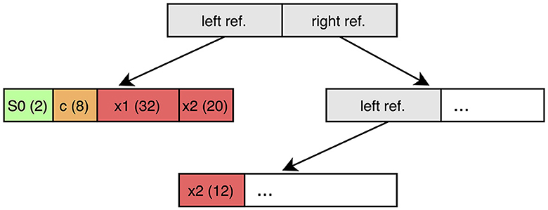
Figure 3. An example of a state represented by a binary tree.

In Section 2, we argued that cuckoo hashing is very effective on a GPU. Figure 4A demonstrates what happens with cuckoo hashing when collisions occur. When an element, in this case d, needs to be inserted, the first hash function h₀ is used to find a bucket. As this bucket is already occupied by another element, b, b is evicted and the hash function next in line for b is used to find a new bucket for b. In the figure, the hash functions that were used to store the elements are displayed in gray. In practice, one can identify the hash function previously used to store an element that is being evicted by applying each hash function on the element until the current address is obtained. In the example, b is then hashed to the bucket occupied by element a. Using function h₃, a is finally hashed to an empty bucket, thereby ending the eviction chain. Since eviction chains can be infinite in length, due to cyclic evictions, in practice, one has to set an upper bound on their length.

Figure 4

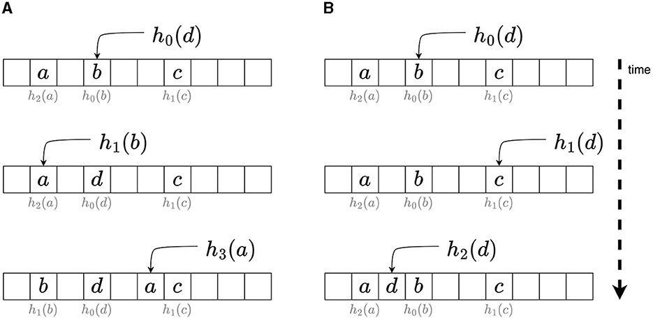
Figure 4. Collision handling with cuckoo hashing (A) and using multiple hash functions (B).

As cuckoo hashing frequently moves elements, it is not suitable for a hash table that stores binary trees. In such a table, the stored non-leaves contain references to their direct siblings. If those siblings were to be moved, the references used by their parents would become incorrect, and updating those would be too time-consuming.

However, one can instead use two hash tables, one for tree roots, the root table, and one for the other nodes, the internal table, as done by Laarman (2019). The roots are then not referred to by other nodes, and hence, cuckoo hashing can be applied on the root table.

In fact, when using two hash tables, we can be even more memory efficient. Laarman (2019) has shown that Cleary tables (Cleary, 1984; Darragh et al., 1993) can be very effective for storing state spaces. In Cleary hashing, each data element of K bits is split, possibly after its bits have been scrambled, into an address A and a remainder R. The remainder R is subsequently stored at address A in the hash table. To retrieve the original data element from the table, A and R need to be combined again. Note that any applied bit scrambling must be invertible to retrieve the original K bits. In other words, Cleary hashing achieves its compression by using the address where an element must be stored to encode part of the element itself.

To handle collisions in Cleary tables, order-preserving bidirectional linear probing (Amble and Knuth, 1974) is used, which involves scanning the table in two directions to find an empty bucket for a given element, starting at the one to which the element was hashed. The stored remainders are moved to preserve their order. An elaborate scheme is used that, for each stored remainder, allows finding the address at which it was supposed to be stored, even if it is not physically located there. It is crucial that this address can be retrieved, otherwise decompression would not be possible.

The frequent moving of remainders makes Cleary hashing, such as cuckoo hashing, unsuitable for storing entire trees, but as with cuckoo hashing, it can be used to store the roots of the trees. In this setting, for roots of size 2k, with k being the number of bits needed for a node reference, each root r is hashed (bit scrambled) with a hash function h to a 2k bit sequence, from which w < 2k bits are taken to be used as an index of a root table with exactly 2^w buckets, and at this position, the remaining 2k−w bits (the remainder) are stored. To enable decompression, h must be invertible; given a remainder and an address, h⁻¹ can be applied to obtain r.

In a multi-threaded CPU context, this approach scales well (Laarman, 2019), but the parallel approach by van der Vegt and Laarman (2011) and Laarman (2019) divides a Cleary table into regions, and sometimes, a region must be locked by a thread to safely reorder remainders. Unfortunately, the use of any form of locking, including fine-grained locking implemented with atomic operations, is detrimental for GPU performance. Furthermore, the absence of coherent caches in GPUs means that expensive global memory accesses may be needed when a thread repeatedly checks the status of an acquired lock.

As an elegant alternative, we propose two hashing schemes compact-cuckoo hashing and compact-multiple-functions hashing that combine Cleary compression with cuckoo hashing and with using a sequence of hash functions, respectively.

Multiple-functions hashing uses multiple hash functions, such as cuckoo hashing, but does not perform evictions. Figure 4 shows how multiple-functions hashing works. When a data element d is to be stored, first, hash function h₀ is used. If a collision occurs with an element b, the next hash function h₁ is used to find an alternative bucket for d. Storage fails if all possible buckets for d are full. This form of hashing resembles multiple-choice hashing (Azar et al., 1999), but there is an important difference: in multiple-choice hashing, all possible locations for an element are inspected, and one option is chosen. In cases where each bucket can store multiple elements, this choice is typically made with the goal of balancing the load in the buckets. In multiple-functions hashing, the first available option is selected. The reason that we consider multiple-functions hashing as opposed to multiple-choice hashing is due to the requirements that hashing should be performed massively in parallel and that, in state space exploration, states should never be stored multiple times, i.e., there should not be any redundancy in the hash table. Allowing choice in selecting a storage location for an element potentially leads to multiple threads simultaneously selecting different locations for the same element. The fact that, in state space exploration, a state (and the nodes in the tree representing it) tends to be encountered and therefore searched in the hash table, not once, but many times during exploration, makes redundant storage when allowing choice very likely.

Both cuckoo hashing and multiple-functions hashing can be combined with the compression approach of Cleary hashing in an elegant way, leading to hashing schemes with collision resolution mechanisms that are both simpler and more amenable to massive parallel hashing than the mechanism used in Cleary hashing. For both new schemes, we use m hash functions that are invertible and capable of scrambling the bits of a root to a 2k bit sequence (as in Cleary hashing). When we apply a function h_i (0 ≤ i<m) on a root r, we get a 2k bit sequence, of which we use w bits for an address d and store at d the remainder r′ consisting of 2k−w bits, together with ⌈log₂(m)⌉+1 bookkeeping bits. The ⌈log₂(m)⌉ bits are needed to store the ID of the used hash function (i), and the final bit is needed to indicate that the root is new (unexplored). It is possible to retrieve r by applying $h_i^{-1}$ on d and r′. In compact-cuckoo hashing, when a collision occurs, the encountered root is evicted, decompressed, and stored again using the hash function next in line for that root. In compact-multiple-functions hashing, instead of evicting the encountered root, an attempt is made to store a remainder of the new root with the hash function next in line. We refer to the application of Cleary compression to roots, either using compact-cuckoo hashing or compact-multiple-functions hashing, as root compression.

For the construction of invertible bit-scrambling functions, a number of possible arithmetic operations can be applied. For instance, a right xorshift, i.e., bitwise xor (^∧) combined with a bitwise right shift (≫), is invertible. Consider the operation

$y=x^(x\gg a),$

with a a constant smaller than the number of bits of x. The following sequence of operations retrieves the value of x from y:

$\begin{array}{l}x=y^(y\gg 2^0·a),\hfill \\ x=x^(x\gg 2^1·a),\hfill \\ x=x^(x\gg 2^2·a),\hfill \\ ⋮\hfill \end{array}$

The sequence continues until 2ⁱ·a exceeds the number of bits of x.

A second type of invertible operation that we applied in our functions is multiplication with a (large) odd number z, which can be inverted by multiplying with the modular multiplicative inverse z⁻¹ of z, i.e., z·z⁻¹ mod m = 1 if we are working with numbers in the range [0, m〉. An approach based on Newton's method can be used to find modular multiplicative inverses (Dumas, 2014).

In Section 2, we mentioned the use of buckets in a GPU hash table that can contain multiple elements. When a hash table is divided into buckets, each bucket having space for 1 < n ≤ 32 elements that still fit in the GPU cache line, then cooperative groups of n threads each can be created, and the threads in a group can work together for the fetching and updating of buckets. When an element is hashed to a bucket, the group fetches the n consecutive positions of that bucket and collectively inspects those positions for the presence of that element. In case the element is to be stored, an empty position is collectively identified, and the element is stored by one thread of the group at that position. If the bucket is full, another bucket must be selected according to the hashing scheme. The use of larger buckets results in more coalesced memory accesses and reduces thread divergence. However, it also means that fewer tasks can be performed in parallel.

In Section 6.5, an algorithm is discussed in which a cooperative group of threads performs a find-or-put operation for a given tree node. In such an operation, it is checked whether the node is already stored in the hash table, and if it is not, it is then inserted into the table.

5 From an SLCO model to GPUexplore code

5.1 The simple language of communicating objects

Figure 5 presents the workflow of GPUEXPLORE 3.0. It accepts models written in the Simple Language of Communicating Objects (SLCO) (de Putter et al., 2018). An SLCO model consists of a finite number of finite state machines (FSMs) that concurrently execute transitions. The FSMs can communicate via globally shared variables, and each FSM can have its own local variables. Variables can be of type Bool, Byte, and (32-bit) Integer, and there is support for arrays of these types. We use (system) states s, s′, … to refer to entire states of the system, and FSM states σ, σ′, … to refer to the states of an individual FSM. A system state is essentially a vector containing all the information that together defines a state of the system, i.e., the current states of the FMSs and the values of the variables.

Figure 5

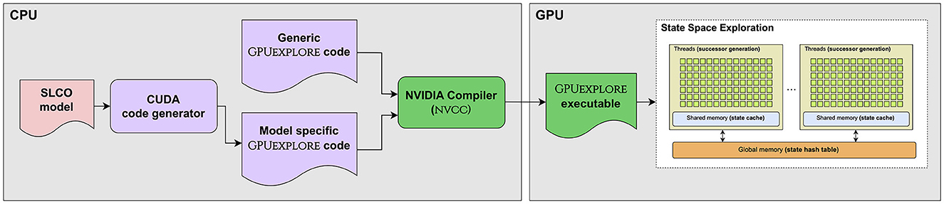
Figure 5. The workflow of GPUEXPLORE 3.0.

Each FSM in an SLCO model has a finite number of states and transitions. An FSM transition $tr=\sigma \stackrel{st}{\to }{\sigma }^{\prime }$ indicates that the FSM can change state from σ to σ′ if and only if the associated statement st is enabled. A statement is either an assignment, an expression, or a composite. Each can refer to the variables in the scope of the FSM. An assignment is always enabled and assigns a value to a variable; an expression is a predicate that acts as a guard: it is enabled if and only if the expression evaluates to true. Finally, a composite is a finite sequence of statements st₀; …;st_n, with st₀ being either an expression or an assignment and st₁, …, st_n being assignments. A composite is enabled if and only if its first statement is enabled. A transition $tr=\sigma \stackrel{st}{\to }{\sigma }^{\prime }$ can be fired if st is enabled, which results in the FSM atomically moving from state σ to state σ′, and any assignments of st being executed in the specified order. When tr is fired while the system is in a state s, then after firing, the system is in state s′, which is equal to s, apart from the fact that σ has been replaced by σ′, and the effect of st has been taken into account. We call s′ a successor of s.

The formal semantics of SLCO defines that each transition is executed atomically, i.e., it cannot be interrupted by the execution of other transitions. The FSMs execute concurrently using an interleaving semantics. Finally, the FSMs may have non-deterministic behavior, i.e., at any point of execution, an FSM may have several enabled transitions.

On the left-hand side of Figure 6, an example SLCO FSM is shown. The FSM is taken from a translation of the adding.1 model from the BEEM benchmark suite (Pelánek, 2007). It has three process states, with Q being the initial state. The transition statements refer to two of the three variables in the model, c and x1.

Figure 6

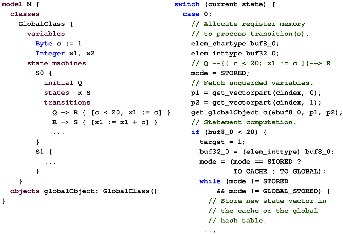
Figure 6. The SLCO model M and its generated code are shown on the left and the right, respectively.

5.2 From SLCO to GPUexplore

Given an input model, a code generator, implemented in PYTHON using TEXTX (Dejanović et al., 2017) and JINJA2³, produces model-specific code written in NVIDIA's CUDA C++ (see Figure 5). This code entails next-state computation functions, i.e., functions that, given a system state s, produce the successor system states that can be reached from s by executing a transition. In the model-specific code, one next-state computation function is produced for each FSM in the model, allowing for the successor states of a single state to be constructed in parallel, with the functions executed by different threads.

Given a system state and an FSM, a GPU thread generates successors by executing the corresponding next-state computation function. This function contains a big switch statement to consider the execution of transitions based on the current state of the FSM. On the right-hand side of Figure 6, part of the generated next-state computation function is shown for the FSM on the left. In this example, if the current state of this FSM, fetched from the system state and stored in the variable current_state, is Q (encoded as 0), then the thread will retrieve the value of c and store it in the variable buf8_0, located in thread-local register memory. If this value is smaller than 20, the target FSM state is set to 1 (R), and the register variable buf32_0, associated with x1, is assigned the value of buf8_0, i.e., c. Next, the thread will construct the new successor state by combining the original state with the new values and store the new state.

This parallel construction of successors does not influence the correctness of the exploration: together, the threads end up exploring all possible execution paths of the input SLCO model. System states are stored as binary trees. The model-specific code involves the handling of those trees, the structure and size of which depend on the input model.

Combined with GPUEXPLORE's generic code, which implements the control flow and the hash tables and their methods, the code is compiled using NVIDIA's NVCC compiler. The resulting executable is suitable for CUDA-compatible GPUs with at least compute capability 7.0. Figure 2 presents how the different components of the state space exploration engine map onto a GPU. In the global memory, a large hash table (we call it $\mathcal{G}$) is maintained to store the states visited until then. At the start, the initial state of the input model is stored in $\mathcal{G}$. Each state in $\mathcal{G}$ has a Boolean flag new, indicating whether the state has already been explored, i.e., whether or not its successors have been constructed.

On the right-hand side of Figure 2, the state space exploration algorithm is explained from the perspective of a thread block. While the block can find unexplored states in $\mathcal{G}$, it selects some of those for exploration. In fact, every block has a work tile residing in its shared memory, of a fixed size, which the block tries to fill with unexplored states at the start of each exploration iteration. Such an iteration is initiated on the host side by launching the exploration kernel. States are marked as explored, i.e., not new, when added by threads to their tile. Next, every block processes its tile. For this, each thread in the block is assigned to a particular state/FSM combination. Each thread accesses its designated state in the tile and analyses the possibilities for its designated FSM to change state, as explained earlier.

The generated successors are stored in a block-local state cache, which is a hash table in the shared memory. This avoids repeated accessing of global memory, and local duplicate detection filters out any duplicate successors generated at the block level. Once the tile has been processed, the threads in the block together scan the cache once more and store the new states in $\mathcal{G}$ if they are not already present. When states require no more than 32 or 64 bits in total, including the new flag, they can simply be stored atomically in $\mathcal{G}$ using compare-and-swap. However, sufficiently large systems have states consisting of more than 64 bits. In this study, we therefore focus on working with these larger states and consider storing them as binary trees. In Section 6, we present new algorithms to efficiently process and store state binary trees on GPUs.

6 GPU state space exploration with a tree database

6.1 CPU tree storage

The number of data variables in a model and their types can have a drastic effect on the size of the states of that model. For instance, each 32-bit integer variable in a model requires 32 bits in each state. As the amount of global memory on a GPU is limited, we need to consider techniques to store states in a memory-efficient way. One technique that has proven itself for CPU-based model checkers is tree compression (Blom et al., 2008), in which system states are stored as binary trees. A single hash table can be used to store all tree nodes (Laarman et al., 2011). Compression is achieved by having the trees share common subtrees. Its success relies on the observation that states and their successors tend to be different in only a few data elements. In Laarman et al. (2011), it is experimentally assessed that tree compression compresses better than any other compression technique identified by the authors for explicit state space exploration. They observe that the technique works well for a multi-threaded exploration engine. Moreover, they propose an incremental variant that has a considerably improved runtime performance as it reduces the number of required memory accesses to a number logarithmic in the length of the state vector.

Figure 7 shows an example of applying tree compression to store four state vectors. The black circles should be ignored currently. Each letter represents a part of the state vector that is k bits in length. We assume that, in k bits, a pointer to a node can also be stored and that each node therefore consists of 2k bits. The vector <A,B,C,D,E> is stored by having a root node with a left leaf sibling <A,B> and the right sibling being a non-leaf that has both a left leaf sibling <C,D> and the element E. In total, storing this tree requires 8k bits. To store the vector <A′,B,C′,D,E>, we cannot reuse any of these nodes, as <A′,B> and <C′,D> have not been stored yet. This means that all pointers have to be updated as well and, therefore, a new root and a new non-leaf containing E are needed. Again, 8k bits are needed. For <A,B′,C,D,E′>, we have to store a new node <A,B′>, a new root, and a new non-leaf storing E′, but the latter can point to the already existing node <C,D>. Hence, only 6k bits are needed to store this vector. Finally, for <A′,B,C,D,E′>, we only need to store a new root node, as all other nodes already exist, resulting in only needing 2k bits. It has been demonstrated that, as more and more state vectors are stored, eventually new vectors tend to require 2k bits each (Laarman et al., 2011; Laarman, 2019).

Figure 7

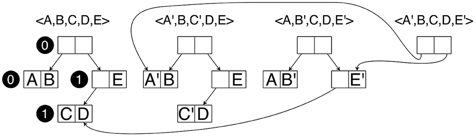
Figure 7. An example of storing state vectors as binary trees.

To emphasize that GPU tree compression has to be implemented vastly differently from the typical CPU approach, we first explain the latter and the incremental approach (Laarman et al., 2011). Checking for the presence of a tree and storing it, if not yet present, is typically done by means of recursion (outlined by Algorithm 1). For now, ignore the red underlined text. The STORE function returns the address of the given node in $\mathcal{G}$, if present; otherwise, it stores the node and returns its address, and the FINDORPUT-CPU function first recursively checks whether the siblings of the node are stored, and if not, stores them, after which the node itself is stored. A node has pointers left and right to addresses of $\mathcal{G}$, and there are functions to check for the existence of and retrieve the siblings of a node.

Algorithm 1

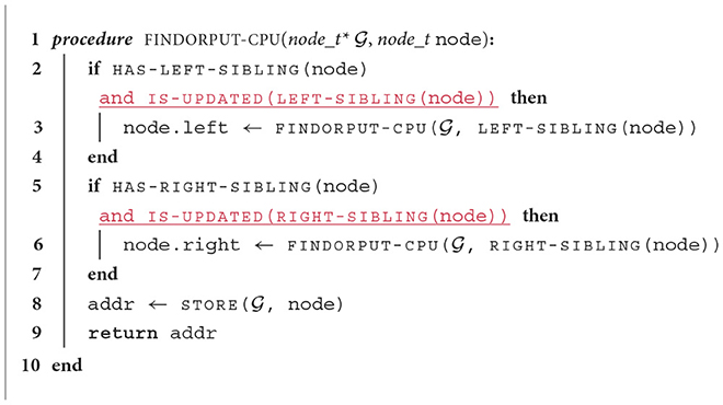
Algorithm 1. Tree-based find-or-put, CPU version.

In the incremental approach, when creating a successor s′ of a state s, the tree for s, say T(s), is used as the basis for the tree T(s′). When T(s′) is created, each node inside it is first initialized to the corresponding node in T(s), and the leaves are updated for the new tree. This “updated” status propagates up: when a non-leaf has an updated sibling, its corresponding $\mathcal{G}$ pointer must be updated when T(s′) is stored in $\mathcal{G}$, but for any non-updated sibling, the non-leaf can keep its $\mathcal{G}$ pointer. When incorporating the red underlined text in Algorithm 1, the incremental version of the function is obtained. With this version, tree storage often results in fewer calls to STORE, i.e., fewer memory accesses.

There are two main challenges when considering GPU incremental tree storage: (1) recursion is detrimental to performance, as call stacks are stored in global memory (and with thousands of threads, a lot of memory would be needed for call stacks), and (2) the nodes of a tree tend to be spread all over the hash table, potentially leading to many random accesses. To address these challenges, we propose a procedure in which threads in a block store sets of trees together in parallel.

6.2 GPU tree generation

When states are represented by trees, the tile of each thread block cannot store entire states, but it can store $\mathcal{G}$ indices of roots of trees. To speed up successor generation and avoid repeated uncoalesced global memory accessing, the trees of those roots are retrieved and stored in the shared memory (state cache) by the thread block. Once this has been done, successor generation can commence. Section 6.3 describes how state trees are retrieved from global memory. First, we explain how new trees are generated.

Figure 8 shows an example of the state cache evolving over time as a thread generates the successor s′ = <A,B′,C,D,E′> of s = <A,B,C,D,E>, with the trees as shown in Figure 7. Each square represents a k-bit cache entry. In addition to the two entries needed to store a node, we also use one (gray) entry to store two cache pointers or indices and assume that k bits suffice to store two pointers (in practice, we use k = 32, which is enough, given the small size of the state cache). Hence, every pair of white squares followed by a gray square constitutes one cache slot. Initially (shown at the top of Figure 8), the tile has a cache pointer to the root of s, of which we know that it contains the $\mathcal{G}$ addresses a₀ and a₁ to refer to its siblings. In turn, this root points, via its cache pointers, to the locally stored copies of its siblings. The non-leaf one contains the global address a₂. A leaf has no cache pointers, denoted by “–.” When creating s′, first, the designated thread constructs the leaf <A,B′>, by executing the appropriate generated CUDA function (see Section 5.1), and stores it in the cache. In Figure 8, this new leaf is colored black to indicate that it is marked as new. Next, the thread creates a copy of < a₂,E>, together with its cache pointers, and updates it to < a₂,E′>. Finally, it creates a new root, with cache pointers pointing to the newly inserted nodes. This root still has global address gaps to be filled in (the “?” marks), since it is still unknown where the new nodes will be stored in $\mathcal{G}$.

Figure 8

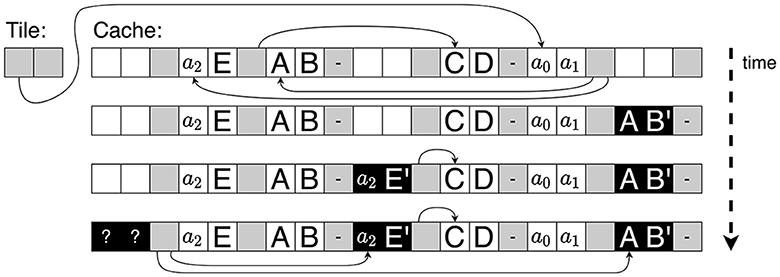
Figure 8. Successor generation: deriving <A,B′,C,D,E′> from <A,B,C,D,E>.

The reason that we store global addresses in the cache is not to access the nodes they point to but to achieve incremental tree storage: in the example, as the global address a₂ is stored in the cache, there is no need to find <C,D> in $\mathcal{G}$ when the new tree is stored; instead, we can directly construct < a₂,E′>. This contributes to limiting the number of required global memory accesses.

Note that there is no recursion. Given a model, the code generator determines the structure of all state trees, and based on this, the code to fetch all the nodes of a tree and to construct new trees is generated. As we do not consider the dynamic creation and destruction of FSMs, all states have the same tree structure.

6.3 GPU tree fetching

Before successors can be generated, the trees of the roots referred to in the tile must be fetched from $\mathcal{G}$. Algorithm 2 presents how this can be done in a cooperative group synchronous way to maximize parallelism. This particular code has been generated for trees with a structure as in Figure 7. The FETCH function is executed by cooperative groups of size n = 2ⁱ for i∈[0, 5]. This size is predetermined to be the smallest value that is still at least as large as the number of leaves in a tree; hence, n = 2 in the example. The function is set up in such a way that each thread eventually stores one leaf in its leaf variable and possibly one non-leaf node in its node variable. In general, the leaves of a tree are numbered from left to right starting with 0, and the non-leaves are numbered from the root downwards and left to right starting with 0. In Figure 7, the black circles define the numbering for the nodes, which is used to assign threads.

Algorithm 2

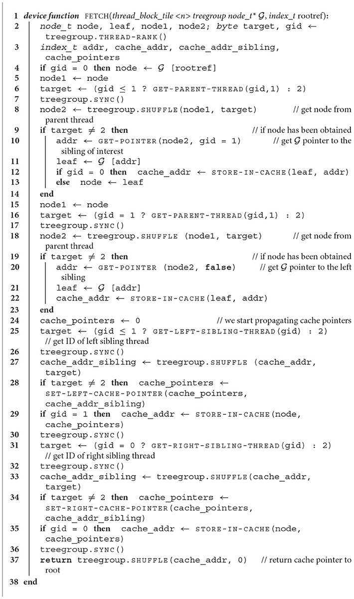
Algorithm 2. Cooperative group synchronous fetching of state trees.

Besides the cooperative group, a pointer to $\mathcal{G}$ is given, as well as the $\mathcal{G}$ index of a tree root (rootref). At line 2 (l.2), local node variables (64-bit integers) are declared, and two byte variables, the second of which (gid) is set to the index of the thread in its group, between 0 and n−1. At l.3, variables to store indices are declared; depending on the size of $\mathcal{G}$, these are either 32- or 64-bit integers.

At l.4, the group leader (with gid = 0) reads the designated root from $\mathcal{G}$ and stores it in the local variable node. This content is copied into node1 for communication with the other threads at l.5. At l.6, each thread t retrieves the ID of its thread parent t′ with respect to the node t has to retrieve at tree level 1. The function GET-PARENT-THREAD provides this ID, which in the example is 0 for both threads in the group, as the root is stored by thread 0. For any other thread, if fetch would be called with n>2, the ID is set to the default 2, which is larger than the number of threads needed. After synchronization (l.7), a shuffle instruction (SHUFFLE) is performed, by which each thread obtains the value of the node1 variable of its parent thread, and stores it in node2. If target = 2, nothing is actually retrieved, and l.10–13 are not executed. Otherwise, the $\mathcal{G}$ address of the left or right sibling of node2 is retrieved at l.10; if the given predicate gid = 1 is false, the left pointer is retrieved, otherwise the right pointer is retrieved.

The sibling node is fetched and stored in leaf at l.11 and stored in the cache at l.12 if gid = 0, i.e., if the node is actually a leaf. Otherwise, the node is stored in node (l.13). At l.18–23, this procedure is repeated once more, this time only for thread 1, which still needs to retrieve the left sibling of its non-leaf (see Figure 7). After this, all nodes have been fetched, and the non-leaves can be stored in the cache, which requires collecting the necessary cache indices to point from each non-leaf to its siblings. These indices are stored in a 32-bit integer cache_pointers. At l.25–27, the threads obtain the cache index of the left sibling of their node stored in node, using the function GET-LEFT-SIBLING-THREAD to obtain the ID of the thread storing the left sibling. At l.28, this index is stored in cache_pointers. At that moment, the non-leaf of thread 1 can be stored in the cache (l.29). At l.31–34, the index of the right sibling of the root is obtained and stored in cache_pointers of thread 0. At l.35, the root is stored. Finally, the cache index of this root is sent to the other thread in the group and returned by all threads (l.37).

The cooperative group synchronous approach uses multiple threads to fetch a single tree. As nodes are essentially distributed randomly over $\mathcal{G}$, using many threads helps to hide the latency of fetching. In addition, the use of the combined register memory of the group allows handling larger trees efficiently.

6.4 GPU tree storage at block level

Once a block has finished generating the successors of the states referred to by its tile, the state cache contents must be synchronized with $\mathcal{G}$. Algorithm 3 presents how this is done. The FINDORPUT-MANY function is executed by all threads in the block simultaneously. It consists of an outer while-loop (l.5–36) that is executed as long as there is work to be done. The code uses a cooperative group called bg, which is created to coincide with the size of a hash table bucket (bucketsize). Bucket sizes are typically a power of two, and not larger than 32. When buckets have size one, these groups consist of only a single thread each. At l.4, the offset of each thread is determined, i.e., its ID inside its group, ranging from 0 to the size of the group.

Algorithm 3

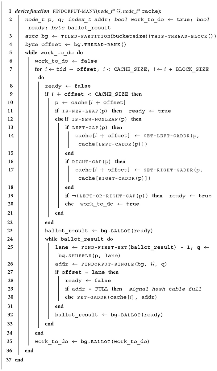
Algorithm 3. Tree-based find-or-put-many at the thread block level.

Every thread that still has work to do (l.5) enters the for-loop of l.7–34, in which the contents of the state cache is scanned. The parallel scanning works as follows: every thread first considers the node at position tid−offset of the cache, with tid being the thread's block-local ID. This node is assigned to the thread with bg ID 0. If that index is still within the cache limits, all threads of bg have to move along, regardless of whether they have a node to check or not. At the next iteration of the for-loop, the thread jumps over BLOCK_SIZE nodes as long as the index is within the cache limits.

The main goal of this loop is to check which nodes are ready for synchronization with $\mathcal{G}$. Initially, this is the case for all nodes without global address gaps (see Section 6.2). Each thread first checks whether its own index is still within the cache limits (l.9). If so, the node p is retrieved from the cache at l.10. If it is a new leaf, ready is set to true to indicate that the active thread is ready for storage (l.11). If the node is a new non-leaf (l.12), it is checked whether the node still has global address gaps. If it has a gap for the left sibling (l.13), this left sibling is inspected via the cache pointer to this sibling [retrieved with the function LEFT-CADDR (l.14)]. The function SET-LEFT-GADDR checks whether the cache pointers of that sibling have been replaced by a global memory address and, if so, uses that address to fill the gap. The same is done for the right sibling at l.16–18. If, after these operations, the node p contains no gaps (l.19), ready is set to true. If the node still contains a gap, another loop iteration is required, hence work_to_do is set to true (l.20).

At l.23, the threads in the group perform a ballot, resulting in a bit sequence indicating for which threads ready is true. As long as this is the case for at least one thread, the while-loop at l.24–33 is executed. The function FIND-FIRST-SET identifies the least significant bit set to 1 in ballot_result (l.25), and the SHUFFLE instruction results in all threads in bg retrieving the node of the corresponding bg thread. This node is subsequently stored by bg, by calling FINDORPUT-SINGLE (l.26; explained in Section 6.5). Finally, the thread owning the node (l.27) resets its ready flag (l.28), and if the hash table is considered full, then it reports this globally (l.29). Otherwise, it records the global address of the stored node (l.30). After that, ballot_result is updated (l.32). Once the for-loop is exited, the bg threads determine whether they still have more work to do (l.35).

6.5 Single node storage at bucket group level

In this section, we address how individual nodes are stored by a cooperative group bg. GPUEXPLORE allows configuration of its hash tables in the following ways (see Section 4): the default hashing scheme is multiple-functions hashing. Root compression can be turned on or off. If it is turned on, instead of one single hash table, a root table and an internal table is used. When root compression is used, cuckoo hashing can be turned on. Finally, buckets can be used of size 1 and of size 8 (for the root table) and 16 (for the internal table and when root compression is off). These different configuration options are experimentally compared in Section 7.1.

Algorithm 4 presents one version of the FINDORPUT-SINGLE function to which a call in (Algorithm 3) is redirected when a root is provided and cuckoo hashing is applied. Here, $\mathcal{G}$ is a root table, as explained in Section 4. In FINDORPUT-SINGLE, a second function FOP-CUCKOO-ROOT (l.9–28) is called repeatedly as long as nodes are evicted or until the pre-configured MAX_EVICT has been reached, which prevents infinite eviction sequences (l.4). The function FOP-CUCKOO-ROOT returns the address where the given node was found or stored, and the node is either the node that had to be inserted or the one that was already present.

Algorithm 4

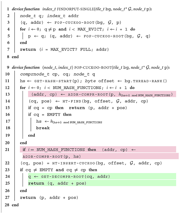
Algorithm 4. Single node find-or-put, at bucket group level.

In the FOP-CUCKOO-ROOT function, lines highlighted in purple are specific for root compression, i.e., Cleary compression applied to roots (see Section 4), while the green highlighted lines concern cuckoo hashing, thereby addressing node eviction. The ID of the first hash function to be used for node p, encoded in p itself, is stored in hs (l.11), and each thread determines its bg offset. Next, the thread iterates over the hash functions, starting with function hs (l.12–20). The $\mathcal{G}$ address and node remainder cp are computed at l.13. If the node is new, the remainder is marked as new. If root compression is not used, we have p = cp. Then, the function HT-FIND is called to check for the presence of the remainder in the bucket starting at addr (l.14). If HT-FIND returns the remainder, then it was already present (l.15), and this can be returned. Note that the returned address is (addr + pos), i.e., the offset at which the remainder can be found inside the bucket is added to addr. Alternatively, if EMPTY is returned, the node is not present and the bucket is not yet full. In this case, a bucket has been found where the node can be stored. The used hash function is stored in hs (l.17) and the for-loop is exited (l.18).

At l.21, if a suitable bucket for insertion has not been found, the initial hash function hs is selected again. At l.22, the function HT-INSERT-CUCKOO is called to insert cp. This function is presented in Algorithm 5. Finally, if a value other than the original remainder cp or EMPTY is returned, another (remainder of a) node has been evicted, which is decompressed and returned at l.24–25. Otherwise, p is returned with its address (l.27).

Algorithm 5

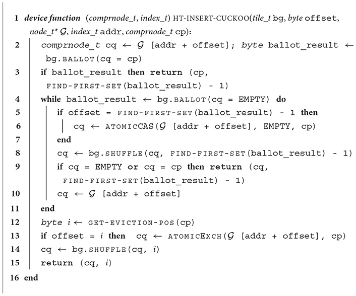
Algorithm 5. Single node insertion, at bucket group level.

A version of FINDORPUT-SINGLE in which multiple-functions hashing is used instead of cuckoo hashing is very similar to Algorithm 4. Essentially, it can be obtained by having FOP-CUCKOO-ROOT return that the bucket is full at l.24–25 instead of executing the green highlighted lines.

Finally, we present HT-INSERT-CUCKOO in Algorithm 5. The function HT-FIND is not presented, but it is almost equal to l.2–3 of Algorithm 5. At l.2, each thread in bg reads its part of the bucket $\mathcal{G}$[addr + offset], and checks if it contains cp, the remainder of p. If it is found anywhere in the bucket, the remainder with its position is returned (l.3). In the while-loop at l.4–11, it attempts to insert cp in an empty position. In every iteration, an empty position is selected (l.5) and the corresponding thread tries to atomically insert cp (l.6). At l.8, the outcome is shared among the threads. If it is either EMPTY or the remainder itself, it can be returned (l.9). Otherwise, the bucket is read again (l.10). If insertion does not succeed, l.12 is reached, where a hash function is used by GET-EVICTION-POS to hash cp to a bucket position. The corresponding thread exchanges cp with the node stored at that position (l.13). After the evicted node has been shared with the other threads (l.14), it is returned together with its position (l.15).

6.6 Putting it all together

In this section, we assemble the new algorithms we presented in the previous sections and show how they fit together in the state space exploration procedure. Algorithm 6 outlines the steps that are executed from the initialization of resources until the end of exploration, after which the number of reachable states is reported. It is assumed that root compression is applied, meaning that both a root table and an internal table are used.

Algorithm 6

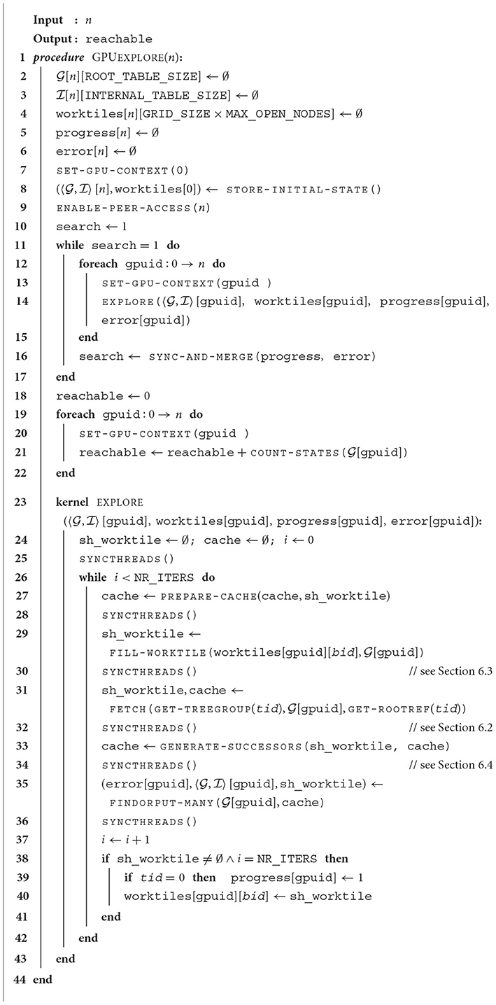
Algorithm 6. GPUexplore main exploration procedure.

The algorithm takes as input n number of GPUs and allocates n root tables of size ROOT_TABLE_SIZE (l.2). The use of more than one GPU is discussed in Section 6.7. At the moment, assume that n = 1. The ROOT_TABLE_SIZE is always a power of 2 and must be chosen in such a way that all required data structures fit in the global memory. For example, if a GPU has 16 GB of memory, then a root table consisting of 2³¹ 32-bit integers (or 8 GB in total) can be allocated. In addition, the internal table must be allocatable in addition to the worktiles array and the progress and error variables (l.3–6). The internal table is configured to have a fixed INTERNAL_TABLE_SIZE for 2²⁹ 64-bit integers (or 4 GB in total). The worktiles array has a predefined size of the number of thread blocks (GRID_SIZE) times the maximum work tile size (MAX_OPEN_NODES). Its purpose is to store the current contents of a work tile at the end of an exploration round, which consists of an execution of the EXPLORE kernel (l.38) and fetching the current work tile at the beginning of a round (l.27). This array resides in global memory and is needed since shared memory is wiped automatically once a kernel has terminated. The progress and error variables are used to keep track of whether a next exploration round is needed and whether an error has occurred in the current round, respectively.

At l.7, the current GPU context is set to GPU 0. Doing this will instruct the compiler to run the next GPU operations and memory allocations on the designated GPU. The initial state is stored by the routine STORE-INITIAL-STATE. When this is done, the tree of the initial state is stored in the hash tables, and a reference to the root of this tree has been added to the work tile of the thread block that stored the initial state. In general, when a thread block stores a new state in the hash tables, it immediately adds a reference to the root of that state to its own work tile, unless that tile is already completely filled with references. This process is called work claiming and prevents the block from having to scan the global memory for new exploration work at the start of every exploration round. This scanning is time-consuming as it involves many global memory accesses. At l.9, we enable bi-directional peer access for the n GPUs to allow all threads to access data freely of every GPU during the kernel execution. This can be ignored at the moment but is relevant in Section 6.7.

At l.10–17, the actual exploration of the state space is performed. The search flag at l.10 is used to ensure that the search continues as long as there are pending states to explore on the GPU. This is done iteratively inside the while loop at l.11–17. The while loop is executed on the host, and inside it, the GPU kernel EXPLORE is called repeatedly, i.e., exploration rounds are launched. Since for now, we consider the use of a single GPU, the loop at l.12–15 involves one iteration only. Inside it, the EXPLORE kernel is launched [SET-GPU-CONTEXT(gpuid ) at l.13 selects the appropriate GPU]. The EXPLORE kernel is given at l.23–43. Once an exploration round has finished, the GPU is synchronized with the host using the SYNC-AND-MERGE function at l.16. This function checks if another exploration round is needed and whether an error has occurred (for instance, because the hash tables are considered full and node storage has failed). In general, for n GPUs, the search flag is updated as follows:

$\begin{array}{l}(\mathbf{\forall } i.(0\le i<n).\mathtt{\text{error}}[i]=0)\\ \wedge (\mathbf{\exists } j.(0\le j<n).\mathtt{\text{progress}}[j]=1)\iff \mathtt{\text{search}}=1.\end{array}$

For a single GPU, this means that search is set to 1 if and only if error = 0 and progress = 1. Once the exploration has terminated, the number of reachable states, which coincides with the number of roots stored in $\mathcal{G}$, is counted at l.18–22.

At l.23–43, the EXPLORE kernel is described. First of all, at l.24, (block-local) shared-memory arrays for the work tile and state cache are created and initialized. In addition, a variable i is set to 0. This variable is used to keep track of the number of iterations performed inside a single EXPLORE kernel execution. The total number of iterations per kernel execution can be predefined by setting the NR_ITERS constant (l.26). The benefit of performing more than one iteration per kernel execution is that the cache contents after one iteration can be reused by the next. In particular, this means that any states claimed for exploration in one iteration do not need to be fetched from the global hash tables at the start of the next iteration, since they already reside in the cache.

At l.25, the threads in the same block are synchronized to ensure that the initialization is finished before any thread commences. Next, the cache is prepared for the next iteration, which means that any state trees that are no longer needed, i.e., that are not referenced by the work tile, are removed. After that, the work tile is filled with root references using the FILL-WORKTILE function (l.29). This function retrieves root references from the global memory copy of sh_worktile, i.e., worktiles[gpuid][bid], with bid being the ID of the thread block stored at the end of the previous EXPLORE call and supplemented with any root references obtained by scanning $\mathcal{G}\left[\mathtt{\text{gpuid}}\right]$ if needed. At l.31, the root references in sh_worktile are used to fetch the corresponding trees and store these in the cache. The work tile is updated to consist of references to the roots in the cache instead of the root table.

At l.33, the function GENERATE-SUCCESSORS is called to construct the successor states of all the states referenced by sh_worktile. After the successors have been successfully stored in cache, the function FINDORPUT-MANY is called at l.35 to check whether those states exist in the global hash tables, and if they do not, they are stored. At this point, if either $\mathcal{G}$ or $\mathcal{I}$ is reported full for GPU gpuid, the corresponding error flag error[gpuid] is raised. Work claiming can also be performed while sh_worktile is executed: while the tile is not filled with new references, references to states that did not yet exist in the global hash tables can be added.

Finally, i is incremented (l.37) and if this means that the final iteration of this kernel execution has been performed while there are root references in the work tile (l.38), then the progress variable is set to 1 by thread 0, and the shared memory work tile is copied to global memory for use in the next execution of the EXPLORE kernel.

6.7 Multi-GPU state space exploration

Until now, we have considered the situation that a state space is explored on a single GPU, even though in Section 6.6, we already hinted at how multiple GPUs can be used. In Figure 9, we show an extended version of the GPUEXPLORE workflow to utilize the available GPUs residing on the same machine. In that setting, the combined global memory of all involved GPUs can be used, and the GPUs work together in exploring the state space.

Figure 9

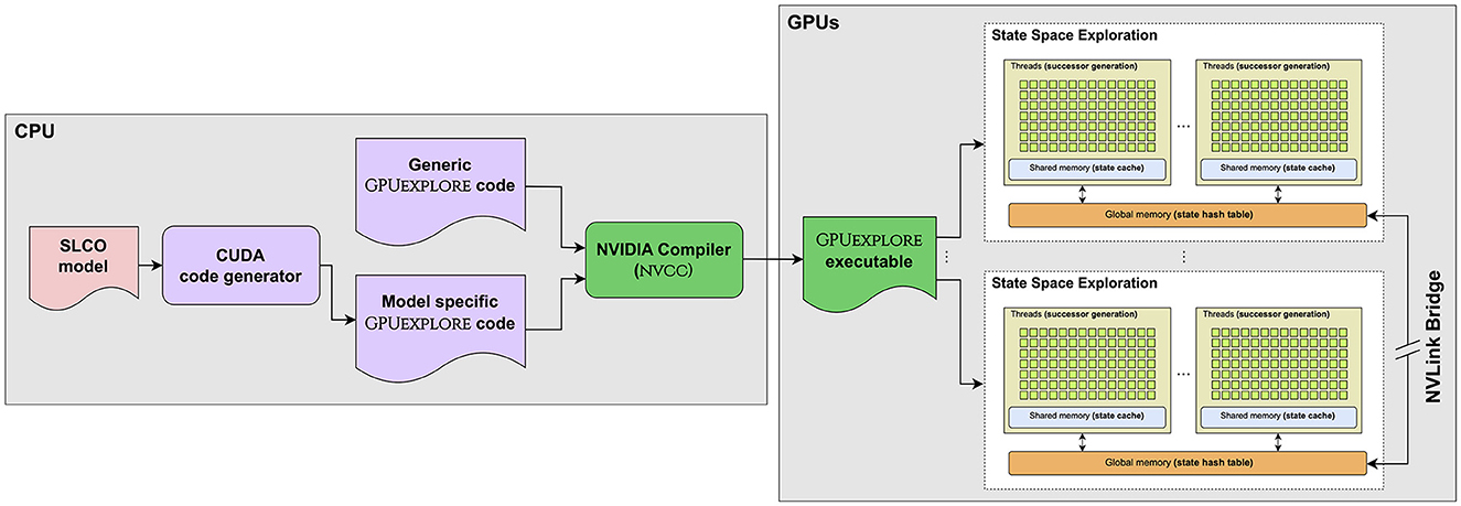
Figure 9. The multi-GPU workflow of GPUEXPLORE 3.0.

As noted in Section 3.3 and Figure 9, the GPUs in a machine can be connected via NVLink bridges, in which case fast peer-to-peer communication is possible. For GPUEXPLORE, this means that the threads of a GPU can access the global memory of all other GPUs. While this simplifies communication between GPUs, there is still a need for a mechanism that distributes the exploration work over the GPUs.

One option would be to use NVIDIA's unified memory, by which the global memories of multiple GPUs can be treated as virtually one address space. This would completely hide the fact that the memory is physically distributed over multiple GPUs. While this is appealing, it also has a drawback for those configurations in which we use a root table and an internal table. In practice, the internal table can be kept relatively small, meaning that it can be expected that this table physically resides in the memory of a single GPU. As a consequence, with unified memory, each time a state tree is retrieved, which happens at high frequency, the memory of that GPU will be accessed. While NVLink is fast, accessing the local global memory is still faster.

For this reason, we opt for a more balanced approach, in which each GPU maintains its own separate hash table(s). This means that when a root table and an internal table are to be used, each GPU has its own root and internal table. A consequence of this is that the exploration algorithm needs to explicitly determine for each state on which GPU it should be stored. This can be done using a hash function, as is done in distributed model checking (see Section 2): For a given set of GPU IDs I, a function h_own:S→I, with S the set of states, is used. Each time a state s is constructed, h_own(s) is the GPU that “owns” s, meaning that s should be stored in the hash table(s) of h_own(s). This makes sure that every state is only stored once in the memory of a single GPU, and it is clear where to search for a given state.

Since multiple internal tables are used when root compression is applied, the state storage procedure is altered to ensure that, for each root stored in the root table of a GPU i, all non-root nodes belonging to the same state tree are stored in the internal table of GPU i. The drawback of this is that non-root nodes may be stored multiple times in different internal tables, i.e., less sharing is achieved, but the important benefit is that trees stored in the hash tables of GPU i can be retrieved by the threads of GPU i without requiring any inter-GPU communication.

This requirement to store all the nodes of a tree in the memory of one particular GPU raises one question: How do we identify the owner of a new tree? This is not trivial. Recall that once all nodes for a new tree have been constructed and stored in the cache of a thread group, FINDORPUT-MANY is called (see Algorithm 3), in which the threads in the group scan the cache and search the encountered nodes in $\mathcal{G}$. At this point, the threads do not distinguish trees. Since trees are stored bottom up, i.e., the leaves are stored first, it must be known, when processing those leaves in FINDORPUT-MANY, to which GPU they belong. In multi-GPU mode, the owner ID is therefore stored in the cache in combination with the cache pointers when a node is constructed, i.e., in terms of Figure 8 inside the gray cells. Since the nodes of a new state tree are constructed bottom up and left to right, the first leaf (counting from the left) is used to identify the owner, in other words; this node is hashed using h_own. As this node always contains the current FSM states of (some of) the FSMs in the input SLCO model, this node is relatively often updated, which helps in hashing the states to different owners, thereby stimulating a balanced work distribution.

We refrain from showing any of the previous algorithms updated for the multi-GPU setting. The only important changes are that owner IDs are stored when new nodes are added to the cache, thereby identifying for each node the GPU it owns. What remains important to note is that even when the threads of one GPU store a new state tree in the memory of another GPU, those threads can still claim that new state for exploration later. Therefore, work distribution across GPUs is flexible in the same way that work distribution among blocks of the same GPU is flexible: if a block still has not accumulated enough work for the next exploration round, it is free to claim its newly generated states for itself. However, the root references in the work tile of a block are assumed to point to states in the global memory of the same GPU. Hence, work claiming can only be done when the current exploration iteration is not the last one of the current EXPLORE kernel call. If it is not the last iteration, the entire state tree already resides in the cache, and therefore, no root reference needs to be used to retrieve the tree, i.e., FETCH does not need to process that tree.

7 Experimental evaluation

We implemented a code generator in PYTHON, using TEXTX (Dejanović et al., 2017) and JINJA2,⁴ that accepts an SLCO model and produces CUDA C++ code to explore its state space. The code is compiled with CUDA 12 targeting compute capability 7.0 on the Tesla V100 and 7.5 on the Titan RTX. To evaluate the runtime and memory performance of GPUEXPLORE 3.0, we conducted two different sets of experiments:

1. Various combinations of hashing techniques are tested on a single GPU and compared to state-of-the-art CPU tools.

2. Based on the results with the experiments, we run the best hashing technique on a setup of one, two, and four GPUs.

7.1 Hashing experiments

For this set of experiments, we used a machine running LINUX MINT 20 with a 4-core INTEL CORE i7-7700 3.6 GHz, 32GB RAM and a Titan RTX GPU with 24GB of global memory, 64KB of shared memory, and 4,607 cores running at 2.1 GHz.

The goal of the experiments is to assess how fast GPU next-state computation using the tree database is with respect to: (1) the various options we have for hashing, (2) state-of-the-art CPU tools, and (3) other GPU tools. For state-of-the-art CPU tools, we compare with 1- and 4-core configurations for the depth-first search (DFS) of SPIN 6.5.1 (Holzmann and Bošnački, 2007) and the (explicit-state) breadth-first search (BFS) of LTSMIN 3.0.2 (Laarman, 2014; Kant et al., 2015). We only enabled state compression and basic reachability (without property checking) to favor fast exploration of large state spaces.

In our implementation, we use 32 invertible hash functions. Root compression (CMP) can be turned on or off. When selected, we have a root table with 2³² elements, 32 bits each and an internal hash table with 2²⁹ elements, 64 bits each. This enables the storage of 58-bit roots (two pointers to the internal hash table) in 58 − 32+⌈log₂(32)⌉+1 = 32 bits. When using buckets with more than one element (CMP+BU), we have root buckets of size 8 and internal buckets of size 16. The internal buckets make full use of the cache line, but the root buckets do not. Making the latter larger means that too many bits for root addressing are lost for root compression to work (the remainders will be too large).

Root compression allows turning cuckoo hashing on (CMP(+BU)+CU) or off (CMP(+BU)). When it is off, compact-multiple-functions hashing is performed, meaning that hashing fails as soon as all possible 32 buckets for a node are occupied.

In the configuration BU, neither root compression nor cuckoo hashing is applied. We use one table with 2³⁰ 64-bit elements and buckets of size 16. For reasons related to storing global addresses in the state cache, we cannot make the table larger. The 32 hash functions are used without allowing evictions, i.e., multiple-functions hashing is applied.

Finally, multiple iterations can be run per kernel launch, as explained in Section 6.6. Shared memory is wiped when a kernel execution terminates, but the state cache content can be reused from one iteration to the next when a kernel executes multiple iterations by which trees already in the cache do not need to be fetched again from the tree database. We identified 30 iterations to be effective in general (i30) and experimented with a single iteration per kernel launch (i1).

For benchmarks, we used models from the BEEM benchmark set (Pelánek, 2007) of concurrent systems, translated to SLCO and PROMELA (for SPIN). We scaled some of them up to have larger state spaces. Those are marked in the tables with “+.” Timeout is set to 3,600 s for all benchmarks.

Figure 10 compares the speeds of the different GPU configurations in millions of states per second, averaged over five runs. For each configuration, we sorted the data to observe the overall trend. The higher the speed the better. The CMP + i30 mode (without cuckoo hashing or larger buckets) is the fastest for the majority of models. However, it fails to complete exploration for at.8, the largest state space with 3.7 billion states, due to running out of memory. If cuckoo hashing is enabled with root compression, all state spaces are successfully explored, which confirms that higher load factors can be achieved (Awad et al., 2023).

Figure 10

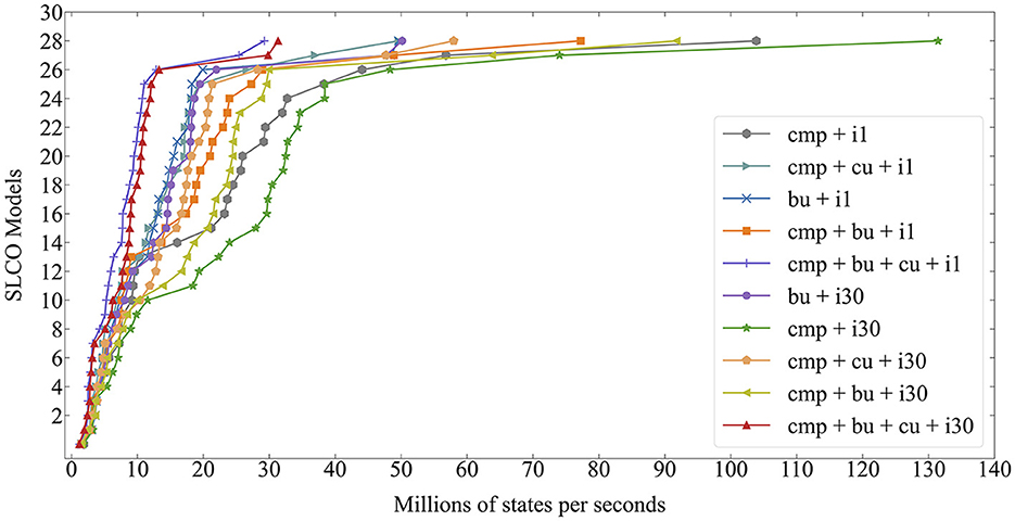
Figure 10. Speed obtained by different GPU configurations.

However, cuckoo hashing negatively impacts performance, which contradicts the findings of Awad et al. (2023). Although it is difficult to pinpoint the cause for this, it is clear that this is caused by our hashing being done in addition to the exploration tasks, while in articles on GPU hash tables (Alcantara et al., 2012; Awad et al., 2023), hashing is analyzed in isolation, i.e., the GPU threads only perform insertions or lookups and are not burdened with additional tasks, such as successor generation, that require additional register variables and instruction steps. With the extra variables and operations needed for exploration, hashing should be lightweight, and cuckoo hashing introduces handling evictions. The more complex code is compiled to a less performant program even when evictions do not occur.

The same can be concluded for larger buckets. Awad et al. (2023) and Alcantara et al. (2012) conclude that larger buckets are beneficial for performance, but for GPUEXPLORE, sacrificing parallelism to achieve more coalesced memory accesses has a negative impact, probably also due to the threads performing much more than only hash tables insertions.

Table 1 compares GPU performance with SPIN and LTSMIN. From the results of Figure 10, we selected a set of configurations demonstrating the impact of the various options. For each model, BITS and CR gives the state vector length in bits and the compression ratio, defined as (number of roots × number of leaves per tree)/(number of nodes). With the compression ratio, we measure how effective the node sharing is compared to if we had stored each state individually without sharing. In addition, the speed in millions of states per second is given. Regarding out of memory, we are aware that SPIN has other, slower, compression options, but we only considered the fastest to favor the CPU speeds. Times are restricted to exploration: code generation and compilation always take a few seconds. The best GPU results are highlighted in bold. To compute the speedup (SU), the result of CMP + i30, the overall best configuration, has been divided by the 1-core LTSMIN result. All GPU experiments have been done with 512 threads per block and 3,240 blocks (45 blocks per SM). We identified this configuration as being effective for anderson.6, and used it for all models.

Table 1

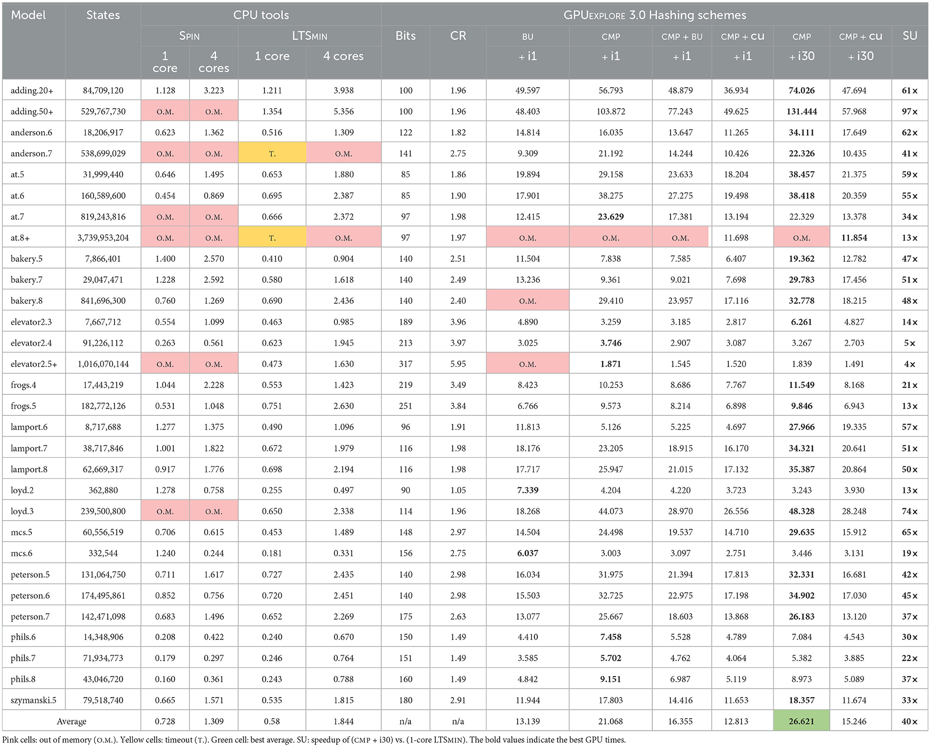
Table 1. Millions of states per second for various reachability tools and configurations.

While LTSMIN tends to achieve near-linear speedups (compare 1- and 4-core LTSMIN), the speed of GPUEXPLORE 3.0 heavily depends on the model. For some models, as the state spaces of instances become larger, the speed increases, and for others, it decreases. The exact cause for this is hard to identify, and we plan to work on further optimisations. For instance, the branching factor, i.e., average number of successors of a state, plays a role here, as large branching factors favor parallel computation (many threads will become active quickly).

Finally, Table 2 compares GPUEXPLORE 3.0 with GPUEXPLORE 2.0 and GRAPPLE. A comparison with PARAMOC was not possible as it targets very different types of (sequential) models. The models we selected are those available for at least two of the tools we considered. Unfortunately, GRAPPLE does not (yet) support reading PROMELA models. Instead, a number of models are encoded directly into its source code, and we were limited to checking only those models. It can be observed that, in the majority of cases, our tool achieves the highest speeds, which is surprising, as the trees we use tend to lead to more global memory accesses, but it is also encouraging to further pursue this direction.

Table 2

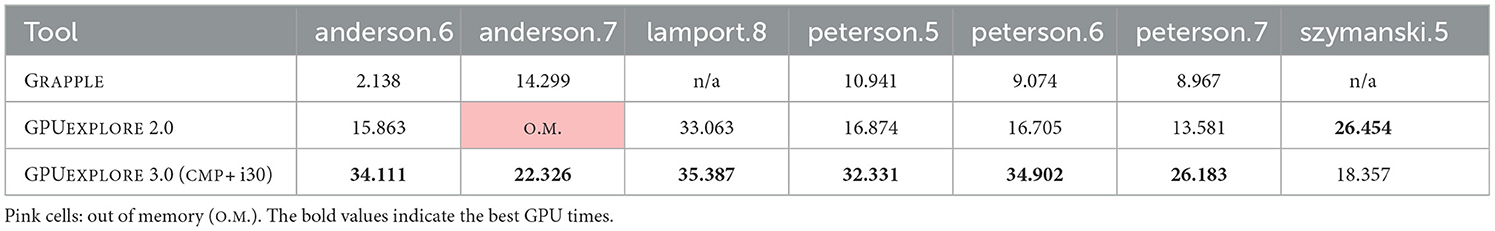
Table 2. Millions of states per second for various GPU tools.

7.2 Multi-GPU experiments

To set up a multi-GPU environment for the experiments, we used an elastic compute cloud (EC2) node running AMAZON LINUX 2 with 4 TESLA V100 GPUs. Each GPU has 16 GB of global memory, 96 KB of shared memory, and 5,120 cores operating at 1.5 GHz clock speed. Multi-core CPU experiments were performed on a different non-GPU node running UBUNTU 22.04 with an Intel Xeon Platinum 8375C having 32 cores operating at 2.9 GHz.

The goal of the experiments is to assess how far a multi-GPU setting can improve the runtime of state space exploration while balancing memory use and the workload, especially for extremely large models that cannot be processed on a single GPU. To this end, we extended our benchmarks with the following new models: peg_solitaire.6, blocks.4, leader_filters.6, anderson.10+, anderson.11+, bakery.9+, and lamport.9+. The + symbol implies the associated models are scaled up. For all multi-GPU experiments, we chose the best performing configuration for the first set of benchmarks (CMP + i30). However, we changed the root table size to 2³¹ to make it fit the V100's global memory of 16GB. The number of invertible hash functions and the size of the non-root table remain the same as in Table 1. Finally, we compare GPUEXPLORE with a 32-core configuration of LTSMIN.

Table 3 shows the speed of GPUEXPLORE (CMP + i30) in millions of states per seconds for different numbers of GPUs and compares it with 32-core LTSMIN. For seven models, exploration failed on a single GPU as it ran out of memory, while the four GPUs setup was capable of fully exploring the state space of all models. Furthermore, a logarithmic acceleration up to 1.9 × was achieved with four GPUs compared to one and two GPUs. We believe that a linear speedup can be easily accomplished with faster P2P communications between the GPUs. Compared to 32-core LTSMIN, GPUEXPLORE with four GPUs achieved speedups of up to 35.6 × ; see the bakery.5 model. With regard to memory footprint, LTSMIN consumes ~30 GB of memory for the largest model, at.8+, whilst GPUEXPLORE only uses ~22 GB of the pre-allocated hash tables on four GPUs.

Table 3

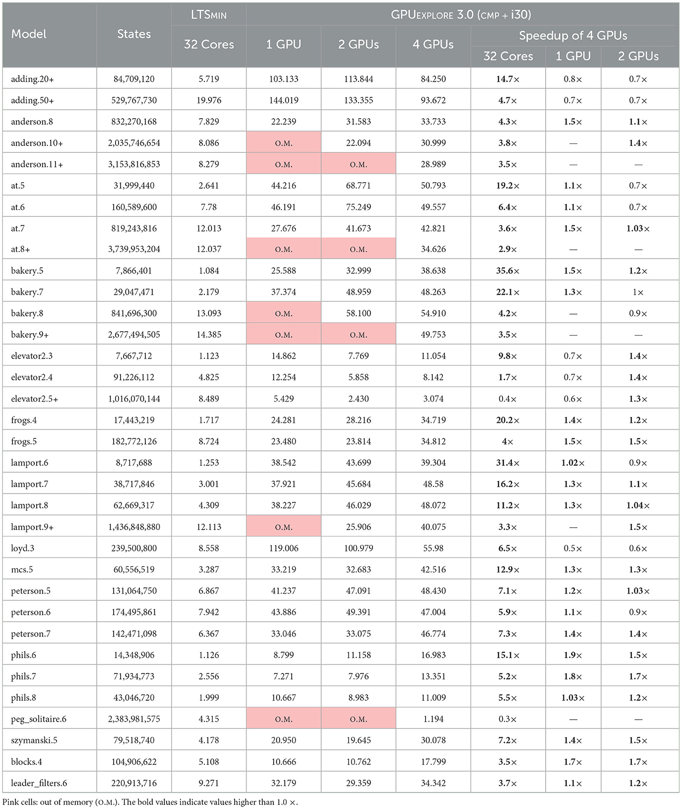
Table 3. Millions of states per second for multi-GPU GPUexplore 3.0 (cmp + i30) and 32-core LTSmin.

Table 4 gives a glance over the workload distribution among multiple GPUs. We conclude that, with n GPUs, each GPU tends to explore 1/nth of the reachable states. This is optimal in terms of load balancing. For many models, GPUEXPLORE ideally distributes states over two and four GPUs, with 50 and 25% of the work being done by each GPU, respectively.

Table 4

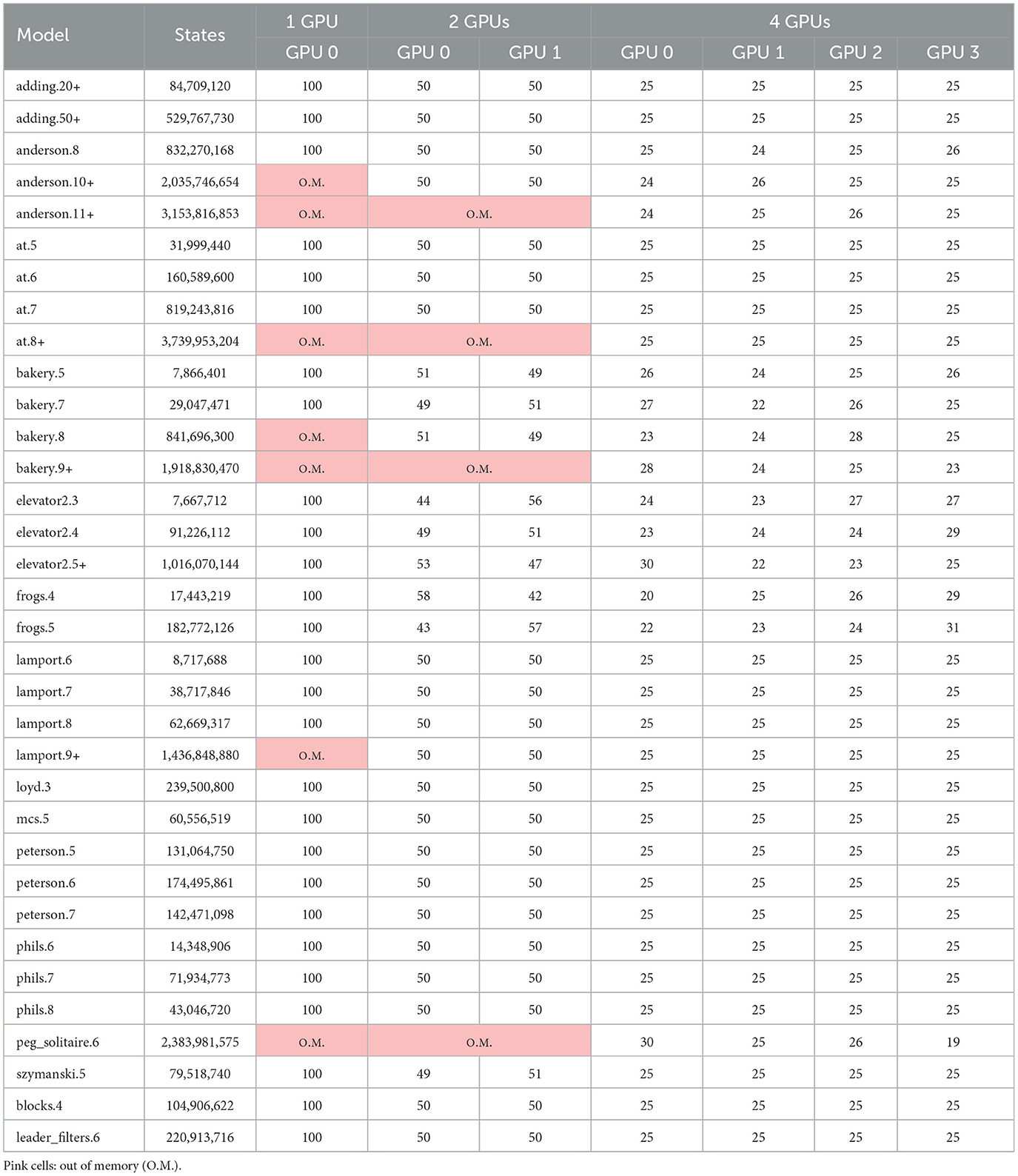
Table 4. Percentage of reachable states discovered over multiple GPUs.

8 Conclusion and future work

In this study, we presented GPUEXPLORE 3.0, which is equipped with a novel GPU tree database. We discussed new algorithms to fetch, generate, and store state trees. This database enables memory-efficient explicit state space exploration for FSMs with data. The new hashing schemes compact-cuckoo and compact-multiple-functions hashing make it possible to use, for the first time, Cleary compression on GPUs. Experiments show processing speeds of up to 144 million states per second.

Furthermore, we extended our implementation to using multiple GPUs, when available, on a single machine. Experiments show that the work and storage distributions are optimal and that the use of four GPUs can improve the performance of GPUEXPLORE up to two times faster than a single GPU with communication overhead taken into account.

In the last decade, new GPUs have been increasingly effective for state space exploration (Cassee et al., 2017), and in the future, they are expected to be more capable of handling thread divergence, which still heavily occurs when accessing the hash tables. Therefore, we are optimistic about further improvements. For the future, we plan to focus on further optimising GPUEXPLORE and adding support for the verification of temporal logic formulae.

Data availability statement

The raw data supporting the conclusions of this article will be made available by the authors, without undue reservation.

Author contributions

AW: Conceptualization, Data curation, Formal analysis, Funding acquisition, Investigation, Methodology, Project administration, Resources, Software, Supervision, Validation, Visualization, Writing—original draft, Writing—review & editing. MO: Data curation, Formal analysis, Investigation, Resources, Software, Validation, Visualization, Writing—original draft, Writing—review & editing.

Funding

The author(s) declare financial support was received for the research, authorship, and/or publication of this article. This study received funding from NWO via grant OCENW.M.21.061 for the GAP project and from Amazon.com, Inc. via an Amazon Research Award (Fall 2021). The funder was not involved in the study design, collection, analysis, interpretation of data, the writing of this article, or the decision to submit it for publication.

Conflict of interest

The authors declare that the research was conducted in the absence of any commercial or financial relationships that could be construed as a potential conflict of interest.

Publisher's note

All claims expressed in this article are solely those of the authors and do not necessarily represent those of their affiliated organizations, or those of the publisher, the editors and the reviewers. Any product that may be evaluated in this article, or claim that may be made by its manufacturer, is not guaranteed or endorsed by the publisher.

Footnotes

1. ^This refers to the single-level version of their cuckoo hashing (Alcantara et al., 2012), which we consider in this research. Their two-level version is more complex and less efficient.

2. ^https://developer.nvidia.com/cuda-zone

3. ^https://palletsprojects.com/p/jinja/

4. ^https://palletsprojects.com/p/jinja/

References

Alcantara, D. A., Volkov, V., Sengupta, S., Mitzenmacher, M., Owens, J. D., Amenta, N., et al. (2012). “Building an efficient hash table on the GPU,” in GPU Computing Gems Jade Edition, ed. W.-M.W. Hwu (Cambridge, MA: Morgan Kaufmann Publishers Inc), 39–53. doi: 10.1016/B978-0-12-385963-1.00004-6

Crossref Full Text | Google Scholar

Amble, O., and Knuth, D. (1974). Ordered hash tables. Comput. J. 17, 135–142. doi: 10.1093/comjnl/17.2.135

Crossref Full Text | Google Scholar

Ashkiani, S., Farach-Colton, M., and Owens, J. (2018). “A dynamic hash table for the GPU,” in IPDPS (New York, NY: ACM), 419–429. doi: 10.1109/IPDPS.2018.00052

Crossref Full Text | Google Scholar

Awad, M., Ashkiani, S., Porumbescu, S., Farach-Colton, M., and Owens, J. (2023). “Analyzing and implementing GPU hash tables,” in APOCS, 2108.07232. (Philadelphia, PA: SIAM), 33–50. doi: 10.1137/1.9781611977578.ch3

Crossref Full Text | Google Scholar

Azar, Y., Broder, A., Karlin, A., and Upfal, E. (1999). Balanced allocations. SIAM J. Comput. 29, 180–200. doi: 10.1137/S0097539795288490

Crossref Full Text | Google Scholar

Baier, C., and Katoen, J. (2008). Principles of Model Checking. Cambridge, MA: MIT Press.

Google Scholar

Barnat, J., Bauch, P., Brim, L., and Češka, M. (2012). Designing fast LTL model checking algorithms for many-core GPUs. JPDC 72, 1083–1097. doi: 10.1016/j.jpdc.2011.10.015

Crossref Full Text | Google Scholar

Barnat, J., Brim, L., Černá, I., Moravec, P., Ročkai, P., and Šimeček, P. (2006). “DIVINE - a tool for distributed verification,” in CAV, Volume 4144 of LNCS, eds T. Ball, and R. B. Jones (Berlin: Springer), 278–281. doi: 10.1007/11817963_26

Crossref Full Text | Google Scholar

Bartocci, E., DeFrancisco, R., and Smolka, S. A. (2014). “Towards a GPGPU-parallel SPIN model checker,” in SPIN 2014 (New York, NY: ACM), 87–96. doi: 10.1145/2632362.2632379

Crossref Full Text | Google Scholar

Behrmann, G., Hune, T., and Vaandrager, F. (2000). “Distributing timed model checking - how the search order matters,” in CAV, Volume 1855 of LNCS, eds E. A. Emerson, and A. P. Sistla (Berlin: Springer), 216–231. doi: 10.1007/10722167_19

Crossref Full Text | Google Scholar

Blom, S., Calamé, J., Lisser, B., Orzan, S., Pang, J., van de Pol, J., et al. (2007). “Distributed analysis with μCRL: a compendium of case studies,” in TACAS, Volume 4424 of LNCS, eds O. Grumberg, and M. Huth (Berlin: Springer), 683–689. doi: 10.1007/978-3-540-71209-1_53

Crossref Full Text | Google Scholar

Blom, S., Lisser, B., van de Pol, J., and Weber, M. (2008). A database approach to distributed state space generation. Electron. Notes Theor. Comput. Sci. 198, 17–32. doi: 10.1016/j.entcs.2007.10.018

Crossref Full Text | Google Scholar

Bošnački, D., Edelkamp, S., Sulewski, D., and Wijs, A. (2011). Parallel probabilistic model checking on general purpose graphics processors. STTT 13, 21–35. doi: 10.1007/s10009-010-0176-4

Crossref Full Text | Google Scholar

Bussi, L., Ciancia, V., and Gadducci, F. (2021). “Towards a spatial model checker on GPU,” in FORTE, Volume 12719 of LNCS, eds K. Peters, and T. A. C. Willemse (Cham: Springer), 188–196. doi: 10.1007/978-3-030-78089-0_12

Crossref Full Text | Google Scholar

Cassee, N., Neele, T., and Wijs, A. (2017). “On the scalability of the GPUexplore explicit-state model checker,” in GaM, Volume 263 of EPTCS (The Hague: Open Publishing Association), 38–52. doi: 10.4204/EPTCS.263.4

Crossref Full Text | Google Scholar

Cassee, N., and Wijs, A. (2017). “Analysing the performance of GPU hash tables for state space exploration,” in GaM, EPTCS (The Hague: Open Publishing Association), 1–15. doi: 10.4204/EPTCS.263.1

Crossref Full Text | Google Scholar

Češka, M., Pilař, P., Paoletti, N., Brim, L., and Kwiatkowska, M. (2016). “PRISM-PSY: precise GPU-accelerated parameter synthesis for stochastic systems,” in TACAS, Volume 9636 of LNCS, eds M. Chechik, and J. F. Raskin (Berlin: Springer), 367–384. doi: 10.1007/978-3-662-49674-9_21

Crossref Full Text | Google Scholar

Ciardo, G., Gluckman, J., and Nicol, D. (1998). Distributed State space generation of discrete-state stochastic models. INFORMS J. Comput. 10, 82–93. doi: 10.1287/ijoc.10.1.82

Crossref Full Text | Google Scholar

Clarke, E. M., Grumberg, O., Kroening, D., Peled, D. A., and Veidt, H. (2018). Model Checking, Second Edition. Cambridge, MA: MIT Press.

Google Scholar

Cleary, J. (1984). Compact hash tables using bidirectional linear probing. IEEE Trans. Comput. c-33, 828–834. doi: 10.1109/TC.1984.1676499

Crossref Full Text | Google Scholar

Cormen, T. H., Leiserson, C. E., Rivest, R. L., and Stein, C. (2009). Introduction to Algorithms, 3rd ed. Cambridge, MA: MIT Press.

Google Scholar

Darragh, J., Cleary, J., and Witten, I. (1993). Bonsai: a compact representation of trees. Softw. Pract. Exper. 23, 277–291. doi: 10.1002/spe.4380230305

Crossref Full Text | Google Scholar

de Putter, S., Wijs, A., and Zhang, D. (2018). “The SLCO framework for verified, model-driven construction of component software,” in FACS, Volume 11222 of Lecture Notes in Computer Science, eds K. Bae, and Ölveczky, P. (Cham: Springer), 288–296. doi: 10.1007/978-3-030-02146-7_15

Crossref Full Text | Google Scholar

DeFrancisco, R., Cho, S., Ferdman, M., and Smolka, S. A. (2020). Swarm model checking on the GPU. Int. J. Softw. Tools Technol. Transf. 22, 583–599. doi: 10.1007/s10009-020-00576-x

Crossref Full Text | Google Scholar

Dejanović, I., Vaderna, R., Milosavljević, G., and Vuković, Ž (2017). TextX: a Python tool for domain-specific language implementation. Knowl.-Based Syst. 115, 1–4. doi: 10.1016/j.knosys.2016.10.023

Crossref Full Text | Google Scholar

Dill, D. (1996). “The Murϕ verification system,” in CAV, Volume 1102 of LNCS, eds R. Alur, and T. A. Henzinger (Cham: Springer), 390–393. doi: 10.1007/3-540-61474-5_86

Crossref Full Text | Google Scholar

Dumas, J.-G. (2014). On Newton-Raphson iteration for multiplicative inverses modulo prime powers. IEEE Trans. Comput. 63, 2106–2109. doi: 10.1109/TC.2013.94

Crossref Full Text | Google Scholar

Edelkamp, S., and Sulewski, D. (2010a). “Efficient explicit-state model checking on general purpose graphics processors,” in SPIN, Volume 6349 of LNCS, eds J. van de Pol, and M. Weber (Berlin: Springer), 106–123. doi: 10.1007/978-3-642-16164-3_8

Crossref Full Text | Google Scholar

Edelkamp, S., and Sulewski, D. (2010b). “External memory breadth-first search with delayed duplicate detection on the GPU,” in MoChArt, Volume 6572 of LNCS, eds R. van der Meyden, and J. G. Smaus (Berlin: Springer), 12–31. doi: 10.1007/978-3-642-20674-0_2

Crossref Full Text | Google Scholar

Garavel, H., Mateescu, R., and Smarandache, I. (2001). “Parallel state space construction for model-checking,” in SPIN, Volume 2057 of LNCS, M. Dwyer (Berlin: Springer), 217–234. doi: 10.1007/3-540-45139-0_14

Crossref Full Text | Google Scholar

García, I., Lefebvre, S., Hornus, S., and Lasram, A. (2011). Coherent parallel hashing. ACM Trans. Graph. 30:161. doi: 10.1145/2070781.2024195

Crossref Full Text | Google Scholar

Holzmann, G. (1997). The model checker spin. IEEE Trans. Softw. Eng. 23, 279–295. doi: 10.1109/32.588521

Crossref Full Text | Google Scholar

Holzmann, G., and Bošnački, D. (2007). The design of a multicore extension of the SPIN model checker. IEEE Trans. Softw. Eng. 33, 659–674. doi: 10.1109/TSE.2007.70724

Crossref Full Text | Google Scholar

Jünger, D., Kobus, R., Müller, A., Hundt, C., Xu, K., Liu, W., et al. (2020). “WarpCore: a library for fast hash tables,” in HiPC (Pune: IEEE), 11–20. doi: 10.1109/HiPC50609.2020.00015

Crossref Full Text | Google Scholar

Kant, G., Laarman, A., Meijer, J., Pol, J. V., Blom, S., and Dijk, T. (2015). “LTSmin: high-performance language-independent model checking,” in TACAS, Volume 9035 of LNCS, eds C. Baier, and C. Tinelli (Berlin: Springer), 692–707. doi: 10.1007/978-3-662-46681-0_61

Crossref Full Text | Google Scholar

Khan, M., Hassan, O., and Khan, S. (2021). “Accelerating SpMV multiplication in probabilistic model checkers using GPUs,” in ICTAC, Volume 12819 of LNCS (Berlin: Springer), 86–104. doi: 10.1007/978-3-030-85315-0_6

Crossref Full Text | Google Scholar

Laarman, A. (2014). Scalable Multi-Core Model Checking [PhD thesis]. Enschede: University of Twente.

Google Scholar

Laarman, A. (2019). Optimal compression of combinatorial state spaces. Innov. Syst. Softw. Eng. 15, 235–251. doi: 10.1007/s11334-019-00341-7

Crossref Full Text | Google Scholar

Laarman, A., van de Pol, J., and Weber, M. (2011). “Parallel recursive state compression for free,” in SPIN, Volume 6823 of LNCS, eds A. Groce, M. Musuvathi (Berlin: Springer), 38–56. doi: 10.1007/978-3-642-22306-8_4

Crossref Full Text | Google Scholar

Lang, F. (2006). “Refined interfaces for compositional verification,” in FORTE, Volume 4229 of LNCS (Berlin: Springer), 159–174. doi: 10.1007/11888116_13

Crossref Full Text | Google Scholar

Lee, C. (1959). Representation of switching circuits by binary-decision programs. Bell Syst. Tech. J. 38, 985–999. doi: 10.1002/j.1538-7305.1959.tb01585.x

Crossref Full Text | Google Scholar

Leiserson, C. E., Thompson, N. C., Emer, J. S., Kuszmaul, B. C., Lampson, B. W., Sanchez, D., et al. (2020). There's plenty of room at the top: what will drive computer performance after Moore's law? Science 368:eaam9744. doi: 10.1126/science.aam9744

PubMed Abstract | Crossref Full Text | Google Scholar

Lerda, F., and Sista, R. (1999). “Distributed-memory model checking with SPIN,” in SPIN, Volume 1680 of LNCS (Berlin: Springer), 22–39. doi: 10.1007/3-540-48234-2_3

Crossref Full Text | Google Scholar

Lessley, B. (2019). Data-parallel hashing techniques for GPU architectures. IEEE Trans. Parallel Distrib. Syst. 31, 237–250. doi: 10.1109/TPDS.2019.2929768

Crossref Full Text | Google Scholar

Merrill, D., and Grimshaw, A. (2011). High performance and scalable radix sorting: a case study of implementing dynamic parallelism for GPU computing. Parallel Process. Lett. 21, 245–272. doi: 10.1142/S0129626411000187

Crossref Full Text | Google Scholar

Neele, T., Wijs, A., Bošnački, D., and van de Pol, J. (2016). “Partial order reduction for GPU model checking,” in ATVA, Volume 9938 of LNCS (Cham: Springer), 357–374. doi: 10.1007/978-3-319-46520-3_23

Crossref Full Text | Google Scholar

Osama, M. (2022). GPU Enabled Automated Reasoning [PhD thesis]. Eindhoven: Eindhoven University of Technology. ISBN: 978-90-386-5445-4.

Google Scholar

Osama, M., Gaber, L., Hussein, A. I., and Mahmoud, H. (2018). An efficient SAT-based test generation algorithm with GPU accelerator. J. Electron. Test. 34, 511–527. doi: 10.1007/s10836-018-5747-4

Crossref Full Text | Google Scholar

Osama, M., and Wijs, A. (2019a). “Parallel SAT simplification on GPU architectures,” in TACAS, Volume 11427 of LNCS (Cham: Springer), 21–40. doi: 10.1007/978-3-030-17462-0_2

Crossref Full Text | Google Scholar

Osama, M., and Wijs, A. (2019b). “SIGmA: GPU accelerated simplification of SAT formulas,” IFM, Volume 11918 of LNCS, eds W. Ahrendt, and S. Tapia Tarifa (Cham: Springer), 514–522. doi: 10.1007/978-3-030-34968-4_29

Crossref Full Text | Google Scholar

Osama, M., and Wijs, A. (2021). “GPU acceleration of bounded model checking with ParaFROST,” in CAV, Part II, Volume 12760 of LNCS, eds A. Silva, and K. R. M. Leino (Cham: Springer), 447–460. doi: 10.1007/978-3-030-81688-9_21

Crossref Full Text | Google Scholar

Osama, M., Wijs, A., and Biere, A. (2021). “SAT solving with GPU accelerated inprocessing,” in TACAS, volume 12651 of LNCS, eds J. F. Groote, and K. G. Larsen (Cham: Springer), 133–151. doi: 10.1007/978-3-030-72016-2_8

Crossref Full Text | Google Scholar

Osama, M., Wijs, A., and Biere, A. (2023). Certified SAT solving with GPU accelerated inprocessing. Form Methods Syst Des. 133–151. doi: 10.1007/s10703-023-00432-z

Crossref Full Text | Google Scholar

Pagh, R., and Rodler, F. F. (2001). “Cuckoo hashing,” in ESA, Volume 2161 of LNCS, ed. F. M. auf der Heide (Berlin: Springer), 121–133. doi: 10.1007/3-540-44676-1_10

Crossref Full Text | Google Scholar

Pelánek, R. (2007). “BEEM: benchmarks for explicit model checkers,” in SPIN 2007, Volume 4595 of LNCS (Berlin: Springer), 263–267.

Google Scholar

Prevot, N., Soos, M., and Meel, K. (2021). “Leveraging GPUs for effective clause sharing in parallel SAT solving,” in SAT, Volume 12831 of LNCS, eds C. M. Li, and F. Manyà (Cham: Springer), 471–487. doi: 10.1007/978-3-030-80223-3_32

Crossref Full Text | Google Scholar

Saad, Y. (2003). Iterative Methods for Sparse Linear Systems, 2nd ed. Philadelphia, PA: SIAM. doi: 10.1137/1.9780898718003

Crossref Full Text | Google Scholar

van der Vegt, S., and Laarman, A. (2011). “A parallel compact hash table,” in MEMICS, Volume 7119 of LNCS, eds Z. Kotásek, J. Bouda, I. Černá, L. Sekanina, T. Vojnar, and D. Antoš (Berlin: Springer), 191–204. doi: 10.1007/978-3-642-25929-6_18

Crossref Full Text | Google Scholar

Wei, H., Chen, X., Ye, X., Fu, N., Huang, Y., Shi, J., et al. (2018). “Parallel model checking on pushdown systems,” in ISPA/IUCC/BDCloud/SocialCom/SustainCom (Melbourne, VIC: IEEE), 88–95. doi: 10.1109/BDCloud.2018.00026

Crossref Full Text | Google Scholar

Wei, H., Ye, X., Shi, J., and Huang, Y. (2019). “ParaMoC: a parallel model checker for pushdown systems,” in ICA3PP, Volume 11945 of LNCS, eds S. Wen, A. Zomaya, and L. T. Yang (Cham: Springer), 305–312. doi: 10.1007/978-3-030-38961-1_26

Crossref Full Text | Google Scholar

Wijs, A. (2016). “BFS-based model checking of linear-time properties with an application on GPUs,” in CAV, Part II, Volume 9780 of LNCS, eds S. Chaudhuri, and A. Farzan (Cham: Springer), 472–493. doi: 10.1007/978-3-319-41540-6_26

Crossref Full Text | Google Scholar

Wijs, A., and Bošnački, D. (2012). “Improving GPU sparse matrix-vector multiplication for probabilistic model checking,” in SPIN, Volume 7385 of LNCS, eds A. Donaldson, and D. Parker (Berlin: Springer), 98–116. doi: 10.1007/978-3-642-31759-0_9

Crossref Full Text | Google Scholar

Wijs, A., and Bošnački, D. (2014). GPUexplore: many-core on-the-fly state space exploration using GPUs,” in TACAS, Volume 8413 of LNCS, eds E. Ábrahám, and K. Havelund (Berlin: Springer), 233–247. doi: 10.1007/978-3-642-54862-8_16

Crossref Full Text | Google Scholar

Wijs, A., and Bošnački, D. (2016). Many-core on-the-fly model checking of safety properties using GPUs. STTT 18, 169–185. doi: 10.1007/s10009-015-0379-9

Crossref Full Text | Google Scholar

Wijs, A., Katoen, J.-P., and Bošnački, D. (2016a). Efficient GPU algorithms for parallel decomposition of graphs into strongly connected and maximal end components. Formal Methods Syst. Des. 48, 274–300. doi: 10.1007/s10703-016-0246-7

Crossref Full Text | Google Scholar

Wijs, A., Neele, T., and Bošnački, D. (2016b). “GPUexplore 2.0: unleashing GPU explicit-state model checking,” in FM, Volume 9995 of LNCS, eds J. Fitzgerald, C. Heitmeyer, S. Gnesi, and A. Philippou (Cham: Springer), 694–701. doi: 10.1007/978-3-319-48989-6_42

Crossref Full Text | Google Scholar

Wijs, A., and Osama, M. (2023a). “A GPU tree database for many-core explicit state space exploration,” in TACAS, Part I, Volume 13993 of LNCS, eds S. Sankaranarayanan, and N. Sharygina (Cham: Springer), 684–703. doi: 10.1007/978-3-031-30823-9_35

Crossref Full Text | Google Scholar

Wijs, A., and Osama, M. (2023b). “GPUexplore 3.0: GPU accelerated state space exploration for concurrent systems with data,” in SPIN, Volume 13872 of LNCS (Cham: Springer), 188–197. doi: 10.1007/978-3-031-32157-3_11

Crossref Full Text | Google Scholar

Wu, Z., Liu, Y., Liang, Y., and Sun, J. (2014). GPU accelerated counterexample generation in LTL model checking,” in ICFEM, Volume 8829 of LNCS, eds S. Merz, and J. Pang (Cham: Springer), 413–429. doi: 10.1007/978-3-319-11737-9_27

Crossref Full Text | Google Scholar

Wu, Z., Liu, Y., Sun, J., Shi, J., and Qin, S. (2015). “GPU accelerated on-the-fly reachability checking,” in ICECCS (Pune: IEEE), 100–109. doi: 10.1109/ICECCS.2015.21

Crossref Full Text | Google Scholar

Youness, H., Osama, M., Hussein, A., Moness, M., and Hassan, A. M. (2020). An effective SAT solver utilizing ACO based on heterogenous systems. IEEE Access 8, 102920–102934. doi: 10.1109/ACCESS.2020.2999382

Crossref Full Text | Google Scholar

Youness, H. A., Ibraheim, A., Moness, M., and Osama, M. (2015). “An efficient implementation of ant colony optimization on GPU for the satisfiability problem,” in PDP (Turku:IEEE), 230–235. doi: 10.1109/PDP.2015.59

Crossref Full Text | Google Scholar