Transparent, simple and robust fast-and-frugal trees and their construction

Introduction

When a doctor—let's call her Dr. Devlin—decides on a course of treatment for a patient, she coordinates information from multiple sources: the patient's appearance, findings from an examination, test results, the medical history, and so forth. This information constitutes a set of cues, or features, that she uses to make her diagnosis, that is, to classify this case: is the patient diabetic? Do they suffer from hypertension? Do they have COVID? Dr. Devlin uses that classification to make crucial decisions about treatment.

Sometimes, the information at the doctor's disposal may be scarce and the time for action may be limited. But Dr. Devlin's decision making must always be consistent and justifiable. She must be able to explain to patients and colleagues how the available evidence led to her decisions—decisions that follow from the way she classifies each case.

Standardized classification methods have gained importance in the biomedical diagnostic field. Recently, Lötsch (2022) have published a comprehensive review of methods from Artificial Intelligence that are used in the biomedical context for the support of medical diagnosis. The authors report how physicians are now often aided by machine learning algorithms that are designed to produce optimal or near-optimal predictions. The algorithms cover a wide range of models, sometimes denoted “skill learning methods”, such as artificial neural networks, CART, Bayesian Networks and support vector machines. The review demonstrates how an adequate understanding of these methods requires a basic knowledge of statistics and computer science. This has important consequences for the curricula of future doctors.

Unfortunately, as the authors point out, it is often hard for patients (and some practitioners) to understand the explanations given by the developers of the models. One result has been that the traditional doctor-patient relationship, based on trust built through the years, is giving way to a less transparent interaction, in which the doctor communicates diagnostic results obtained by such AI algorithms. These methods are sometimes criticized as being neither easily explainable nor transparent.

We agree with that criticism. Complex machine learning methods for medical diagnosis are guided by a search for optimality or near optimality, often leading to intractability, lack of transparency and lack of explainability. At the other extreme of the spectrum are transparent models such as fast-and-frugal trees, which are guided by a desire for simplicity and transparency, and yet do not have to trade that simplicity for accuracy. They satisfice rather than optimize, that is, they take the perspective of bounded rationality. The essence of bounded rationality is that it results from adaptation between the environment and the mind, and takes advantage of this adaptation (Gigerenzer et al., 1999).

Fast-and-frugal heuristics for medical diagnosis, prediction and decision making have been developed, aiming at modeling and supporting medical institutions and doctors (see, for instance, Green and Mehr, 1997; Fischer et al., 2002; Jenny et al., 2013). In several studies, it has been found that diagnosis based on fast-and-frugal trees is more accurate, especially when generalizing from small training sets to large test sets, than both the physicians' clinical judgment and more complex statistical or machine learning models (Green and Mehr, 1997; Fischer et al., 2002; Jenny et al., 2013).

We introduce fast-and-frugal classification trees and want to compare the efficiency, diagnostic power and accuracy of these trees, which are simple both in construction and execution, with inference machines constructed by other tools. We will exhibit tree-construction tools based on elementary computations of sensitivities and predictive values, produced using the Common Online Data Analysis Platform (CODAP), a free, web-based educational tool for data analysis.

By proposing AI tools based on boundedly rational heuristic models for categorization, classification and decision, we take into account psychological and philosophical principles that have evolved over millennia. We recall that the classical view of categories was introduced in the work of Plato and systematized by Aristotle, whose method was popularized in the Middle Ages through Porphyry's Isagogé. Porphyry's tree is one of the first trees used as a model for categorization and classification. The historical evolution of such trees has been impressive in many realms of human knowledge. Boundedly rational classification trees combine the tree structure with lexicographic procedures, as we will describe below.

These principles help create explainable and transparent tools. Because these heuristics have a small number of parameters, they tend not to overfit, and they compete well with sophisticated machine learning techniques. The overfitting and lack of robustness of complex AI algorithms in the clinical domain has recently been a subject in Stat+ with a detailed account by Casey Ross (2022), which also appeared as this paper was in production¹.

The posture of the paper by Lötsch (2022), may seem extreme. Another perspective may be that the patient trusts the doctor to choose the best option/method. Thus it is actually the doctor who needs to trust the AI; and if they do not, they will be reluctant to apply it, or suggest it to patients. Better, more humane explanations might be a solution in certain circumstances. There is a vivid discussion in the literature with many publications outlining that in certain cases, to generate patient trust, a validated performance might be preferable over explanations [see, for instance, (Katsikopoulos et al., 2021)].

The following section is a brief digression devoted to the main tenets of bounded rationality and their history.

Brief historical account of bounded rationality for decision making

The modern behavioral interpretation that can be formulated in favor of bounded rationality is as follows:

Decisions can be rational or not based on their cognitive success in problem-solving and in adapting to the environment (Gigerenzer and Selten, 2002). According to this ecological perspective, the structure surrounding the decision-making task is highlighted in the process and becomes a fostering factor of succesful procedures. Based on this principle it is preferable, from an adaptive perspective, to adopt heuristic decision-making procedures based on the “less-is-more” principle, and on “satisficing” rather than to search for optimal classifications and decisions. The evolution of bounded rationality as a paradigm had its focus on procedural features. Bounded rationality concerns the process for arriving at a decision, not just the decision itself. It involves substantive rationality, i.e., the rationality of the decision, and also procedural rationality. Taking into account that we live in a world full of uncertainty and cognitive complexity and that humans have limited information processing capacities, Simon (1978, p. 9) introduced the distinction between substantive and procedural rationality in the following way: “In such a world, we must give an account not only of substantive rationality—the extent to which appropriate courses of action are chosen—but also procedural rationality—the effectiveness, in the light of human cognitive powers and limitations, of the procedures used to choose actions.” And Simon remarked that “There is a close affinity between optimizing and substantive rationality, and an affinity between bounded and procedural rationality. The utility-maximizing optimum is independent of the choice process; the outcome is all that counts. In the bounded rationality approach the choice depends upon the process leading up to it” (Simon, 2001). Bounded rationality postulates procedures that respect human limits on knowledge of present and future, on abilities to calculate the implications of knowledge, and on abilities to evoke relevant goals (Simon, 1983). Bounded rationality is thus aimed at attaining outcomes that satisfice (attain aspirations) for the wants and needs that have been evoked (Conlisk, 1996). Procedural rationality stresses the emphasis on the rational scrutiny to which the used procedures can be subjected (Viale, 2021a,b,c). The role of procedural rationality is evident in all the fields of decision making. For example in design and engineering: “Needless to say that, given the uncertainty and cognitive complexity of many engineering-design projects, this form of rationality may be of great importance for engineering-design practice” (Kroes et al., 2009).

Bounded rationality and medical decision-making

Medical classifications deal with the most important of our resources: health. Whether assigning a patient with worrying symptoms to a hospital bed or to her/his home bed, has to be resolved quickly, on the basis of tests and symptoms. During the last 2 years doctors in the world have had to assess the predictive value or diagnostic power of a combination of features and decide accordingly, whether a patient with Covid symptoms has to be assigned to a hospital bed. A decision tree that cristallized from statements from a number of doctors in the city of Tübingen was the following:

What mattered here was making a quick decision. In more standardized procedures some formalization becomes necessary. The high predictive value for an oxygen saturation of <90 (or, in some cases, <85), for high Covid risk had been assessed collectively based on shared knowledge and shared expertise. Low blood pressure was also considered predictive of imminent high risk. Here three features are combined for judgment.

Performing judgment and decision problems by inferences based on situational features is fundamental; what is so special about our mind/brain is that it has, among its competencies, the ability to extract adequate crucial features of items or situations and make predictions based on these features.

From the perspective of AI the construction of the representation scheme for inference corresponds to the extraction of features and the structuring of these features. Trees offer one way of structuring features. Once the features are extracted they have to be organized as a scheme. We combine the Bayesian inference mechanisms with very simple trees. In the next section we begin by discussing about the assessment of predictive values of single cues based on Bayesian inference.

The mathematical tools for accurate inferences in the medical domain

The revolution in the field of medical inferences and classifications came with the formalization of measures for the reliability of the observed features. The most important formalization came with the inception of the probability calculus during the Enlightenment.

Here we make a brief historical digression and recall the origins of the probabilistic calculus: Probability theory emerged during the Enlightenment as tools of rational belief and for decision-making in the presence of risk (Daston, 1995). According to Laplace,

“the theory of probabilities is nothing but common sense reduced to a calculus; it enables us to appreciate with exactness that which accurate minds feel with a sort of instinct for which often they are unable to account,” (Laplace, 1812).

The theory of probabilities made it possible to assess features' reliability, and opened the gate to optimality of judgment and fully rational decision making. Bayes' Theorem, discovered by reverend Thomas Bayes in the eighteenth century, became the tool for assessing predictive values of features.

The enthusiasm of the Enlightenment was crowned by Kolmogorov's embedding of the theory of probability into the axiomatic edifice of modern Mathematics in the early twentieth century (1936). However, in the second half of the twentieth century, the cognitive and behavioral sciences produced a flurry of research demonstrating systematic ways in which human reasoning fails to conform to the probability calculus (Kahneman et al., 1982). The revelation which resolved this gridlock was that the representation of information plays a fundamental role in probabilistic reasoning: representation formats based on a boundedly rational perspective—away from strict formalism—foster probabilistic inferences while formal probabilities blur intuition.

Assessing the predictive value of a feature the Bayesian way

Although Bayesian reasoning can be used for assessing the predictive value of any feature on any item we encounter in everyday life, let us concentrate on the medical domain and consider the following example.

Assume a physician has to establish whether a patient suffers from a disease D based on just one piece of evidence E, which could be, for instance, a symptom or a test result.

During her years of study and experience the physician acquires knowledge on the prior probability, or base rate, of the disease, which can be denoted by P(D+). Here D+ indicates the actual presence of the disease. Assume the piece of evidence is a test T, which can turn out positive, denoted by T+, or negative, denoted by T-. Assume also, that the doctor knows the sensitivity of the test, that is P(T+|D+) and its specificity, that is P(T-|D-). What Bayes‘ Theorem provides is a formula for obtaining P(D+|T+) from these quantities:

$\begin{array}{l}P(D+|T+)=\frac{P(D+)P(T+|D+)}{P(D+)P(T+|D+)+P(D-)P(T+|D-)}\end{array}$

An important mathematical issue is the following: This formula, which is a simple consequence of the definition of conditional probability, contains P(D+), that is the prior probability of the disease being present, in its numerator. This has as consequence that this prior probability has a strong impact on the overall predictive value of the piece of evidence.

As mentioned above, people are notoriously bad at manipulating formal probabilities, as a plethora of empirical studies have shown (Eddy, 1982) and this is typically a problem in the context of medical diagnosis. In Eddy's classical study on doctors' estimate of the probability that a certain disease is present, given that a test of the disease is positive (Eddy, 1982), he discovered that his participants made mistakes based on misconceptions. The so-called predictive value of the test was estimated as being close to the chances of the test detecting the disease. Thus, if a test had a probability of 95% of detecting the disease, Eddy's participants estimated that the actual chances of having the disease, given that the result of the test was positive, was a value quite close to 95%. What surprised Eddy was that the doctors' estimates of P(D+|T+), i.e., the chances of being ill with the disease, given that the test is positive, remained quite close to the inverse probability P(T+|D+), i.e., that the test is positive given that they have the disease, also called sensitivity of the test. Further, they made this error even when the base rate of the disease was very small. As the base rate is found in the numerator, it has a big influence on the result. Therefore, when the disease is very rare, the posterior probability, namely the test's positive predictive value (PPV), tends to be small. This discovery led to a sequence of important replications with the same discouraging results. The key factor that makes this kind of reasoning difficult—even for experts, as Gigerenzer and Hoffrage (1995) pointed out—seems to be the abstract, symbolic format of the 'probabilistic' information used for inference. In the next section, we will present representations and visual aids that simplify the understanding of that same information (again, focussing mainly on examples from medicine).

Boundedly rational representational tools for assessing the quality of features for classification

Being of such fundamental importance Bayesian Reasoning has been studied by cognitive psychologists, who have devised more adaptive information formats for it. A boundedly rational approach has helped translating the formula above in understandable, simple expressions, which are mathematically not equivalent to the formula but help making the adequate classifications. Instead of working with Kolmogorov probabilities the physician can imagine a population of fictitious people, say 1,000 of them. She divides them into those who do and do not have the disease. For example, if the disease is present in only 1% of the population, she would partition her imaginary 1,000 patients into 10 who have the disease and 990 who do not. Of those who have the disease, suppose 80% will test positive. In this case, the doctor imagines that 8 of the 10 ill patients will test positive and 2 will test negative. Now, suppose that 90% of those who do not have the disease will have a negative test result. In our doctor's imaginary population, this works out to 99 healthy patients who test positive and 891 who test negative. The proportions thus formed, 10 out of 1,000, 8 out of 10, 2 out of 10, can easily become part of the computation that leads to an estimate of P(D+|T+), namely 8 out of 107.

Already in this simple situation of just one feature for classification a tree as in Figure 1, becomes a handy, transparent representational aid for depicting the quantitative facts.

FIGURE 1

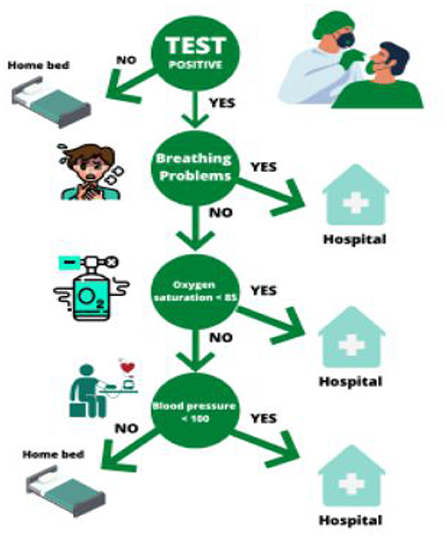
Figure 1. This decision tree summarizes the steps taken to establish whether a patient had to be assigned to a hospital bed during the Covid pandemic.

Natural frequencies appear to be more akin to the unaided mind than formalized probabilities. The approach through natural frequencies is to be seen as “boundedly rational”, because it restricts the reasoning to an imagined fixed finite sample, thus reducing the power of generality of formal probabilities. However, what matters from the perspective of bounded rationality, is that this approach induces people of all ages to make correct inferences. Strict Bayesians criticize natural frequencies because, as Howson and Urbach write in their famous book on scientific reasoning (Howson and Urbach, 1989, 2006), “there is no connection between frequencies in finite samples and probabilities”. Gage and Spiegelhalter (2016) adopt another perspective: they close the gap between probabilities and natural frequencies, by treating natural frequencies as expected frequencies.

Educational tools for fostering proto-Bayesian reasoning based on one feature

During the Covid pandemic the media communicate intermittently data about the incidence or base rate of the disease; less frequently they also describe the sensitivity of tests and their specificity. What matters is then to develop an understanding for positive and negative predictive values as function of sensitivity and specificity, and grasp the changes of the positive and negative predictive value of tests, based on the changes of the disease incidence.

We have developed dynamic webpages, which foster precisely these competencies. Our treatment is based on icon arrays representing data on tests and incidences.

An icon array is a form of pictograph or graphical representation that uses matrices of circles, squares, matchstick figures, faces, or other symbols to represent statistical information. Arrays are usually constructed in blocks, say, of 10, 20, 25, 50, 100, or 1,000 icons where each icon represents an individual in a population. Icons are distinguished by color, shading, shape or form to indicate differences in the features of the population, such as the presence (or absence) of a positive test. In Figure 3 an icon array represents a population of 100 patients, who have made a test for detecting whether they suffer from a disease.

FIGURE 2

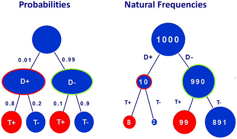
Figure 2. The tree on the left hand side represents information about base rate of the diesease (P(D+) = 0.01), sensitivity of the test P(T+|D+) = 0.8, probability of false negatives (P(T-|D+) = 0.2), probability of false positives (P(T+|D-) = 0.1) and specificity (P(T-|D-) = 0.9). The tree on the right hand side represents the corresponding natural frequencies for a random sample of 1,000 people.

FIGURE 3

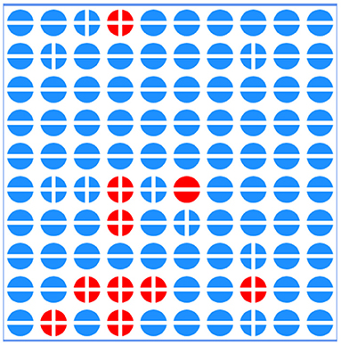
Figure 3. In this array 100 patients are represented by round icons. A red icon represents a patient with the disease, while a blue icon corresponds to a healthy patient. The signs + and – represent positive and negative tested patients.

Icon arrays are helpful for communicating risk information because they draw on people's natural disposition to count (Dehaene, 1997), while also facilitating the visual comparison of proportions (Brase, 2008). Further, the one-to-one match between individual and icon has been proposed to invite identification with the individuals represented in the graphic to a greater extent than other graphical formats (Kurz-Milcke et al., 2008). The next Figure 4 results from sorting the icon array of Figure 3 so that positive tests are grouped together.

FIGURE 4

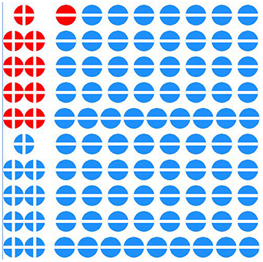
Figure 4. Here the icon array presents the same data as in Figure 2, but they have been sorted, so as to make computations of sensitivity, specificity and predictive values simple.

Figure 4 above shows data from the same 100 people, grouping those who test positive, together by using a button at the bottom of the array.

Icon arrays are excellent tools for representing information but their effectiveness can be enhanced: they can be constructed to be dynamic and interactive. Dynamic displays of icon arrays can be designed in a way that fosters elementary statistical literacy in general. The dynamic aspect may be conferred by sliders that let the agent to modify base rates and population sizes. The additional statistical action is to organize the data so that inference becomes straightforward. In this situation we have two types of inference: one is causal, the other one is diagnostic. In the causal direction the original sample of 100 people splits into the portion with the disease and the portion without the disease. These again split into those with positive and those with negative tests. In the diagnostic direction the first splitting corresponds to the test: those with a positive test and those with a negative one. The next splitting correponds to the disease: present or absent. In order to foster Bayesian inference we arrange these two trees, one causal and one diagnostic into what we call “double tree” as illustrated in Figure 5.

FIGURE 5

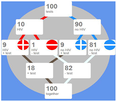
Figure 5. A double tree representing the same data as Figure 3, but organized in a double tree.

Instruction on Bayesian inference based on natural frequencies can be aided by the interactive tool in http://www.eeps.com/projects/wwg/wwg-en.html, developed for this and other purposes by the first and second author.

The QR Code below leads to this interactive page.

The resource is designed for facilitating the teaching and training of basic components of inference and decision making; it by offers multiple complementary and interactive perspectives on the interplay between key parameters. Useful interactive displays for adults have also been introduced, for instance, by Garcia-Retamero et al. (2012).

Trees for inference based on many cues

The advantages of trees with natural frequencies are lost when many cues are considered: As the number of cues grows the size of the natural frequency tree explodes and ecological rationality disappears. Massaro argued in 1998 (Massaro, 1998, p. 178) “a frequency algorithm will not work” because “it might not be reasonable to assume that people can maintain exemplars of all possible symptom configurations”. Based on two cues, as shown by Hoffrage et al. (2015), people are still able to make correct Bayesian inferences. As an example of such a tree consider the one in Figure 6.

FIGURE 6

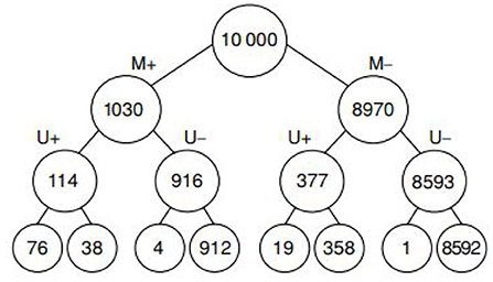
Figure 6. This is a diagnostic tree for classifying patients with breast cancer based on two cues: Mammogramm, labeled by M+ (positive) and M- (negative), Ultrasound test, labeled U+ (positive) and U- (negative). The leaves at the bottom correspond to cancer/no cancer.

But Massaro's view is right when the number of cues grows. The question is then: How can such full trees be pruned or reduced in adequate ways? We discuss two categories of trees for classification and decision-making.

Classification trees

Classification Trees have been used as representational schemes since ancient times; Porphyry used tree based classification already in the years 268–270 in his Isagoge, an introduction to Aristotle's “Categories”. Without digging into details of the fascinating history of trees for knowledge representation and classification we would like to stresss that they have maintained their important role in many realms of science, cognition and machine learning.

In the eighties Breiman et al. introduced the CART algorithm 1993, which has become a popular tool in machine learning. Trees are intuitive, conceptually easy to comprehend and result in nice representations of highly complex datasets. CART forms a milestone in the development of tree methods in function estimation and its applications. CART is based on a generic binary decision tree which proceeds by recursively subdividing the sample space into two sub-parts and then calculating locally an average, trimmed average, median etc. Over the last 30 years, several alternatives to CART have been proposed. Reviews some widely available algorithms and compares their capabilities, strengths and weaknesses.

The construction of trees in regression and classification is based on recursive partitioning schemes (RPS). They proceed by partitioning the sample space into finer sets aiming at having homogeneity according to given criteria. The partitioning scheme is associated with a binary tree. The nodes of the tree correspond to partition sets. If the set is divided into two parts in the process of recursive partitioning, then the corresponding node has two further child nodes. The terminal nodes of a tree correspond to final partition sets and are called leaves.

CART obviously belongs to the realm of unbounded rationality. At the other extreme of the spectrum we find fast-and-frugal trees, which we introduce in the following section.

Boundedly rational fast-and-frugal trees

A fast-and-frugal tree has a single exit at every level before the last one, where it has two. The cues are ordered by means of very simple ranking criteria. Fast-and-frugal trees are implemented step by step, with a limited memory load and can be set up and executed by the unaided mind, requiring, at most, paper and pencil. These paper and pencil computations can be long but elementary.

A fast-and-frugal tree does not classify optimally when fitting known data. It rather “satisfices”, producing good enough solutions with reasonable cognitive effort. For generalization, that is learning their strauctural parameters structure from training sets and extrapolating to test sets, fast-and-frugal trees have proven surprisingly robust. The predictive accuracy and the robustness of the fast-and-frugal tree has been amply demonstrated (Luan et al., 2011; Woike et al., 2017; Martignon and Laskey, 2019).

Martignon, Vitouch, Takezawa and Forster provided a characterization of these trees in 2003:

Theorem: For binary cues with values 0 or 1, a fast-and-frugal tree is characterized by the existence of a unique cue profile of 0's and 1's that operates as a splitting profile of the tree; this means that any item with a profile lexicographically lower than the splitting profile will be classified in one of the two categories, while the rest of items will be classified in the other one, as illustrated in Figure 7.

FIGURE 7

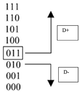
Figure 7. An example of splitting profile characterizing a fast-and-frugal tree for classifying items into two complementary categories based on three cues (extracted from Martignon et al., 2003).

Simple methods for constructing inference trees

The basic elements for making a binary classification are the cues or features, which are here assumed to be binary. In a fast-and-frugal tree, the cues are ranked according to a previously fixed rule. We will treat this ranking phase below. Once the cues are ranked, the tree has one cue at each level of the tree and an exit node at each level (except for two exit nodes for the last cue at the last level of the tree). Every time a cue is used, a question is asked concerning the value of the cue. Each answer to a question can immediately lead to an exit, or it can lead to a further question and eventually to an exit. A fundamental property of fast-and-frugal trees is that, for each question, at least one of the two possible answers leads to an exit.

The execution phase is simple: To use a fast-and-frugal tree, begin at the root and check one cue at a time. At each step, one of the possible outcomes is an exit node which allows for a decision (or action): if an exit is reached, stop; otherwise, continue until an exit is reached. you take an exit, stop; otherwise, continue and ask more questions until an exit is reached.

Figure 8 illustrates a fast-and-frugal tree for classifying a patient as “high risk” of having a heart attack and thus having to be sent to the “coronary care unit” or as “low risk” and thus having to be sent to a “regular nursing bed” (Green and Mehr, 1997). The accuracy and robustness of fast-and-frugal trees has been shown to be comparable to that of Bayesian benchmarks in studies by Martignon and Laskey (2019). Extensive studies comparing the performance of fast-and-frugal trees to that of classification algorithms used in statistics and machine learning, such as Naive Bayes, CART, random forests, and logistic regression, have also been carried out by using large batteries of real-world datasets.

FIGURE 8

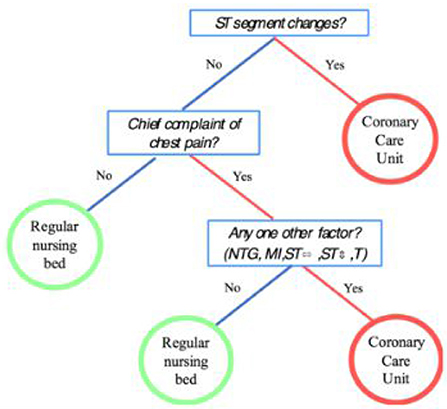
Figure 8. A fast-and-frugal tree for patients with symptoms that may indicate the risk of heart attack.

Constructing fast-and-frugal trees with ARBOR

Arbor is an educational tool for constructing classification trees. It works within CODAP, that is, a user with data in CODAP can use Arbor to construct a tree. An appropriate dataset consists of a collection of cases, represented as rows in a table. The columns of the table are features or attributes of the cases. One of these is the outcome condition that we are trying to predict; we can use the rest as predictors.

Arbor does not compute an optimal tree or use any algorithm. Instead, the user dynamically constructs arbitrary binary trees by dragging attributes (features) onto nodes; Arbor splits that node into two branches, thus growing the tree. One can also “prune” the tree, eliminating nodes. The user also assigns a diagnosis to each terminal node—each “leaf” on the tree—specifying, for every combination of features (and therefore for every case in the table), whether the tree predicts a positive or negative outcome.

Because we also know the true value of the outcome condition for every case, we can assess the overall accuracy of the tree's predictions. We can count the number of true positive (TP) diagnoses, false positives (FP), true negatives (TN) and false negatives (FN). We can then use those values to create a measure for the effectiveness of the entire tree. For example, we can compute positive predictive value (ppv), which is the fraction of cases diagnosed as positive that are in fact positive, that is,

$\begin{array}{l}ppv=TP/(TP+FP)\\ (1)\end{array}$

We could use other measures as well, such as sensitivity—the fraction of positive cases that we identify as positive—which we can express as

$\begin{array}{l}sens=TP/(TP+FN)\\ (2)\end{array}$

We can now explore how adding or removing nodes from the tree affects how well it predicts the outcome variable, based on our measures.

A specific example: Predicting heart attacks

Suppose our Dr. Devlin sees patients who, she fears, are in danger of suffering a heart attack in the near future (myocardial infarction, MI). If they are at high risk, she will send them to the cardiac care unit (CCU); otherwise, they will go to a normal hospital bed. She wants to use data to develop a procedure for deciding where each patient should go, based on the cues-the symptoms and test results—each patient presents.

She uploads the data from Green and Mehr (1997) into CODAP. There are 89 cases (patients) with the binary values of three cues, each coded yes or no:

• pain: chest pain

• STelev: an elevated ST segment on the EKG

• oneOf: one or more of four other “typical” symptoms

We also know the value of MI: whether the patient later had a heart attack. Let's follow her exploration and decision making process.

Her first step is to specify the outcome variable by dragging MI from the data table into an empty Arbor window. This creates “root” and “trunk” nodes for our tree. She sees that of the 89 patients, 15 had MIs. This is the simplest possible tree; if she identifies this terminal node with a positive diagnosis—that is, the plan is to send everybody to the CCU-she sees the result in Figure 9.

FIGURE 9

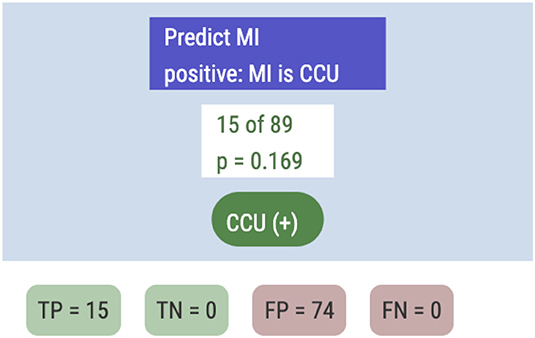
Figure 9. The simplest possible tree.

In this case, TP (the true positive count) is 15 and FP = 74. The ppv will be the base rate, 0.169, and the sensitivity sens will be a perfect 1.0.

Because CCU care is so costly, this plan is impractical in the hospital, and uses none of the diagnostic information. So she drags pain from the data table and drops it onto the white “15 of 89” node. After classifying the nodes, she sees the tree in Figure 10.

FIGURE 10

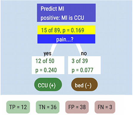
Figure 10. A tree representing the criterion MI and one feature for classification, namely “pain”.

The reader should take a moment to understand the tree display. The “yes” box, for example, tells us that 50 patients experienced chest pain, and 12 of them (24%) got heart attacks. We identified them as being at risk (the green CCU(+) label), a “positive” diagnosis. In the other branch, out of the 39 people we diagnosed as not at risk, three got heart attacks anyway.

Though Dr. Devlin could compute ppv and sens with paper and pencil, she has Arbor “emit” a record of this tree. She sees the table in Figure 11 in CODAP. The system has calculated her measures, showing her that ppv has improved to 0.24, but that sensitivity has declined to 0.8. She then tries the other symptoms—STelev and oneOf—in place of pain, and records the results (Figure 12).

FIGURE 11

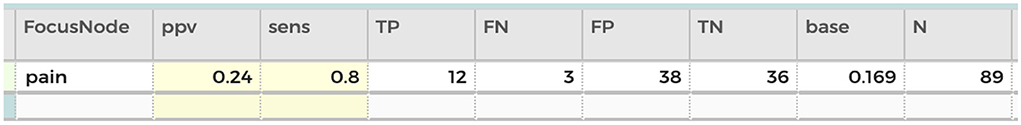
Figure 11. Relevant measures for the feature “pain”.

FIGURE 12

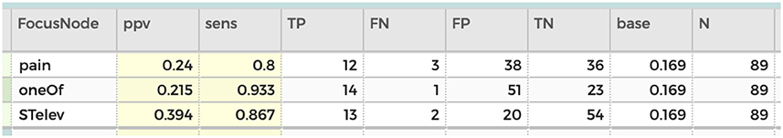
Figure 12. Relevant measures for the three features considered.

Based on this table, Dr. Devlin decides that she likes STelev because it yields so few false positives, saving hospital resources. She decides that she will therefore use ppv as her measure-of-choice and that STelev should be the first cue in the tree.

If she sends everyone with a raised ST segment to the CCU, however, that still leaves two patients who should have gone there (the FNs in the STelev line of the table). So she drops the second-place cue, pain, onto the right-hand branch of the tree (Figure 13).

FIGURE 13

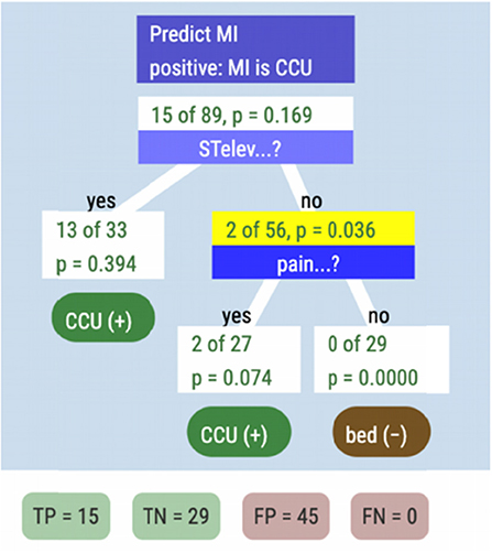
Figure 13. The classification and decision tree with two features.

This captures all of the heart attacks at a cost of more false positives. The ppv of this tree compared to STelev alone has declined from almost 0.4. to 0.25. Perhaps the last cue can help. Dr. Devlin drops oneOf onto the “middle” leaf node, to get our final tree, seen in Figure 14.

FIGURE 14

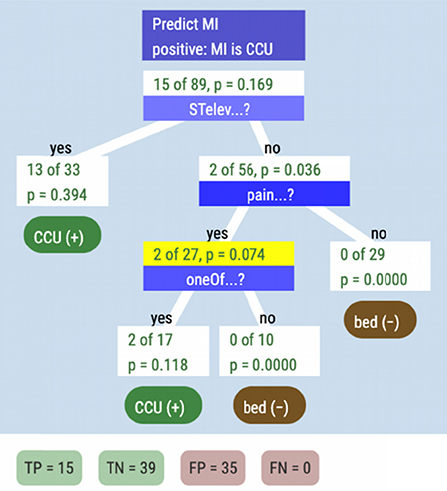
Figure 14. The classification and decision tree based on three cues.

Including one of has improved our ppv to 0.30, and the sensitivity is still 1.0, that is, under this tree, everyone in the Green and Mehr dataset who had a heart attack would have been in the CCU. This is the same tree that appeared in Figure 8.

We might ask whether we could do even better by adding more branches. For example, could we send some of the 20 false positives who had elevated ST segments to regular beds if they had no chest pain? With Arbor, a student (or Dr Devlin) could explore that possibility². But as studies like suggest, that direction can lead to overfitting.

More importantly for our purposes, it leads to additional complication. The frugal tree is easy to implement, especially when you have to act fast: if a patient might have a cardiac event, get an EKG, because the first question, the first node, is about an elevated ST segment. While you're taking the EKG, get the medical history and probe for other symptoms. When the EKG is done, if there's an elevated ST segment, send the patient to the CCU right away. Then, if they have chest pain, check the other 4 symptoms. If they have any of those, send them to the CCU as well. Otherwise, they go to a regular bed for further monitoring at a more leisurely pace. In the meantime, everyone who is most likely to suffer a heart attack has been moved to the place where they can get the best care.

Of course, Dr. Devlin might not upload the data and make the tree herself, though she could. More likely, a best-practices scheme would have been debated and constructed elsewhere using sophisticated AI algorithms and vast datasets.

But let us look in on Dr Devlin, visiting a patient in the CCU, explaining her treatment plan to a frightened old man and his wife. Because Dr Devlin has made decision trees herself, in medical school or in continuing education, she has personal experience with the considerations and tradeoffs that a treatment algorithm inevitably entails. A tree has become part of her personal diagnostic logic rather than a set of steps handed down by some machine. She is better able to implement and accept a tree (or question it with good reason) and better able to explain it: to make a doctor's recommendations more accessible and transparent to her patients.

Comparison of FFT's and other models

The performance of FFT's has been evaluated in several comparisons studies. The first author has collaborated with K. Laskey in an analysis oft he performance of five models, which included two FFT‘s. These five classification methods were tested on eleven data sets taken from the medical and veterinary domains. Most of the data sets were taken from the UC Irvine Machine Learning Repository (Bache and Lichman, 2013). Each data set consisted of a criterion or class variable and five to 22 features. The number of observations ranged from a minimum of 62 to a maximum of 768. The numerical variables were dichotomized by assigning values larger than the median to the “high” ctegory and values less than or equal to the median to the “low” category. The estimation was performed for each model on each data set by taking a random subset of the data as a training sample, dichotomizing numerical variables (if any), applying the fitting method to the training sample, and then classifying each element of the remaining test sample. This process was repeated 1,000 times for each classifier. This process was carried out for training samples of 15, 50, and 90% of the data set. The five classification models are:

• Naïve Bayes

• Logistic regression

• CART (see Breiman et al., 1993)

• Fast and frugal trees with Zig-Zag rule: This method constructs the tree by using positive and negative cue validities. Positive validity is the proportion of cases with a positive outcome among all cases with a positive cue value. Negative validity is the proportion of cases with a negative outcome among all cases with a negative cue value. The Zig-Zag method alternates between “yes” and “no” exits at each level, choosing according to the cue with the greatest positive (for “yes”) or negative (for “no”) validity among the cues not already chosen.

• Fast and frugal trees with MaxVal rule: This method also uses positive and negative cue validities. It begins by ranking the cues according to the higher of each cue's positive or negative validity. It then proceeds according to this ranking, applying the cues in order and exiting in the positive (negative) direction if the positive (negative) validity of the cue is higher. Ties in this process are broken randomly.

Our results are exhibited in Figure 15, below. Performance of the five methods is remarkably similar. Naïve Bayes has the best performance across the board, living up to its reputation as a simple and robust benchmark. The fast and frugal trees are only slightly less accurate than the computationally more expensive naïve Bayes.

FIGURE 15

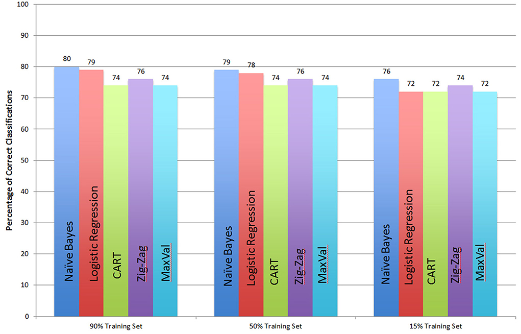
Figure 15. Comparison of 5 classifiers: Naïve Bayes, Logistic Regression, CART, Fast and Frugal tree with a Zig-Zag rule, and with a Max-Val rule.

Concluding remarks

This work has an educational aim. It promotes simple schemes for classification and decision, which are both transparent and easy to grasp. It also promotes dynamical tools which foster the understanding of properties of features, like their sensitivity and predictive value. Transparency is an ideal that decision schemes may have if they are to be part of the communication between patients and doctors.

Data availability statement

Publicly available datasets were analyzed in this study. This data can be found here: Irvine Repository.

Author contributions

RV contributed to the historical introduction on bounded and ecological rationality. TE produced the plugin ARBOR. LM produced the sections on fast-and-frugal trees and the comparisons with other models and wrote large sections of the paper. All authors contributed to the article and approved the submitted version.

Funding

The Ludwigsburg University of Education funds this research.

Conflict of interest

Author TE was employed by Epistemological Engineering.

The remaining authors declare that the research was conducted in the absence of any commercial or financial relationships that could be construed as a potential conflict of interest.

Publisher's note

All claims expressed in this article are solely those of the authors and do not necessarily represent those of their affiliated organizations, or those of the publisher, the editors and the reviewers. Any product that may be evaluated in this article, or claim that may be made by its manufacturer, is not guaranteed or endorsed by the publisher.

Footnotes

1. ^https://www.statnews.com/2022/02/28/sepsis-hospital-algorithms-data-shift/.

2. ^The answer, in this case, is no: out of 10 such patients, 3 had heart attacks.

References

Bache, K., and Lichman, M. (2013). UCI Machine Learning Repository. Irvine, CA: University of California; School of Information and Computer Sciences. Available online at: http://archive.ics.uci.edu/ml

Brase, G. L. (2008). Pictorial representations in statistical reasoning. Appl. Cogn. Psychol. 23, 369–381. doi: 10.1002/acp.1460

PubMed Abstract | CrossRef Full Text | Google Scholar

Breiman, L., Friedman, J. H., Olshen, R. A., and Stone, C. J. (1993). Classification and Regression Trees. New York, NY: Chapman and Hall.

Google Scholar

Casey Ross (2022) AI gone astray: How subtle shifts in patient data send popular algorithms reeling, undermining patient safety. Stat Newsletter. Available online at: https://www.statnews.com/2022/02/28/sepsis-hospital-algorithms-data-shift/.

Conlisk, J. (1996). Why bounded rationality? J Econ Lit. 34, 669–700.

Google Scholar

Daston, L. (1995). Classical Probability in the Enlightenment (Reprint edition). Princeton, N.J.: Princeton University Press.

Google Scholar

Dehaene, S. (1997). The Number Sense - How the Mind Creates Mathematics. New York: NY; Oxford: Oxford University Press.

Google Scholar

Eddy, D. (1982). “Probabilistic reasoning in clinical medicine: problems and opportunities,” in Judgment Under Uncertainty: Heuristics and Biases, eds D. Kahneman, P. Slovic, and A. Tversky (Cambridge: Cambridge University Press), 249–267. doi: 10.1017/CBO9780511809477.019

CrossRef Full Text | Google Scholar

Fischer, J. E., Steiner, F., Zucol, F., Berger, C., Martignon, L., Bossart, W., et al. (2002). Use of simple heuristics to target Macrolide prescription in children with community-acquired pneumonia. Arch. Pediatr. Adolesc. Med. 156, 1005–1008. doi: 10.1001/archpedi.156.10.1005

PubMed Abstract | CrossRef Full Text | Google Scholar

Gage, J., and Spiegelhalter, D. J. (2016). Teaching Probability. Cambridge: Cambridge University Press.

Google Scholar

Garcia-Retamero, R., Okan, Y., and Cokely, E. T. (2012). Using visual aids to improve communication of risks about health: a review. Scientific World Journal, 2012. 562637. doi: 10.1100/2012/562637

PubMed Abstract | CrossRef Full Text | Google Scholar

Gigerenzer, G., and Hoffrage, U. (1995). How to improve Bayesian reasoning without instruction: frequency formats. Psychological Rev. 102, 684–704. doi: 10.1037/0033-295X.102.4.684

PubMed Abstract | CrossRef Full Text | Google Scholar

Gigerenzer, G., and Selten, R. (2002). Bounded Rationality: The Adaptive Toolbox. Cambridge MA: The MIT Press. doi: 10.7551/mitpress/1654.001.0001

CrossRef Full Text | Google Scholar

Gigerenzer, G., Todd, P., and the A. B. C. Group (1999). Simple Heuristics that Make us Smart. Oxford, England: Oxford University Press.

Green, L., and Mehr, D. R. (1997). What alters physicians' decisions to admit to the coronary care unit? J. Family Pract. 45, 219–226.

PubMed Abstract | Google Scholar

Hoffrage, U., Krauss, S., Martignon, L., and Gigerenzer, G. (2015). Natural Frequencies improve Bayesian reasoning in simple and complex tasks. Front. Psychol. 6, 1–14. doi: 10.3389/fpsyg.2015.01473

PubMed Abstract | CrossRef Full Text | Google Scholar

Howson, C., and Urbach, P. (1989). Scientific Reasoning: The Bayesian Approach. La Salle, CA: Open Court Publishing.

Google Scholar

Howson, C., and Urbach, P. (2006). Scientific Reasoning: the Bayesian Approach.

Google Scholar

Jenny, M. A., Pachur, T., Williams, S. L., Becker, E., and Margraf, J. (2013). Simple rules for detecting depression. J. Appl. Res. Mem. Cogn. 2, 149–157. doi: 10.1037/h0101797

CrossRef Full Text | Google Scholar

Kahneman, D., Slovic, P., and Tversky, A. (1982). Judgment Under Uncertainty: Heuristics and Biases. Cambridge: Cambridge University Press. doi: 10.1017/CBO9780511809477

PubMed Abstract | CrossRef Full Text | Google Scholar

Katsikopoulos, K., Simşek, Ö., Buckmann, M., and Gigerenzer, G. Feb (2021) Classification in the Wild: The Science Art of Transparent Decision Making. Boston: MIT Press. doi: 10.7551/mitpress/11790.001.0001

CrossRef Full Text | Google Scholar

Kroes, P., Franssen, M., and Bucciarelli, L. (2009). “Rationality in Design” in Philosophy of Technology and Engineering Sciences. Amsterdam: Elsevier. doi: 10.1016/B978-0-444-51667-1.50025-2

CrossRef Full Text | Google Scholar

Kurz-Milcke, E., Gigerenzer, G., and Martignon, L. (2008). Transparency in risk communication: graphical and analog tools. Ann N Y Acad Sci. 1128, 18–28. doi: 10.1196/annals.1399.004

PubMed Abstract | CrossRef Full Text | Google Scholar

Laplace, P. S. (1812). Théorie analytique des probabilités. Paris, Ve. Courcier. Available online at: http://archive.org/details/thorieanalytiqu01laplgoog

Google Scholar

Lötsch, J., Kringel, D., and Ultsch, A. (2022). Explainable artificial intelligence (XAI) in biomedicine. Making AI decisions trustworthy for physicians and patients. Biomedinformatics. 2, 1–17. doi: 10.3390/biomedinformatics2010001

CrossRef Full Text | Google Scholar

Luan, S., Schooler, L. J., and Gigerenzer, G. (2011). A signal detection analysis of fast-and-frugal trees. Psychol. Rev. 118, 316–338. doi: 10.1037/a0022684

PubMed Abstract | CrossRef Full Text | Google Scholar

Martignon, L., and Laskey, K. (2019). Statistical literacy for classification under risk: An educational perspective. AStA Wirtschafts- Und Sozialstatistisches Archiv. 13, 269–278. doi: 10.1007/s11943-019-00259-3

CrossRef Full Text | Google Scholar

Martignon, L., Vitouch, O., Takezawa, M., and Forster, M. (2003). “Naïve and yet enlightened: From natural frequencies to fast and frugal decision trees,” in Thinking: Psychological Perspectives on Reasoning, Judgment, and Decision Making, eds D. Hardman and L. Macchi (Chichester: John Wiley and Sons), 189–211.

Google Scholar

Massaro, D. (1998). Perceiving Talking Faces. Cambridge, MA: MIT Press.

Google Scholar

Simon, H. (1978). Rational Decision Making in Business Organizations. Noble Prize Lectures.

Google Scholar

Simon, H. (1983). Reasons in Human Affairs. Stanford University Press.

Google Scholar

Simon, H. (2001). “Rationality in Society,” in International Encyclopedia of the Social and Behavioral Sciences (Amsterdam: Elsevier). doi: 10.1016/B0-08-043076-7/01953-7

CrossRef Full Text

Viale, R. (2021a). Handbook of Bounded Rationality. London: Routledge. doi: 10.4324/9781315658353

CrossRef Full Text | Google Scholar

Viale, R. (2021b). “Psychopathological Irrationality and Bounded Rationality” in Routledge Handbook on Bounded Rationality, ed R. Viale (London: Routledge).

Google Scholar

Viale, R. (2021c). The epistemic uncertainty of Covid-19: failures and successes of heuristics in clinical decision making. Commun. Earth Environ. 20, 149–154. doi: 10.1007/s11299-020-00262-0

CrossRef Full Text | Google Scholar

Woike, J. K., Hoffrage, U., and Martignon, L. (2017). Integrating and testing natural frequencies, naïve Bayes, and fast-and-frugal trees. Decision. 4, 234–260. doi: 10.1037/dec0000086

CrossRef Full Text | Google Scholar