A low-cost close-range photogrammetric surface scanner

1 Introduction

Close-range photogrammetry is a technique used to create accurate three-dimensional (3D) models of surfaces from relatively short distances. The motivation for the close range is the detailed reconstruction of the structure and appearance of these surfaces. Close-range photogrammetry finds application in the micrometer-range reconstruction of structures in industrial (Luhmann, 2010; Rodríguez-Martín and Rodríguez-Gonzalvez, 2018; Rodríguez-Martín and Rodríiguez-Gonzálvez, 2019), biological (Fau et al., 2016), archaeological (Gajski et al., 2016; Marziali and Dionisio, 2017), anthropological (Hassett and Lewis-Bale, 2017), and cultural (Fernández-Lozano et al., 2017; Inzerillo, 2017) applications; see Lussu and Marini (2020) for a comprehensive review of close-range photogrammetry applications.

However, when compared to other surface scanning methods, close-range photogrammetry is a cost-effective choice; it often requires specialized hardware that is less expensive but still costly. Moreover, several difficulties hinder its application. Practical difficulties relate to the numerous images required to cover a given surface area, the tedious process of setting up and calibrating, and the avoidance of shadows and reflections, which affect the quality and accuracy of results. Imaging difficulties relate to the close-range imaging of surfaces, which has a very short depth of field, severe lens distortion, and limited field of view (FoV). Algorithmic difficulties relate to the accumulation of geometric errors when using large numbers of images.

To alleviate practical difficulties an apparatus is proposed that uses computer numerical control (CNC) to move the camera to designated locations and automatically acquire images with the same illumination conditions at each pose. This motorization undertakes the burden for the operator, making it robust against human errors. Moreover, it records the (nominal) camera location and associates it with the acquired image. This information is exploited for the proposed reconstruction method.

To retain a low cost, an off-the-self consumer-grade camera and open printable CNC parts are utilized. Specifically, this work reuses the hardware of the contactless flatbed photogrammetric scanner used by Zabulis et al. (2021), which is composed of off-the-shelf and printable components, provides 2D image mosaics of surfaces in the micrometer range, and costs less than US$1,000.

To address algorithmic difficulties, an image acquisition approach and a reconstruction method are proposed, designed to reduce the reconstruction complexity and errors.

The utilized CNC device is shown in Figure 1 (left), with its three axes of motion superimposed; red, green, and blue correspond to the xx′-, yy′-, and zz′-axes, respectively. This camera faces the target surface perpendicularly. The device is used to methodically acquire images across the surface region (xx′- and yy′-axes) and at different distances, or elevations, (zz′-axis) from the surface. In Figure 1 (right), the characteristic elements of the proposed image acquisition are illustrated. Shown is the camera at viewpoints a, b, and c. Viewpoints a and b are at the same elevation and exhibit lateral overlap. Viewpoint c is at a higher elevation and images a surface region that includes the regions imaged from viewpoints a and b; this type of overlap across layers is referred to as medial overlap.

Figure 1

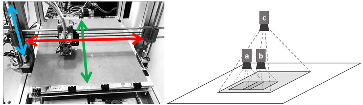
Figure 1. The computer numerical control device (left) and illustration of image acquisition across distances (right).

This work brings the following novel characteristics: It uses auxiliary images from multiple distances to create more accurate surface reconstructions. It furthermore uses tracking of the features across images at multiple distances to enhance accuracy. Furthermore, it uses a Cartesian motorized platform for image acquisition (as opposed to the conventional turntable configuration), which enables the scanning of wider areas. In addition, it provides higher resolution than other methods reported in the literature. Last but not least, it can be implemented in a very cost-efficient manner, in terms of hardware, compared to other approaches. To the best of our knowledge, it is the first method that utilizes images at multiple distances to improve the accuracy of the surface reconstruction result.

The imaging resolution for surface scanning is denoted as measured by the number of pixels, or points, per unit area in metric units, that is, p/mm². To ease the comparison with off-the-shelf scanners, the equivalent of dots per inch, that is, points per inch (ppi), is also used. The ppi is a 1D metric that denotes the resolution of points across a line, and thus, a resolution of 100ppi means that in the scanned image, 100 × 100 = 10 Kp would be devoted for a surface area of 1 in × 1 in = 1 in². It is equivalent to saying that the scanned image has a resolution of 10 Kp/in² (number of points/per square inch).

2 Related work

As reviewed in the following, the vast majority of close-range photogrammetric methods use a turntable to acquire images around the scanned object. Although this configuration is suitable for 3D objects, it is constraining for surfaces in terms of the spatial extent that can be reconstructed. The reason is that as the size of the object becomes larger, the central locations of the object occur farther away from the camera and are imaged in lower resolution. Thus, when using a turntable, the target object is required to be imaged from multiple angles that comprise a hypothetical hemisphere above the scanned target. This requirement adds to the constraints of the imaging apparatus, making it cumbersome and increasing its cost. The conditions required for surface scanning have been explored in more depth in aerial, far-range photogrammetry, for the digitization of Earth surfaces. In these cases, images are acquired from locations that form a Cartesian grid. The reconstruction is aided by GPS coordinates and gyroscope measurements available during image acquisition, which aid the accuracy of extrinsic camera parameter estimation.

In the remainder of this section, we first review the cost and applicability benefits of photogrammetry compared to other modalities for highly detailed surface scanning. Then close-range photogrammetric methods are reviewed in terms of the hardware they employ to motorise camera motion, the optics they use, and the illumination that they adopt. Next, the methods in the literature are reviewed as to the data acquisition specifications that they offer and the reconstruction methods they employ. Afterward, the ways that the scale factor is estimated for close-range photogrammetric methods are outlined. Next, recent variants and uses of close-range photogrammetry are reviewed. Finally, the contributions of this work are outlined.

2.1 Comparison with other modalities for surface scanning

Besides photogrammetry, other modalities for surface scanning in large detail are the following: Computed tomography (CT) uses X-rays to provide volumetric scans of objects and their surfaces and has been used for the digitisation of small objects (Illerhaus et al., 2002). Magnetic resonance (MR) tomography has been also used for detailed volumetric scans of small objects (Semendeferi et al., 1997). Laser scanning uses the time-of-flight principle to measure distances and reconstruct surfaces. Structured light scanners project light patterns onto surfaces, capture the deformed patterns using a camera, and from these deformations, estimate surface structure. Other close-range photogrammetric approaches exhibit significant constraints as to the scanning area and hardware requirements and are reviewed in Section 2.

Although highly accurate, tomographic methods (CT, MR) exhibit severe costs and can be applied only in specialized laboratories. Moreover, they provide volumetric and accurate structure reconstruction but do not reconstruct surface appearance (texture). Laser scanning and structured light scanning capture surface appearance, are marginally less accurate, and are more cost-efficient because they require less equipment. Photogrammetry is even more affordable and widely available, as it relies on standard cameras only. Moreover, photogrammetry excels in capturing the appearance of surfaces because it images surfaces without the effects of active illumination. Photogrammetry produces high-resolution and highly detailed textured models that accurately represent visual appearance. Compared to laser and structured light methods, photogrammetry can be less accurate but is passive in that it does require the projection of energy in the form of radiation (e.g., light, X-rays, etc.) upon the scanned surface. This is important for light-sensitive materials, encountered in historical, archaeological, biological, and cultural contexts.

2.2 Close-range photogrammetry

2.2.1 Motorisation

The motorization of camera movement has been used in photogrammetric reconstruction to alleviate user effort and acquire images at numerous prescribed viewpoints. The main strategies of motion are either circular around the target, using a turntable, or in a Cartesian lattice of viewpoints (Lavecchia et al., 2017). Cartesian approaches exhibit the advantages of being unconstrained of the turntable size and that the camera can be moved arbitrarily close to the scanning target. This work follows the latter approach to scan wider surface areas and avoid the occurrence of shadows and illumination artifacts. The most relevant motorized scanning apparatus to this work is presented by Gallo et al. (2014), which also uses CNC to move the camera.

2.2.2 Optics

In the millimeter and submillimetre range, zoom and microscopic, or “tube,” lenses have been used (González et al., 2015; Percoco and Salmerón, 2015; Lavecchia et al., 2017), employing tedious calibration procedures and relatively inaccurate results (Shortis et al., 2006). Instead, macro lenses are more widely used in the photogrammetric reconstruction of such small structures (Galantucci et al., 2018). Both lens types exhibit a very limited depth of field.

To compensate for the limited depth of field, focus stacking (Davies, 2012), an image-processing technique for the enhancement of the depth of field, is widely used in macro photography and, subsequently, in close-range photogrammetry (Galantucci et al., 2013; Mathys and Brecko, 2018). Focused-stacking techniques capture a scene in a series of images, each focused at a gradually different depth, and combine them in a composite image with an extended depth of field. Focus stacking is often embedded in the hardware of consumer-grade macro cameras.

2.2.3 Lighting

Lighting configuration is essential in photogrammetry. The main goal is to prevent shadows and highlights, both of which hinder the establishment of correspondences. In the close-range photogrammetry of objects and surfaces, set-ups have been used that insulate the target object from environmental illumination and use a specific light source in conjunction with illumination diffusers to prevent the formation of shadows. More recently, ring-shaped light sources around the lens are often employed to provide (approximately) even and shadow-free illumination. In close-range photogrammetry, the latter approach is adopted, and some systems use light sources that move along with the camera (Galantucci et al., 2015; Percoco et al., 2017a,b).

2.2.4 Structured lighting

Purposefully designed illumination is used by some photogrammetric methods to facilitate the establishment of stereo correspondences. This technique is known as “active illumination,” “active photogrammetry,” or “structured light” (Percoco et al., 2017a; Sims-Waterhouse et al., 2017a,b). Pertinent methods project patterns of light to artificially create reference points on surfaces that can be matched across images. The main disadvantage is that the projected light either alters the visual appearance of the reconstructed surfaces or is in the infrared domain and detected by an additional camera. In both cases, additional hardware and/or image acquisitions are needed to obtain photorealistic reconstructions.

2.2.5 Scanning area and resolution

Reported apparatuses for close-range photogrammetry vary depending on imaging specifications.

Studies that report scanning areas fall in the range of approximately [0.14, 158.7] cm². Specifically, the maximum area reported from these studies is (approximately) as follows: 0.14cm² (González et al., 2015), 10cm² (Sims-Waterhouse et al., 2017b), 15cm² (Percoco et al., 2017a), 22.5cm² (Marziali and Dionisio, 2017), 25cm² (Lavecchia et al., 2018), 32cm² (Gallo et al., 2014), 40cm² (Galantucci et al., 2015), 57.6cm² (Galantucci et al., 2016), 60 cm² (Gajski et al., 2016), 91.5m² (Percoco and Salmerón, 2015), 93.4cm² (González et al., 2015), and 158.7cm² (Galantucci et al., 2016). Out of these studies, only González et al. (2015) report the achieved resolution, which is 3, 745p/mm².

Studies that report the number of images and pixels processed fall in the range of [9.6, 3, 590.0] Mp. The data load is calculated as the number of utilized images times the resolution of each image. Specifically, the maximum number of pixels reported from these studies is (approximately), in Mp, as follows: 16 × 0.6 = 9.6 (Percoco and Salmerón, 2015), 7 × 10.1 = 70.7 (Percoco et al., 2017b), 12 × 10.1 = 121.2 (Lavecchia et al., 2018), 30 × 24 = 720.0 (Sims-Waterhouse et al., 2017a), 72 × 12.3 = 885.6 (Gallo et al., 2014), 40 × 36.3 = 1, 452.0 (Marziali and Dionisio, 2017), 245 × 10.2 = 2, 499.0 (Fau et al., 2016), and 359 × 10 = 3, 590.0 (Galantucci et al., 2015).

2.2.6 Reconstruction

Some of the reviewed approaches perform partial reconstructions, which result in individual point clouds, and then merge them using point-cloud registration methods. These methods are mainly based on the iterative closest point algorithm (Besl and McKay, 1992; Yang and Medioni, 1992), either implemented by the authors or provided by software utilities, such as CloudCompare and MeshLab. The disadvantages of merging partial reconstructions are the error of the registration algorithm and the duplication of surface points that are reconstructed by more than one view. These disadvantages impact the accuracy and efficacy of the reconstruction result, respectively.

2.2.7 Scale factor estimation

Several methods have been proposed for generating metric reconstructions. One way is to place markers at known distances so that when they are reconstructed, they yield estimates of the absolute scale. However, this method is prone to the localization accuracy of said markers. An improvement to this approach comes from Percoco et al. (2017b), who used the ratio of the reconstructed objects over their actual size, which is manually measured. However, it requires the careful selection of the reference points to estimate the size of the object both in the real and the reconstructed objects and is, thus, prone to human error. This can be a difficult task for free-form artworks as they may not exhibit well-defined reference points, that is, as opposed to industrially manufactured objects. Therefore, the accuracy of this approach is dependent on the accuracy of manual measurements of the actual object and its reconstruction.

Another way to achieve metric reconstruction is to include objects of known size in the reconstructed scene, such as printed 2D or 3D markers (Galantucci et al., 2015; Percoco et al., 2017b; Lavecchia et al., 2018). This method does not involve human interaction and is not related to the structure of the reconstructed objects. The main disadvantage of this approach is the production of these markers, as printing markers at a micrometer scale is not achievable by off-the-shelf 2D or 3D printers.

One way to estimate the scale factor is based solely on the reprojection error of the correspondences of a stereo pair (Lourakis and Zabulis, 2013). This approach is independent of the shape of the target object and does not require human interaction. However, this approach is formulated for a stereo pair and not for a single camera.

2.3 Recent adaptations and variants of close-range photogrammetry

The theory of photogrammetry has been studied in depth over the last three decades, with most of its aspects being well-covered by a staggering number of studies. As a result, several off-the-shelf products nowadays exist and are being used in several applications, with Agisoft, Pix4D, 3DF Zephyr, and PhotoCatch reported most widely. More recent works in the field of close-range photogrammetry focus on image acquisition protocols, complementary steps, parameter optimization, and the utilization of domain-specific knowledge. In the following, some recent and characteristic examples are reviewed.

A recent algorithmic improvement relevant to the application of close-range photogrammetry can be found in Eldefrawy et al. (2022), where an independent preprocessing step is introduced in the conventional structure-from-motion (SfM) pipeline for detecting and tracking of multiple objects in the scene into isolated subscenes. The approach uses a turntable and is not relevant to surface scanning, which is the focus of this work.

The approach detailed by Paixão et al. (2022) uses conventional photogrammetry to reconstruct a rock surface. It uses a turntable to collect images from multiple views and two elevation levels. The method is reported to handle up to 72 images and achieve a maximum resolution of 22.5 p/mm². It employs manual effort in cleaning noise from the reconstruction using the MeshLab 3D editor. Lauria et al. (2022) used a turntable and a 30-cm imaging distance to create photogrammetric reconstructions of human crania. The proposed approach elaborates on the imaging conditions to provide a guide of the photo acquisition protocol and the photogrammetric workflow while using conventional SfM single-camera photogrammetry.

Close-range photogrammetry is employed in the detailed analysis of geological structures. Conventional photogrammetry was used by Jiang et al. (2022) to reconstruct soil surfaces and assess rill erosion. Harbowo et al. (2022) used close-range (1-cm) photogrammetry to reconstruct meteorite rock structures. Fang et al. (2023) used a turntable and conventional photogrammetry are used to measure the size and shape of small (≈5-mm) rock particles.

An application domain of close-range photogrammetry regards dental structures, which often exhibit shiny reflectance properties. The method used by Furtner and Brophy (2023) reconstructs small and shiny dental structures, using the Agisoft photogrammetry suite; in this case, specular reflections and shadows are manually removed using post-processing of the acquired images in Adobe Photoshop Elements. The approach Yang et al. (2023) used included a PhotoCatch photogrammetric application for mobile phones to create a 3D reconstruction of dental structures; specular reflections were blocked using two custom light-blocking filters and two circular polarisers. Scaggion et al. (2022) used the 3DF Zephyr photogrammetric suite to reconstruct individual teeth; in this case, the structures were highly diagenized and were not shiny. Kurniawan et al. (2023) used conventional SfM-based photogrammetry for the forensic evaluation of human bite marks in matte wax surfaces. Dealing with shiny surfaces was also considered in the approach used by Petruccioli et al. (2022), but they utillized an application of matting spray while using conventional turntable photogrammetry in combination with highly controlled illumination.

Guidi et al. (2020) investigated the relation between the amount of image overlap in the acquisition of photogrammetric data and reconstruction accuracy, leading to the conclusion that a larger overlap is required in close-range photogrammetry (>80%) than that in conventional photogrammetry (40–60%). The experiments performed in this work required a turntable, manual intervention, and incorporating imaging distances of 20 cm. The results of this study coincide with those of the proposed approach in which a large overlap is employed.

Context domain knowledge was employed by Dong et al. (2021), which uses the Pix4D photogrammetric suite to reconstruct tree structures; the approach is characterized as close range compared to aerial photogrammetry, although the imaging distance is several meters. The method further uses domain-specific knowledge (tree structure) to optimize the reconstruction of tree trunks and is not a generic photogrammetric method. Lösler et al. (2022) used conventional photogrammetry and bundle adjustment to estimate the pose of a telescope by reconstructing markers at known locations.

2.4 This work

This work puts forward a photogrammetric approach powered by a motorized apparatus and implemented by a modest computer and a conventional CNC device. The photogrammetric approach is characterized by two novel characteristics. First, a tailored image acquisition is implemented using said apparatus that acquires an image of the target surface at multiple elevations (distances). Second, key point features are tracked across multiple views and at multiple distances instead of only being corresponded in neighboring images.

The aforementioned algorithmic characteristics are deemed necessary to increase the scanned area as well as reconstruct the surface with accuracy and precision. The main problem that they solve stems from the large number of images required to cover a relatively wide area in high resolution. When the number of images grows large, that is, tens of thousands, problems that are less pronounced when using fewer images become quite intense. Specifically, when the number of images is large, even minute camera pose estimation errors accumulate in significantly inaccurate reconstruction results.

The proposed approach combines two elements that increase its robustness against hardware and camera motion estimation errors and, thereby, obtain more accurate reconstructions:

1. Auxiliary images are acquired at larger distances (>α) than the distance at which the surface is photographed. These images are fewer in number than the images acquired at distance α. The auxiliary images are not used in the texturing of the reconstructed surface. They are used to ensure that the mosaicing of partial scans into a larger one is consistent with the overall structure of the surface as overviewed from larger distances.

2. Tracking of features across images. Usually, photogrammetric methods find and reconstruct correspondences only in neighboring views. From these, stereo-correspondent partial 3D reconstructions are obtained, which are, in turn, registered into a composite reconstruction. This work tracks features that belong to the same physical point across multiple views and distances. The constraints obtained from this tracking are utilized to reduce spurious feature correspondences and, thereby, increase reconstruction accuracy.

To the best of our knowledge, this work improves state of the art in the following ways: First, a qualitative comparison with the state of the art indicates that conventional photogrammetry exhibits distortions in the conditions of interest and that are the conditions we are testing. Second, the proposed approach exhibits a significantly lower cost and ease of use compared to close-range photogrammetry methods found in the literature, which require high-end cameras and highly controlled illumination. The proposed approach deals with shiny surfaces without needing additional optical filters and without requiring setting up the illumination conditions. In addition, the proposed approach is fully automatic without the need for human intervention, which is the case in many of the studies reported in the literature. Third, due to the Cartesian approach to image acquisition, the proposed approach can reconstruct wider areas than works reported in the literature.

3 Method

The proposed method consists of the following steps.

3.1 Camera calibration

Photogrammetric reconstruction requires estimates of intrinsic and extrinsic camera parameters. Intrinsic parameters include the resolution and optical properties of the visual sensor. Extrinsic parameters include its position and orientation in space and represent the estimation of camera motion relative to the target surface.

3.1.1 Intrinsic parameters

The camera is calibrated to estimate its intrinsic parameters and its lens distortion, using the methods used by Heikkila and Silven (1997) and Zhang (1999). The intrinsic parameters represent the location of the optical center, the skew of the optical axis, and the focal length of the camera. The FoV of the camera is also derived from these parameters. In addition, lens distortion is also estimated in this step. The aforementioned parameters are independent of the camera location and, thus, are estimated once before mounting the camera.

3.1.2 Extrinsic parameters

Extrinsic parameters represent the orientation and the location of the camera, as a rotation and translation of the camera concerning some world coordinate system.

An initial estimate of extrinsic camera parameters is provided by the CNC device and specifically from the readings of the stepper motor controllers that move the camera. The area of the scan table and the elevation range are measured to estimate the motor step length per dimension, given that these motors produce equal motion steps. The number of horizontal and vertical steps are denoted as n_x and n_y, while the length of the horizontal and vertical steps s_x and s_y, respectively.

Steps s_x and s_y, are defined in metric units. Thereby, the obtained initial estimate of the extrinsic parameters is also in metric units. This initial estimate of camera locations is refined in Section 3.5.2.

3.2 Image acquisition

Although the CNC apparatus acquires all images in one pass, the acquired images are conceptually classified in layers of elevation from the scanned surface.

Within each layer, viewpoints are organized in a lattice, as illustrated in the example of Figure 2 (left). In the example, n_x = 4 and n_y = 5. Solid lines mark the surface regions imaged by the camera. Dots mark camera center locations. The horizontal and vertical distances between camera centers are denoted as s_x and s_y, respectively. Transparent regions indicate the lateral overlap between neighboring images of the same layer. The FoV of the camera and the required amounts of lateral and medial overlaps determine the values of s_x and s_y and the distances between layers. The same proportion of lateral overlap is used for both horizontal and vertical dimensions, τ_o.

Figure 2

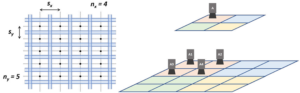
Figure 2. Illustrations of the computer numerical computer motion parameterization for one layer (left) and image acquisition across layers (right).

Across elevation layers, viewpoint locations are configured hierarchically, so that the images from “parent” viewpoints at higher layers medially overlap with “child” viewpoints at lower layers by a factor of τ_m. This is illustrated in Figure 2 (right), where viewpoint A overviews the area imaged by viewpoints A1, A2, A3, and A4. When τ_m = 25%, as in the example, the hierarchical structure has the form of a quad-tree. The top layer, indicating the upper end of this frustum, is user-determined.

The camera centers are pre-computed and saved in a file, which is called the “scan plan”. These locations are then converted to scanner coordinates, and a corresponding segment of G-code¹ is generated. This code is transmitted to the CNC, and images are acquired using the software interface from Zabulis et al. (2021). The image file names are associated with the camera locations in the scan plan. To reduce the scanning time and mechanical drift, each layer is scanned in boustrophedon order.

3.3 Feature detection and matching

Key point features with content descriptions are detected in all images. In the implementation, scale-invariant feature transform (Lowe, 2004) features are employed, but any other type of key point features can be used. Matching takes place between all pairs of laterally or medially neighboring images. These pairs are found from the scan plan and denoted as (I_i, I_j) for neighboring images I₁ and I_j.

3.3.1 Cascade hashing

To accelerate feature matching, the cascade hashing method used by Cheng et al. (2014) is employed. Cascade hashing significantly reduces the feature search space by discarding non-matching features early and at a low cost. The method creates multiple hash tables, each capturing a different aspect of the feature descriptor. A global hash table captures high-level information about the descriptor. This table helps quickly eliminate many non-matching candidates. At lower levels, more specific hash tables capture increasingly detailed information about the descriptors. By descending through the levels, the number of potential candidates decreases, and the matching becomes more precise.

3.3.2 Fundamental matrices

The fundamental matrix F is defined for a pair of images and defines the geometric constraints that exist between points in the first image and their corresponding epipolar lines in the other image (Hartley and Zisserman, 2003) and vice versa for its inverse matrix. In this step, the fundamental matrices, F_{i, j}, for all pairs of laterally and medially neighboring images are computed, where F_{i, j} denotes the fundamental matrix for image pair (I_i, I_j).

Matrices F_{i, j} are estimated from the available correspondences between pairs of neighboring images (I_i, I_j). Initially, spurious correspondences (“outliers”) are discarded using random sample consensus (RANSAC; Fischler and Bolles, 1981). The remaining “inlier” correspondences are used to estimate F_{i, j}, using least squares fitting.

The estimated matrices F_{i, j} are stored and are used in the next steps to implement “epipolar constraints” and discard spurious correspondences. The epipolar constraint is implemented as follows: Let homogeneous coordinates p_i and p_j represent the 2D locations where the same physical point appears in I_i and I_j, respectively. The epipolar constraint is expressed as ${\text{p}}_j^T·F_{i,j}·{\text{p}}_i<{\tau }_c$, where threshold τ_c is a distance (scalar). This distance expresses how well the correspondence complies with epipolar constraint and is the distance of the projection of p_i to I_j (using F) from its epipolar line in I_j. The smaller the τ_c the better the compliance and the more reliable the correspondence. Threshold τ_c is defined as an input parameter relevant to imaging factors such as image resolution and imaging distance.

It ought to be noted that, theoretically, F could be calculated for each image pair using the intrinsic parameters of the camera and the relative poses of camera pairs from the scan plan instead of the aforementioned procedure. In practice, however, it was found that the small mechanical inaccuracies of the CNC lead to erroneous F estimates. The resulting error is large enough to render the estimated F overly inaccurate for outlier elimination making the previously mentioned task necessary.

3.3.3 Left-to-right check

To filter erroneous correspondences a symmetric, or left-to-right check (Fua, 1993) is employed. The goal of this check is to ensure that correspondences are consistent for both images, which helps filter out incorrect matches. For each correspondence pair, the epipolar constraint is calculated two times: once for image pair (I_i, I_j) and once for image pair (I_j, I_i). In practice, the equations for each part of the check are ${\text{p}}_j^T·F_{i,j}·{\text{p}}_i<{\tau }_c$ and ${\text{p}}_i^T·F_{i,j}^T·{\text{p}}_j<{\tau }_c$. If both constraints are not satisfied, then the correspondence is discarded.

In other words, to establish a feature correspondence, it is required that the same key point feature pair is found both when features of I_i are matched against I_j and vice versa. Conventionally, to avoid doubling the computational cost, when establishing matches in one direction, key point similarities could be recorded and utilized when scanning in the opposite order. Unfortunately, our graphics processing unit (GPU) random-access memory (RAM) is not sufficient to record this information, for large targets. Thus, {I_i, I_j} and {I_j, I_i} are treated independently, and the doubling of computational cost is not avoided. If a GPU with larger memory were available, the aforementioned method could be employed to halve the computational cost of this task.

3.4 Feature tracking

Despite the action of the check-in (Section 3.3.3), the correspondences found at this stage still contain errors. This step detects and further reduces spurious correspondences, aiming at a more accurate reconstruction result.

Features are tracked across images, as follows. Let N key point features that corresponded in N images. Let u_i, i∈[1, N] their locations in these images. Points u_i comprise a “feature track.” If the track contains spurious correspondences, then some of u_i shall not image the same physical point. No specific order is imposed on the elements of the feature track. Feature tracks are not only constrained in laterally neighboring images but are also established using correspondences across layers as well. This is central to achieving overall consistency in surface reconstruction. The reason is that the spatial arrangement of features in images of greater distance to the surface constrains the potential correspondences in images at closer distances.

Each track is evaluated as follows: Let $F_{1,N}^{\prime }=F_{1,2}·F_{2,3}·\dots F_{N-1,N}$ a composite fundamental matrix of the pair of images that contain u₁ and u_N, that is, the first and last elements of the track. Images I₁ and I_N may not be direct neighbors. Even if they are, still $F_{1,N}^{\prime }$ is used instead of the F_{1, N} computed in Section 3.3.2. The reason is to involve all correspondences referenced in the feature track and, in this way, detect whether any of them is spurious.

Using $F_{1,N}^{\prime }$, image location u₁ is projected to image I_N, which contains location u_N. The location of this projection is ${\text{u}}_p=F_{1,N}^{\prime }·{\text{u}}_1$, and the distance of these two points is δ = |u_p−u_N|. If the correspondences in the feature track are correct, then these points should approximately coincide as only calibration inaccuracy should account for δ. However, if the track contains erroneous correspondences, then the two locations are expected to be grossly inconsistent and δ to be greater than the distance threshold τ_p. Thus, if δ>τ_p, then the feature track and all of its correspondences are discarded.

The memory requirements for the succeeding tasks depend on the number of tracked features found. Depending on the number of input images the requirements for memory capacity may be large. It is possible to reduce the memory capacity requirements at this stage by discarding some of the feature tracks. If this is required, then it is recommended to discard the tracks with the fewest features. The reason is that they carry less information and are, typically, much larger in number.

3.5 Reconstruction

Using the obtained correspondences, the scanned surface is reconstructed as a textured mesh of triangles.

3.5.1 Initialization

Using the obtained feature tracks as a connectivity relation, a connected-component labeling of the input images is performed. After this operation, the largest connected component is selected. The rest of the images, which belong to smaller components, are discarded. The discarded components correspond to groups of images that are not linked, through fundamental matrices, to the rest. As such, they cannot contribute to the main reconstruction. They are, thus, discarded to reduce the memory capacity requirements.

The reconstruction method requires an image pair, (i′, j′), as the basis for the surface reconstruction. This pair is selected to exhibit a wide baseline to reduce reconstruction uncertainty and error (Csurka et al., 1997). The reason is that wider baselines result in more separation between the optical rays, reducing ambiguity in the 3D reconstruction. At the same time, the reliability of this pair depends on the number of feature correspondences existing in this pair. Thus, the initial pair is selected as the product of baseline with the number of correspondences, or $(i^{\prime },j^{\prime })=arg\underset{i,j}{max}(b_{i,j}·k_{i,j})$, where b_{i, j} is the baseline of pair (i, j) and k_{i, j} is the number of feature correspondences between I_i and I_j.

3.5.2 Sparse reconstruction

A sparse reconstruction is first performed, using the camera poses in the scan plan of the correspondences obtained from Section 3.2. The purpose of this reconstruction is to refine these pose estimates. Open Multiple View Geometry (Moulon et al., 2016) is utilized to obtain a sparse point cloud, which includes implementations of the incremental structure-from-motion pipeline (Moulon et al., 2013) and AC-RANSAC (Espuny et al., 2014).

The purpose of the far-range images is encountered in this step. The large number of images, that is, tens of thousands, required to photogrammetrically cover wide surfaces in large detail, pose accuracy problems that are not intensely pronounced when reconstruction involves a few hundred images. In the context of thousands of images, even small registration errors may accumulate, leading to globally inconsistent surface structures. As correspondences include pairs of points across layers, the reconstruction process is guided to produce a structure that is consistent with far-range views. In the experiments (Section 4), it is observed that these additional constraints reduce global distortion errors in the final result.

A bundle adjustment, used by Lourakis and Argyros (2009), is then performed in the end. This operation is adapted to optimize only the lens distortion and the extrinsic parameters for each image. The reason is to ease the convergence of the bundle adjustment optimization, as the intrinsic camera parameters have been accurately estimated in Section 3.1.

The method is formulated in Algorithm 1.

Algorithm 1

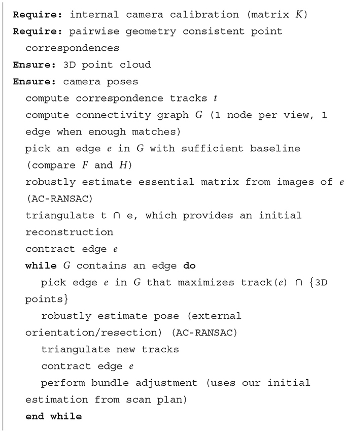
Algorithm 1. Incremental structure from motion.

Finally, the scale factor is estimated at this step. In contrast to the methods in Section 2.2.7, this work estimates scale factor using the extrinsic parameters of the camera. This accuracy is relatively high because they are founded on the accurate motorization of CNC devices. The initial estimates of camera locations obtained from the scan plan are already in metric units and, thus, are the refined ones.

3.5.3 Dense and textured reconstruction

A mesh of triangles is computed based on the obtained sparse point cloud from Section 3.5.2. In the implementation, the OpenMVS (Cernea, 2008) library is utilized.

The “Z-buffering technique” (Catmull, 1974) is employed to obtain depth maps, D_i. These maps are images that have the same dimensions as I_i, imaging the scene from the same viewpoint as I_i and with the same intrinsic parameters. In D_i(u), each depth map stores the distance of the surface point imaged at I_i(u) from the optical center that I_i was acquired. Given the camera extrinsics, the pixels of the depth map are converted into a point cloud in world coordinates. In this way, depth maps D_i are aggregated in a dense point cloud, using the procedure from Barnes et al. (2009). Following Jancosek and Pajdla (2014), a global mesh surface that best explains the dense point cloud is generated. Afterwards, this mesh is refined via the variational method used by Hiep et al. (2011).

Next, index maps T_i are computed, which store at each pixel the identification of the mesh triangle, imaged at that pixel; that is, in T_i(u), the identification of the triangle that is imaged at u is encoded. Using maps D_i and T_i, texturing the mesh considers the visibility of the triangle in each I_i. When a triangle is imaged in multiple views, then several choices can be made as to which view to select to acquire the texture or how to combine these multiple images of the same surface regions into a better texture (Gal et al., 2010; Wang et al., 2018).

Despite the accuracy improvements, the mesh and the camera pose still contain residual errors. Although these errors are relatively small, they are well noticed by the human visual system as texture discontinuities. The phenomenon is more particularly pronounced when a large number of images is utilized. To address these inaccuracies, multiple views are combined, following Waechter et al. (2014), which is a method designed for large numbers of images, as in this case. The generated texture is efficiently packed in a “texture atlas” (or texture image) as indicated in Jylänki (2010).

3.6 Output

The resultant reconstruction is a textured mesh of triangles. This mesh consists of three lists and one texture image. The first is a list of 3D floating point locations that represent the mesh nodes. The second is a list of integer triplets that contain indices to the first list and indicate the formation of triangles through the represented nodes. The third is a list of floating point 2D coordinates in the texture image, one for each node.

The result is stored in Polygon File Format (PLY),² in two files. The first file contains the mesh representation and uses the binary representation of the format to save disk space. The second file contains the texture, in the Joint Photographic Experts Group (JPEG) or Portable Network Graphic (PNG) image file format.

4 Results

The materials and methods used for the implementation of the proposed approach are reported, followed by experimental results. These results are qualitative and quantitative. Qualitative results report the applicability of the proposed approach compared to conventional photogrammetric methods. Quantitative results measure the computational performance and the accuracy of surface reconstruction. All of the surface reconstructions shown in this section are provided as Supplementary material to this article.

4.1 Materials and data

The specifications of the computer used in the experiments were as follows: central processing unit (CPU) × 64 Intel i7 8-core 3 GHz, RAM 64 Gb, GPU Nvidia RTX 8 Gb RAM (RTX2060 SUPER), solid-state drive (SSD) 256 Gb, and hard disk drive 2 Tb. The critical parameters are CPU and GPU RAM as they determine the number of correspondences that can be processed and, therefore, the area that can be reconstructed.

The camera was an Olympus Tough TG-5, with a minimum focus distance of 2 mm, a depth of focus of 1 cm, resolution of 4,000 × 3,000 p, and a FoV of 16.07° × 12.09°. The critical parameters are (a) the depth of focus, which determines the limit of the surface elevation variability that this system configuration can digitize (1 cm), and (b) the minimum focus distance, which determines the closest imaging distance (2 mm).

The implementation of the scanning device is described in detail by Zabulis et al. (2021), along with information for its reproduction through a 3D printer. The apparatus implements translations on the xx′- and zz′-axes by moving the camera. Translations on the yy′-axis are implemented through substrate motion. The maximum elevation is 30 cm; however, in this work, only up to 1.6, cm of elevation are utilized.

Illumination was produced by the sensor's flash. The flash moves along with the camera, as in Galantucci et al. (2015) and Percoco et al. (2017a,b) (see Section 2.2.3). A ring flash was employed to provide even and shadow-free illumination.

Sensor brightness, contrast, and color balance were set to automatic. To enhance the depth of field to 1 cm, each image is acquired using focus stacking. Focused stacking is implemented by the sensor hardware and firmware. The utilized sensor provides images encoded in JPEG format. The average size of the image file is 2.4Mb. Image acquisition and image file retrieval details, as well as CNC, are provided by Zabulis et al. (2021).

A textured substrate is recommended to assist reconstruction because it gives rise to more feature points and, thus, potential stereo correspondences.

4.2 Reconstruction data and resolution

Scanning area limitations stem from the memory capacity of the computer. Using the computational means in Section 4.1 the maximum scanning area achieved was 5cm².

In all experiments, the following parameter values were utilized: τ_o = 90%, τ_m = 25%, τ_p = 50 pixels, and τ_c = 25 pixels. Moreover, four elevation layers were used. Given that medial overlap is τ_m = 25% and that the smallest elevation is at the minimum focus distance of the camera (2 mm), the elevations were 2 mm, 4 mm, 8 mm, and 16 mm.

For the reconstruction of a 2.5–cm² surface area, 3,348 images were acquired whose dimension was 4,000 × 3,000 pixels. In these images, 7.52·10⁷ key point features were detected. The computation lasted 3.55 h, and the amounts of RAM utilized were 21 Gb and 3.29 Gb for the CPU and the GPU, respectively. The result consisted of a mesh with 371,589 nodes and 741,885 triangles and a texture map of 16,384 × 16,384 pixels. The obtained resolution for the geometry of the reconstruction (mesh nodes) is approximately 714p/mm² or approximately 679 ppi, while for its texture is approximately 257Kp/mm² or approximately 13 Kdpi. These measurements can be verified in the euro coin reconstructions in the Supplementary material (see Section 4.4).

An example of the scanning dimensions is provided for a 24- × 28-cm² artwork. In Figure 3, the artwork is left and is marked with a rectangle, which indicates the scanned area. The four images to the right of it are original images, one from each elevation layer, starting from top to bottom and shown in left-to-right order, respectively.

Figure 3

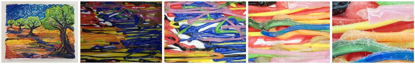
Figure 3. An artwork and original images, one from each elevation layer.

4.3 Qualitative

The purpose of qualitative experiments is twofold: first to test the applicability of the proposed approach in a diverse set of surface materials; second, to investigate the overall consistency of this approach concerning the large number of images utilized; and, third, to assess the limitations of the method due to the geometry of the target surfaces.

4.3.1 Structure and composition

Exploratory experiments with surfaces made from different types of materials are presented. The rationale of this experiment is to assess the capability of the scanning method in materials of different reflectance properties.

4.3.1.1 Materials

The following surfaces were scanned, ranging in levels of shininess and texture. In all cases, the scanner area was 4 × 3cm².

Two pieces of medium-density fiber (MDF) wood board, g₁ and g₂, with carvings each made with a Dremel rotary tool mounted with a 2-mm cutting disk. In addition, piece g₂ has a coarser marking made by dragging the rotating tool across the surface. Part g₂ had some scribbles done with a blue ballpoint pen at its top-right corner. The cuts were up to 2.5 mm deep. Both pieces were matte. The texture was light but sufficient; the ballpoint pen markings enhanced it (see Figure 4, second from left).

Figure 4

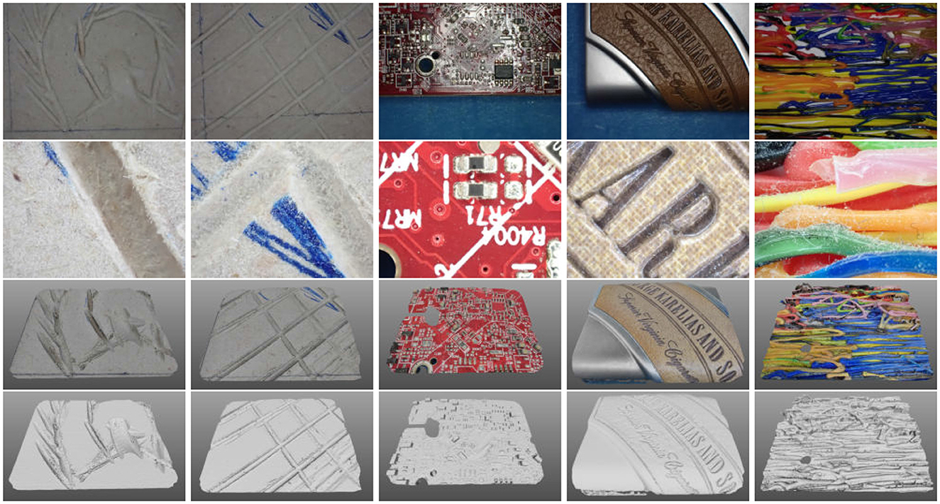
Figure 4. Rows, top to bottom: original images of targets g₁ to g₅, respectively, from left to right, from the top elevation layers; original images of targets g₁ to g₅ from the bottom elevation layers, in the same order; textured reconstructions of targets g₁ to g₅, respectively, from left to right; untextured reconstructions of targets g₁ to g₅, in the same order.

An integrated circuit board, g₃, is made from mainly shiny materials, that is, copper, solder, silkscreen, and glass fiber. The highest parts of the board were 1.5 mm from the glass fiber surface of the board. As evidenced in the middle column of Figure 4, the board was shiny in general and specifically at the regions of the flat, highly reflective glass fiber board. Texture was available in general but absent in some regions of the board.

An artwork (painting) made from 1.75-mm threads of polylactic acid,³ g₄; this is the same object as in Figure 3. For the application of the thermoplastic on the artwork surface, a 3D pen with a 0.7-mm nozzle was used. The height variability was approximately 3 mm, but a couple of individual threads extended up to 8 mm from the surface. Most importantly, this target was not a surface but an assembly of PLA threads; in some cases, one thread could be suspended above others at a height of a few millimeters. The texture is dense, but the top of the plastic filament is shiny at all ranges, even the closest ones.

A composite surface, g₅, made from a piece of aluminum and a piece of synthetic leather, the latter embossed. The synthetic leather material was moderately shiny and textured. The height variability was approximately 3 mm. The aluminum was shiny and with poor texture. Original images from the top and bottom layers are shown in Figure 4, along with corresponding reconstruction results.

No post-processing (e.g., smoothing, hole filling, normal correction, etc.) was applied in the results shown in the following discussion.

4.3.1.2 Observations

The reconstruction of g₁ and g₂ did not exhibit issues. Despite the MDF surface appearing textureless to the eye in far-range images, in close-range imaging, the faint structure shown in Figure 4 gives rise to feature detection.

The reconstruction of g₃ exhibited a hole at the location of a region that contained solely fiber glass. At the corresponding region, the sparse reconstruction has a relatively lower density of feature points. Similarly, at the same region, the original images exhibit a lack of texture and aperture problems compared to the rest of the image. In the top row of Figure 5, shown are five images that assist this observation, from left to right. The left is a 2D mosaic of images overviewing the surface, computed as by Zabulis et al. (2021); it is shown as a reference. The second is the top view of the surface reconstruction. The third shows the reconstructed reference points in the sparse reconstruction; the hole region is indicated with a dashed rectangle. The fourth image is a magnification of the third in the area of the dashed rectangle. The fifth is an original image from the closest layer, centered above the hole region.

Figure 5

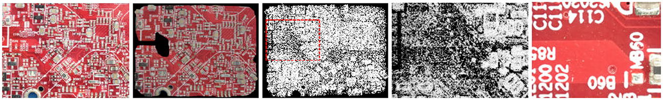
Figure 5. Left to right: two-dimensional mosaic of scanned surface; parse reconstruction of g₃; detail at the hole region; original image centered at the hole region.

Although the reconstruction of g₄ appears complete from the top, in Figure 6, missing surface texture and gross geometric inaccuracies are visible when the reconstruction is viewed laterally. The reason is that the scanned structure is more complex to be characterized than a surface because it contains filament threads suspended one above the other, leaving void space between them. As such, there are artifact locations that are not visible to the camera. Such an occasion is shown in Figure 6, where a pink thread is suspended above a green thread. In the figure, the same detail of the reconstruction is shown from a top and a lateral viewpoint in two pairs of images. The left pair shows the reconstruction detailed, textured, and untextured, from a top view. The right pair shows the same detail, from a lateral view, textured, and untextured. In the lateral view, it is observed that the void between the bottom and the suspended filament is reconstructed. The structure however at regions not visible to the camera (underside of the suspended filament) is grossly inaccurate. The same regions are textured with black, as they do not appear in any image in the data.

Figure 6

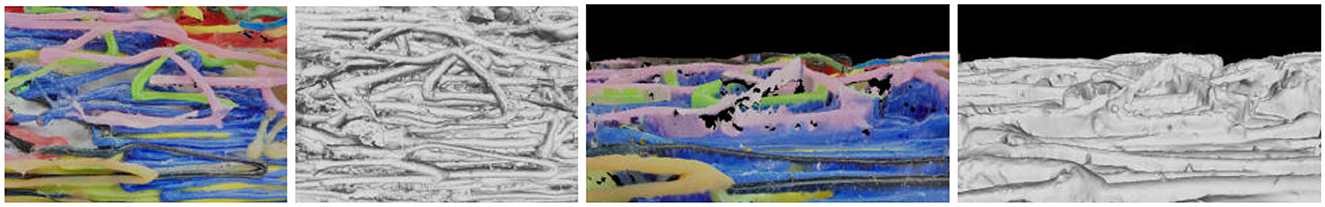
Figure 6. Details of the reconstruction of g₄, from a top (left) and lateral view (right).

In g₅, the shiny aluminum surface gives rise to texture, due to the minute surface structure that is visible at that close range.

4.3.1.3 Discussion

Automated scanning and close-range photogrammetry are sufficient for the photorealistic and fairly accurate reconstruction at very high detail.

4.3.1.3.1 Close-range imaging

When imaged in close range, surfaces exhibit less specularities and reveal texture, due to natural wear or inherent structure. Systematic image acquisition makes more probable the imaging of structure without specular artifacts, such as in the case of aluminum in g₅. Still, in g₃, the impeccability of the industrial and coated fiber glass hinders the method.

4.3.1.3.2 Lack of texture and visibility

The shortcomings in g₃ and g₄ are known limitations of photogrammetry. Conventional methods for their solution require the photogrammetric measurement of such regions and structured lighting to create texture and the acquisition of more views to fully cover the structure. The first is possible as a source of structured light can be mounted on the implemented set-up. The second would require a more flexible motorization mechanism. They are both left for future work.

4.3.1.3.3 Scope

The image acquisition locations in this work are unable to reach surface regions that are not visible from top views, as in the example of g₄. Although some of the structure is reconstructed this approach cannot guarantee the coverage of structures that are more complex than anaglyphs. As such, the recommended domain of the proposed approach is set in surface scanning. This is the reason that the approach is characterized as a surface scanning method in the title of this article.

4.3.2 Global consistency

This experiment indicates the contribution of far-range images to the accuracy of the reconstruction result. As discussed in Section 3.5.2, photogrammetry with large numbers of images is prone to camera pose estimate error accumulation, resulting in reconstruction inaccuracies. To illustrate this point, this experiment uses the same images, as acquired by the proposed method, but in two basic conditions and an additional one. In the first condition (C1), the proposed method is utilized. In the second condition (C2), the same images were inputted to the Pix4D photogrammetric suite. In the additional condition (C3), we used a state-of-the-art variant (Kerbl et al., 2023) of the neural radiance fields (NeRFs) method (Mildenhall et al., 2020), which was also fed with the same images. Indeed, NeRFs are targeted at learning the radiance field, rather than achieving a geometric reconstruction. That is, NeRFs are not destined for measurements but for view synthesis. Still, they are quite useful when 3D visualization is the application goal.

The reconstruction target was a handcrafted engraving at the end of the handle of a silver spoon. The engraving occupies an area of 45 × 25mm². In Figure 7 (top row), this item is shown from a top and a side view. It is observed that the spoon is undamaged and that its handle at the location of the engraving is straight.

Figure 7

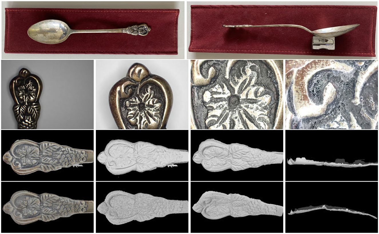
Figure 7. Rows, top to bottom: top and side views of a handcrafted silver spoon, on the left and right column, respectively; original images, one from each elevation later, from left to right; reconstruction using proposed method (C1); reconstruction using an off-the-shelf photogrammetric suite (C2).

In Figure 7, indicative original images and the obtained reconstructions are shown. The second row of Figure 7 shows one image from each elevation layer. The third and fourth rows show the result of C1 and C2, respectively, and in the following way: The left column shows the frontal views of the textured reconstructions. The rest of the columns show only their geometrical, untextured structure. Specifically, the second column from the left shows frontal views. The second column from the right shows slanted views (30°). The right column shows side views (90°).

Global accuracy improvements are observed in the side views, as in C2; the surface appears spuriously curved, while the original artifact is straight; see Figure 7 (top row, right). In C1, this effect is reduced. This improvement is attributed to the utilization of feature tracks over the far-range images and their contribution to better camera pose estimation, which leads to a more consistent reconstruction. This is attributed to the contribution of the far-range views constraint the accumulation of camera pose estimation errors.

The comparison between the two reconstruction approaches is not entirely fair, as different pre- and post-processing pipelines are followed in C1 and C2. To add to this unfairness, C2 is not programmed to search for medial correspondences as the proposed image acquisition approach is not guaranteed in generic photogrammetry implemented by off-the-shelf photogrammetric suites. The experiment provides the finding that the additional constraints provided by tracking features across distances are to the benefit of reconstruction quality.

The result of C3 is shown in Figure 8. As expected, the photometric appearance of the NeRF reconstruction; that is, the colors in the reconstruction look more vivid. However, when its structure is inspected, it is observed that the surface structure is only coarsely captured. In defense of the NeRF method, the recommended image acquisition for its optimal use is different from ours and requires the acquisition of views around the object. However, this would require a significant change in the hardware and increase the cost of the devices while still not providing fine structural measurements.

Figure 8

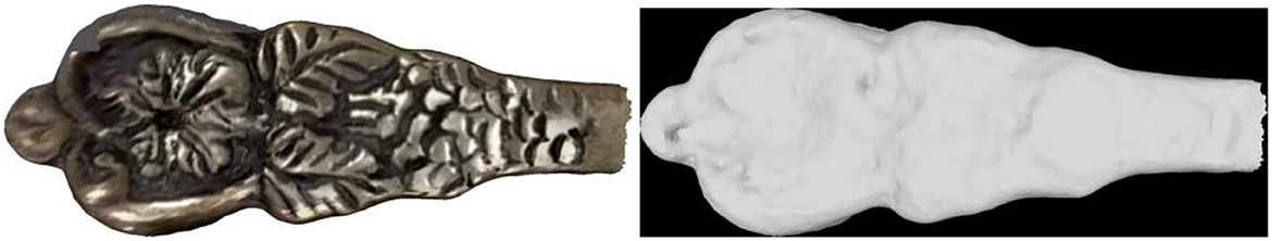
Figure 8. Reconstruction results of the artifact in Figure 7, using the methods from Kerbl et al. (2023), for condition C3. Left: top view of the textured reconstruction. Right: top view of the untextured reconstruction.

4.3.3 Shiny, curved, and sharp surfaces

Stereo vision and photogrammetry are usually incapable of reconstructing even moderately shiny surfaces. The reason is that they reflect different parts of the environment from each viewpoint, and thereby, the “uniqueness constraint” (Marr and Poggio, 1976) is not met. This incapability has been countered by the employment of additional algorithmic methods, such as photometric stereo (Karami et al., 2022), which requires additional and high-end hardware and illumination, the application of matting spray (Petruccioli et al., 2022), or manual editing (Nicolae et al., 2014). A study demonstrating the problems caused by highly reflective surfaces in multiple 3D reconstruction modalities, including photogrammetry, can be found in Michel et al. (2014). However, when the imaging range is very close, even shiny surfaces contain some texture. The purpose of the experiment is to assess reconstruction quality for metallic surfaces and find the limits of the proposed configuration of this type of surface.

Shiny metallic nuts and screws were scanned because they feature multiple orientations and curvatures. These structural features are susceptible to illumination artifacts because they reflect light from multiple directions. Some of these structures are higher than the depth-of-focus range of the camera. For this reason, coarse sand was used as a substrate and the targets were partially submerged in it to study the upper surface of these structures. Original images are shown in the top two rows of Figure 9.

Figure 9

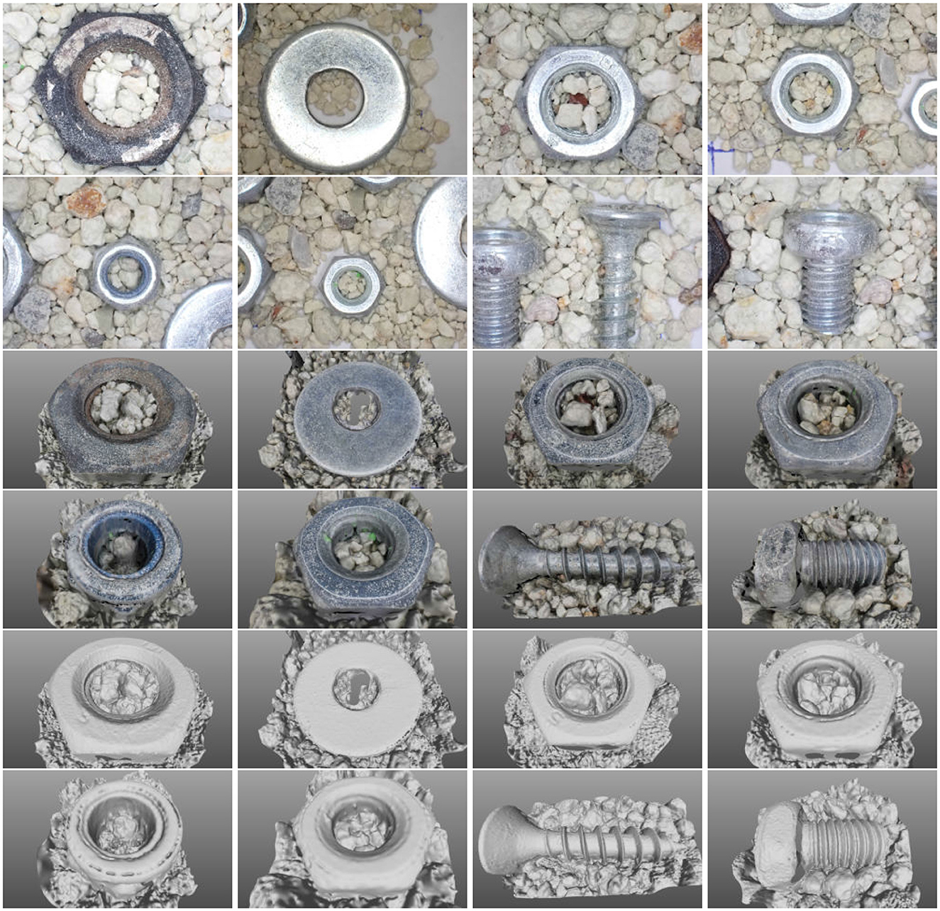
Figure 9. Top two rows: original images of metallic nuts and screws from the top layer. Middle two rows: textured reconstructions of the metallic nuts and screws in the top two rows. Bottom two rows: untextured renderings of the reconstructions in the two middle rows.

The images exhibit specular reflectances that are reduced with imaging distance. Surface regions that contain such reflectances are constrained to the high curvature parts of the surface such as the creases of the bolts and the railings of the screws. In the images, these specularities are expressed as saturated (white) regions of pixels at the high curvature regions. Still, small imperfections, dust particles, and structural features give rise to some feature correspondences.

The obtained reconstructions are shown, in the same order, in the four bottom rows of Figure 9. It is observed that the reconstructions do not suffer from gross structural errors. It is furthermore observed that surface patterns are reconstructed, such as screw threads and bolt markings. However, when specular reflections are systematic over broad regions of pixels, the reconstruction exhibits artifacts that occur exactly at the high-curvature regions of the surface.

To compare against conventional photogrammetry, we have reconstructed the same scene using the Pix4D software and present the results in Figure 10 (left). As can be observed, very little of the scene is reconstructed. To indicate the difference with the proposed method in Figure 10 (right), the sparse reconstruction of the scene using the proposed method, from the same viewpoint, is also shown. It is observed that the reconstruction obtained using Pix4D is poor and manages to reconstruct only a few parts of the scene. The reason is the lack of correspondences and the establishment of many erroneous correspondences due to the shiny material of the targets.

Figure 10

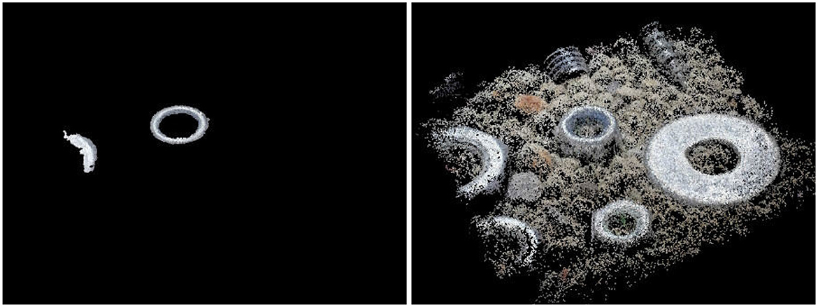
Figure 10. Left: reconstruction of a scene with shiny objects using Pix4D. Right: sparse reconstruction of the same scene using the proposed method.

4.4 Quantitative

To measure the accuracy of reconstruction, targets of known size and structural features are utilized. To the best of our knowledge, there exists no benchmark for close-range photogrammetry at the scale dealt with by this work in general and in particular for the specific image acquisition approach proposed. Therefore, we have used coins as reference targets so that other works can compare the same or analogous structures. Two experiments are reported that assess metric errors and global distortions.

4.4.1 Dimensions

The purpose of the experiment was to measure reconstructed dimensions and compare them with the ground truth.

State-manufactured coins were used because they are of standard size and very accurately manufactured to avoid counterfeiting. The scanned coins belong to the euro currency. All eight coins from this family were scanned and placed on a planar and textured surface. In addition, to the nominal dimensions provided by the manufacturer, the coins were measured with an electronic caliper. No larger than a 0.01-mm difference was found in these measurements. The measured dimensions were considered ground truth as the coins were used and may have suffered distortions. The digital models are in metric units, and their dimensions were compared to the ground-truth dimensions of the coins. Their discrepancy is the measurement error.

Original images are shown in Figure 11. The top two rows show images from the highest elevation layer and the other two images from the lowest layer. The corresponding reconstructions are shown, in the same order, in Figure 12.

Figure 11

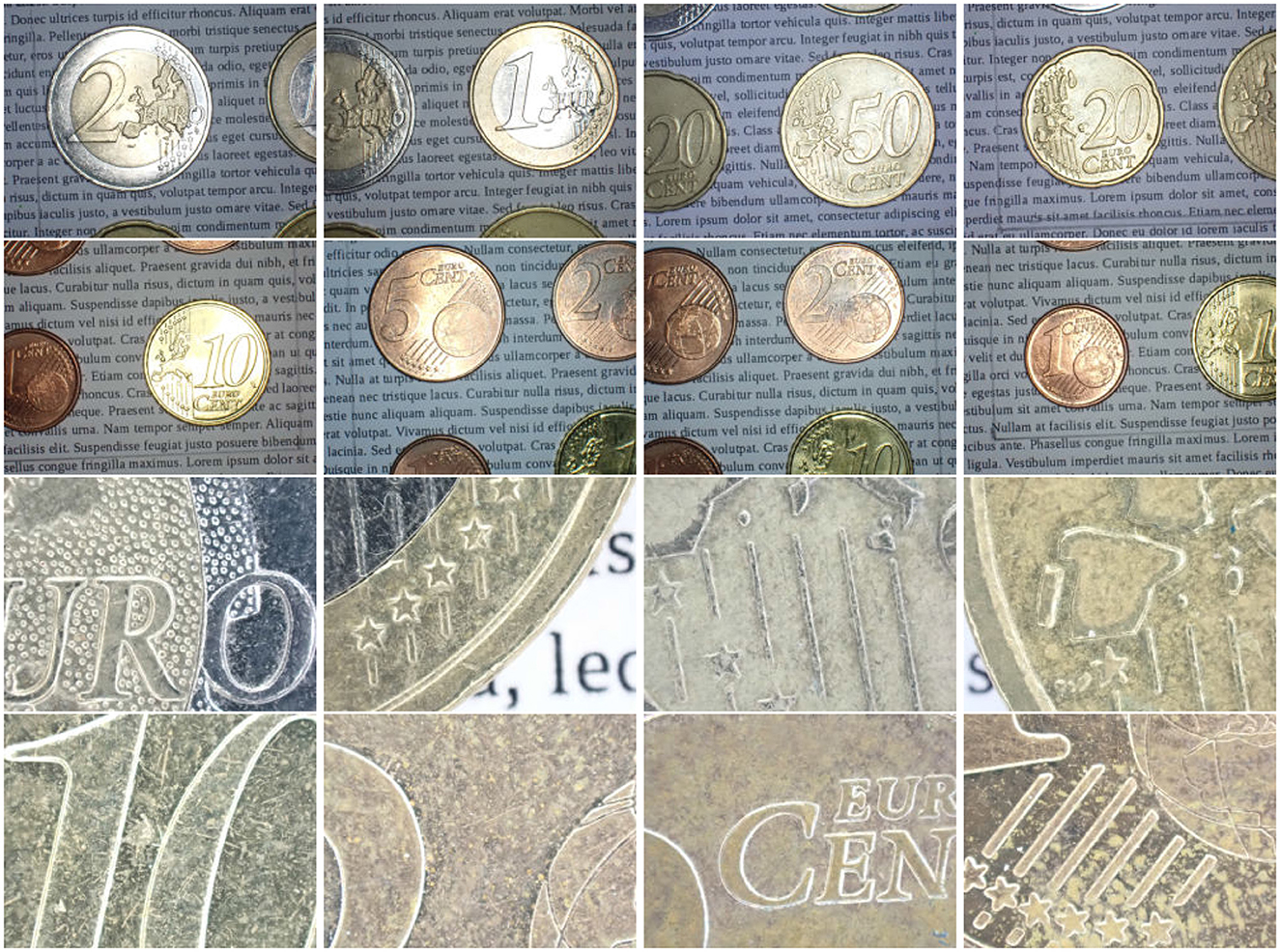
Figure 11. Original images of circular coins. The top couple of rows shows an original image of the target from the top layer. The bottom couple of rows shows an original image from the closest layer to the target.

Figure 12

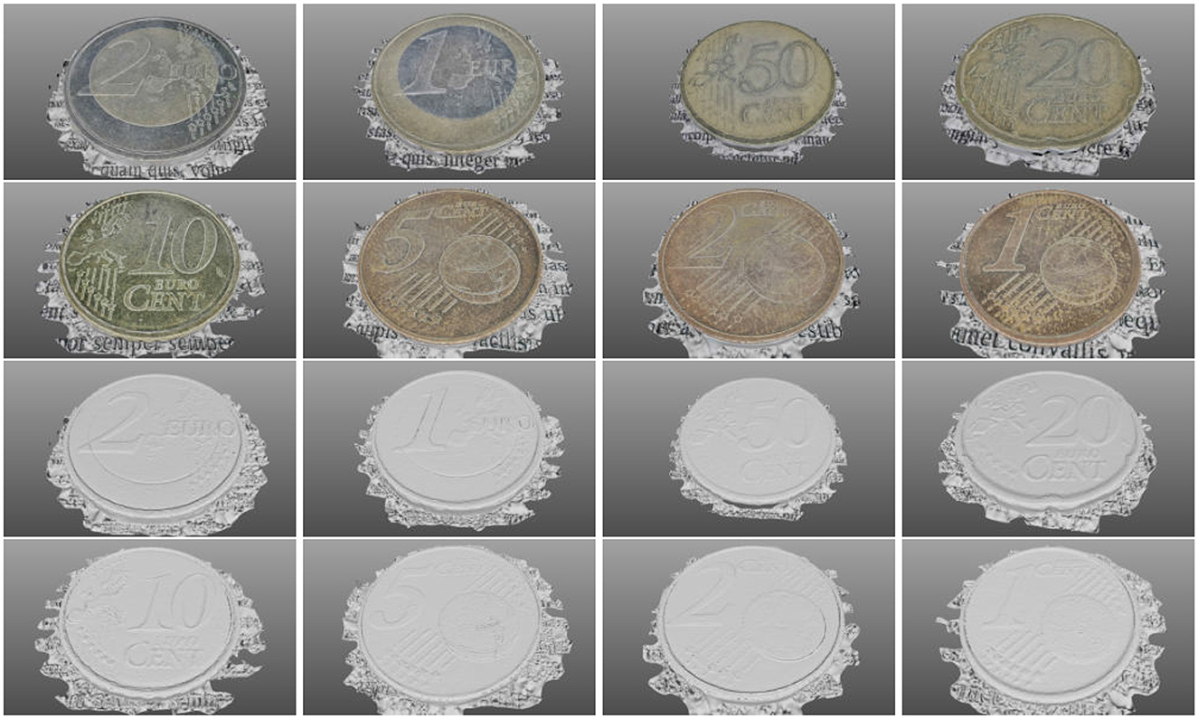
Figure 12. Reconstructions of the circular coins shown in Figure 11. The top couple of rows shows the textured reconstructions. The bottom couple of rows shows the untextured reconstructions from the same viewpoints.

The dimensions and errors are reported in Table 1. The first column notes the currency value. The column “Nominal” reports the dimensions provided by the manufacturer (European Central Bank), the column “Measured” reports our caliper measurements (ground truth), the column “Measurement” reports the dimensions of the digital model, and the column “Error” is the percentage error. The thickness of the coins was measured as the distance of the supporting plane to the top face of the reconstruction. The average measurement error is approximately 2.91%.

Table 1

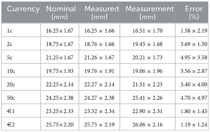
Table 1. Coin dimensions (diameter × thickness): nominal, measured, and reconstruction errors.

4.4.2 Aspect ratio

The purpose of this experiment is to measure any deviation from the circular shape of coin edges to assess global distortions in the reconstruction.

To assess global distortions in the reconstruction, the orthoimages of the coin reconstructions were used. These orthoimages are perpendicular projections of the reconstruction upon a hypothetical plane parallel to the surface. These images are “map-accurate” in that they do not contain perspective distortions included in the original photographs. Depth maps computed for orthophotos share also this property.

The depth map for an orthophoto of a frontal view of the reconstruction was computed using z-buffering (Catmull, 1974). Canny edge detection (Canny, 1986) was performed in that map, detecting depth discontinuities. Circles were robustly detected using RANSAC to eliminate outlier edges. The inlier edges, E_in, were used to fit circles, using least squares. In Figure 13, shown are the inlier depth edges E_in superimposed on the orthoimages of the textured reconstructions.

Figure 13

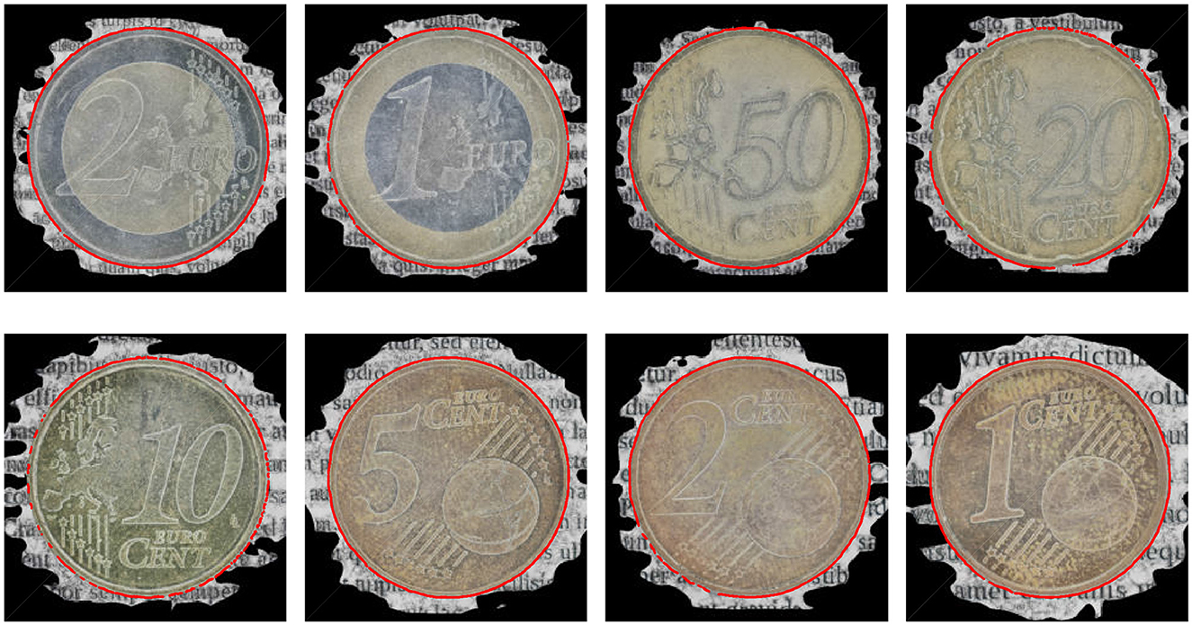
Figure 13. Orthoimages of textured reconstructions superimposed with the depth edges employed in the assessment of reconstruction distortions.

In Table 2, deviations of the detected edges from the fitted circle are reported as the mean distance of these edges from the fitted circle and their standard deviation. The small deviations and the visual results indicate that the circles were appropriately fitted. The average error is approximately 0.58 pixels.

Table 2

Table 2. Radius, mean circle fit error, and standard deviation for each measured coin.

Given the representativeness of the circle, the aspect ratio of the detected points is computed to assess whether the reconstruction is isotropic. To compute this the leftmost (p₁), rightmost (p₂), top (p₃), and bottom (p₄) points of inliers E_in were found. Then, aspect ratio |p₂−p₁|/|p₄−p₃| is an indicator of anisotropy over the horizontal and vertical surface dimensions. The last column of Table 2 reports these ratios, indicating a mean aspect ratio of 0.998 or a 0.0018% deviation from isotropy.

4.4.3 Surface structure

The purpose of this experiment is to assess the accuracy of the reconstruction of surface structure. To achieve this, we used the digitisation of a coin by a scanner, which is more accurate than photogrammetry, and used that digitisation as ground truth. By comparing this higher accuracy model, we obtain a measure of the accuracy of our method. To quantify the error of the proposed method, we used cross-correlation to measure the similarity between two depth maps. To measure the similarity of the depth edges in these maps, we have used the Hausdorff distance (Hausdorff, 1914), which is a metric that quantifies the similarity between two sets of points or shapes.

The proposed method and the Pix4D reconstruction of a €2 coin were compared to a higher-quality scan of the coin. This higher-quality scan was produced by the TetraVision company using an elaborate scanning technique that involved binocular (stereo) imaging and structured light, using the “Atos III Triple Scan” 3D scanner manufactured by the GOM company. This data set is available from TetraVision (2024). The coin was clamped in a fixture with reference points to ease the registration of partial scans, and the scanning mechanism included an automated tilt-and-swivel unit to image the coin from different angles. In addition, the coin was covered in a water-based transparent anti-reflex spray. The three scans were named S₁ for the proposed method, S₂ for the Pix4D reconstruction, and S₃ for the TetraVision reconstruction.⁴

The depth maps of the three scans were produced and the top surface region of the coin was isolated to compare the same surface regions. In these maps, the following measurements were acquired. First, we computed the cross-correlation between image pairs (S₁, S₃) and (S₂, S₃), which were 99.84% and 86.43%, respectively. Second, we performed Canny edge detection (Canny, 1986) on all three maps using the same parameters. The spatial arrangements of the obtained edges were compared using the Haussdorf distance for the same image pairs. The results were 73.53 p and 110.63 p for image pairs (S₁, S₃) and (S₂, S₃), respectively. In Figure 14, the textureless reconstructions and the edge detection results are shown.

Figure 14

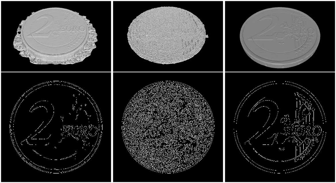
Figure 14. Top: surface reconstructions of a €2 coin. Bottom: edge detections on the depth maps of the reconstructions. Left to right: proposed method, Pix4D, and ground truth.

Qualitatively, the comparison of S₁ with S₂ offers similar observations as those obtained in Section 4.3.2; that is, S₂ exhibits significant levels of noise. This is also observed by the structure of edges in Figure 14 (bottom, middle). Quantitatively, both the correlation and the Haussdorf measures of dissimilarity indicate the greater accuracy of the proposed method as it provides more similar results to S₃.

4.5 Discussion

4.5.1 Scope and specifications

The proposed approach was evaluated in a wide range of materials. As expected, the accuracy of the method is best in textured and matte surfaces. The proposed approach exhibits robustness to moderately shiny surfaces but less robustness to lack of texture—a problem that is common to all photogrammetric methods. The proposed approach is not suitable for the reconstruction of reflective, transparent, or translucent surfaces.

The obtained resolutions are approximately 714p/mm² or approximately 679ppi for the geometry and approximately 257Kp/mm² or approximately 13Kdpi for texture.

4.5.2 Limitations

The limits of the proposed scanner lie within the depth of field of the camera and the memory capacity of the utilized computer.

The proposed approach is limited by the depth of field of the visual sensor, which for consumer-grade cameras is 1 cm. Images of scenes that contain depth variability exceeding this limit are not fully focused. Thereby, unfocused areas will not be accurately reconstructed or reconstructed at all.

Memory capacity is pertinent to the surface area that can be reconstructed as the wider this area is, the more images are required and more key point features need to be stored in memory. Using a modest computer, the scanning area achieved is 5cm², which is wider than the approaches presented in Section 4.2, which achieve scanning areas in the range of approximately 1-2 cm². It ought to be noted that the limits of the approaches in Section 4.2 were due to motorization, algorithmic, or optical constraints. In contrast, wider areas can be reconstructed using the proposed approach if more memory is available.

5 Conclusion

A surface reconstruction approach and its implementation are proposed in the form of a surface scanning modality. The proposed approach employs image acquisition at multiple distances and feature tracking to increase reconstruction accuracy. The resultant device and approach offer a generic surface reconstruction modality that is robust to illumination specularities, is useful for several applications, and is cost-efficient.

This work can be improved in two ways: first, by using structured lighting to counter the lack of texture, which would necessitate the use of additional hardware or images (see Section 2.2.4), and, second, by relaxing the limitation imposed by the restricted depth of focus range (1 cm in our case) of the optical sensor. By revisiting the focused sstacking method described in Section 4.1, it is possible to acquire images at several distances and use the depth from focus visual cue (Grossmann, 1987) to coarsely approximate the elevation map of the surface. This approximation can be then used to scan the surface in a second pass, guiding the camera elevation appropriately so that the surface occurs within its depth of focus.

Data availability statement

The datasets presented in this study can be found in online repositories. The names of the repository/repositories and accession number(s) can be found in the article/Supplementary material. The surface reconstructions presented in this work can be found at https://doi.org/10.5281/zenodo.8163498 and https://doi.org/10.5281/zenodo.8359465.

Author contributions

PK: Methodology, Software, Validation, Visualization, Writing – original draft. XZ: Conceptualization, Funding acquisition, Methodology, Project administration, Supervision, Visualization, Writing – original draft, Writing – review & editing. NS: Conceptualization, Data curation, Methodology, Software, Writing – original draft. NP: Funding acquisition, Investigation, Methodology, Project administration, Supervision, Writing – original draft. EZ: Investigation, Project administration, Resources, Writing – original draft. ID: Formal analysis, Project administration, Validation, Writing – review & editing.

Funding

The author(s) declare financial support was received for the research, authorship, and/or publication of this article. This work was supported by the Research and Innovation Action, Craeft, Grant No. 101094349, funded by the Horizon Europe Programme of the European Commission.

Conflict of interest

The authors declare that the research was conducted in the absence of any commercial or financial relationships that could be construed as a potential conflict of interest.

Publisher's note

All claims expressed in this article are solely those of the authors and do not necessarily represent those of their affiliated organizations, or those of the publisher, the editors and the reviewers. Any product that may be evaluated in this article, or claim that may be made by its manufacturer, is not guaranteed or endorsed by the publisher.

Abbreviations

b, byte; c, cent; CNC, Computer Numerical Control; CPU, Central Processing Unit; €, Euro; FoV, Field of View; G-code, Geometric Code; GHz, gigahertz; GPU, Graphics Processing Unit; JPEG, Joint Photographic Experts Group; Mp, megapixel; NeRF, Neural Radiance Field; p, pixel(s); ppi, points per inch; PNG, Portable Network Graphics; PLA, Polylactic acid; PLY, Polygon File Format; RAM, Random-Access Memory.

Footnotes

1. ^G-code, or RS-274, is a programming language for numerical control, standardized by ISO 6983.

2. ^PLY, or Stanford Triangle Format, is a format to store 3D data from scanners.

3. ^Polylactic acid (PLA) is an easy-to-process biocompatible, biodegradable plastic, used as 3D printer filament.

4. ^S₁ is the same reconstruction with that presented in Figure 12.

References

Barnes, C., Shechtman, E., Finkelstein, A., and Goldman, D. B. (2009). Patchmatch: a randomized correspondence algorithm for structural image editing. ACM Trans. Graph. 28, 24. doi: 10.1145/1531326.1531330

Crossref Full Text | Google Scholar

Besl, P., and McKay, N. D. (1992). A method for registration of 3-D shapes. IEEE Trans. Patt. Analy. Mach. Intell. 14, 239–256. doi: 10.1109/34.121791

Crossref Full Text | Google Scholar

Canny, J. (1986). A computational approach to edge-detection. IEEE Trans. Patt. Analy. Mach. Intell. 8, 679–698. doi: 10.1109/TPAMI.1986.4767851

Crossref Full Text | Google Scholar

Catmull, E. (1974). A Subdivision Algorithm for Computer Display of Curved Surfaces. Ann Arbor, MA: The University of Utah.

Google Scholar

Cernea, D. (2008). OpenMVS: Multi-view stereo reconstruction library. Available online at: https://cdcseacave.github.io/openMVS (accessed June 6, 2023).

Google Scholar

Cheng, J., Leng, C., Wu, J., Cui, H., and Lu, H. (2014). “Fast and accurate image matching with cascade hashing for 3D reconstruction,” in IEEE Conference on Computer Vision and Pattern Recognition, 1–8. doi: 10.1109/CVPR.2014.8

Crossref Full Text | Google Scholar

Csurka, G., Zeller, C., Zhang, Z., and Faugeras, O. (1997). Characterizing the uncertainty of the fundamental matrix. Comput. Vision Image Underst. 68, 18–36. doi: 10.1006/cviu.1997.0531

Crossref Full Text | Google Scholar

Davies, A. (2012). Close-Up and Macro Photography. Boca Raton, FL: CRC Press. doi: 10.4324/9780080959047

Crossref Full Text | Google Scholar

Dong, Y., Fan, G., Zhou, Z., Liu, J., Wang, Y., and Chen, F. (2021). Low cost automatic reconstruction of tree structure by adqsm with terrestrial close-range photogrammetry. Forests 12, 1020. doi: 10.3390/f12081020

Crossref Full Text | Google Scholar

Eldefrawy, M., King, S., and Starek, M. (2022). Partial scene reconstruction for close range photogrammetry using deep learning pipeline for region masking. Rem. Sens. 14, 3199. doi: 10.3390/rs14133199

Crossref Full Text | Google Scholar

Espuny, F., Monasse, P., and Moisan, L. (2014). “A new a contrario approach for the robust determination of the fundamental matrix,” in Image and Video Technology-PSIVT 2013 Workshops (Berlin, Heidelberg: Springer), 181–192. doi: 10.1007/978-3-642-53926-8_17

Crossref Full Text | Google Scholar

Fang, K., Zhang, J., Tang, H., Hu, X., Yuan, H., Wang, X., et al. (2023). A quick and low-cost smartphone photogrammetry method for obtaining 3D particle size and shape. Eng. Geol. 322, 107170. doi: 10.1016/j.enggeo.2023.107170

Crossref Full Text | Google Scholar

Fau, M., Cornette, R., and Houssaye, A. (2016). Photogrammetry for 3D digitizing bones of mounted skeletons: potential and limits. Compt. Rendus Palevol. 15, 968–977. doi: 10.1016/j.crpv.2016.08.003

Crossref Full Text | Google Scholar

Fernández-Lozano, J., Gutiérrez-Alonso, G., Ruiz-Tejada, M. Á, and Criado-Valdés, M. (2017). 3D digital documentation and image enhancement integration into schematic rock art analysis and preservation: the castrocontrigo neolithic rock art (NW Spain). J. Cult. Herit. 26, 160–166. doi: 10.1016/j.culher.2017.01.008

Crossref Full Text | Google Scholar

Fischler, M., and Bolles, R. (1981). Random sample consensus: a paradigm for model fitting with applications to image analysis and automated cartography. Commun. ACM 24, 381–395. doi: 10.1145/358669.358692

Crossref Full Text | Google Scholar

Fua, P. (1993). A parallel stereo algorithm that produces dense depth maps and preserves image features. Mach. Vis. Applic. 6, 35–49. doi: 10.1007/BF01212430

Crossref Full Text | Google Scholar

Furtner, M., and Brophy, J. (2023). Preliminary comparison of close-range photogrammetric and microct scanning: surface deviation analysis of 3D digital models of hominin molar crowns. J. Archaeol. Sci. 47, 103762. doi: 10.1016/j.jasrep.2022.103762

Crossref Full Text | Google Scholar

Gajski, D., Solter, A., and Gašparovic, M. (2016). Applications of macro photogrammetry in archaeology. Int. Arch. Photogr. Rem. Sens. Spatial Inf. Sci. 41, 263–266. doi: 10.5194/isprsarchives-XLI-B5-263-2016

Crossref Full Text | Google Scholar

Gal, R., Wexler, Y., Ofek, E., Hoppe, H., and Cohen-Or, D. (2010). Seamless montage for texturing models. Comput. Graph. Forum 29, 479–486. doi: 10.1111/j.1467-8659.2009.01617.x

Crossref Full Text | Google Scholar

Galantucci, L., Guerra, M., and Lavecchia, F. (2018). “Photogrammetry applied to small and micro scaled objects: a review,” in International Conference on the Industry 4.0 Model for Advanced Manufacturing, eds. J. Ni, V. Majstorovic, and D. Djurdjanovic (Cham: Springer International Publishing), 57–77. doi: 10.1007/978-3-319-89563-5_4

Crossref Full Text | Google Scholar

Galantucci, L., Lavecchia, F., and Percoco, G. (2013). Multistack close range photogrammetry for low cost submillimeter metrology. J. Comput. Inform. Sci. Eng. 13, 044501. doi: 10.1115/1.4024973

Crossref Full Text | Google Scholar

Galantucci, L., Pesce, M., and Lavecchia, F. (2015). A stereo photogrammetry scanning methodology, for precise and accurate 3D digitization of small parts with sub-millimeter sized features. CIRP Ann. 64, 507–510. doi: 10.1016/j.cirp.2015.04.016

Crossref Full Text | Google Scholar

Galantucci, L., Pesce, M., and Lavecchia, F. (2016). A powerful scanning methodology for 3D measurements of small parts with complex surfaces and sub millimeter-sized features, based on close range photogrammetry. Prec. Eng. 43, 211–219. doi: 10.1016/j.precisioneng.2015.07.010

Crossref Full Text | Google Scholar

Gallo, A., Muzzupappa, M., and Bruno, F. (2014). 3D reconstruction of small sized objects from a sequence of multi-focused images. J. Cult. Herit. 15, 173–182. doi: 10.1016/j.culher.2013.04.009

Crossref Full Text | Google Scholar

González, M., Yravedra, J., González-Aguilera, D., Palomeque-González, J., and Domínguez-Rodrigo, M. (2015). Micro-photogrammetric characterization of cut marks on bones. J. Archaeol. Sci. 62, 128–142. doi: 10.1016/j.jas.2015.08.006

Crossref Full Text | Google Scholar

Grossmann, P. (1987). Depth from focus. Patt. Recogn. Lett. 5, 63–69. doi: 10.1016/0167-8655(87)90026-2

Crossref Full Text | Google Scholar

Guidi, G., and Shafqat, M.U M L. L. (2020). Optimal lateral displacement in automatic close-range photogrammetry. Sensors 20, 6280. doi: 10.3390/s20216280

PubMed Abstract | Crossref Full Text | Google Scholar

Harbowo, D., Sitorus, J., Agustina, L., Muztaba, R., Julian, T., and Malasan, H. (2022). “3D modelling of meteorite from astomulyo village, lampung, indonesia by close range photogrammetry (crp) methods,” in IOP Conference Series: Earth and Environmental Science, 12003. doi: 10.1088/1755-1315/1047/1/012003

Crossref Full Text | Google Scholar

Hartley, R., and Zisserman, A. (2003). Multiple View Geometry in Computer Vision. New York, NY, USA: Cambridge University Press. doi: 10.1017/CBO9780511811685

Crossref Full Text | Google Scholar

Hassett, B., and Lewis-Bale, T. (2017). Comparison of 3D landmark and 3D dense cloud approaches to hominin mandible morphometrics using structure-from-motion. Archaeometry 59, 191–203. doi: 10.1111/arcm.12229

Crossref Full Text | Google Scholar

Hausdorff, F. (1914). Grundzüge der Mengenlehre. Leipzig: Verlag von Viet & Comp.

Google Scholar

Heikkila, J., and Silven, O. (1997). “A four-step camera calibration procedure with implicit image correction,” in IEEE Conference on Computer Vision and Pattern Recognition, 1106–1112.

Google Scholar

Hiep, V., Labatut, P., Pons, J., and Keriven, R. (2011). High accuracy and visibility-consistent dense multiview stereo. IEEE Trans. Patt. Analy. Mach. Intell. 34, 889–901. doi: 10.1109/TPAMI.2011.172

PubMed Abstract | Crossref Full Text | Google Scholar

Illerhaus, B., Jasiuniene, E., Goebbels, J., and Loethman, P. (2002). “Investigation and image processing of cellular metals with highly resolving 3D microtomography (uCT),” in Developments in X-Ray Tomography III, ed. U. Bonse (International Society for Optics and Photonics, SPIE), 201–204. doi: 10.1117/12.452846

Crossref Full Text | Google Scholar

Inzerillo, L. (2017). Smart sfm: salinas archaeological museum. Int. Arch. Photogram. Rem. Sens. Spatial Inform. Sci. 42, 369–374. doi: 10.5194/isprs-archives-XLII-2-W5-369-2017

Crossref Full Text | Google Scholar

Jancosek, M., and Pajdla, T. (2014). Exploiting visibility information in surface reconstruction to preserve weakly supported surfaces. Int. Schol. Res. Not. 2014, 98595. doi: 10.1155/2014/798595

PubMed Abstract | Crossref Full Text | Google Scholar

Jiang, Y., Shi, H., Wen, Z., Guo, M., Zhao, J., Cao, X., et al. (2022). A comparative experimental study of rill erosion on loess soil and clay loam soil based on a digital close-range photogrammetry technology. Geomorphology 419, 108487. doi: 10.1016/j.geomorph.2022.108487

Crossref Full Text | Google Scholar

Jylänki, J. (2010). A thousand ways to pack the bin-a practical approach to two-dimensional rectangle bin packing. Available online at: https://github.com/juj/RectangleBinPack/blob/master/Readme.txt (accessed December 6, 2023).

Google Scholar

Karami, A., Menna, F., and Remondino, F. (2022). Combining photogrammetry and photometric stereo to achieve precise and complete 3D reconstruction. Sensors 22, 8172. doi: 10.3390/s22218172

PubMed Abstract | Crossref Full Text | Google Scholar

Kerbl, B., Kopanas, G., Leimkühler, T., and Drettakis, G. (2023). 3D gaussian splatting for real-time radiance field rendering. ACM Trans. Graph. 42, 1–14. doi: 10.1145/3592433

Crossref Full Text | Google Scholar

Kurniawan, A., Chusida, A., Utomo, H., Marini, M., Rizky, B., Prakoeswa, B., et al. (2023). 3D bitemark analysis in forensic odontology utilizing a smartphone camera and open-source monoscopic photogrammetry surface scanning. Pesquisa Brasil. Odontopediatr. Clín. Integr. 23, e220087. doi: 10.1590/pboci.2023.001

Crossref Full Text | Google Scholar

Lauria, G., Sineo, L., and Ficarra, S. (2022). A detailed method for creating digital 3D models of human crania: an example of close-range photogrammetry based on the use of structure-from-motion (sfm) in virtual anthropology. Archaeol. Anthropol. Sci. 14, 42. doi: 10.1007/s12520-022-01502-9

Crossref Full Text | Google Scholar

Lavecchia, F., Guerra, M., and Galantucci, L. (2017). The influence of software algorithms on photogrammetric micro-feature measurement's uncertainty. Int. J. Advanced Manufact. Technol. 93, 3991–4005. doi: 10.1007/s00170-017-0786-z

Crossref Full Text | Google Scholar

Lavecchia, F., Guerra, M., and Galantucci, L. (2018). Performance verification of a photogrammetric scanning system for micro-parts using a three-dimensional artifact: adjustment and calibration. Int. J. Advanced Manufact. Technol. 96, 4267–4279. doi: 10.1007/s00170-018-1806-3

Crossref Full Text | Google Scholar

Lösler, M., Eschelbach, C., and Klügel, T. (2022). Close range photogrammetry for high-precision reference point determination. Cham: Springer. doi: 10.1007/1345_2022_141

Crossref Full Text | Google Scholar

Lourakis, M., and Argyros, A. (2009). SBA: a software package for generic sparse bundle adjustment. ACM Trans. Mathem. Softw. 36, 1–30. doi: 10.1145/1486525.1486527

Crossref Full Text | Google Scholar

Lourakis, M., and Zabulis, X. (2013). “Accurate scale factor estimation in 3D reconstruction,” in International Conference on Computer Analysis of Images and Patterns (Berlin, Heidelberg: Springer-Verlag), 498–506. doi: 10.1007/978-3-642-40261-6_60

Crossref Full Text | Google Scholar

Lowe, D. (2004). Distinctive image features from scale-invariant keypoints. Int. J. Comput. Vis. 60, 91–110. doi: 10.1023/B:VISI.0000029664.99615.94

Crossref Full Text | Google Scholar

Luhmann, T. (2010). Close range photogrammetry for industrial applications. ISPRS J. Photogr. Rem. Sens. 65, 558–569. doi: 10.1016/j.isprsjprs.2010.06.003

Crossref Full Text | Google Scholar

Lussu, P., and Marini, E. (2020). Ultra close-range digital photogrammetry in skeletal anthropology: a systematic review. PLoS ONE 15, e0230948. doi: 10.1371/journal.pone.0230948

Crossref Full Text | Google Scholar

Marr, D., and Poggio, T. (1976). Cooperative computation of stereo disparity. Science 194, 283–287. doi: 10.1126/science.968482

PubMed Abstract | Crossref Full Text | Google Scholar

Marziali, S., and Dionisio, G. (2017). Photogrammetry and macro photography. the experience of the MUSINT II project in the 3D digitizing process of small size archaeological artifacts. Stud. Dig. Herit. 1, 298–309. doi: 10.14434/sdh.v1i2.23250

Crossref Full Text | Google Scholar

Mathys, A., and Brecko, J. (2018). Focus Stacking. Amsterdam: Amsterdam University Press, 213–216. doi: 10.2307/j.ctt1xp3w16.22

Crossref Full Text | Google Scholar

Michel, D., Zabulis, X., and Argyros, A. (2014). Shape from interaction. Mach. Vis. Applic. 25, 1077–1087. doi: 10.1007/s00138-014-0602-9

Crossref Full Text | Google Scholar

Mildenhall, B., Srinivasan, P., Tancik, M., Barron, J., Ramamoorthi, R., and Ng, R. (2020). “Nerf: representing scenes as neural radiance fields for view synthesis,” in European Cconference in Computer Vision, 405–421. doi: 10.1007/978-3-030-58452-8_24

Crossref Full Text | Google Scholar

Moulon, P., Monasse, P., and Marlet, R. (2013). “Adaptive structure from motion with a contrario model estimation,” in Asian Conference in Computer Vision, eds. K. Lee, Y. Matsushita, J. Rehg, and Z. Hu (Cham: Springer), 257–270. doi: 10.1007/978-3-642-37447-0_20

Crossref Full Text | Google Scholar

Moulon, P., Monasse, P., Perrot, R., and Marlet, R. (2016). “OpenMVG: Open multiple view geometry,” in International Workshop on Reproducible Research in Pattern Recognition (New York, NY: Springer), 60–74. doi: 10.1007/978-3-319-56414-2_5

Crossref Full Text | Google Scholar

Nicolae, C., Nocerino, E., Menna, F., and Remondino, F. (2014). Photogrammetry applied to problematic artefacts. Int. Arch. Photogr. Rem. Sens. Spat. Inf. Sci. 40, 451–456. doi: 10.5194/isprsarchives-XL-5-451-2014

Crossref Full Text | Google Scholar

Paixão, A., Muralha, J., Resende, R., and Fortunato, E. (2022). Close-range photogrammetry for 3D rock joint roughness evaluation. Rock Mech. Rock Eng. 55, 3213–3233. doi: 10.1007/s00603-022-02789-9

Crossref Full Text | Google Scholar

Percoco, G., Guerra, M.S S, and Galantucci, L. M. (2017a). Experimental investigation on camera calibration for 3D photogrammetric scanning of micro-features for micrometric resolution. Int. J. Adv. Manuf. Technol. 91, 2935–2947. doi: 10.1007/s00170-016-9949-6

Crossref Full Text | Google Scholar

Percoco, G., Modica, F., and Fanelli, S. (2017b). Image analysis for 3D micro-features: A new hybrid measurement method. Prec. Eng. 48, 123–132. doi: 10.1016/j.precisioneng.2016.11.012

Crossref Full Text | Google Scholar

Percoco, G., and Salmerón, A. (2015). Photogrammetric measurement of 3D freeform millimetre-sized objects with micro features: an experimental validation of the close-range camera calibration model for narrow angles of view. Measur. Sci. Technol. 26, 095203. doi: 10.1088/0957-0233/26/9/095203

Crossref Full Text | Google Scholar

Petruccioli, A., Gherardini, F., and Leali, F. (2022). Assessment of close-range photogrammetry for the low cost development of 3D models of car bodywork components. Int. J. Inter. Des. Manuf. 16, 703–713. doi: 10.1007/s12008-022-00865-6

Crossref Full Text | Google Scholar

Rodríguez-Martín, M., and Rodríguez-Gonzálvez, P. (2019). Learning methodology based on weld virtual models in the mechanical engineering classroom. Comput. Applic. Eng. Educ. 27, 1113–1125. doi: 10.1002/cae.22140

Crossref Full Text | Google Scholar

Rodríguez-Martín, M., and Rodríuez-Gonzalvez, P. (2018). “Learning based on 3D photogrammetry models to evaluate the competences in visual testing of welds,” in IEEE Global Engineering Education Conference, 1576–1581. doi: 10.1109/EDUCON.2018.8363422

Crossref Full Text | Google Scholar

Scaggion, C., Castelli, S., Usai, D., and Artioli, G. (2022). 3D digital dental models' accuracy for anthropological study: Comparing close-range photogrammetry to μ-ct scanning. Digit. Applic. Archaeol. Cult. Herit. 27, e00245. doi: 10.1016/j.daach.2022.e00245

Crossref Full Text | Google Scholar

Semendeferi, K., Damasio, H., Frank, R., and Van Hoesen, G. (1997). The evolution of the frontal lobes: a volumetric analysis based on three-dimensional reconstructions of magnetic resonance scans of human and ape brains. J. Hum. Evol. 32, 375–388. doi: 10.1006/jhev.1996.0099

PubMed Abstract | Crossref Full Text | Google Scholar

Shortis, M., Bellman, C., Robson, S., Johnston, G., and Johnson, G. (2006). “Stability of zoom and fixed lenses used with digital slr cameras,” in ISPRS Symposium of Image Engineering and Vision Metrology, 285–290.

Google Scholar

Sims-Waterhouse, D., Bointon, P., Piano, S., and Leach, R. (2017a). “Experimental comparison of photogrammetry for additive manufactured parts with and without laser speckle projection,” in Optical Measurement Systems for Industrial Inspection X (International Society for Optics and Photonics, SPIE), 103290W. doi: 10.1117/12.2269507

Crossref Full Text | Google Scholar

Sims-Waterhouse, D., Piano, S., and Leach, R. (2017b). Verification of micro-scale photogrammetry for smooth three-dimensional object measurement. Measur. Sci. Technol. 28, 055010. doi: 10.1088/1361-6501/aa6364

Crossref Full Text | Google Scholar

TetraVision (2024). 3D scan of a 2 euro coin. Available online at: https://www.tetravision.be/portfolio-item/3d-scan-of-a-2-euro-coin/ (accessed December 6, 2023).

Google Scholar

Waechter, M., Moehrle, N., and Goesele, M. (2014). “Let there be color! large-scale texturing of 3D reconstructions,” in European Conference on Computer Vision (Cham: Springer International Publishing), 836–850. doi: 10.1007/978-3-319-10602-1_54

Crossref Full Text | Google Scholar

Wang, B., Pan, P., Xiao, Q., Luo, L., Ren, X., Jin, R., et al. (2018). “Seamless color mapping for 3D reconstruction with consumer-grade scanning devices,” in European Conference on Computer Vision Workshops 633–648. doi: 10.1007/978-3-030-11009-3_39

Crossref Full Text | Google Scholar

Yang, B., Schinke, J., Rastegar, A., Tanyeri, M., and Viator, J. (2023). Cost-effective full-color 3D dental imaging based on close-range photogrammetry. Bioengineering 10, 1268. doi: 10.3390/bioengineering10111268

PubMed Abstract | Crossref Full Text | Google Scholar

Yang, C., and Medioni, G. (1992). Object modelling by registration of multiple range images. Image Vis. Comput. 10, 145–155. doi: 10.1016/0262-8856(92)90066-C

Crossref Full Text | Google Scholar

Zabulis, X., Koutlemanis, P., Stivaktakis, N., and Partarakis, N. (2021). A low-cost contactless overhead micrometer surface scanner. Appl. Sci. 11, 6274. doi: 10.3390/app11146274

Crossref Full Text | Google Scholar

Zhang, Z. (1999). “Flexible camera calibration by viewing a plane from unknown orientations,” in IEEE International Conference on Computer Vision, 666–673.

Google Scholar