 Luis de la Higuera1†
 Martín López-García1*†
 Mario Castro1,2†
 Niloufar Abourashchi3
 Grant Lythe1
 Carmen Molina-París1
- 1Department of Applied Mathematics, School of Mathematics, University of Leeds, Leeds, United Kingdom
- 2Grupo Interdisciplinar de Sistemas Complejos and DNL, Universidad Pontificia Comillas, Madrid, Spain
- 3Department of Statistical Science, University College London, London, United Kingdom
The homeostasis of T cell populations depends on migration, division and death of individual cells (1). T cells migrate between spatial compartments (spleen, lymph nodes, lung, liver, etc.), where they may divide or differentiate, and eventually die (2). The kinetics of recirculation influences the speed at which local infections are detected and controlled (3). New experimental techniques have been developed to measure the lifespan of cells, and their migration dynamics; for example, fluorescence-activated cell sorting (4), in vitro time-lapse microscopy (5), or in vivo stable isotope labeling (e.g., deuterium) (6). When combined with mathematical and computational models, they allow estimation of rates of migration, division, differentiation and death (6, 7). In this work, we develop a stochastic model of a single cell migrating between spatial compartments, dividing and eventually dying. We calculate the number of division events during a T cell's journey, its lifespan, the probability of dying in each compartment and the number of progeny cells. A fast-migration approximation allows us to compute these quantities when migration rates are larger than division and death rates. Making use of published rates: (i) we analyse how perturbations in a given spatial compartment impact the dynamics of a T cell, (ii) we study the accuracy of the fast-migration approximation, and (iii) we quantify the role played by direct migration (not via the blood) between some compartments.
1. Introduction
T cells are descendants of bone marrow progenitors that migrated to the thymus and underwent processes of maturation, gene rearrangement and selection (8). The surface of a T cell is populated with tens of thousands of copies of a T-cell receptor. A repertoire of T cells is maintained in a mammal's body that enables recognition of and response to the many benign and pathogenic microorganisms that are encountered over its lifetime, although the T-cell receptor of any individual cell only recognizes a tiny fraction of them (9, 10). An individual T cell may circulate between different tissues of the body for months or years, never encountering cognate antigen. Their interactions with self antigens, generally weak, are occasionally strong enough to cause one round of cell division. Strong interaction between the T-cell receptor and non-self antigens, mounted on MHC on the surface of antigen-presenting cells in lymph nodes (11), initiates a programme of multiple rounds of cell division and phenotypic changes that generate effector and memory T cells with different lifetimes and migration patterns (2, 12–15).
Blood is a dynamic conduit through which T cells pass, in homeostasis and during immune responses (16). Blood is also the only tissue from which it is easy to obtain samples of T cells from healthy humans, although only about two percent of the body's T cells are in the blood at any one time (17, 18). The fraction of T cells found in a particular tissue depends on how likely a T cell is to enter the tissue and on how long it stays there. At any one time, for example, the fraction of T cells in lymph nodes and spleen is large, not because a T cell in the blood is most likely to go there, but because, when they do enter, they remain there a long time (3). Direct counts of T cell numbers in organs of mice are sometimes possible (19, 20); direct measurement of the kinetics of recirculation is more difficult. Mathematical models of the full kinetics of recirculation are the basis of a systematic extrapolation from measurements to residence times and migration probabilities.
Ganusov and Auerbach (3) constructed a model, based on experimental data, in which the migration history of a T cell consists of short intervals in the blood (less than a minute each) between longer sojourns in lung, liver, spleen and lymph nodes. We adopt their star-shaped migration topology pattern here. We also adopt a Markov description, in which the next event in the lifetime of a T cell (migration, division or death) is stochastic, but governed by parameters that depend only on the cell's current position. We treat a division event as the birth of one new cell, that follows the same rules as its mother, and a continuation of the life of another. In our modeling, we have in mind the homeostasis of naive CD4+ T cells, without explicitly taking the effect of aging (15, 19, 21) into account.
Novel labeling techniques are providing an increasing amount of information about recirculation and other properties at the single cell level (4–6), which lead to new hypotheses and new experiments aimed at elucidating the kinetic properties of a cell's journey. Techniques such as staining or barcoding are ideal for quantifying dynamics at the single cell level, since they are able to track individual cells, their interactions with the extra-cellular environment and other cells and to help understand single cell lifetime dynamics (22, 23).
Although they are able to provide a substantial amount of quantitative data, experimental techniques are still far from being able to provide a full picture of lymphocyte dynamics in vivo, even in mice (24, 25). Thus, a partnership between experimental and in silico approaches is required. Deterministic continuous time models (based on ordinary differential equations) are the usual approach to study the kinetics of cell recirculation (7, 26, 27) when describing large cell populations. On the other hand, these deterministic approaches can miss some crucial behavior due to the stochastic nature of cellular heterogeneity and cellular interactions (28, 29). Stochastic processes are more appropriate when studying observables at the single cell level, instead of at the population level (30, 31).
This work is inspired by these new experimental techniques, and by the work of Ganusov and Auerbach (3), where the authors analyse the kinetics of lymphocyte recirculation. Our aim is to show how new analytical approaches can be applied to these systems to study the stochastic journey of a single cell during its lifetime. Based on the assumption that there are many more migration events than division and death events, we propose a fast-migration approximation. Finally, we carry out a range of numerical experiments to test the approximation, and to show the impact that cellular events occurring in a given spatial compartment can have on the whole system.
2. Theory
2.1. Description of the General Model
We consider a model of a T cell that migrates between different spatial compartments, where it may divide one or more times, before ultimately dying. Inspired by the representation of Ganusov and Auerbach (3, Figure 2), these compartments can represent blood, lymph nodes, lung, liver, spleen and Peyer's patches. We denote the blood compartment by B and denote M additional compartments by {C1, …, CM} (see Figure 1).
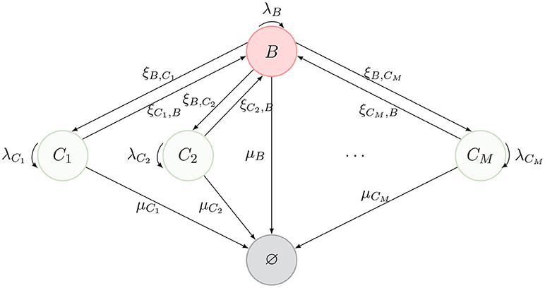
Figure 1. Schematic description of the model. The nodes represent spatial compartments where the CD4+ T cell can be located at a given time. The arrows connecting them represent the migration of the cell between compartments, with migration rates {(ξB,Cj, ξCj, B), j ∈ {1, …, M}}. Division events are represented by curved arrows with rates λB and {λCj, j ∈ {1, …, M}}. Finally, the state ∅ represents the death of the cell (with different death rates μB and {μCj, j ∈ {1, …, M}}, depending on the location where cell death takes place).
The journey of a T cell during its lifetime is summarized by the diagram in Figure 1. A cell can migrate between compartments, divide or die (reaching the state ∅). Our model is an absorbing continuous-time Markov chain (CTMC) defined on the space of states , where Y(t) identifies the position of the cell at time t ≥ 0. We note that division does not affect the position of the cell, Y(t), and therefore, we keep division events in our description as events that leave the process in the same state, as described in Figure 1. When tracking a given T cell, if a division event occurs, one of the two resulting cells is the daughter, while the other is taken to be the original cell.
Our aims are: (i) to show how the dynamics of a T cell (see Figure 1) can be studied by means of a number of summary statistics (or stochastic descriptors) in section 2.2, inspired by current single cell experimental techniques; (ii) to present in section 2.3 a fast-migration approximation which allows us to simplify the analysis when migration rates are much larger than division and death rates; and (iii) to quantify the impact of changes occurring in a single spatial compartment (section 3).
2.2. Single Cell Descriptors
Recent studies have highlighted the importance of improving the existing experimental and analytic toolset for continuous single cell dynamics. While some tools such as TimeLapseAnalyzer (32) or TLM-Tracker (33) are fully automated, successful in vitro single cell tracking by long-term time-lapse microscopy usually requires combined automated methods and manual curation. It is worth mentioning here the recently developed single cell tracking and quantification software toolset consisting of The Tracking Tool and qTFy (34), which allows for robust and efficient analysis of large amounts of time-lapse imaging data, is not limited to specific cell types, and allows for some degree of manual curation after automated processing.
These and similar tools have led to the quantification of cellular dynamics corresponding to a single cell or the whole lineage descended from a founder cell. When this cellular dynamics is represented in terms of a stochastic process consisting of division, migration and death events, such as the one in Figure 1, our aim is to define and analyse a number of summary statistics that can be compared to the dynamics observed experimentally, at least in in vitro experiments. In particular, the Markovian representation of the process in Figure 1 allows us to make use of first-step arguments to analyse a number of summary statistics for the cellular dynamics. In this section, we present the summary statistics of interest together with exact formulæ for their computation, while the mathematical details to obtain these expressions can be found in the Appendix.
These summary statistics are directly inspired by data obtained from the experimental analysis of single cell dynamics and cell pedigrees. For example, when analysing a single founder B cell in in vitro experiments, Hawkins et al. (35) were able to obtain data regarding its lineage tree and quantified the times for cell division and death of the founder and descendent cells [see Figure 2A in Hawkins et al. (35, Supplementary Material)]. Similar dynamics and analysis can be found in Piltti et al. (36, Figure 2) for in vitro experiments with neural stem cells. On the other hand, if one was to consider a simulation of the stochastic process described in Figure 1, a realization would resemble Figure 2. In the same manner, in Reinhardt et al. (37), the authors show how the time-course of OT-II counts can be tracked in different locations in vivo (blood, spleen, lymph nodes, …). This experimental setup contains valuable information about total counts or even cumulative numbers in each spatial compartment. For long enough times, these counts could be directly linked to the total number of divisions in each compartment. This kind of long-time experiments can be found, for instance, in Masopust et al. (38) where CD8+ T cells were tracked for almost three months, or in Sathaliyawala et al. (39) where the count is made in humans at the time of death of the donors.
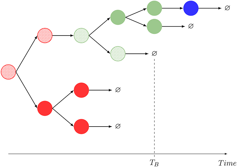
Figure 2. One realization of the stochastic process shown in Figure 1, and interpretation of the summary statistics. The dynamics mimics that of Hawkins et al. (35, Supplementary Material, Figure 2A) and Piltti et al. (36, Figure 2). In this example, M = 2, and a striped color identifies the original cell being tracked. A given color indicates the spatial location of each cell (red: blood, blue: C1, green: C2). In this realization, GB = 11, NB = NB(B) + NB(C1) + NB(C2) = 1 + 0 + 1 = 2. The compartment before death is C2.
Motivated by these experimental achievements, we introduce different stochastic descriptors (also known as summary statistics). Not all of them can be straightforwardly quantified but, interestingly, combined they give information about specific aspects of the cellular dynamics that are unattainable using standard population dynamics approaches. In particular, the process in Figure 2, similarly to that in Hawkins et al. (35, Supplementary Material, Figure 2A) or Piltti et al. (36, Figure 2), can be quantified in terms of the following statistics:
• Lifetime of a CD4+ T cell and number of division events of this cell during its lifetime,
for i ∈ {B, C1, …, CM}. If we define mi = 𝔼(Ti) and , one can show that
We note that although we only report here expressions for the mean values, the Laplace-Stieltjes transform of Ti, as well as the complete probability mass function of Ni, can be explicitly obtained.
• It is clear that the number of division events can be split as , where Ni(j) is the number of division events of a given cell taking place in the spatial compartment j ∈ {B, C1, …, CM}. The mean values (and the complete probability mass function, see section 1 in the Appendix) of these random variables Ni(j), , can also be analytically computed:
where 1A is a function equal to 1 if A is satisfied, and equal to 0 otherwise.
• One can identify the spatial compartment where the cell dies, in terms of the following probabilities
These probabilities are given by
• Finally, the summary statistics introduced above refer to a single cell, without keeping track of the daughters produced by cell division. To this end, one can analyse for a given original cell in Figure 1 its complete genealogy in terms of the random variable
and the mean values of these random variables, , can be computed as
For a particular realization of the stochastic process described by Figure 1, we show in Figure 2, the definition of this summary statistics.
We note that if on average, a larger number of division events take place than death ones, the corresponding branching process depicted in Figure 2 might explode. This means that, depending on the parameter values, one might have ℙ(Gi = +∞) > 0 and thus, 𝔼(Gi) = +∞. We find that sufficient conditions on the parameters to ensure ℙ(Gi = +∞) = 0, are given by
We also note that there is an intuitive interpretation of these conditions. In particular, for each spatial compartment Ci, the total rate of removing cells from this compartment (migration of cells, ξCi, B, or death, μCi) needs to be larger than the corresponding division rate λCi, so that cells do not indefinitely accumulate in this compartment. This is represented by Equation (1). On the other hand, it is not enough to export these cells to a different compartment if these cells cannot die sufficiently fast in a different compartment after they migrate, which is summarized by Equation (2), where blood acts as a special migration hub.
2.3. Fast-Migration Approximation
As we show in section 3 for CD4+ T cells in mice, the migration rates, {(ξB,Ci, ξCi, B), i ∈ {1, …, M}}, are of the order of min−1, and division, (λB, λC1, …, λCM), and death rates, (μB, μC1, …, μCM), are of the order of days−1. Thus, migration is several orders of magnitude faster. One can use this fact to propose a fast-migration approximation for the summary statistics above, and thus, to study a much simpler birth-and-death (or branching) process without spatial compartments.
We propose to approximate the journey of the cell under analysis, and its progeny, by considering a birth-and-death stochastic process within a single spatial compartment, with birth and death rates given by
where fj represents the fraction of time that the cell under study spends in each spatial compartment j ∈ {B, C1, …, CM}, in the absence of division and death (i.e., if only migration is considered in Figure 1). One could imagine that this birth-and-death process would approximate well the division and death dynamics of the original one when migration occurs at a much faster rate than division and death, so that steady state conditions (i.e., fi values) for the spatial location of the cell can be assumed before any division or death event occurs.
In order to compute the fraction fj, one needs to calculate the steady state probabilities for the process in Figure 1, in the absence of division and death, which satisfy the following system of equations
which leads to the solution
where we have introduced
Once this birth-and-death approximation has been introduced, one can propose the following simplifications:
• The average lifetime of the cell in the original model can be approximated by , which is its average lifetime in the fast-migration approximation, and does not depend on the initial compartment i. From now on, and when implementing the fast-migration approximation, we remove the initial compartment (labeled by i) in the notation.
• The average number of division events during the lifetime of a given cell in the original model can be approximated by , which is the average number of division events in the fast-migration approximation. Since , as explained in section 2.2, where N(j) is the number of division events in compartment j ∈ {B, C1, …, CM}, one can propose .
• The time for the progeny of a single cell to become extinct in the original process is not easy to analyse, and was not considered in section 2.2. Yet, it can be approximated by the time to extinction of a birth-and-death process with birth rate and death rate , for one single cell starting the process. This time follows a phase-type distribution (40), and its mean is given by (41).
• The probability of the original cell dying in compartment j ∈ {B, C1, …, CM} can be approximated by .
• The number of cells in the genealogy of a single cell in the original process can be approximated by the number of cells in the genealogy of a branching process with division rate and death rate . In particular, we can write (see section 1 in the Appendix for further details)
2.4. The Effect of Non-blood Mediated Migration
Thus far, we have considered that, as described in Figure 1, cells can only migrate from one compartment to another through blood. However, in Ganusov and Auerbach (3), the authors made a compelling case for direct migration between compartments, namely, non-mediated by blood. In this section, we make use of the same model as before, but allow for cells in compartment C1a to migrate directly to compartment C1b. The new scenario is described in Figure 3, where the dashed arrow is the new migration rate. Note that, following Ganusov and Auerbach (3), we do not allow for migration from C1a to blood.
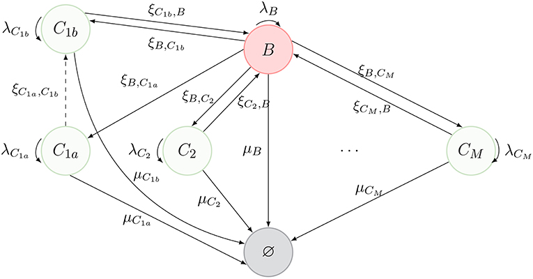
Figure 3. New process inspired by Ganusov and Auerbach (3, Figure 2), where T cells can migrate between two compartments (C1a and C1b) without transitioning through the blood.
In order to keep the notation consistent, we split the former compartment C1 into two compartments, labeled C1a and C1b, respectively. Thus, the process of Figure 1 represents the dynamics of Figure 3, when one is not interested in deciphering where exactly a given cell is located in C1 (i.e., if the cell is in C1a or C1b).
The summary statistics defined in section 2.2 could be analyzed for the process of Figure 3 in a similar way, but we do not present the details here. On the other hand, the fast-migration approximation can be implemented by considering the steady state migration dynamics of Figure 3, which leads to the new set of equations
One can solve this system of equations to find
Let us introduce
and , to be able to write
Interestingly, by adding the fractions in compartments C1a and C1b, we can map this model to the previous one if we define
and
We note that Equations (7)–(8) imply that the parameters (ξC1, B, ξB,C1) can be considered as effective migration rates between the blood and compartment C1, when C1 is merged from compartments C1a and C1b. The rate of a cell migrating from the blood to C1a or C1b, if one is not interested in where exactly it migrates to (i.e., migration to C1), would then be given by ξB,C1 = ξB,C1a + ξB,C1b [see Equation (7)]. On the other hand, for a cell in C1, the mean time to reach the blood () can be computed from the following analysis
Finally, Equation (8) can be derived by noting that
3. Numerical Results
In this section we carry out a numerical study to illustrate our analytical results and the fast-migration approximation, to compare our analytical results with those obtained from stochastic numerical simulations, and to show how dynamics occurring in a particular compartment can have a significant impact on the whole system. We propose in section 3.1 parameter values for the process described by Figure 1, based on those considered in den Braber et al. (1) and Ganusov and Auerbach (3). In section 3.2, we compare analytical and numerical results with those obtained from our fast-migration approximation. We analyse in section 3.3 the role played by the asymmetry in the death rates of the different spatial compartments. We focus in section 3.4 on the potential impact of (not blood-mediated) migration between compartments, inspired by the model considered in Ganusov and Auerbach (3).
3.1. Parameters
In Table 1, we provide baseline parameter values obtained from den Braber et al. (1) and Ganusov and Auerbach (3), for the model described in Figure 1 with M = 5. These spatial compartments represent, according to Ganusov and Auerbach (3), the blood (B), mesenteric lymph nodes and Peyer's patches (C1), lung (C2), liver (C3), spleen (C4) and subcutaneous lymph nodes (C5). In order to show the goodness of the fast-migration approximation, and to show the impact of spatial asymmetry in this system, we vary in section 3.2, section 3.3 and section 3.4 the division and death rates in the different spatial compartments, so that the values μ and λ in Table 1 should be considered baseline parameters for CD4+ T cells according to den Braber et al. (1).
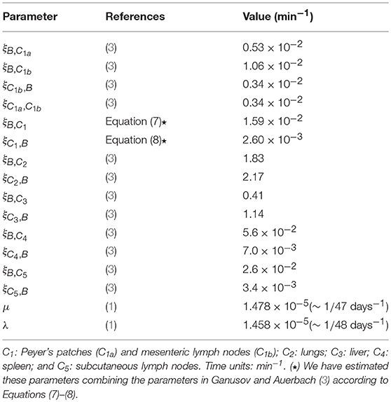
Table 1. Parameter values considered in the numerical study. Blood and M = 5 additional spatial compartments as in Ganusov and Auerbach (3, Figure 2).
We also note that the model in Ganusov and Auerbach (3) considers Peyer's patches and mesenteric lymph nodes as two different compartments (i.e., C1a and C1b, respectively, described in section 2.4). We propose in section 3.2 and section 3.3 to merge these compartments and analyse the cellular dynamics without deciphering where exactly a given cell in C1 is (i.e., if the cell is in the Peyer's patches or in the mesenteric lymph nodes), by using Equations (7)–(8) to obtain effective migration rates (ξB,C1, ξC1, B) in Table 1. In section 3.4 we carry out a numerical study of our second model, described in Figure 3, where the migration rates (ξB,C1a, ξB,C1b, ξC1b, B, ξC1a, C1b) are those in Ganusov and Auerbach (3). Finally, we note that for all the parameter values considered in this section, Equations (1)–(2) are satisfied.
3.2. Gillespie Simulations, Analytic Results, and Fast-Migration Approximation
In this section we set the migration rates {(ξB,Ci, ξCi, B), i ∈ {1, …, 5}} as given in Table 1. In order to show the goodness of the fast-migration approximation we set
for varying values of R > 0. We note that in the rest of the paper, but this section, we set R = 1. R = 1 corresponds to a completely symmetric scenario, where all compartments have death rate μ and division rate λ. For increasing values of R, the scenario becomes asymmetric, where division in the blood is less likely to occur compared to division in other compartments, while death rates are still the same in all spatial compartments. However, division and death rates for large values of R become comparable (similar order of magnitude) to migration rates.
In Figure 4, we plot (starting with a single cell in the blood) a) the mean number of division events in the blood and b) the mean number of division events in compartments {B, C1, C2}, as a function of log(R). The fast-migration (FM) approximation mostly provides reliable results when log(R) < 1.0. In this case, results obtained by simulations agree with the analytic results (obtained as detailed in section 2.2), and with the fast-migration approximation (computed as explained in section 2.3). We note that values log(R) < 1.0 correspond to division and apoptotic rates of the order of 10−5−10−4 min−1, and migration rates are of the order of 10−3−100 min−1. For log(R) > 1.0, division and death rates become comparable to some of the migration rates, and the fast-migration approximation provides results in Figure 4 which significantly differ from those obtained by numerical simulations and analytic methods. We also note that even for small values of log(R), other variables of interest cannot be well captured by the fast-migration approximation. This is the case for , the mean number of division events occurring in the blood for a cell starting in the blood. While the fast-migration approximation provides reliable results for log(R) = 0, once log(R) > 0 the true (analytic) value of fastly decays to zero. This behavior is captured by the stochastic simulations in Figure 4B, but not by the fast-migration approximation.
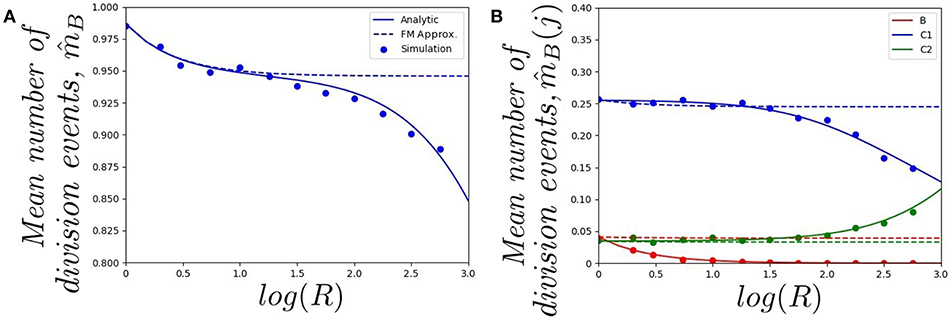
Figure 4. Effect of changing the value of R on (A) the mean total number of division events , and (B) the mean number of division events occurring in compartment j, , for j ∈ {B, C1, C2}. We consider a single cell starting in the blood. Analytic solution (solid), fast-migration approximation (dashed) and 104 stochastic simulations (dots).
In Figure 5, we plot a) the probability of the original cell dying in compartments {B, C1, C2}, and b) the mean total number of cells in the genealogy of the original cell, as a function of log(R) and for a cell starting in the blood. Similar comments to the ones above apply to the results in Figure 5A, where the fast-migration approximation behaves well for log(R) < 1.0. We also note that for small values of R we get βB(C1) > βB(B) > βB(C2) for the cell starting in the blood, which shows the importance of the migration dynamics in the fate of a given cell. However, the probability of the cell dying in the blood increases with increasing values of R as one would expect, since if division and death rates increase, the starting position of the cell has a larger impact on its proliferation and death dynamics and the impact of migration rates accordingly decreases. It is also interesting to note that the fast-migration approximation provides reliable results for all the values of R explored in Figure 5B. In this case, we study the mean number of cells in the genealogy, which is a population-based descriptor rather than a descriptor only related to a given cell. This result is striking, since division and death rates for log(R) > 2.0 are of the order of 10−3−10−2 min−1, which are comparable to the migration rates in Table 1. This might indicate that the fast-migration approximation could behave better when dealing with population-based summary statistics, while it is reliable when analysing single cell descriptors only for small enough values of the division and death rates (compared to migration rates).
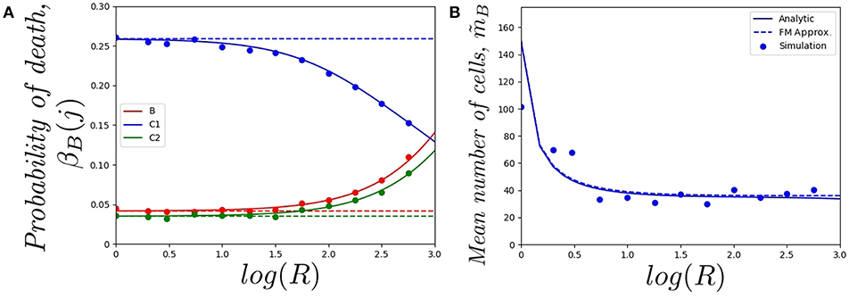
Figure 5. Effect of changing the value of R on (A) the probability of the cell dying in compartment j, for j ∈ {B, C1, C2}, and (B) the mean total number of cells in the genealogy of the original cell, . We consider a single cell starting in the blood. Analytic result (solid), fast-migration approximation (dashed) and 104, for (A), and 103, for (B), stochastic simulations (dots).
It is also worth noting that simulating stochastic processes with different timescales is a challenging problem from a computational point of view, which in our case means simulating the migration of cells (timescales of the order of minutes), until some division or death events occur (in days). This is even more challenging when dealing with a population of cells (see Figure 5B) rather than a single cell (Figures 4, 5A). For these computational reasons, 103 stochastic simulations were used to compute the values in Figure 5B, compared to 104 simulations for Figures 4, 5A. Thus, our results in Figure 5B illustrate the need for developing the analytical results of section 2.2, or related approximations, such as the one in section 2.3, instead of using standard stochastic simulations to analyse cellular dynamics in these systems.
3.3. The Role of Different Death Rates in Different Compartments
We have assumed that death rates are the same in all compartments. However, taking into account that migration rates determine the relative weight of each compartment in the overall behavior of the system, in this section we analyse the role of different death rates in compartments C1 (where migration from blood is around six times faster than the reverse) and C3 (where migration from blood is around one third slower than the reverse) (3).
Figure 6A shows the impact of varying the death rate μC1 in compartment C1 (with respect to the one in Table 1 μC1 = μ, shown as a vertical solid line). It is interesting to note how compartment C4 is one of the most sensitive to this parameter in spite of the fact that we are only changing the death rate of compartment C1. The rationale behind this result is related to the relative immigration to emigration rates in each compartment. In particular, using the migration rates of Table 1 we find K1 = 6.115, K2 = 0.843, K3 = 0.360, K4 = 8.000, K5 = 7.647 (namely, immigration in C1 is 6.115 times larger than emigration). The three compartments with higher immigration/emigration ratios are C1, C4 and C5. Thus, when μC1 increases, the weight of the dynamics is shifted to the compartment with the highest such ratio. On the other hand, in Figure 6B, as compartment C3 has low K3 = 0.360, the most sensitive probability of death with respect to parameter μC3 is βB(C3).
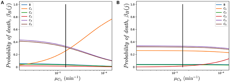
Figure 6. Effect of varying μCi on the probability βB(j) of dying in different compartments j ∈ {B, C1, …, C5}, for a cell starting at blood. (A) Varying μC1; (B) Varying μC3. The vertical black line represents the value μ.
Similarly, Figure 7A shows the effect of changing μC1 on the mean lifetime of a cell. Again, the role of Ki is very relevant. While in both cases (changing μC1 or μC3) the mean lifetime decreases (as expected), the effect is milder in the case of μC3. This is related to the fact that, due to the reduced immigration rate into compartment C3, the odds of finding the cell in that compartment are relatively low. On the contrary, as the cell spends more time in compartment C1, varying the death rate in that compartment increases/decreases quickly the mean lifetime when the death rate decreases/increases, respectively.
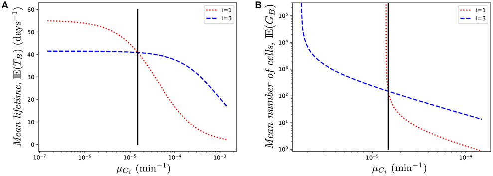
Figure 7. Effect of changing the value of one death rate, μCi on (A) the mean lifetime, E(TB), and (B) the mean number of cells in the genealogy, E(GB), for a cell starting at blood. The vertical black line represents the value μ.
Finally, in Figure 7B we show the mean number of cells produced by a single cell during its lifetime (the size of the offspring tree). Again, in the case of compartment C1, reducing slightly the death rate produces a transition from finite to infinite number of descendants, which is directly related to the conditions given by Equations (1)–(2), and relates to the asymptotic behavior observed in Figure 7B. In this case, small changes in the parameters might have a huge impact on the cell population dynamics.
Overall, these analyses show that, not only migration rates, but the ratio between immigration and emigration rates affect the overall dynamics of the system. Thus, analysing these ratios, and their interplay with the apoptotic and proliferation rates, can help to identify the most relevant locations of the immune system related to the fate of a single cell.
3.4. The Role of Direct Migration Between Compartments
To test the relevance of migration between compartments (as emphasized in Ganusov and Auerbach (3)) we compute the fractions, fB, fC1a, …, fC5 using the parameters from Table 1. We have
where, as we defined above, fj represents the fraction of time that the cell under study spends in each spatial compartment j ∈ {B, C1, …, CM}, in the absence of division and death. Furthermore, in Figure 8 we show the dependence of these fractions on the rate connecting compartments C1a and C1b, ξC1a, C1b. Clearly, as ξC1a, C1b → 0, compartment C1a becomes a sink of cells so that fC1a → 1 and the rest tend to 0.
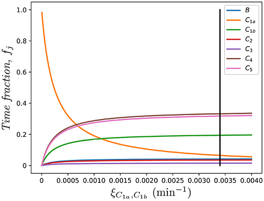
Figure 8. Effect of the migration rate ξC1a, C1b on the fraction of time spent in each compartment, fj, for j ∈ {B, C1a, C1b, C2, …, C5}. The vertical black line represents the value ξC1a, C1b in Table 1, as in Ganusov and Auerbach (3).
3.5. Sensitivity Analysis
For the original model in Figure 1, we can use Equation (3) to compute the sensitivity matrix S. Using the parameters in Table 1, we find that the matrix S is given by
where the rows stand for fB, fC1, …, fC5 and the columns for ξB,C1, ξC1, B, …, ξC5, B. That is, matrix S is defined so that
While this matrix is informative, it does not reflect a property of Equation (3); namely, that the relevant quantities are not migration rates themselves but, rather, the immigration/emigration ratio for each spatial compartment. Thus, one can obtain a simpler version of the sensitivity matrix with respect to the ratios Ki, i ∈ {1, …, 5}:
where each row corresponds to a given fraction, fj, and with the columns representing (K1, K2, K3, K4, K5), where K1 = 6.115, K2 = 0.843, K3 = 0.360, K4 = 8.000, K5 = 7.647, so that
Due to some symmetries in Equation (3) with respect to Ki, the reduced sensitivity matrix has many repeated entries. Biologically, this is a remarkable result as it shows that events occurring in different compartments can affect equally a given one. Another conclusion can be derived from the sign of the elements of . These signs can be easily understood by noting that, since Ki represents the fraction of immigration to emigration events in a given compartment, the higher Ki the higher the probability of finding a cell in compartment Ci.
4. Discussion and Conclusions
We propose a mathematical model for the migration, proliferation and death of a CD4+ T cell, and focus on a number of observables which refer to the single cell journey during its lifetime, as well as to the dynamics of its progeny. We have presented analytical methods to study these observables and have provided conditions for this cellular system not to explode. A fast-migration approximation can be proposed when migration events occur significantly faster than division and death, so that steady state conditions can be assumed for the spatial location of the cell.
Our numerical results show that most of the stochastic observables under study can be properly captured by means of the fast-migration approximation, when migration rates are (at least) one order of magnitude larger than division and death rates. The fast-migration approximation is able to appropriately capture the mean number of cells in the genealogy of a given cell, even when migration events occur at a similar rate to those of division and death events. It is also worth mentioning that our numerical results illustrate how perturbing a single rate in a given spatial compartment can have a significant impact on the cellular dynamics and observables corresponding to other compartments, which indicates the clear interplay between cellular dynamics in the different spatial compartments, and which depends on the specific migration structure (and rates) of the system. Finally, a particular feature of our analytical approach is that it allows for an exact sensitivity analysis of each of the observables with respect to each kinetic rate. In this way the contribution that each particular rate (i.e., event) has on a given stochastic observable can be assessed.
Recent experimental advances allow us to observe biological processes at the single cell level, but at the same time these new experimental techniques are still far from being able to provide a full picture of migration, division and death events in vivo. Thus, experimental observations need to be combined with mathematical and computational models which allow one to test hypotheses, shed some light on cellular dynamics or to design new or different experiments. As a consequence, two main challenges that directly arise are: (i) to develop new analytical techniques to study different observables in these cellular systems, which can be compared to experimental measurements, and (ii) to propose new and more advanced methodologies for calibrating these mathematical models by using experimental data. Although our focus in this work is on (i), our results can have a direct impact on (ii), since the distributions and mean values computed in section 2 could be used to calculate the likelihood function when applying Bayesian statistical methods for parameter estimation and model calibration.
Finally, it is worth noting that, unlike population dynamics models (based on collective counts of cells), our stochastic descriptors have two clear advantages. First of all, they represent variables directly related to the dynamics of a single cell, and thus, allow us to bridge between the novel experimental techniques described in section 2.2 and specific proliferation, death or migration rates at the cell level. Secondly, our descriptors allow us to quantify these individual rates. For instance, in practice only the net division rate can be measured but, combining descriptors, we can separate birth from death or migration rates. Naturally, these estimates require the use of both more sophisticated experiments and parameter estimation techniques (such as the Bayesian methods mentioned above).
Author Contributions
ML-G, MC, and GL designed and analyzed the summary statistics and the fast-migration approximation. ML-G, MC, NA, and LdlH wrote the numerical codes and performed the numerical simulations. ML-G, MC, LdlH, GL, and CM-P contributed to writing the manuscript. All authors contributed to the development of the mathematical model and reviewing the literature and to revising the manuscript.
Funding
This work has been supported by Arthritis Research UK A25929 and Cancer Research UK C62155 (CM-P). This work has been also partially supported by grant FIS2016-78883-C2-2-P (Ministerio de Economia, Industria y Competitividad - Agencia Estatal de Investigacion) and PRX 16/00287 (MC), PIRSES-GA-2012-317893 (MC, ML-G, GL and CM-P), PITN-GA-2012-317040 (LdlH, GL, and CM-P), the European Union H2020 Programme under agreement 764698 MSCA-ITN-2017, QuanTII ETN (GL and CM-P), and the Spanish Ministry of Economy and Competitiveness MTM2014-58091-P (ML-G).
Conflict of Interest Statement
The authors declare that the research was conducted in the absence of any commercial or financial relationships that could be construed as a potential conflict of interest.
Supplementary Material
The Supplementary Material for this article can be found online at: https://www.frontiersin.org/articles/10.3389/fimmu.2019.00194/full#supplementary-material
References
1. den Braber I, Mugwagwa T, Vrisekoop N, Westera L, Mögling R, de Boer AB, et al. Maintenance of peripheral naive T cells is sustained by thymus output in mice but not humans. Immunity. (2012) 36:288–97. doi: 10.1016/j.immuni.2012.02.006
2. Thome JJ, Yudanin N, Ohmura Y, Kubota M, Grinshpun B, Sathaliyawala T, et al. Spatial map of human T cell compartmentalization and maintenance over decades of life. Cell. (2014) 159:814–28. doi: 10.1016/j.cell.2014.10.026
3. Ganusov VV, Auerbach J. Mathematical modeling reveals kinetics of lymphocyte recirculation in the whole organism. PLoS Comput Biol. (2014) 10:e1003586. doi: 10.1371/journal.pcbi.1003586
4. Herzenberg LA, Parks D, Sahaf B, Perez O, Roederer M, Herzenberg LA. The history and future of the fluorescence activated cell sorter and flow cytometry: a view from Stanford. Clin Chem. (2002) 48:1819–27. Available online at: http://clinchem.aaccjnls.org/content/clinchem/48/10/1819.full.pdf
5. Johnson J, Nowicki MO, Lee CH, Chiocca EA, Viapiano MS, Lawler SE, et al. Quantitative analysis of complex glioma cell migration on electrospun polycaprolactone using time-lapse microscopy. Tiss Eng C Methods. (2009) 15:531–40. doi: 10.1089/ten.tec.2008.0486
6. Westera L, Drylewicz J, Den Braber I, Mugwagwa T, Van Der Maas I, Kwast L, et al. Closing the gap between T-cell life span estimates from stable isotope-labeling studies in mice and humans. Blood. (2013) 122:2205–12. doi: 10.1182/blood-2013-03-488411
7. Gosling JP, Krishnan SM, Lythe G, Chain B, MacKay C, Molina-París C. A mathematical study of CD8+ T cell responses calibrated with human data. arXiv preprint arXiv:180205094 (2018).
8. Seddon B, Yates AJ. The natural history of naive T cells from birth to maturity. Immunol Rev. (2018) 285:218–32. doi: 10.1111/imr.12694
9. Mason D. A very high level of crossreactivity is an essential feature of the T-cell receptor. Immunol Tod. (1998) 19:395–404. doi: 10.1016/S0167-5699(98)01299-7
10. Jenkins MK, Chu HH, McLachlan JB, Moon JJ. On the composition of the preimmune repertoire of T cells specific for peptide-major histocompatibility complex ligands. Ann Rev Immunol. (2010) 28:275–94. doi: 10.1146/annurev-immunol-030409-101253
11. Itano AA, Jenkins MK. Antigen presentation to naive CD4 T cells in the lymph node. Nature Immunol. (2003) 4:733–9. doi: 10.1038/ni957
12. Sallusto F, Lenig D, Förster R, Lipp M, Lanzavecchia A. Two subsets of memory T lymphocytes with distinct homing potentials and effector functions. Nature. (1999) 402:34–8. doi: 10.1038/35005534
13. Masopust D, Schenkel JM. The integration of T cell migration, differentiation and function. Nat Rev. Immunol. (2013) 13:309–20. doi: 10.1038/nri3442
14. Farber DL, Yudanin NA, Restifo NP. Human memory T cells: generation, compartmentalization and homeostasis. Nat Rev Immunol. (2014) 14:24. doi: 10.1038/nri3567
15. Kumar BV, Connors TJ, Farber DL. Human T cell development, localization, and function throughout life. Immunity. (2018) 48:202–13. doi: 10.1016/j.immuni.2018.01.007
16. Davis MM, Brodin P. Rebooting human immunology. Ann Rev Immunol. (2018) 36:843–64. doi: 10.1146/annurev-immunol-042617-053206
17. Blum KS, Pabst R. Lymphocyte numbers and subsets in the human blood: do they mirror the situation in all organs? Immunol Lett. (2007) 108:45–51. doi: 10.1016/j.imlet.2006.10.009
18. Ganusov VV, De Boer RJ. Do most lymphocytes in humans really reside in the gut? Trends Immunol. (2007) 28:514–8. doi: 10.1016/j.it.2007.08.009
19. Hogan T, Gossel G, Yates AJ, Seddon B. Temporal fate mapping reveals age-linked heterogeneity in naive T lymphocytes in mice. Proc Natl Acad Sci USA. (2015) 112:E6917–26. doi: 10.1073/pnas.1517246112
20. Gonçalves P, Ferrarini M, Molina-Paris C, Lythe G, Vasseur F, Lim A, et al. A new mechanism shapes the naïve CD8+ T cell repertoire: the selection for full diversity. Mol Immunol. (2017) 85:66–80. doi: 10.1016/j.molimm.2017.01.026
21. Baliu-Piqué M, Kurniawan H, Ravesloot L, Verheij M, Drylewicz J, Lievaart-Peterson K, et al. Age-related distribution and dynamics of T cells in blood and lymphoid tissues of goats. Dev Comp Immunol. (2018) 93:1–10. doi: 10.1016/j.dci.2018.12.004
22. Knabel M, Franz TJ, Schiemann M, Wulf A, Villmow B, Schmidt B, et al. Reversible MHC multimer staining for functional isolation of T-cell populations and effective adoptive transfer. Nat Med. (2002) 8:631. doi: 10.1038/nm0602-631
23. Krutzik PO, Nolan GP. Fluorescent cell barcoding in flow cytometry allows high-throughput drug screening and signaling profiling. Nat Methods. (2006) 3:361. doi: 10.1038/nmeth872
24. Schwab SR, Cyster JG. Finding a way out: lymphocyte egress from lymphoid organs. Nat Immunol. (2007) 8:1295. doi: 10.1038/ni1545
25. Westermann J, Söllner S, Ehlers EM, Nohroudi K, Blessenohl M, Kalies K. Analyzing the migration of labeled T cells in vivo: an essential approach with challenging features. Lab Invest. (2003) 83:459. doi: 10.1097/01.LAB.0000062852.80567.90
26. Pham K, Shimoni R, Charnley M, Ludford-Menting MJ, Hawkins ED, Ramsbottom K, et al. Asymmetric cell division during T cell development controls downstream fate. J Cell Biol. (2015) 210:933–50. doi: 10.1083/jcb.201502053
27. Sawicka M, Stritesky G, Reynolds J, Abourashchi N, Lythe G, Molina-París C, et al. From pre-DP, post-DP, SP4, and SP8 thymocyte cell counts to a dynamical model of cortical and medullary selection. Front Immunol. (2014) 5:19. doi: 10.3389/fimmu.2014.00019
28. Artalejo J, Gómez-Corral A, López-García M, Molina-París C. Stochastic descriptors to study the fate and potential of naive T cell clonotypes in the periphery. J Math Biol. (2017) 74:673–708. doi: 10.1007/s00285-016-1020-6
29. Reynolds J, Coles M, Lythe G, Molina-París C. Deterministic and stochastic naïve T cell population dynamics: symmetric and asymmetric cell division. Dyn Syst. (2012) 27:75–103. doi: 10.1080/14689367.2011.645447
30. Donovan GM, Lythe G. T-cell movement on the reticular network. J Theor Biol. (2012) 295:59–67. doi: 10.1016/j.jtbi.2011.11.001
31. Currie J, Castro M, Lythe G, Palmer E, Molina-París C. A stochastic T cell response criterion. J R Soc Interface. (2012) 9:2856–70. doi: 10.1098/rsif.2012.0205
32. Huth J, Buchholz M, Kraus JM, Mølhave K, Gradinaru C, Wichert Gv, et al. TimeLapseAnalyzer: multi-target analysis for live-cell imaging and time-lapse microscopy. Comput Methods Progr Biomed. (2011) 104:227–34. doi: 10.1016/j.cmpb.2011.06.002
33. Klein J, Leupold S, Biegler I, Biedendieck R, Münch R, Jahn D. TLM-Tracker: software for cell segmentation, tracking and lineage analysis in time-lapse microscopy movies. Bioinformatics. (2012) 28:2276–7. doi: 10.1093/bioinformatics/bts424
34. Hilsenbeck O, Schwarzfischer M, Skylaki S, Schauberger B, Hoppe PS, Loeffler D, et al. Software tools for single-cell tracking and quantification of cellular and molecular properties. Nat Biotechnol. (2016) 34:703. doi: 10.1038/nbt.3626
35. Hawkins E, Markham J, McGuinness L, Hodgkin P. A single-cell pedigree analysis of alternative stochastic lymphocyte fates. Proc Natl Acad Sci USA. (2009) 106:13457–62. doi: 10.1073/pnas.0905629106
36. Piltti KM, Cummings BJ, Carta K, Manughian-Peter A, Worne CL, Singh K, et al. Live-cell time-lapse imaging and single-cell tracking of in vitro cultured neural stem cells–Tools for analyzing dynamics of cell cycle, migration, and lineage selection. Methods. (2018) 133:81–90. doi: 10.1016/j.ymeth.2017.10.003
37. Reinhardt RL, Khoruts A, Merica R, Zell T, Jenkins MK. Visualizing the generation of memory CD4 T cells in the whole body. Nature. (2001) 410:101. doi: 10.1038/35065111
38. Masopust D, Vezys V, Marzo AL, Lefrançois L. Preferential localization of effector memory cells in nonlymphoid tissue. Science. (2001) 291:2413–7. doi: 10.1126/science.1058867
39. Sathaliyawala T, Kubota M, Yudanin N, Turner D, Camp P, Thome JJ, et al. Distribution and compartmentalization of human circulating and tissue-resident memory T cell subsets. Immunity. (2013) 38:187–97. doi: 10.1016/j.immuni.2012.09.020
Keywords: T cell, stochastic model, continuous-time Markov chain, single cell, cellular fate, migration, division, apoptosis
Citation: de la Higuera L, López-García M, Castro M, Abourashchi N, Lythe G and Molina-Paris C (2019) Fate of a Naive T Cell: A Stochastic Journey. Front. Immunol. 10:194. doi: 10.3389/fimmu.2019.00194
Received: 28 June 2018; Accepted: 23 January 2019;
Published: 06 March 2019.
Edited by:
Jorge Bernardino De La Serna, United Kingdom Research and Innovation, United KingdomReviewed by:
Ruian Ke, Los Alamos National Laboratory (DOE), United StatesM. J. Lopez-Herrero, Complutense University of Madrid, Spain
Maria Teresa Rodrguez Bernal, Universidad Complutense de Madrid, Spain
Copyright © 2019 de la Higuera, López-García, Castro, Abourashchi, Lythe and Molina-Paris. This is an open-access article distributed under the terms of the Creative Commons Attribution License (CC BY). The use, distribution or reproduction in other forums is permitted, provided the original author(s) and the copyright owner(s) are credited and that the original publication in this journal is cited, in accordance with accepted academic practice. No use, distribution or reproduction is permitted which does not comply with these terms.
*Correspondence: Martín López-García, m.lopezgarcia@leeds.ac.uk
†These authors have contributed equally to this work