Wave exposure as a predictor of benthic habitat distribution on high energy temperate reefs

Introduction

A major difficulty faced by managers in developing policy and implementing measures to safeguard ecologically important areas of the oceans is the relative paucity of scientific information available to direct and inform such initiatives. In comparison to terrestrial ecosystems, spatial management of marine ecosystems has been constrained by the lack of high quality, spatially explicit data describing the basic patterns of their biophysical constituents. This is for the most part a function of the inherent difficulties and costs associated with data collection in the marine environment. As a result quantitative spatial information in marine ecosystems is typically sparse, localized and patchily distributed through space and time (Kostylev and Hannah, 2007; Foster et al., 2009).

The emergence of remotely sensed acoustic technologies coupled with the ability to collect seabed information with georeferenced towed camera systems, opens the possibility of surveying large areas of seafloor and producing high resolution maps of topography, subsurface structures, and benthic habitats (Rattray et al., 2009). Acoustic habitat mapping utilizes sonar-derived physical variables as proxies to describe the range of abiotic conditions (e.g., substrate type) and processes (e.g., light availability) that define the realized niche and subsequent distribution of benthic species and assemblages. Commonly, features used to predict the distribution of benthic assemblages are derived directly from topographic information and acoustic backscatter response. Thus, the role of wave exposure on habitat distribution is only indirectly considered through postulated associations with water depth and seafloor orientation (aspect). Wave energy, however, varies spatially and temporally, and is locally modified by factors such as coastline geometry and bottom topography. It is therefore unlikely in shallow coastal zones that depth and orientation of an area of the seafloor are fully indicative of structuring effects of exposure on biological assemblages, especially in areas which are known to experience gradients in wave activity.

The southern Australian coastline is one of the highest energy coastlines in the world (Hemer et al., 2008; Hughes and Heap, 2010). As a result, wave energy is arguably one of the primary variables influencing the morphology, community structure and spatial organization of benthic taxa in the region (Wernberg and Goldberg, 2008; Wernberg and Vanderklift, 2010). The effects of wave energy on the composition, functional morphology and distribution of species and assemblages have been documented in most areas of the shallow marine environment across a wide range of taxonomic groups. The hydrodynamic energy regime has been demonstrated as an important factor controlling the spatial distribution of macroalgae (Pedersen et al., 2012; Thomson et al., 2012), sessile invertebrates (Bell and Barnes, 2000; Chollett and Mumby, 2012), seagrasses (Fonseca and Bell, 1998; Turner et al., 1999), mollusks (Boulding et al., 1999; Pfaff et al., 2011) and fishes (Letourneur, 1996; Friedlander et al., 2003), and has been identified as a key indicator of species abundance and diversity (Denny, 2006).

Wave energy determines benthic habitat availability through a number of direct and indirect processes which exert effects on benthic organisms (Denny, 2006). Sessile benthic taxa are reliant on water circulation for delivery of nutrients and oxygen, timing and dispersal of larvae and propagules, and removal of waste. Hydrodynamic exposure is also an important agent of stress and disturbance through sediment flux processes, specifically abrasion, burial and limitation of light availability (Airoldi, 2003), or mechanical tearing or removal of sessile species from their places of attachment (Thomsen et al., 2004). On shallow rocky reefs dominated by canopy forming kelps, wave energy may also determine canopy size, morphology and spatial patchiness, influencing understory community composition through altering light availability, water motion and direct physical abrasion (Toohey et al., 2004).

There are relatively few studies that use a direct proxy of hydrodynamic exposure as a variable for predictive mapping. Quantitative estimation by cartographic fetch models or more complex mathematical simulations of sea state have been used to derive exposure/organism relationships and also to predict their distributional patterns (Bekkby et al., 2008). At the local scale, cartographic fetch models based on the distance from a given location over which wind waves are able to generate (i.e., distance to barrier) have also been used to quantify a metric of exposure often assigned to a fixed number of ordinal categories (Lindegarth and Gamfeldt, 2005). Fetch-based exposure models have been demonstrated to respond well in enclosed or semi-enclosed areas where coastal perturbations, inlets or islands are the principal mediators of local wave energy (Ekebom et al., 2003; Greenlaw et al., 2011), but are potentially less applicable to open coasts where submarine topography such as offshore banks or reefs are often the significant factors mediating fully-developed wave conditions from remote synoptic events (Chollett and Mumby, 2012). Numerical wave modeling approaches are commonly used in coastal engineering applications and are capable of incorporating the combined effects of complex seabed topography and coastlines as well as spatial variation in wave energy caused by shallow water processes such as refraction, diffraction, wave on wave interactions and energy dissipation due to white-capping and wave breaking. Their use in local-scale ecological studies however has not been widely reported (England et al., 2008). This is potentially due to the computational complexity and expert knowledge required for their implementation (Hill et al., 2010).

While sonar methods have been well demonstrated to provide useful proxies of the relatively static geophysical patterns that reflect distribution of benthic species and assemblages, the spatially and temporally variable influence of hydrodynamic energy on benthic habitat distribution has been less well studied. Given the strong associations between marine taxa and their hydrodynamic environment, it is expected that measures of wave energy will also provide useful information for benthic habitat characterization and mapping. The principal hypothesis under investigation in this study is that a surrogate measure of wave energy can be used to improve the predictive accuracy of acoustic mapping techniques for sublittoral benthic habitat characterization. We investigate the effectiveness of a proxy for wave energy by comparing classified maps and measures of variable importance derived using predictors of depth and seafloor morphology, to those derived inclusive of a model of wave-induced orbital velocity.

Materials and Methods

Study Area

The study was conducted on the Otway coast of Victoria, south-eastern Australia. The site extends ~95 km from east to west around Cape Otway, the prominent coastal feature of western Victoria (Figure 1). Acoustic data for the site were acquired in four survey blocks of approximately equal area using a Reson Seabat 101 multibeam echosounder (MBES) operating at a frequency of 240 kHz aboard the Australian Maritime College vessel R.V. Bluefin. Block 1 was surveyed in November 2005 and blocks 2–4 in November 2007. Together, the four survey blocks encompass 624 km² of seafloor ranging in depth from 8 to 79 m. Large sandy embayments characterize the site with topographically complex rocky reef systems extending offshore from major headlands. Areas of shallow reef (10–30 m) were populated by diverse assemblages of macroalgae which are characterized by the canopy forming kelps Phyllospora comosa and Ecklonia radiata, while deeper reefs were populated by diverse communities of sponges and other sessile invertebrates.

FIGURE 1

Figure 1. Location and depth structure of the 624 km² study site at Cape Otway south-eastern Australia superimposed with hill-shaded MBES bathymetry. Numerals (1–4) represent each of the four MBES survey blocks (outlined in blue) undertaken at the site. Letters (A–E) identify major reef systems that are referred to throughout the study. Representative contiguous reef systems (B, D, and E) are shown in detail panels. Black lines indicate recorded path of acoustically-positioned towed video transects undertaken in February 2006 (Block 1) and February 2008 (Blocks 3–4).

The wave climate at the site, like much of the continental margin of southern Australia, is largely dominated by swell waves propagating from west to east moving low pressure systems in the Southern Ocean (Hemer et al., 2008). The majority of Australia's southern shelf is subject to persistent high energy swells of above 3.5 m 30–50% of the time (Porter-Smith et al., 2004) and annual return significant wave heights of up to 8.7 m (Harris and Hughes, 2012). The orientation of Cape Otway to prevailing swells originating from the south-west quadrant causes a gradient of wave energy across the site from highly exposed on the western side to moderately exposed in the east.

MBES Data Acquisition and Processing

Prior to each survey, calibration offsets for pitch, roll, yaw and latency were applied after conducting a detailed patch test. Daily sound velocity profiles were collected at the deepest area of the site during survey period to correct for local variations in sound velocity through the water column during processing. Positioning was accomplished using a real-time differential GPS integrated with a positioning and orientation system for marine vessels (POS MV) for dynamic heave, pitch, roll and yaw corrections (± 0.1° accuracy). Navigation, data logging, real-time quality control and display were carried out using Starfix suite 7.1 (Fugro proprietary software). The sounding data were edited on board ship and corrections for tides, sound velocity, vessel draft, settlement, squat and relative position of the transducer head were applied. The raw xyz data were then used to produce a bathymetric grid at 2.5 m horizontal resolution and a range resolution of ±12.5 mm. Backscatter values were corrected for gain and time varied gain using the University of New Brunswick (UNB1) algorithm (Starfix suite 7.1). Backscatter processing also corrected for transmission loss, the actual area of ensonification on the bathymetric surface, source level, and transmit and receive beam patterns. Additionally backscatter was corrected for seafloor bathymetric slope derived from the MBES bathymetry dataset. This resulted in normalized corrected grid (2.5 m resolution) representing relative backscatter intensity (dB).

Processed bathymetry and backscatter grids from each of the 4 survey blocks were combined at their highest resolution of 2.5 m. Edges between each of the survey blocks were normalized whereby overlapping values at a distance of 50 pixels (250 m on ground) from the edge of each block were averaged using a linear ramping technique. In order to minimize misregistration error between MBES products and in situ video observations, bathymetry and backscatter images for the entire site were resampled to a resolution of 5 m cell size before further processing.

A suite of environmental data was derived from the MBES datasets using a variety of neighborhood based topographic and spectral methods (see Rattray et al., 2013 for further information regarding derivative products). Prior to analysis, multi-collinearity of derivative variables was assessed using a step-wise procedure where at each iteration the variable with the greatest variance inflation factor (VIF) was removed until remaining covariates displayed VIF values less than 10. MBES bathymetry, backscatter and retained derivatives were geographically overlaid to form an image stack of 12 predictor variables (Table 1). Further to the previously described set of MBES-derived predictor variables, a model representing energy exposure at the seabed was developed.

TABLE 1

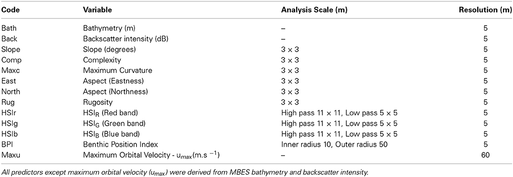
Table 1. Environmental predictor variables used to inform the Random Forests models.

Wave Energy Model

A fine-scale (60 m cell size) estimation of wave-induced orbital velocities at the seabed, used here as a surrogate for wave exposure, was created using a 3 step process:

(1) Results of a global wave hindcast model were downscaled to a regional scale (Victorian coastline) spectral wave model.

(2) A Detailed spectral wave model of the Otway coastline (study area) was created by incorporating local bathymetric variation (MBES and LIDAR derived). The wave boundaries for the detailed spectral wave model were downscaled from the regional wave model based on 1 year of representative annual wave conditions derived from a longer term wave climate assessment undertaken with the regional wave model.

(3) Wave-induced orbital velocities were transferred to the seabed by applying linear wave theory to surface spectral wave conditions.

Regional-scale model parameterization

Numerical wave modeling was accomplished using a MIKE 21 spectral wave (SW) model developed by Water Technology Pty Ltd using the DHI MIKE software suite (DHI, 2012¹) applied to a bathymetry mesh generated from the LIDAR / Multibeam mosaic and boundary depths derived from the Geoscience Australia 2009 bathymetry grid (0.025°) (Whiteway, 2009). MIKE 21 SW is a 3rd generation spectral wind-wave model capable of simulating wave growth by action of wind, non-linear wave-wave interaction, dissipation by white-capping, dissipation by wave breaking, dissipation due to bottom friction, refraction due to depth variations, and wave-current interaction. The model domain incorporated the western and eastern coastlines of Victoria, Tasmania and adjacent areas of continental shelf including Bass Strait (Figure 2). Long-term directional distribution and size of significant wave heights from the Wavewatch 3 model between the years 2000 and 2010 were obtained for the region. We compared the directional distribution and magnitude of significant wave heights for each year against the 10-year average, and selected the year that displayed the most similarities to the long-term record. Annual variability in significant wave heights and mean wave direction was generally low across the 10-year period. The year 2000 was selected as it contained the fewest extreme values (outliers) with respect to the 10-year average (Figure 3). Global hindcast results (10 m u and v wind velocity) from the National Oceanic and Atmospheric Administration (NOAA) Wavewatch 3 model were extracted and linearly interpolated (0.25° spatial, 3-hourly temporal) to provide boundary inputs for the regional scale spectral wave model. Spatially and temporally varying open wave results from the NOAA model provided wave boundary conditions along the western, southern and eastern model boundaries.

FIGURE 2

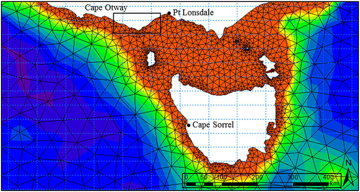
Figure 2. Domain of the regional spectral wave model incorporating the eastern and western coastlines of Victoria, Tasmania and Bass Strait. The triangular irregular network used to inform the numerical wave model was created from the 0.0025° Australian national bathymetry grid. Boundary inputs were obtained from the NOAA Wavewatch III global hindcast model. Wave buoy locations used to calibrate the model are located at Point Lonsdale (Victoria) and Cape Sorell (Tasmania). Extents of study area (Figure 1) are shown in box.

FIGURE 3

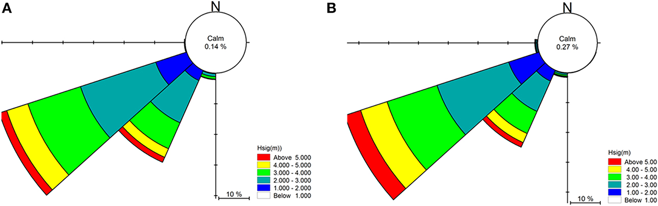
Figure 3. Summary of significant wave heights (Hsig), direction and percentage occurrence for Cape Otway showing prevailing swell conditions for (A) the year 2000 and (B) the 10-year average (2000–2010).

The regional spectral wave model was calibrated and validated against measured wave buoy data from Cape Sorell on the west coast of Tasmania (42° 7.2′S 145°E) and Point Lonsdale, south west of Melbourne (38° 18.2′S 144° 34.2′E) for the year 2000. Comparative agreement of hindcast wave conditions (significant wave height and peak period) to measured data was considered appropriate to use this model to assess wave climate along the Victorian coastline.

Local-scale model parameterization

A site-specific spectral wave model was generated for the waters around Cape Otway with western, southern and eastern boundary conditions provided by the regional scale model (Figure 4). A spectral wave hindcast was generated using a combination of the 0.0025° bathymetry grid, local MBES bathymetry (5 m) and bathymetric LIDAR (5 m) (Zavalas et al., 2014) to provide depth attenuation inputs in order to accurately propagate waves to uppermost extent of the sublittoral zone.

FIGURE 4

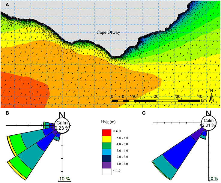
Figure 4. Local scale spectral wave model hindcast for the year 2000 for the Cape Otway coast, Victoria, Australia (A). Depth attenuation information was provided using MBES (5 m) and LiDAR (5 m) bathymetry, while boundary conditions were obtained from the regional spectral wave model (Figure 2). Summaries of significant wave height (Hsig) and direction under typical prevailing south westerly swell conditions for (B) west and (C) east of the southernmost point of Cape Otway.

Modeled wave conditions corresponding to significant wave height and spectral peak period for the year were used to calculate a spatially explicit estimate of maximum instantaneous bottom orbital velocity (u_max), used here as a surrogate for exposure to wave-induced energy. Linear wave theory was then used to predict the horizontal component of the wave orbital velocity (u_o) at a particular area on the seabed for small-amplitude, monochromatic waves as follows:

$u_o=\left[\frac{H\pi }{Tsinh(kd)}\right]·\text{ cos}(kx-wt)$

Where H = wave height (m), T = wave period (s), d = water depth (m), k = wave number, w = radian frequency. As u_o varies sinusoidally through a wave period, the maximum velocity u_max occurs when cos (kx − wt) = 1. Instantaneous maximum seabed orbital velocity was calculated for the entire study site at a resolution of 60 × 60 m and subsequently resampled to a 5 × 5 m grid to match the resolution of the other physical predictor layers. While resampling did not alter the resolution of the dataset it rendered it compatible with the remaining grids for further processing.

Biological observation data

Observational data were collected using acoustically located towed video in February 2006 (MBES survey block 1) and February 2008 (MBES survey blocks 2–4). The towed video platform was maintained at ~1 m from the seabed by a shipboard operator viewing a real-time video feed via an umbilical control and data cable. An Ultra Short Base Line (USBL) transponder attached to the video unit allowed 3-dimensional positioning of the video unit relative to the vessel's dGPS antenna which was located directly above the pole mount housing the USBL transceiver. Angular rates of roll, pitch and azimuth (±0.1°) at the dGPS antenna were measured and corrected using a KVH motion sensor. A total of 35 video transects covering ~129 linear kilometers of seabed were used to capture the range of depths, topographic and textural diversity at the site determined by visual examination of the MBES bathymetry and backscatter intensity products. Video frames were individually reviewed and assigned to 4 benthic habitat classes (Table 2).

TABLE 2

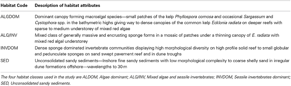
Table 2. Summary of the four category classification scheme used in the study.

Habitat classification

The Random Forests (RF) classification algorithm (Breiman, 2001) was used to quantify relationships between environmental data layers and video observations. The RF algorithm uses bootstrap samples of the training data and randomly selected subsets of available predictor variables to grow multiple classification trees. At each bootstrap iteration of the RF process the resultant tree is used to predict those data not included in the training process (“out of bag” or OOB observations) and calculate a misclassification rate. Probabilities of membership for the various classes are estimated by the proportions of OOB predictions in each class (Cutler et al., 2007). Each tree provides a unit vote for the most popular class at each input instance and the final classification label is determined by a majority vote of all trees in the ensemble.

Trees are left unpruned (i.e., fully fitted to the training data) in order to diminish potential bias introduced by any stopping rules. The algorithm yields an ensemble that can achieve both low bias and low variance (from averaging over a large ensemble of low-bias, high-variance but low correlation trees).

In this study the RF procedure was applied using a MATLAB implementation (Jaiantilal, 2009) of the code proposed by Breiman and Cutler (available online at http://www.stat.berkeley.edu/users/breiman/). The number of decision trees (ntree) was specified at 500 and variables selected from the pool of predictor variables for splitting at each node (m) was the square root of the number of available predictors, a value which has been commonly used in other implementations of the routine (Breiman, 2001; Cutler et al., 2007). Classification rules and importance measures were obtained from two separate implementations of the RF procedure. The first model included 12 predictor variables derived from and including the primary bathymetry and backscatter products (hereafter referred to as the MBES model). The procedure was run again with the addition of a grid layer representing annual maximum orbital velocity at the seabed (hereafter referred to as the wave energy model). The performance of the RF models was evaluated by comparing each one against a subset (30%) of video observation data that were withheld from the modeling process. Global accuracy of each model was established using confusion matrices (Overall accuracy and κ-statistic), similarly class specific accuracy was derived using metrics of user's and producer's accuracies.

Importance indices from each implementation of RF were obtained by randomly permuting the values for each input variable in the classification in the OOB samples for each tree. Decrease in accuracy caused by effectively removing a particular feature from a tree denotes its relevance to the classification accuracy of that tree. Changes in accuracy as a result of permutation were averaged across all trees in the forest and used to calculate a relative measure of variable importance (permutation importance measure) based on mean decrease in accuracy for each feature used in the classification across all classes.

Results

A model representing maximum bottom orbital velocity (u_max) was created using inputs from a global wave model attenuated by a bathymetric surface composed of coarse-scale (~270 m) regional bathymetry and then fine-scale (5 m) local bathymetry. Values of u_max ranged from 0.5 to 1.36 m/s (Figure 5). The spatial pattern of bottom orbital velocities reflects the bathymetry and orientation to surface wave conditions which arrive predominantly from the south-west quadrant. As a result, highly energetic hydrodynamic conditions at the seabed are evident in the western half of the site reducing to moderate conditions in the eastern portion of the site which is largely sheltered from prevailing wave conditions by Cape Otway.

FIGURE 5

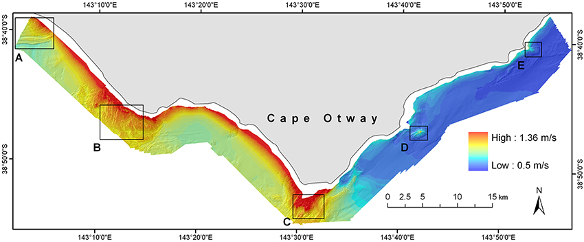
Figure 5. Distribution of modeled maximum orbital velocity (u_max) values across the Cape Otway study site for the year 2000. Maximum bottom orbital velocities were calculated by extending outputs of the local scale numerical wave model to the seabed using linear wave theory. Boxes (A–E) delineate major reef systems at the site and are analogous to those shown in Figure 1.

Cross-validated classification accuracy metrics corresponded well with those obtained from internal validation using the OOB data. The overall accuracy of the model that considered both MBES derived information and wave exposure was found to be higher (93%) than the model considering only the MBES derived predictors (88%). Accuracy as defined by κ was higher for the exposure classification (0.87) than the MBES classification (0.77). A pairwise test for significance of the κ statistic for each error matrix (Congalton and Green, 2009) revealed a significant difference between the two error matrices (z = 13.3) with the exposure model performing significantly better than the MBES model. User's and producer's accuracies for each habitat class were universally higher for the exposure model. Increase in accuracy was most evident for the ALG/INV class which was commonly misclassified as either ALGDOM or INVDOM in the MBES classification. Producer's accuracy increased from 47 to 76% and user's accuracy increased from 68 to 82% in this class with the addition of the exposure layer to the classification.

Further accuracy assessment was done to assess the relative influence of each set of predictor variables between the sheltered eastern side of the site and the more exposed west. Similar patterns of improved accuracy with the addition of the wave energy variable were observed in all cases. Accuracy gains in the east of the site, however, were comparatively small and non-significant (z = 1.82) (Table 3). The greatest increases in overall accuracy and corresponding κ-values were observed in the west of the site. Overall accuracy increased from 84 to 93%, and κ was significantly higher (z = 13.84), increasing from 0.75 to 0.89. Improvements in model accuracy corresponded largely with better discrimination of the ALGDOM and ALG/INV classes in the wave energy model. Producer's accuracy increased from 78% to 93% and 42% to 69% for each class respectively.

TABLE 3

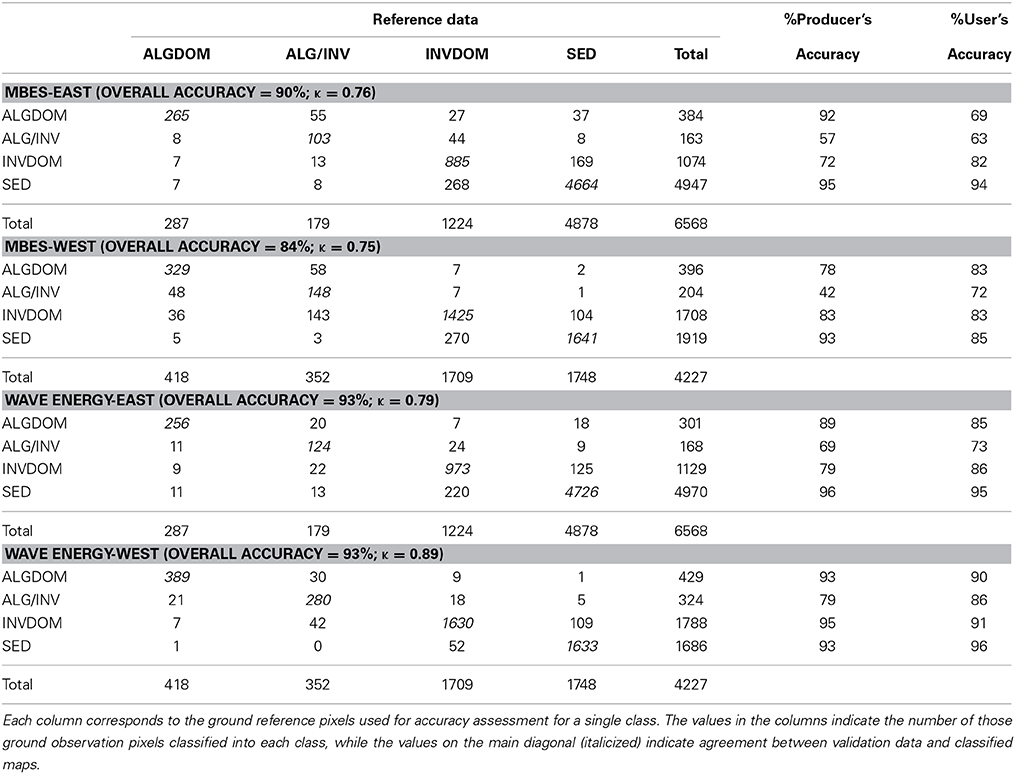
Table 3. Confusion matrices for the classified images derived from the MBES and wave energy models models east and west of Cape Otway.

Variables identified as most important over all classes for the MBES classification in order of decreasing importance were bathymetry, rugosity, the backscatter derivative HSIr and backscatter intensity (Figure 6). These predictors were also most important in varying degrees to the discrimination of individual habitat classes except for the ALG/INV class which was not well resolved by backscatter intensity. Maximum curvature, the variables representing aspect (northness and eastness) and Benthic Position Index (BPI) were the least important predictors across all habitat classes.

FIGURE 6

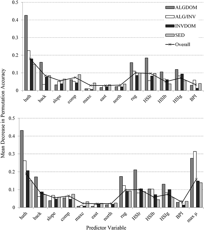
Figure 6. Variable importance assessed by mean decrease in permutation accuracy obtained from the Random Forests classification (y-axis). Mean decrease in permutation accuracy is calculated using the difference between the misclassification rate of the out of bag (OOB) data, and the misclassification rate if values of a given variable are randomly permuted for the OOB observations and passed down the tree to create new predictions. Results from the model incorporating only MBES predictor variables are shown in the top graph, while those incorporating both MBES predictors and modeled maximum bottom orbital velocity are shown at bottom. Variable codes on the x-axis are detailed in Table 2.

The introduction of the wave energy variable to the classification did not appreciably change the relative patterns of contribution of the MBES variables to classification accuracy. The wave energy proxy u_max was identified as an important feature (second only to bathymetry) across all habitat classes except for the ALG/INV class where it was of primary importance to the discrimination of that class from all others. The relationship between depth, wave energy and habitat categories east and west of Cape Otway is evident in Figure 7. Habitat classes are particularly well partitioned along the wave energy axis into observations made west and east of Cape Otway. Observations occurring west of Cape Otway display higher separability between classes, again along the wave energy axis, than those east of Cape Otway which overlap along the depth axis.

FIGURE 7

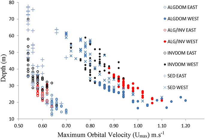
Figure 7. Depth (y-axis) plotted against maximum bottom orbital velocity (u_max) for classified video observations. Hollow circles indicate observations from east of the study site and filled circles those from the west. Habitat classes are described in Table 2. ALGDOM, Algal dominated reef; ALG/INV, mixed algae and sessile invertebrates; INVDOM, reef with sessile invertebrates; SED, unconsolidated sandy sediments.

Decision rules derived from the two RF classifications were executed over the full extents of their respective sets of predictor variables to create full coverage habitat maps of the site. Class coverages in the MBES classification were lower for the ALGDOM class (8.7%) and the SED class (3.5%) (Table 4) and higher for the INVDOM class (8.8%). Most notably, the area covered by the ALG/INV class was 33.8% greater in the wave energy classification than the MBES classification.

TABLE 4

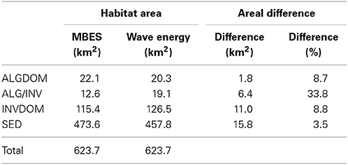
Table 4. Class area estimations and areal differences derived from the model containing only MBES variables (Acoustic) and the model containing both MBES and wave energy variables.

Major contiguous reef systems at the site, (identified in Figures 1, 4), from the exposed western end of the site (Reef A) through to its more sheltered eastern extent (Reef E) showed a clear trend in the zonation of benthic habitat types achieved by each of the models in the study. In the exposed west of the site the MBES classification predicted a zone of change (ALG/INV) between the ALGDOM and INVDOM classes in accordance with other areas of reef at similar depths, although there are no records of that habitat in the ground observations (Figure 8). The wave energy classification however, showed an obvious delineation between macroalgal dominated reef and invertebrate dominated reef with the ALGDOM class extending to ~34 m, notably deeper than at any other area of the site.

FIGURE 8

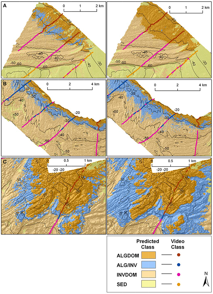
Figure 8. Classified habitat maps of representative reef systems west of Cape Otway overlaid with classified observation data from towed video transects. Locations of reefs A, B and C are shown in Figures 1, 4. Classifications on the left hand side of the figure were derived using MBES only variables, while those on the right were derived using both MBES predictor variables and maximum bottom orbital velocities.

Reef systems depicted in insets B and C showed an opposing trend. While reef coverage of the ALGDOM class appear very similar, predictions of the ALG/INV class by the wave energy model showed it to cover a considerably more extensive area and extend to greater depths (ca.40 m) than the MBES model (ca.32 m). It also appears that these areas of the site may be the principal source of differences in estimated area of the ALG/INV class between the two classifications.

By contrast, there appear to be only relatively small differences between the two habitat classifications on the sheltered eastern side of the site (Reefs D and E). Both classifications visually show a similar pattern of habitat distributions.

Discussion

This study has demonstrated that a reef habitat classification model incorporating modeled wave-induced orbital velocity performs significantly better than one incorporating indirect proxies derived from depth and seafloor morphology in describing patterns of benthic habitat distribution at a wave-exposed site in temperate Australia. Improvement in the model was largely due to increased classification capacity of shallow reef habitat types along a gradient of wave energy, allowing their distribution to be more accurately predicted. This pattern corroborated with cross-validation measures which showed an improvement in the classification accuracy for all habitat categories defined in the study. The area covered by each habitat class differed between the two models. Differences were most evident in a transitional habitat between algal dominated reefs and reefs characterized by sponge dominated sessile invertebrates.

In the present investigation, variables of primary importance to classification accuracy of the best performing model were bathymetry, bottom orbital velocity, rugosity, backscatter intensity and HSI backscatter derivatives. A similar pattern is reported by Bekkby et al. (2009) in their distribution modeling study of the kelp Laminaria hyperborea where depth, terrain curvature, wave and light exposure were found to be the most important geophysical factors explaining the distribution of the species. Similarly depth, slope, wave and light exposure were found to best explain the potential distribution of the fucoid kelp Saccharina latissima in Norwegian waters (Bekkby and Moy, 2011).

Differentiation of benthic habitats in this study was also largely determined by proxies of light availability (bathymetry), availability of suitable substrate for attachment (rugosity) and hydrodynamic energy (seabed orbital velocity). While the contribution of backscatter intensity and its HSI derivatives is more difficult to interpret. It is surmised that these products are important to the classifier in distinguishing textural differences between inhomogeneous substrate types that are indicative of suitable areas for attachment of sessile species.

The high relative contribution of the depth and wave energy variables in explaining habitat distribution, in particular for the two classes defined by the presence of the canopy forming kelp E. radiata (ALG/INV and ALGDOM), is well supported by the ecological relevance of these features in explaining distribution of the species. Bathymetry acts as an indirect mediator for light availability, and limits the depth at which the basic requirements for photosynthesis can be met. The influence of wave energy is also attenuated by depth although it is evident that bathymetry alone did not capture the full influence of wave energy as a variable structuring the distribution of habitats across the site. Differences between classifications can be attributed largely to the contrasting regimes of wave energy on each side of Cape Otway. When analyzed independently, classification accuracy for the eastern section of the site did not improve significantly with the addition of the bottom orbital velocity variable which was limited in its range from 0.54 to 0.74 ms⁻¹. This indicates that the variable describing bottom orbital velocity improves the predictive capacity of the model only where wave energy is a more restrictive environmental factor. In both models the kelp dominated (ALGDOM) class transitions to invertebrate dominated reef (INVDOM) through a narrow depth band (5–7 m) of the mixed algae and invertebrates class (ALG/INV) (Figure 9, reefs D and E). The kelp E. radiata is restricted in vertical distribution to depths less than 30 m beyond which invertebrate dominated reef becomes the primary reef habitat type.

FIGURE 9

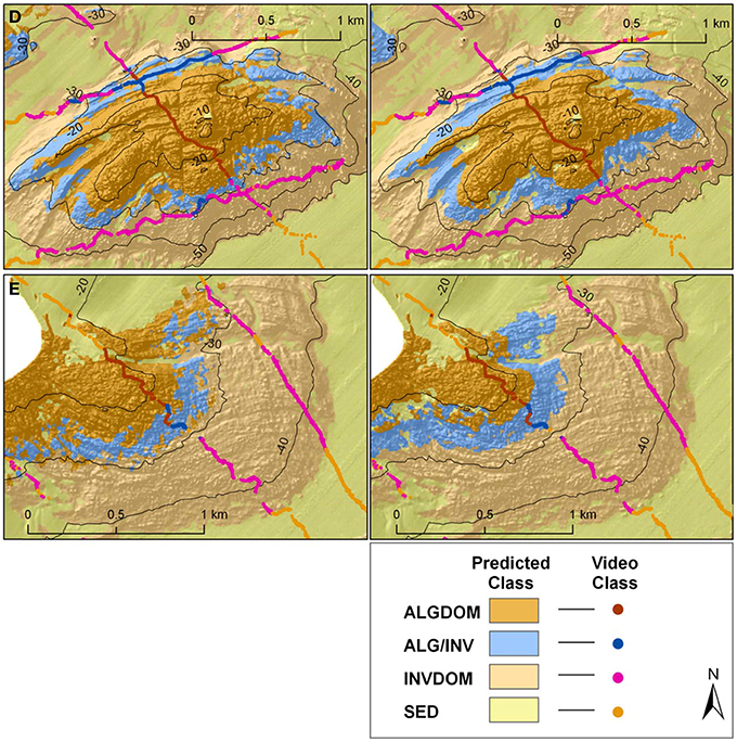
Figure 9. Classified habitat maps of representative reef systems east of Cape Otway overlaid with classified observation data from towed video transects. Locations of reefs D and E are shown in Figures 1, 4. Classifications on the left hand side of the figure were derived using MBES variables alone, while those on the right were derived using MBES variables and maximum bottom orbital velocities.

West of Cape Otway a different pattern emerges, with observations of E. radiata extending to depths of 49 m and the transition zone between algal and invertebrate dominated reef types spanning a greater depth range (~25 m). This east-west variation in depth distributions is captured to some extent by the model incorporating only MBES variables which predicts the ALG/INV class occurring marginally deeper (33 m) than in the east but is better described by the wave energy model which predicts the ALG/INV class to occur both deeper (42 m) and across a greater depth range (~20 m).

Differences in patterns of distribution of the ALGDOM class between reef A, and reefs B and C on the western side of the site are potentially caused by a temporal mismatch in collection of observation data which in MBES survey block 1 (Figure 1) was collected 2 years prior to the remainder of the study site. Although observation data were collected in February of each year there is evidence to suggest that canopy density of E. radiata is temporally variable and largely dependent on the timing of optimum environmental conditions conducive to growth, for example, temperature, nutrient and light availability (Wernberg and Goldberg, 2008). It is therefore conceivable that the observation data associated with survey block 1 represents a different stage on the annual senescence to peak biomass cycle of the species and in that respect is not consistent with observational data from the rest of the site.

Alternatively, these differences may reflect the interaction of incoming wave energy with local reef geometry which is noticeably different between reefs. Reef A displays a relatively steep and regular offshore gradient with little topographic diversity descending to depths of 60 m close to the coast. Reefs depicted in insets B and C by comparison have a shallower offshore gradient and are characterized by rugged terrain composed of medium to high-profile crests (<1–2 m), troughs and ridges extending farther offshore. While modeled maximum orbital velocity is of similar magnitude for all of these areas, the complexity of the reef surface at areas B and C may provide a wider range of hydrodynamic conditions caused by localized topographic diversity allowing the establishment of invertebrate communities in a mosaic of lower flow areas within the reef. This theory is corroborated by the work of Toohey and Kendrick (2008) who linked greater species richness on reefs with complex topography to a reduction in the structuring effects of E. radiata canopy on understorey communities.

Our results suggest that the importance of depth as a predictor of reef habitat distribution is strongly mediated by variation in hydrodynamic energy. This may indicate that light is not the limiting factor in the vertical distribution of E. radiata in the east of the site. The limited depths attained by the species compared to the west of the site are potentially the result of competitive interactions with sessile invertebrates for limited hard substrata suitable for attachment. Under this assumption it can also be suggested that stronger wave energy conditions in the west of the site afford some measure of competitive advantage to E. radiata allowing the species to successfully occupy space to a greater depth. This contention is supported by the known ecology of the species which exhibits a plastic morphology in response to hydrodynamic stress. Individuals at exposed sites have been reported to display drag reducing morphological characters such as smaller size, narrower laterals and blades as well as thicker holdfasts and stipes (Wernberg and Thomsen, 2005; Wernberg and Vanderklift, 2010). Higher energy conditions may additionally mediate the influence of E. radiata on understorey communities through increased effects of direct physical abrasion by fronds (Toohey et al., 2004; Fowler-Walker et al., 2005). There is also evidence to suggest that some kelp species achieve a higher rate of primary productivity, increasing both individual density and canopy biomass in high vs. low wave energy environments (Hurd, 2000). Pedersen et al. (2012) relate this pattern to higher epiphytic load and self-shading in low energy sites and speculate that higher energy conditions may increase light availability to the canopy through continuous and frequent movement.

The results presented have increased our knowledge of the structuring effects of wave energy on subtidal habitats and demonstrated its relevance to benthic habitat mapping. There are however a number of limitations concerning derivation of the wave energy model that should be considered when interpreting these results. Foremost, the temporal resolution of the spectral wave model used to calculate orbital velocity at the seabed is restricted to a single year which may not have fully captured the upper range of extreme wave conditions experienced at the site. Significant wave heights modeled in this study did not exceed 6.2 m for the year 2000 although Hemer et al. (2008) estimate a centennial return significant wave height of 15.51 m for Cape Sorell and cite a 13.2 m event measured by the wave buoy in 1985. Therefore, habitat structuring by wave energy at the site could well be the result of larger wave events occurring outside the temporal resolution of the study.

Secondly, the spatial grain of the wave energy model (60 m) was observed in a small number of cases to cause block artifacts in the habitat classification, predominantly in the areas classified as ALG/INV. This is presumably a function of the value of the wave energy dataset in defining these areas and is of consequence as it potentially masks fine-scale variation in habitat boundaries important in analysis of patch metrics (e.g., Ierodiaconou et al., 2011).

Exposure to hydrodynamic energy is one of the fundamental variables of the coastal environment (Nishihara and Terada, 2010) and has been well demonstrated to play in integral role in the life histories and evolutionary biology of the organisms found there (Hurd, 2000). There is a wealth of evidence to suggest that the degree of adaptation to varying levels of hydrodynamic energy strongly influences the available niche of many species. Despite the evidence linking the distributional ecology of marine taxa to the physical aspects of their hydrodynamic environment, there are relatively few studies (e.g., Galparsoro et al., 2013) that explore the application of these variables for local-scale (10's–100's km²) predictive distribution modeling. In this study benthic habitats at a wave-exposed site were characterized according to environmental variables obtained from MBES variables only, and compared with a characterization based on the addition of a fine-scale wave energy model. Measures of classification accuracy obtained with the addition of the wave energy variable to the model were significantly higher overall and contributed to greater resolvability between habitat classes than MBES derived variables alone. Furthermore, an insight was gained into the interaction between the structuring effects of depth (a proxy for light availability) and exposure to wave energy over the full depth range of a foundation kelp species that affects biodiversity and ecological functioning on shallow reefs across temperate Australasia. This study highlights the suitability of exposure measures for predictive benthic habitat modeling on wave-exposed coastlines and provides a basis for continuing research relating patterns of biological distribution to measurable aspects of the physical environment.

Conflict of Interest Statement

The authors declare that the research was conducted in the absence of any commercial or financial relationships that could be construed as a potential conflict of interest.

Acknowledgments

DI conceived the project and led the fieldwork. AR led the analyses and writing with contributions from DI and TW. This work was supported by the National Heritage Trust and Caring for Country as part of the Victorian Marine Habitat Mapping Project with project partners Glenelg Hopkins Catchment Management Authority, Department of Environment and Primary Industries, Parks Victoria, University of Western Australia and Fugro Survey. We thank the crew from the Australian Maritime College research vessel Bluefin, which was used for the multibeam data collection. We also thank the crew from Deakin University research vessel Courageous II for assisting DI and AR collecting the towed video data used in this project. Thanks to Richard Zavalas for assistance with the validation matrices. GIS laboratory facilities at Deakin University, Warrnambool, Victoria were used for spatial analyses. We also thank the three reviewers for their constructive suggestions to improve the manuscript.

Footnotes

1. ^Available online at: http://www.dhigroup.com/ [Accessed 20/08 2012].

References

Airoldi, L. (2003). The effects of sedimentation on rocky coast assemblages. Oceanogr. Mar. Biol. 41, 161–236. doi: 10.1016/S0022-0981(96)02770-0

CrossRef Full Text | Google Scholar

Bekkby, T., Isachsen, P. E., Isaeus, M., and Bakkestuen, V. (2008). GIS modeling of wave exposure at the seabed: a depth-attenuated wave exposure model. Mar. Geod. 31, 117–127. doi: 10.1080/01490410802053674

CrossRef Full Text | Google Scholar

Bekkby, T., and Moy, F. E. (2011). Developing spatial models of sugar kelp (Saccharina latissima) potential distribution under natural conditions and areas of its disappearance in Skagerrak. Estuarine Coast. Shelf Sci. 95, 477–483. doi: 10.1016/j.ecss.2011.10.029

CrossRef Full Text | Google Scholar

Bekkby, T., Rinde, E., Erikstad, L., and Bakkestuen, V. (2009). Spatial predictive distribution modelling of the kelp species Laminaria hyperborea. Ices J. Mar. Sci. 66, 2106–2115. doi: 10.1093/icesjms/fsp195

CrossRef Full Text | Google Scholar

Bell, J. J., and Barnes, D. K. A. (2000). The distribution and prevalence of sponges in relation to environmental gradients within a temperate sea lough: vertical cliff surfaces. Divers. Distrib. 6, 283–303. doi: 10.1046/j.1472-4642.2000.00091.x

CrossRef Full Text | Google Scholar

Boulding, E. G., Holst, M., and Pilon, V. (1999). Changes in selection on gastropod shell size and thickness with wave-exposure on Northeastern Pacific shores. J. Exp. Mar. Biol. Ecol. 232, 217–239. doi: 10.1016/S0022-0981(98)00117-8

CrossRef Full Text | Google Scholar

Breiman, L. (2001). Random forests. Mach. Learn. 45, 5–32. doi: 10.1023/A:1010933404324

CrossRef Full Text | Google Scholar

Chollett, I., and Mumby, P. J. (2012). Predicting the distribution of Montastraea reefs using wave exposure. Coral Reefs 31, 493–503. doi: 10.1007/s00338-011-0867-7

CrossRef Full Text | Google Scholar

Congalton, R. G., and Green, K. (2009). Assessing the Accuracy of Remotely Sensed Data: Principles and Practices. Boca Raton, FL: CRC Press.

Google Scholar

Cutler, D. R., Edwards, T. C., Beard, K. H., Cutler, A., and Hess, K. T. (2007). Random forests for classification in ecology. Ecology 88, 2783–2792. doi: 10.1890/07-0539.1

Pubmed Abstract | Pubmed Full Text | CrossRef Full Text | Google Scholar

Denny, M. (2006). Ocean waves, nearshore ecology, and natural selection. Aquat. Ecol. 40, 439–461. doi: 10.1007/s10452-004-5409-8

CrossRef Full Text | Google Scholar

Ekebom, J., Laihonen, P., and Suominen, T. (2003). A GIS-based step-wise procedure for assessing physical exposure in fragmented archipelagos. Estuarine Coast. Shelf Sci. 57, 887–898. doi: 10.1016/S0272-7714(02)00419-5

CrossRef Full Text | Google Scholar

England, P. R., Phillips, J., Waring, J. R., Symonds, G., and Babcock, R. (2008). Modelling wave-induced disturbance in highly biodiverse marine macroalgal communities: support for the intermediate disturbance hypothesis. Mar. Freshw. Res. 59, 515–520. doi: 10.1071/MF07224

CrossRef Full Text | Google Scholar

Fonseca, M. S., and Bell, S. S. (1998). Influence of physical setting on seagrass landscapes near Beaufort, North Carolina, USA. Mar. Ecol. Prog. Ser. 171, 109–121. doi: 10.3354/meps171109

CrossRef Full Text | Google Scholar

Foster, S. D., Bravington, M. V., Williams, A., Althaus, F., Laslett, G. M., and Kloser, R. J. (2009). Analysis and prediction of faunal distributions from video and multi-beam sonar data using Markov models. Environmetrics 20, 541–560. doi: 10.1002/env.952

CrossRef Full Text | Google Scholar

Fowler-Walker, M. J., Gillanders, B. M., Connell, S. D., and Irving, A. D. (2005). Patterns of association between canopy-morphology and understorey assemblages across temperate Australia. Estuarine Coast. Shelf Sci. 63, 133–141. doi: 10.1016/j.ecss.2004.10.016

CrossRef Full Text | Google Scholar

Friedlander, A. M., Brown, E. K., Jokiel, P. L., Smith, W. R., and Rodgers, K. S. (2003). Effects of habitat, wave exposure, and marine protected area status on coral reef fish assemblages in the Hawaiian archipelago. Coral Reefs 22, 291–305. doi: 10.1007/s00338-003-0317-2

CrossRef Full Text | Google Scholar

Galparsoro, I., Borja, Á., Kostylev, V. E., Rodríguez, J. G., Pascual, M., and Muxika, I. (2013). A process-driven sedimentary habitat modelling approach, explaining seafloor integrity and biodiversity assessment within the European Marine Strategy Framework Directive. Estuar. Coast. Shelf Sci. 131, 194–205. doi: 10.1016/j.ecss.2013.07.007

CrossRef Full Text | Google Scholar

Greenlaw, M. E., Roff, J. C., Redden, A. M., and Allard, K. A. (2011). Coastal zone planning: a geophysical classification of inlets to define ecological representation. Aquat. Conserv. Mar. Freshw. Ecosyst. 21, 448–461. doi: 10.1002/aqc.1200

CrossRef Full Text | Google Scholar

Harris, P. T., and Hughes, M. G. (2012). Predicted benthic disturbance regimes on the Australian continental shelf: a modelling approach. Mar. Ecol. Prog. Ser. 449, 13–25. doi: 10.3354/meps09463

CrossRef Full Text

Hemer, M. A., Simmonds, I., and Keay, K. (2008). A classification of wave generation characteristics during large wave events on the Southern Australian margin. Cont. Shelf Res. 28, 634–652. doi: 10.1016/j.csr.2007.12.004

CrossRef Full Text | Google Scholar

Hill, N. A., Pepper, A. R., Puotinen, M. L., Hughes, M. G., Edgar, G. J., Barrett, N. S., et al. (2010). Quantifying wave exposure in shallow temperate reef systems: applicability of fetch models for predicting algal biodiversity. Mar. Ecol. Prog. Ser. 417, 83–95. doi: 10.3354/meps08815

CrossRef Full Text | Google Scholar

Hughes, M. G., and Heap, A. D. (2010). National-scale wave energy resource assessment for Australia. Renewable Energy 35, 1783–1791. doi: 10.1016/j.renene.2009.11.001

CrossRef Full Text | Google Scholar

Hurd, C. L. (2000). Water motion, marine macroalgal physiology, and production. J. Phycol. 36, 453–472. doi: 10.1046/j.1529-8817.2000.99139.x

CrossRef Full Text | Google Scholar

Ierodiaconou, D., Monk, J., Rattray, A., Laurenson, L., and Versace, V. L. (2011). Comparison of automated classification techniques for predicting benthic biological communities using hydroacoustics and video observations. Cont. Shelf Res. 31, S28–S38. doi: 10.1016/j.csr.2010.01.012

CrossRef Full Text | Google Scholar

Jaiantilal, A. (2009). Classification and Regression by Random Forest—MATLAB [Online]. Available online at: http://code.google.com/p/randomforest-matlab/ [Accessed November 10th 2013].

Kostylev, V. E., and Hannah, C. G. (2007). “Process-driven characterization and mapping of seabed habitats,” in Mapping the Seafloor for Habitat Characterization, eds B. J. Todd and H. G. Greene (St John's, NL: Geological Society of Canada), 171–184.

Letourneur, Y. (1996). Dynamics of fish communities on Reunion fringing reefs, Indian Ocean.1. Patterns of spatial distribution. J. Exp. Mar. Biol. Ecol. 195, 1–30. doi: 10.1016/0022-0981(95)00089-5

CrossRef Full Text | Google Scholar

Lindegarth, M., and Gamfeldt, L. (2005). Comparing categorical and continuous ecological analyses: effects of “wave exposure” on rocky shores. Ecology 86, 1346–1357. doi: 10.1890/04-1168

CrossRef Full Text | Google Scholar

Nishihara, G. N., and Terada, R. (2010). Species richness of marine macrophytes is correlated to a wave exposure gradient. Phycological Res. 58, 280–292. doi: 10.1111/j.1440-1835.2010.00587.x

CrossRef Full Text | Google Scholar

Pedersen, M. F., Nejrup, L. B., Fredriksen, S., Christie, H., and Norderhaug, K. M. (2012). Effects of wave exposure on population structure, demography, biomass and productivity of the kelp Laminaria hyperborea. Mar. Ecol. Prog. Ser. 451, 45–60. doi: 10.3354/meps09594

CrossRef Full Text | Google Scholar

Pfaff, M. C., Branch, G. M., Wieters, E. A., Branch, R. A., and Broitman, B. R. (2011). Upwelling intensity and wave exposure determine recruitment of intertidal mussels and barnacles in the southern Benguela upwelling region. Mar. Ecol. Prog. Ser. 425, 141–152. doi: 10.3354/meps09003

CrossRef Full Text | Google Scholar

Porter-Smith, R., Harris, P. T., Andersen, O. B., Coleman, R., Greenslade, D., and Jenkins, C. J. (2004). Classification of the Australian continental shelf based on predicted sediment threshold exceedance from tidal currents and swell waves. Mar. Geol. 211, 1–20. doi: 10.1016/j.margeo.2004.05.031

CrossRef Full Text | Google Scholar

Rattray, A., Ierodiaconou, D., Laurenson, L., Burq, S., and Reston, M. (2009). Hydro-acoustic remote sensing of benthic biological communities on the shallow South East Australian continental shelf. Estuar. Coast. Shelf Sci. 84, 237–245. doi: 10.1016/j.ecss.2009.06.023

CrossRef Full Text | Google Scholar

Rattray, A., Ierodiaconou, D., Monk, J., Versace, V. L., and Laurenson, L. J. B. (2013). Detecting patterns of change in benthic habitats by acoustic remote sensing. Mar. Ecol. Prog. Ser. 477, 1–13. doi: 10.3354/meps10264

CrossRef Full Text | Google Scholar

Thomsen, M. S., Wernberg, T., and Kendrick, G. A. (2004). The effect of thallus size, life stage, aggregation, wave exposure and substratum conditions on the forces required to break or dislodge the small kelp Ecklonia radiata. Botanica Marina 47, 454–460. doi: 10.1515/BOT.2004.068

CrossRef Full Text | Google Scholar

Thomson, D. P., Babcock, R. C., Vanderklift, M. A., Symonds, G., and Gunson, J. R. (2012). Evidence for persistent patch structure on temperate reefs and multiple hypotheses for their creation and maintenance. Estuar. Coast. Shelf Sci. 96, 105–113. doi: 10.1016/j.ecss.2011.10.014

CrossRef Full Text | Google Scholar

Toohey, B. D., and Kendrick, G. A. (2008). Canopy-understorey relationships are mediated by reef topography in Ecklonia radiata kelp beds. Eur. J. Phycol. 43, 133–142. doi: 10.1080/09670260701770554

CrossRef Full Text | Google Scholar

Toohey, B., Kendrick, G. A., Wernberg, T., Phillips, J. C., Malkin, S., and Prince, J. (2004). The effects of light and thallus scour from Ecklonia radiata canopy on an associated foliose algal assemblage: the importance of photoacclimation. Mar. Biol. 144, 1019–1027. doi: 10.1007/s00227-003-1267-5

CrossRef Full Text | Google Scholar

Turner, S. J., Hewitt, J. E., Wilkinson, M. R., Morrisey, D. J., Thrush, S. F., Cummings, V. J., et al. (1999). Seagrass patches and landscapes: the influence of wind-wave dynamics and hierarchical arrangements of spatial structure on macrofaunal seagrass communities. Estuaries 22, 1016–1032. doi: 10.2307/1353080

CrossRef Full Text | Google Scholar

Wernberg, T., and Goldberg, N. (2008). Short-term temporal dynamics of algal species in a subtidal kelp bed in relation to changes in environmental conditions and canopy biomass. Estuar. Coast. Shelf Sci. 76, 265–272. doi: 10.1016/j.ecss.2007.07.008

CrossRef Full Text | Google Scholar

Wernberg, T., and Thomsen, M. S. (2005). The effect of wave exposure on the morphology of Ecklonia radiata. Aquat. Bot. 83, 61–70. doi: 10.1016/j.aquabot.2005.05.007

CrossRef Full Text | Google Scholar

Wernberg, T., and Vanderklift, M. A. (2010). Contribution of temporal and spatial components to morphological variation in the kelp Ecklonia (Laminariales). J. Phycol. 46, 153–161. doi: 10.1111/j.1529-8817.2009.00772.x

CrossRef Full Text | Google Scholar

Whiteway, T. (2009). Australian Bathymetry and Topography Grid, June 2009. Scale 1:5000000. Canberra, ACT: Geoscience Australia.

Zavalas, R., Ierodiaconou, D., Ryan, D., Rattray, A., and Monk, J. (2014). Habitat classification of temperate marine macroalgal communities using bathymetric LiDAR. Remote Sens. 6, 2154–2175. doi: 10.3390/rs6032154

CrossRef Full Text | Google Scholar