Uncertainty, Irreversibility and the Optimal Timing of Large-Scale Investments in Protected Species Habitat Restoration

Introduction

Investments in ecosystem restoration projects are often subject to economic analyses to help determine which investments to make. Decisions on restoring critical habitat for protected species are complicated by the facts that costs are largely irretrievable and that delay in undertaking restoration can lead to further irreversible ecosystem damage (e.g., species extinction). When considering large-scale habitat restoration or species recovery projects, decision-makers typically face a variety of uncertainties such as current and future ecosystem conditions, the costs and efficacy of restoration efforts, and the presence of tipping points that must be weighed in the decision making process. Uncertainty regarding restoration efficacy, creating sunk restoration costs, and waiting for new information are valid reasons for delaying restoration. Conversely, the possibility ongoing ecosystem degradation that leads to higher restoration costs or irreversible system damage may lead decision-makers to move forward on restoration projects. These countervailing incentives are pervasive in restoration planning; hence there is a need for decision makers to be able to understand both reasons to hasten restoration efforts and reasons to slow them down within a single framework.

In this article we construct a model that highlights how uncertainty and the irreversible nature of many protected resource recovery investments create countervailing incentives that complicate decisions regarding whether and when to undertake an expensive project. Importantly, our model captures the tensions in such a decision: delaying action postpones costly expenditures and allows one to wait for more information, but delay also carries the risk of serious consequences such as species extinction. We formulate a continuous-time, continuous-state optimal stopping model of the decision of when to remove a dam and restore the ecosystem. We solve the model using stochastic dynamic programming methods. These types of models are prevalent in the “real options” literature (see Dixit and Pindyck, 1994) and in the investment management literature for pricing options.

One good example of a large investment in ecosystem restoration when uncertainty is present is the decision regarding when (and whether) to remove a large dam to improve habitat conditions for anadromous fish. This problem exists, for example, when undertaking recovery action for protected Evolutionarily Significant Units of Pacific salmon species on the west coast of North America. Dams create a number of problems for aquatic ecosystems (Ligon et al., 1995; Bednarek, 2001; Bunn and Arthington, 2002; Pringle, 2003; Beechie et al., 2006; Pess et al., 2008). Dams block access to upstream habitat thus often greatly reducing the carrying capacity for anadromous fish. Dams also disrupt natural hydrologic regimes, which can lead to degradation of water quality, lack of nutrients, and adverse changes in stream geomorphology. We use the example of an expensive dam removal project to motivate our model, but other similar examples are possible, such as the purchase of a large plot of land that is uniquely important habitat for protected species or constructing a new wastewater treatment plant to improve water quality (Connon et al., 2011; Parker et al., 2012; Medellín-Azuara et al., 2013).

A key feature of ecosystem recovery decisions is that there are risks involved. For example, fish population viability is affected by human-induced stressors that can be alleviated through mitigation or restoration measures. In our case, a dam may block access to spawning habitat and alter hydrologic regimes. Fish populations, however, are also subject to random fluctuations caused by stochastic environmental factors. Therefore, we do not know with certainty ex ante whether fish populations will maintain their current levels, increase, or decline even after the dam is removed. The path that future ecosystem costs will take is uncertain. At any time, there is a risk that populations of concern could drop below a threshold leading to extinction. In fact, results from the ecology literature indicate that small populations are at greater risk of crossing these thresholds because their small size increases the relative variability in the population (Lande, 1993; McElhany et al., 2000). In a decision model context, reaching a point of extinction can be thought of as an extreme high-cost state.

Real options analysis is an attractive framework for analyzing large-scale ecosystem restoration projects because it captures three important features. First, restoration is costly and can be irreversible. For example, the cost of a restoration project on the Elwha River in Washington, including removal of two large dams, was estimated to be $324.7 million (National Park Service, 2005). Second, there is significant uncertainty regarding future ecosystem costs if major restoration is not undertaken. For example, the evolution of fish populations is uncertain and affected by restoration or the lack thereof. Declining fish populations and possible extinction create societal costs. Third, damage to ecosystems, such as species extinction, can become irreversible if restoration is delayed for too long. For example, one recent article extrapolates current trends in fish population dynamics and concludes that 9 out of 21 anadromous salmonid taxa in California are “in danger of extinction in the near future” (Katz et al., 2013). The authors note that large-scale habitat restoration projects such as dam removal will become increasingly important in the face of warming temperatures and more variable rainfall.

Economic analysis that evaluates expenditures on protected resources conservation can help decide whether, where, and how much to invest. Previous studies constructed models to solve for cost-effective allocation of limited resources for habitat restoration (Duke et al., 2013). One example is work that chooses the optimal spatial allocation of riparian habitat restoration to help in the recovery of protected steelhead trout (Wu et al., 2000; Wu and Skelton-Groth, 2002). Benefit-cost analysis, which provides a test of whether projects are likely to improve social welfare, is often used and cited in decisions regarding whether or not to undertake ecosystem restoration projects (Pearce, 1998; Hanley, 2001; Hammitt, 2013). However, traditional benefit-cost analysis misses important aspects of the investment decision when planning for large, irreversible investments in cases where protected species are at risk of extinction. Verbruggen (2013) discusses the concept of irreversibility and its importance in decision-making. Verbruggen (2013) also highlights some limitations of traditional cost-benefit analysis. Our modeling efforts address some of these concerns by directly incorporating irreversibility (both in terms of sunk investment costs and irreparable harm to ecosystems), uncertainty (in terms of stochastically evolving biological resources), and timing issues.

The decision of when to restore an ecosystem is also similar to the question of when to invest in expensive pollution control. Pindyck (2000, 2002) considers a model of when to invest in pollution control, focusing on irreversibility and uncertainty. By investing immediately in pollution control, Pindyck notes that society pays sunk costs in pollution control investments (for example scrubbers on coal plants). These types of sunk costs (i.e., irreversible investments) lead one to favor delaying investment. Conversely, potential permanent environmental damages that may be very costly or impossible to reverse (e.g., permanent temperature changes from greenhouse gas emissions) lead one to hasten the decision. Pindyck characterizes these types of damages as sunk benefits. These two types of irreversibilities, sunk benefits and sunk costs, are countervailing—one hastens the decisions to act and the other delays the decision to act.

Some previous work uses a real options framework to examine natural resource management problems when uncertainty and irreversibility exist. Saphores and Shogren (2005) formulate a model of invasive species and pest control. In this model, damages from pests are irreversible and there is uncertainty in how fast the pest population will grow. Saphores and Shogren's (2005) model is interesting in our context because invasive species control is an ecosystem improvement investment. Conrad (2000) presents a model of when to develop (or extract resources from) a wilderness area. The social value of the wilderness area, the value of the extractable resource, and the benefit flow from development in the future are all uncertain while development is irreversible. The irreversibility of the development creates an option value that creates an incentive to preserve the wilderness area. Similarly, Leroux et al. (2009) develop a real options model of land conversion with stochastic future environmental damages. Saphores (2003) formulates a model to determine the harvest size of a renewable resource. Similar to our approach here, Saphores (2003) incorporates the risk of extinction in the decision model, showing that potential extinction creates an incentive to reduce harvest levels.

Our model includes a single ecosystem cost function that incorporates two different sources of uncertainty that are important to the results: uncertainty (variability) in the future time path of ecosystem costs that are generated by a large dam and uncertainty regarding whether the ecosystem will jump to an undesirable state (such as species extinction). Results from our model show that the sunk costs associated with a large investment combined with uncertainty regarding future ecosystem costs create an incentive to delay action that might help protected species recovery. The results also show a countervailing incentive to hasten the same investment when there is a risk that a species may become extinct. These results are predictable given the results of previous work (particularly Pindyck on pollution control cited above). Any irreversible cost in the presence of uncertain future benefits will create option value, while incorporating risk of moving to any extremely undesirable state creates an incentive to take action earlier. However, our work is novel in that it applies option pricing model to the issue of what action to take when attempting to recover threatened species. In contrast to the previous work on species extinction and conservation, the irreversibility in the model comes from the sunk cost associated with the expensive restoration action, rather than in the irreversible loss of ecosystem function. Our specification makes the problem applicable to species recovery efforts in a way not considered previously. In the Model section below, we construct a dynamic model that incorporates the uncertainties and irreversible outcomes just discussed. This is followed by a Results section that describes the outcomes of the model under different assumptions and demonstrates how different uncertainties and irreversible outcomes affect the decision. The final section is a discussion of these results and provides concluding comments.

Model

Here we formulate a model of whether to remove a dam before the end of its productive life. The objective is to maximize social welfare generated by a large dam. Social welfare is determined by the net benefits from the dam's operation—services such as hydropower, water supply and flood control less ecological costs such as negative benefits associated with reduced fish populations. In managing an ecological recovery decision like this, a decision-maker will monitor a variable or variables of interest to trigger a decision. In our model specification, the decision-maker monitors ecosystem costs (damages) imposed by the dam. We formulate an optimal stopping model where a decision-maker monitors the flow of net benefits from operating the dam over time and determines the conditions under which it is optimal to remove the dam prior to the end of its production life. In solving the dynamic problem we have specified, we assume the dam has T years of production life left. Upon reaching T years the dam must be removed, at cost K, if it has not been removed prior to reaching T years. The dam will be removed earlier than time T if the costs exceed the benefits by a threshold that is determined within the model. When the dam is removed we assume society absorbs a lump cost, equal to removal costs plus discounted residual ecological costs and foregone net benefits from operating the dam.

The benefits of dam removal in our model are due to reduced ecosystem costs. That is, we do not include a variable for ecosystem health level directly, but rather include dam-related ecosystem damages as a cost. This avoids having to map ecosystem health to a cost or to a utility received from poor ecosystem health. We specify ecosystem costs as a flow per unit of time, similar to the cash flow of an investment.

We present our model in two stages. First, we specify a model that assumes no uncertainty in ecosystem costs. Second, we add to the model stochastic ecosystem costs (described by Brownian motion) and observe how the optimal decision rule differs from the deterministic case. Within this second specification that includes stochastic ecosystem costs we further add the probability function for moving to an extreme cost state. This extreme state represents a condition where restoration of the ecosystem is too costly or impossible, like extinction of a key species. This specification contains one stochastic variable, ecosystem costs, in which we are able to model two types of uncertainty. The stochastic process that defines the ecosystem costs conveys uncertainty about how these costs will evolve and drives the option value result. The addition of a jump process incorporates the uncertainty regarding the ecosystem state uncertainty that drives the extinction risk result.

Deterministic Approach—No Uncertainty in Ecosystem Costs

Given an existing dam, we model the case when society bases a removal decision on forecasted costs and benefits of the dam with no uncertainty considered. In many finance texts this is referred to as the discounted cash flow approach. If the dam is torn down at the current time, t = 0, society receives no further benefits from the dam, accepts the residual flow of ecological costs, and pays a onetime removal cost, K. We represent the net value to society if the dam is removed at time 0 as G(0).

$\begin{array}{rc}G(0)=-(K+{\displaystyle {\int }_{t=0}^{\infty }\overline{X}\left(t\right)e^{t\left(-\alpha \right)+t(-\rho )}dt)}& (1)\end{array}$

In Equation (1) K is the cost to tear down the dam—the one-time investment in restoration X(t, α) is the residual ecosystem costs. Residual costs are ecological costs that remain and continue to accrue after the dam is removed. These ecological costs diminish over time following dam removal as ecosystem function returns to its pre-dam condition. Examples of such residual costs may include the difference between actual and potential fish production as fish populations recover, or the short term ecological effects of the release of accumulated sediment behind the dam. We represent the residual cost as the discounted present value of a flow of costs that decays with time at a rate of α per year. We will refer to α as the speed of recovery parameter. The parameter ρ is the discount rate.

If the decision is delayed until a future time y, society receives a flow of net value (benefits—costs) from operating the dam over the time period between t = 0 and t = y, pays post-removal residual costs over the time period between t = y and t = ∞, and delays paying removal costs until time y. The value of the dam if the removal is delayed until t = y is the net value of the benefits generated by the dam minus the discounted removal costs that will occur in the future, as shown in Equation (2).

$\begin{array}{cc}\begin{array}{l}G\left(y\right)={\displaystyle {\int }_{t=0}^{t=y}\pi (t)e^{-\rho t}dt}\\ -(K{e}^{-\rho y}+{\displaystyle {\int }_{t=y}^{t=\infty }\overline{X}\left(t\right)e^{t\left(-\alpha \right)+t(-\rho )}dt)}\end{array}& \left(2\right)\end{array}$

In Equation (2), π(t) is the net value flow from the dam. It is defined as the benefits from dam operation (e.g., the net value of hydropower generated at the dam) less ecosystem costs that accrue as long as the dam is in place (e.g., fish production that lost due to inaccessible spawning habitat above the dam). If π(t) < 0 the dam is a net negative to social welfare: society could avoid paying a net cost by tearing down the dam at time t. If π(t) > 0 then society will lose a positive net benefit flow if the dam is removed at time t. Note that the dam has a fixed useful lifespan, so that t must be less than the maximum useful life, T.

In this deterministic setting a decision-maker can evaluate removing the dam at different time points based on forecasted net benefits and pick the time that yields the highest benefit. However, this decision approach does not consider uncertainty—the possibility that realized costs and benefits may differ from current forecasts. This uncertainty often leads one to delay the decision. We explore this case of considering uncertain costs next.

Stochastic Approach—Uncertainty in the Ecosystem Costs of the Dam

In this sub-section we add uncertainty in the evolution of ecosystem costs¹. We specify ecosystem costs using a stochastic differential equation that combines Geometric Brownian Motion (GBM) with a jump process, as shown in Equation (3).

$\begin{array}{rcl}dX& =& X\mu dt+X\sigma dz,\text{if }I(X)=0\\ dX& =& CE-X,\text{if }I(X)=1& (3)\end{array}$

In Equation (3), X is the ecosystem cost due to the dam per unit of time and μ is the expected rate of change in ecosystem cost per unit of time. Variability in the change in ecosystem cost per unit of time is represented by the parameter σ and larger values for σ indicates that there is more uncertainty about the future flow of ecosystem costs. dt is a time increment and dz is the increment of a Wiener process². C_E is a fixed jump in the cost flow per unit of time, dX, if the ecosystem crashes to a state that makes restoration prohibitively costly. I(X) is an indicator function that is equal to 1 if the ecosystem moves to the extremely high cost state over the next unit of time (dt) and zero otherwise.

At each time step in the model, depending on the level of ecosystem cost flow, X, there is a probability of the ecosystem's cost flow jumping to an extreme cost state, that is, species extinction or some other type of irreversible damage to the ecosystem. We use a Gompertz equation, shown in Equation (4), to model the probability of making such a jump in ecosystem costs as a function of the ecosystem cost, X.

$\begin{array}{rc}{p}_E=exp\{-b{e}^{-cX}\},\text{where }b\text{ and }c\text{ are positive parameters}.& (4)\end{array}$

As X increases, p_E moves closer to 1 and approaches it asymptotically for large values of X. The Gompertz equation is a useful functional form for the jump probability for three reasons: (1) it produces a low probability of a jump when the cost flow is low, (2) the probability of a jump rises as the ecosystem cost increases, and (3) it to asymptotes to 1 (i.e., the probability of a jump must remain less than 1). These properties accurately represent our belief that as the ecosystem degrades, the probability of jumping to a high cost state increases. The Gompertz equation meets these criteria, allowing us to evaluate how these criteria influence the removal decision.

At each point in time a decision maker chooses to either remove the dam or to leave it in place. Dam removal yields a net value to society, given by Equation (1), in the form of a reduction in the flow of future ecosystem damages. Dam retention leads to an ongoing flow of benefits, given by Equation (2), which could be negative if the ecosystem costs generated by the dam exceed the benefits from dam operation. The decision to remove the dam is based on whether the expected value of removing the dam outweighs the expected value of delaying the removal.

The decision-maker wants to maximize the value of the dam to society. The dam's value as a function of ecosystem costs and time, F(X,t) can be expressed using the Bellman equation, shown in Equation (5), where the choice variable u represents the binary choice between removing the dam (u = 1) or not (u = 0).

$\begin{array}{cc}\begin{array}{l}F(X,t)=ma{x}_u\{\Omega (X,t),\pi (X,t)+{(1+\rho )}^{-1}\\ E[F(X+\Delta X,t+\Delta t)|X,u]\}\end{array}& \left(5\right)\end{array}$

Equation (5) indicates that at the beginning of each time interval, society makes an optimal choice between (a) exercising the option to remove the dam prior to its full production life and receiving a payout of Ω(X,t) and (b) continuing to operate the dam and receiving an expected payout of π(X, t) + (1 + ρ)⁻¹ E[F(X + ΔX, t + Δt)]. The expected value of the dam is recursively determined assuming optimal decisions are made at each time point in the future.

The “payout” from removing the dam at time t, Ω(X,t), is the same as Equation (1): the discounted present value of dam removal costs and the value generated by avoiding ecosystem damages after removal. If, Ω(X,t), is less than the value of leaving the dam in place then the optimal decision is to wait until the next period and reevaluate. This case is shown in Equation (6).

$\begin{array}{rc}\Omega (X,t)<\left(\pi (X,t)+{(1+\rho )}^{-1}E\left[F(X+\Delta X,t+\Delta t)\right]\right)& (6)\end{array}$

If the less than sign in Equation (6) is reversed (i.e., if the discounted present value of removing the dam is greater than the value of leaving the dam in place), the optimal decision is to tear the dam down immediately. When Equation (6) is an equality, the value of the dam satisfies the return equilibrium condition (see Dixit and Pindyck, 1994, p. 109, Equation 13). This condition is represented by a stochastic differential equation that captures the effects of the system dynamics parameters on the “free boundary” dividing the state space into regions over which removal is optimal from regions where maintaining the dam is optimal. This free boundary is given by Equation (7).

$\begin{array}{cc}\begin{array}{l}\pi (X,t)+F_t(x,t)+\mu F_x(x,t)\\ +({\sigma }^2/2)F_{xx}(x,t)-\rho F(X,t)=0\end{array}& \left(7\right)\end{array}$

Our goal is to determine the ecosystem cost threshold at each time period where the decision to tear down the dam occurs. At ecosystem cost levels above this threshold it is optimal to remove the dam. At ecosystem cost levels below this threshold it is optimal to delay the decision. Our model therefore solves for values of ecosystem cost and time (X,t) such that the value of removing the dam is exactly equal to the value of leaving the dam in place, i.e., Equation (8) is satisfied.

$\begin{array}{rc}\Omega (X,t)=F(X,t)& (8)\end{array}$

Equation (8) specifies a curve in state (ecosystem cost), time space (X,t) where the value associated with continuing to operate the dam is the same as the value of the dam removed. This curve is known as the free boundary curve and defines a set of critical (ecosystem cost, time) pairs (X*(t), t). When X(t) < X*(t) it is optimal to continue operating the dam; when X(t) > X*(t) it is optimal to remove the dam. The free boundary curve provides a decision rule for the society as it observes ecosystem costs caused by the dam. When the ecological cost of the dam exceeds the free boundary curve, it is optimal to remove the dam; when the cost is less than the free boundary curve it is optimal to delay removal.

We use a binomial tree algorithm that is modified to account for the possibility of reaching an extreme cost state. The algorithm is presented in the Appendix of Supplementary Material.

Our model specification captures the option value of delaying action on a large (costly) and irreversible investment in species recovery in order to wait for more information. This is a well-known feature of option pricing problems and is often excluded in benefit-cost analyses of protected resource recovery actions. In addition, the specification of the ecosystem costs time path with a jump process captures the possibility that the delay may have very bad consequences. In the protected resource context, delaying costly action may result in extinction.

To show the effects of uncertainty in ecosystem costs and properties of the ecosystem, we solve the model for multiple values of ecosystem cost variability (σ), the expected rate at which ecosystem costs increase in the absence of any restoration investment (i.e., with the dam in place) (μ), and the speed at which the ecosystem can recover after the investment is made (α). We also solve the model for multiple parameter values in the extinction probability function (the jump process, Equation 4) to illustrate the effect of adding probabilistic extinction risk to the cost-benefit analysis. Our results show that the value of waiting for more information and the desire to avoid a severe cost outcome work against each other in determining the optimal decision.

We choose representative values for the constants used to solve the model numerically. The length of time remaining in the dam's useful life (T) is set at 20 years, a reasonable number given that in the United States hydropower operating licenses may be issued for up to 50 years. The lump sum cost to remove the dam (K) is set to $30 million. Dam removal costs vary widely based on many factors, but many recent dam removal projects designed to improve habitat for anadromous fish on the Pacific coast of the United States fall within this range. For example, detailed, site-specific studies estimated removal costs in several cases:

• Four dams on the Klamath River in California—between $19.3 and $83.9 million (in 2012 dollars) per dam (US Bureau of Reclamation, 2012a).

• Condit Dam on the White Salmon River—$20.5 million (2005 dollars; Washington State Department of Ecology, 2007).

• Marmot Dam on the Sandy River in Oregon—$17 million (Portland General Electric, 2002).

• Savage Rapids Dam, Rogue River, Oregon—$28 million (American Rivers, 2006).

We set the annualized benefit flow from preserving the dam at $3 million per year. This is a reasonable number based on recent estimates from dam removal projects. For example, the annualized reduction in hydropower benefits from removal of four dams on the Klamath River was estimated to be about $26.4 million per year (or $6.6 million per dam; US Bureau of Reclamation, 2012b). The annual flow of hydropower benefits from Condit Dam before its removal was estimated to be approximately $2.5 million (Federal Energy Regulatory Commission, 2002).

Results

In this section we demonstrate the results of our model for a specific example and show how varying parameter values changes the optimal dam removal decision rule. In Sections Sensitivity Analysis to Ecosystem Cost Variability, σ, Sensitivity Analysis of the Drift Rate (μ), and Sensitivity to the Speed of Ecosystem Recovery (α), we solve the model for the free boundary curve in the case where there is uncertainty in ecosystem costs, but with no potential of moving to an extreme cost state. The free boundary curve represents a decision threshold that triggers dam removal at a given point in time. If ecosystem costs exceed the value specified in the free boundary curve at a point in time, the optimal decision is to remove the dam at that point. In these sections, we will show how the optimal decision rule is affected by the amount of ecosystem cost variability (σ), the expected rate at which ecosystem costs increase (μ), and the speed of recovery parameter (α) at which the ecosystem recovers following dam removal. In Section Positive Probability of Moving to an Extreme Cost State, we introduce the possibility of an event that leads to the extreme cost state, such as species extinction. The stair step nature of the resulting free boundary curves (Figures 1–4) is due to the discrete numerical algorithm used. Reducing the step size in our solution procedure (see the Appendix in Supplementary Material) would make the curves smoother, but would greatly increase the time required to solve the model. The results are based on the difference between curves generated under alternative assumptions not the slope of individual curves. The chosen time step in our solutions (0.01 years) generates curves that are sufficiently well-defined to draw insights regarding the effects of changing uncertainty parameters while requiring a practical amount of time to generate a solution for each set of assumptions.

FIGURE 1

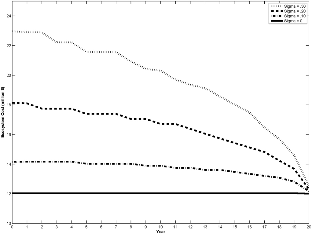
Figure 1. Critical cost (free boundary) curves for different levels of ecosystem cost uncertainty, σ. The curves represent the threshold value of ecosystem costs at which the dam should be removed.

Sensitivity Analysis to Ecosystem Cost Variability, Σ

Figure 1 shows critical cost curves obtained from solving the model using the parameter values in Table 1, but with varying levels of ecosystem cost uncertainty (σ) from 0 to 30 percent. In Figure 1, we observe that variability in ecosystem costs generated by the dam (i.e., σ > 0) increases the critical value at which the dam should be removed. The difference between the curves where ecosystem cost variability exists and the σ = 0 curve is the value of the option associated with delaying dam removal.

TABLE 1

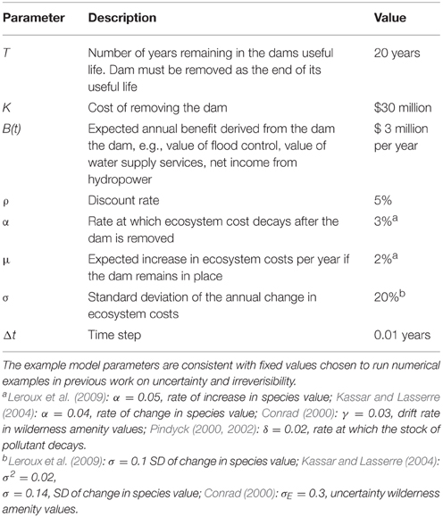
Table 1. Example model parameters.

In Figure 1 all of the critical costs curves, regardless of the magnitude of the ecosystem cost variability, converge to the deterministic critical removal value as the end of the dam's production life is reached. Options decrease in value as the time to maturity approaches, i.e., as the end of the dam's production life is reached. There are two reasons for this. First, the discounted present value of the future benefits (e.g., hydropower, flood control) declines as fewer years of the benefits can be realized. Second, and more important to our discussion of the effects of uncertainty on the dam removal decision, there is less uncertainty regarding the magnitude of the ecosystem costs associated with the dam because the stochastic process describing these costs has less time to drift.

It might seem counter-intuitive that greater ecosystem cost variability prior to dam removal creates an incentive to delay a project intended to restore ecosystem health. However, this is explained by the fact that option values increase with the level of uncertainty, σ. In our model, this means that there is value associated with waiting for more information when the uncertainty is high. The dam removal is irreversible, so there are sunk costs if the dam is removed. Consider that even if ecological costs are high, it is possible that they may decrease as the stochastic ecosystem damages evolve over time -making paying for dam removal avoidable. Meanwhile, if ecological damages move to higher levels, decision-makers can observe this and remove the dam. Hence, additional uncertainty, with the ability to take action, increases the value of waiting. This raises the level of ecosystem cost that society is willing to tolerate before removing the dam relative to the case where ecosystem costs are certain. Of course, though, at some level of cost waiting must cease, and the dam should be removed. This is what the solution to the optimal stopping problem provides—an illustration of the value of delaying a costly ecosystem restoration action. Note that when we incorporate the possibility of jumping to an extreme cost state (e.g., species extinction) in Section Positive Probability of Moving to an Extreme Cost State below, we will observe a countervailing incentive to hasten the action.

Sensitivity Analysis of the Drift Rate (μ)

We specify our model so that ecosystem costs increase stochastically over time as long as the dam remains in place. This is implied by a drift rate parameter, μ, greater than zero (see Equation 3). This drift rate parameter represents the rate at which ecosystem costs increase when the dam is left in place. Figure 2 shows the critical cost curves for several values of μ including the base value in Table 1; all other parameters are held constant at Table 1 values. A higher value of μ shifts the free boundary curve down, i.e., decreases the critical cost at which the dam should be removed. Increasing the drift rate increases the expected rate at which ecosystem costs from the dam accrue. This creates an incentive to remove the dam at an earlier time period. Recall from Section Sensitivity Analysis to Ecosystem Cost Variability, σ and Figure 1 that the critical cost for positive σ converges to the deterministic critical cost at the end of the dam's production life. Figure 2 shows that changing μ causes the deterministic critical cost to shift. For higher μ, it is more valuable to remove the dam at a lower ecosystem cost for any fixed σ. The expected flow of ecosystem cost paid over the next interval of time increases with μ, as does the expected residual costs of the dam. So, higher rates of growth in ecosystem costs imply a lower critical cost that would trigger dam removal.

FIGURE 2

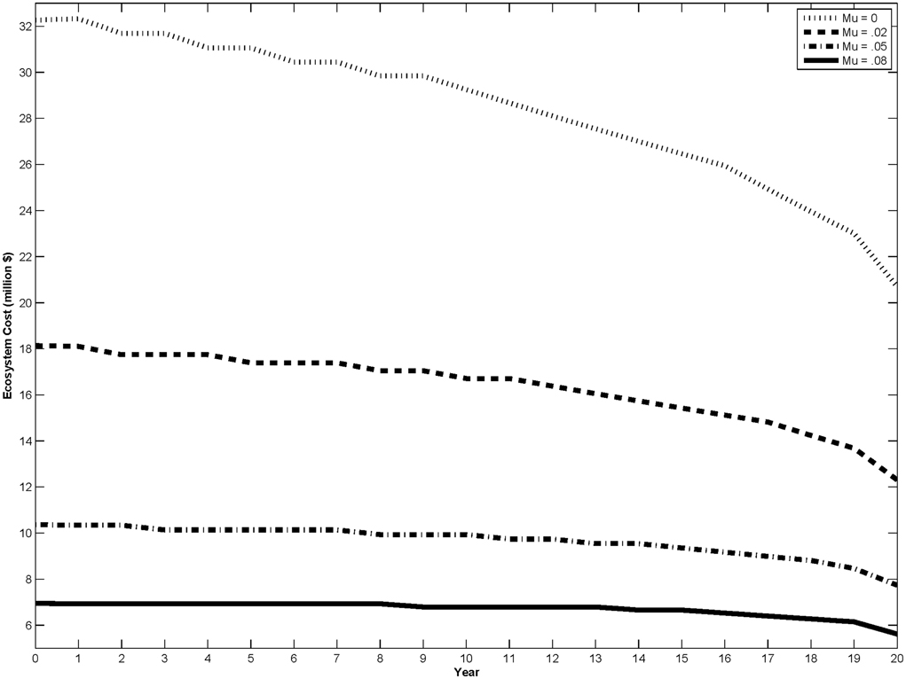
Figure 2. Critical cost curves for different values of the drift rate in ecosystem costs, μ. The curves represent the threshold value of ecosystem costs at which the dam should be removed.

Sensitivity to the Speed of Ecosystem Recovery (α)

The parameter α describes how quickly the ecosystem will recover once the dam is removed and thus determines the value of residual costs. In our model the ecosystem recovers (i.e., ecosystem cost decays) exponentially at a rate of α after the dam is removed. When α is low the ecosystem recovers slowly; when α is high the ecosystem recovers quickly. Figure 3 shows the critical cost curves for different values of α including the Table 1 base value with all other parameters set at Table 1 values.

FIGURE 3

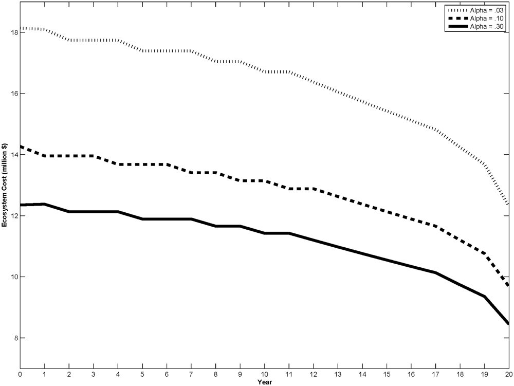
Figure 3. Critical cost curves for different values of the speed of recovery parameter, α. The curves represent the threshold value of ecosystem costs at which the dam should be removed.

Changes in the ecosystem cost decay parameter (α) shift the deterministic critical cost and therefore the point to which positive σ cases converge. The discounted residual costs can be thought of as a lump sum cost that is paid when the dam is removed. Decreasing α increases this lump sum payment because it lowers the rate at which costs decay. The higher the value of this lump sum payment, the greater the benefit to delaying it into the future. According to this model, society is willing to absorb a higher ongoing ecosystem cost when the ecosystem is slow to recover after the dam removal investment (i.e., when residual costs are high) because the present value of the benefit of removing the dam is not as great.

Positive Probability of Moving to an Extreme Cost State

Thus, far we've analyzed the decision of removing the dam under a model of costs changing stochastically according to GBM. While GBM provides a stochastic model for costs, it does not represent the potential outcome of jumping to an extreme cost state—a state that represents extinction or another type of severe event. Under GBM cost uncertainty we found that more uncertainty led to further value in delaying the decision to act. Now we consider that waiting may result in with unacceptably high ecosystem costs.

This risk of irreversible ecological cost is modeled by incorporating a positive probability of jumping to an extreme cost state, C_E (see the jump process in Equation 3). In the example cases below let the extreme cost value C_E = $700 million. To get a sense of the relative size of this number, recall from Figure 1, that the costs where it is optimal to remove the dam are in the region of $10 million. In one of the curves we use the following parameterization of the Gompertz equation, which gives the probability of jumping to an undesirable state (e.g., species extinction):

$\begin{array}{rc}{p}_E(X,b=-\mathit{\text{13}},c=-\mathit{\text{0.004}})=exp\left\{-\mathit{\text{13}}{e}^{-\mathit{\text{0.004X}}}\right\}& (9)\end{array}$

These values and others were chosen to provide an interesting example; in practice they would need to be estimated.

Figure 4 shows the effect of including extinction risk in the model. Incorporating the possibility of jumping to a high cost state causes the free boundary curve to shift down, as shown by the dotted lines in Figure 4. This means that the dam removal is triggered at a lower level of ecosystem costs due to the dam. The additional parameterizations of the jump probability illustrate that any positive probability of jumping to an extreme cost state results in a lower threshold cost. The amount of the shift depends on the parameterization of the jump probability function³. The possibility of jumping to an extreme cost state produces a countervailing incentive to the delay option shown in isolation in Sections Sensitivity Analysis to Ecosystem Cost Variability, σ, Sensitivity Analysis of the Drift Rate (μ), and Sensitivity to the Speed of Ecosystem Recovery (α). While the delay option increases the critical cost to trigger restoration, the possibility of jumping to an extreme cost state decreases the critical cost to trigger restoration. With both of these incentives (delay and hasten) present in the same model, a balance is reached where both the value of waiting for more information and the potential risk of waiting too long are considered.

FIGURE 4

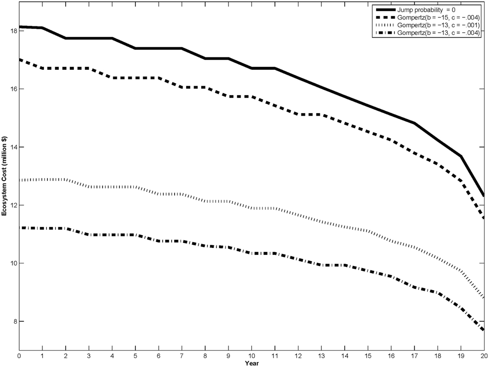
Figure 4. Critical cost curves for different values of the probability of jumping to an extreme cost state. The curves represent the threshold value of ecosystem costs at which the dam should be removed.

Discussion

In this article, we presented a model that incorporates two types of uncertainty that affect the timing of large, irreversible investments in ecosystem restoration: uncertainty regarding stochastically evolving ecosystem costs (geometric Brownian uncertainty) and uncertainty regarding a jump to an unacceptably high level of ecosystem costs (e.g., species extinction). These two uncertainties connect to different irreversible outcomes, sunk costs and permanent ecosystem damage. We use our model to illustrate two main results. First, variability in ecosystem costs creates an incentive to delay a project intended to restore ecosystem health. The uncertainty regarding ecosystem costs creates an option value to waiting to invest in restoration at a later date. Second, the possibility jumping to an irreversible and unacceptably bad ecosystem state creates an incentive to hasten restoration. Many large investments in ecosystem restoration have both characteristics: uncertain ecosystem costs going forward and a risk of outcomes such as species extinction. Therefore, policy makers are faced with countervailing incentives when deciding when to make these investments.

Uncertainty represented by geometric Brownian motion in the evolution of ecosystem costs creates an incentive to delay restoration investments. In our example of dam removal, varying or declining fish populations due to the dam create ecosystem costs that evolve stochastically over time. Policymakers considering dam removal may believe that costs due to poor fish habitat will increase, but this is not a certain outcome. Because dam removal is an irreversible decision, this uncertainty creates an option value which encourages delaying the decision beyond what a deterministic model would show. By contrast, when there is a chance that ecosystem costs can jump to an unacceptably high cost state, an incentive to hasten the restoration investment follows. Policymakers will want to consider each of these countervailing incentives as they make restoration decisions.

Our work applies the result of an option value modeling framework to the important issue of planning for protected species recovery. The results of our work are consistent with previous work that incorporates option value into environmental decision-making, such as pollution prevention investments. Any large, irreversible investment in the presence of uncertain future benefits creates an option value which delays the optimal time of the investment. Similarly, when there is a possibility of moving to an extremely undesirable state, the optimal time of the investment is hastened.

Previous work has applied such models to species extinction problems. That work generally describes the irreversibilty associated with destroying habitat or otherwise reducing the viability of a protected species. Our model, however, specifies investment in an expensive recovery action as the sunk cost. Therefore, we apply the option value framework to a different decision that often faces decision makers: i.e., the best time to spend a large amount of money on recovering a species at risk.

Our model provides a systematic way of understanding the risks and irreversibilities involved in ecosystem management. Clarifying how uncertainty and irreversibility affect the optimal timing of restoration expenditures can be useful as policymakers decide which projects to pursue and in helping to prioritize expenditures and research. Moreover, uncertainty can be reduced by better insight gained through research. Understanding how different uncertainties influence the value of ecosystem restoration decisions can help scientists direct their expertise to research that optimizes the use of funding aimed at ecosystem restoration.

Reaching a potentially extreme cost state is currently an issue in some rivers where Pacific salmon species are listed under the United States Endangered Species Act. Policymakers are currently evaluating large dam removal projects. Our hope is that the dynamic model illustrated here provides insight into making some of these difficult decisions.

Conflict of Interest Statement

The authors declare that the research was conducted in the absence of any commercial or financial relationships that could be construed as a potential conflict of interest.

Acknowledgments

The authors thank Cindy Thomson, Aaron Mamula, Rosemary Kosaka, participants in the 2014 NMFS Protected Resources Economics Workshop, the editor, and the three reviewers for helpful comments. All content is the sole responsibility of the authors.

Supplementary Material

The Supplementary Material for this article can be found online at: https://www.frontiersin.org/article/10.3389/fmars.2015.00101

Figure S1. Illustration of the the cost diffusion in the binomial tree. C₀ is the initial ecosystem cost. C_E is the cost associated with moving to an ecosystem state where restoration is prohibitively costly. C_u and C_d are the potential states that the cost can move to in the next time step under a binomial process.

Footnotes

1. ^Note that we treat benefits, such as hydropower production, deterministically so that our results are focused on ecosystem cost uncertainty.

2. ^A Weiner process is also known as Brownian motion and dz = ε(t)√dt, where ε(t) ~ N(0, 1).

3. ^In general, the b parameter in the Gompertz equation (see Equation 9) shifts the Gompertz curve left and right. The c parameter determines the growth rate of the probability. Using b to shift the Gompertz curve to the right (for example b going from −13 to −15) decreases the chance of jumping to the extreme state for the same value of X. This parameter perturbation moves the critical cost curve up toward the curve where there is a zero probability of jumping to the extreme cost state. Increasing the probability growth rate (parameter c) moves the critical cost curve down. This can be seen in Figure 4 from the example where the growth rate is changed from 0.001 to 0.004 for the same value of b = −13. A full sensitivity analysis involving the jump probability function parameters would be an interesting exercise, but is beyond the scope of this paper. Such an exercise would involve linking these parameters to specific ecological characteristics of the system.

References

American Rivers (2006). Restoring Rivers: Major Upcoming Dam Removals in the Pacific Northwest. Portland, OR: American Rivers.

Bednarek, A. T. (2001). Undamming rivers: a review of the ecological impacts of dam removal. Environ. Manage. 27, 803–814. doi: 10.1007/s002670010189

PubMed Abstract | CrossRef Full Text | Google Scholar

Beechie, T., Buhle, E., Ruckelshaus, M., Fullerton, A., and Holsinger, L. (2006). Hydrologic regime and the conservation of salmon life history diversity. Biol. Conserv. 130, 560–572. doi: 10.1016/j.biocon.2006.01.019

CrossRef Full Text | Google Scholar

Bunn, S. E., and Arthington, A. H. (2002). Basic principles and ecological consequences of altered flow regimes for aquatic biodiversity. Environ. Manage. 30, 492–507. doi: 10.1007/s00267-002-2737-0

PubMed Abstract | CrossRef Full Text | Google Scholar

Connon, R. E., Deanovic, L. A., Fritsch, E. B., D'Abronzo, L. S., and Werner, I. (2011). Sublethal responses to ammonia exposure in the endangered delta smelt; Hypomesus transpacificus (Fam. Osmeridae). Aquat. Toxicol. 105, 369–377. doi: 10.1016/j.aquatox.2011.07.002

PubMed Abstract | CrossRef Full Text | Google Scholar

Conrad, J. M. (2000). Wilderness: options to preserve, extract, or develop. Resour. Energy Econ. 22, 205–219. doi: 10.1016/S0928-7655(00)00031-2

PubMed Abstract | CrossRef Full Text | Google Scholar

Dixit, A. K., and Pindyck, R. S. (1994). Investment Under Uncertainty. Princeton, NJ: Princeton University Press.

Google Scholar

Duke, J. M., Dundas, S. J., and Messer, K. D. (2013). Cost-effective conservation planning: lessons from economics. J. Environ. Manage. 125, 126–133. doi: 10.1016/j.jenvman.2013.03.048

PubMed Abstract | CrossRef Full Text | Google Scholar

Federal Energy Regulatory Commission (2002). Final Supplemental Final Environmental Impact Statement, Condit Hydroelectric Project Washington. FERC Project No. 2342. Available online at: http://digital.library.ucr.edu/cdri/documents/ConditDam_2002_FERCSupplementalFEIS.pdf

Hammitt, J. K. (2013). Positive versus normative justifications for benefit-cost analysis: implications for interpretation and policy. Rev. Environ. Econ. Policy 7, 199–218. doi: 10.1093/reep/ret009

CrossRef Full Text | Google Scholar

Hanley, N. (2001). Cost-benefit analysis and environmental policymaking. Environ. Plann. C 19, 103–118. doi: 10.1068/c3s

CrossRef Full Text | Google Scholar

Kassar, I., and Lasserre, P. (2004). Species preservation and biodiversity value: a real options approach. J. Environ. Econ. Manage. 48, 857–879. doi: 10.1016/j.jeem.2003.11.005

CrossRef Full Text | Google Scholar

Katz, J., Moyle, P. B., Quiñones, R. M., Israel, J., and Purdy, S. (2013). Impending extinction of salmon, steelhead, and trout (Salmonidae) in California. Environ. Biol. Fishes 96, 1169–1186. doi: 10.1007/s10641-012-9974-8

CrossRef Full Text | Google Scholar

Lande, R. (1993). Risks of population extinction from demographic and environmental stochasticity and random catastrophes. Am. Nat. 142, 911–927. doi: 10.1086/285580

CrossRef Full Text | Google Scholar

Leroux, A. D., Martin, V. L., and Goeschl, T. (2009). Optimal conservation, extinction debt, and the augmented quasi-option value. J. Environ. Econ. Manage. 58, 43–57. doi: 10.1016/j.jeem.2008.10.002

CrossRef Full Text | Google Scholar

Ligon, F. K., Dietrich, W. E., and Trush, W. J. (1995). Downstream ecological effects of dams. Bioscience 45, 183–192. doi: 10.2307/1312557

CrossRef Full Text | Google Scholar

McElhany, P., Ruckelshaus, M., Ford, M. J., Wainwright, T., and Bjorkstedt, E. (2000). Viable Salmonid Populations and the Recovery of Evolutionarily Significant Units. Seattle, WA: U.S. Department of Commerce; NOAA Technical Memorandum NMFS-NWFSC-42; Northwest Fisheries Center.

Google Scholar

Medellín-Azuara, J., Durand, J., Fleenor, W., Hanak, E., Lund, J., Moyle, P., and Phillips, C. (2013). Costs of Ecosystem Management Actions for the Sacramento-San Joaquin Delta. San Francisco, CA: Public Policy Institute of California.

Google Scholar

National Park Service (2005). Elwha River Ecosystem Restoration Implementation: Final Supplement to the Final Environmental Impact Statement. Port Angeles, WA: National Park Service; U.S. Department of the Interior; Olympic National Park. Available online at: http://www.nps.gov/olym/naturescience/elwha-restoration-docs.htm

Parker, A. E., Dugdale, R. C., and Wilkerson, F. P. (2012). Elevated ammonium concentrations from wastewater discharge depress primary productivity in the Sacramento River and the northern San Francisco Estuary. Mar. Pollut. Bull. 64, 574–586. doi: 10.1016/j.marpolbul.2011.12.016

PubMed Abstract | CrossRef Full Text | Google Scholar

Pearce, D. (1998). Cost benefit analysis and environmental policy. Oxf. Rev. Econ. Policy 14, 84–100. doi: 10.1093/oxrep/14.4.84

CrossRef Full Text | Google Scholar

Pess, G. R., McHenry, M. L., Beechie, T. J., and Davies, J. (2008). Biological impacts of the Elwha River dams and potential salmonid responses to dam removal. Northwest Sci. 82, 72–90. doi: 10.3955/0029-344X-82.S.I.72

CrossRef Full Text | Google Scholar

Pindyck, R. S. (2000). Irreversibilities and the timing of environmental policy. Res. Energy Econ. 22, 233–259. doi: 10.1016/S0928-7655(00)00033-6

CrossRef Full Text | Google Scholar

Pindyck, R. S. (2002). Optimal timing problems in environmental economics. J. Econ. Dyn. Control 26, 1677–1697. doi: 10.1016/S0165-1889(01)00090-2

CrossRef Full Text | Google Scholar

Pringle, C. (2003). What is hydrologic connectivity and why is it ecologically important? Hydrol. Process. 17, 2685–2689. doi: 10.1002/hyp.5145

CrossRef Full Text | Google Scholar

Portland General Electric (2002). Decommissioning Plan for the Bull Run Hydroelectric Project. FERC Project No. 477. Filed by Portland General ElectricCompany with the Federal Energy Regulatory Commission Office of Hydropower Licensing. Available online at: http://web.archive.org/web/20070928065333/http://www.portlandgeneral.com/about_pge/news/sandy_land/decommissioning_plan.pdf

Saphores, J. D. (2003). Harvesting a renewable resource under uncertainty. J. Econ. Dyn. Control 28, 509–529. doi: 10.1016/S0165-1889(03)00033-2

CrossRef Full Text | Google Scholar

Saphores, J. D., and Shogren, J. F. (2005). Managing exotic pests under uncertainty: optimal control actions and bioeconomic investigations. Ecol. Econ. 52, 327–339. doi: 10.1016/j.ecolecon.2004.04.012

CrossRef Full Text | Google Scholar

US Bureau of Reclamation (2012a). Benefit Cost and Regional Economic Development Technical Report for the Secretarial Determination on Whether to Remove Four Dams on the Klamath River in California and Oregon. Denver, CO: Bureau of Reclamation Technical Services Center. Available online at: http://klamathrestoration.gov/sites/klamathrestoration.gov/files/2013%20Updates/Econ%20Studies%20/f.BCA_7-20-2012%20(accessible).pdf

US Bureau of Reclamation (2012b). Hydropower Benefits Technical Report for the Secretarial Determination on Whether to Remove Four Dams on the Klamath River in California and Oregon. EC-2011-02. Denver, CO: Bureau of Reclamation Technical Services Center. Available online at: http://klamathrestoration.gov/sites/klamathrestoration.gov/files/2013%20Updates/Econ%20Studies%20/i.Hydropower_7-17-2012_Accessible.pdf

Verbruggen, A. (2013). Revocability and reversibility in societal decision-making. Ecol. Econ. 85, 20–27. doi: 10.1016/j.ecolecon.2012.10.011

CrossRef Full Text | Google Scholar

Washington State Department of Ecology (2007). Condit Dam Removal Final SEPA Supplemental Environmental Impact Statement (FSEIS). Publication number 07-06-012. Available online at: https://fortress.wa.gov/ecy/publications/publications/0706012.pdf

Wu, J. J., Adams, R. M., and Boggess, W. G. (2000). Cumulative effects and optimal targeting of conservation efforts: steelhead trout habitat enhancement in Oregon. Am. J. Agric. Econ. 82, 400–413. doi: 10.1111/0002-9092.00034

CrossRef Full Text | Google Scholar

Wu, J. J., and Skelton-Groth, K. (2002). Targeting conservation efforts in the presence of threshold effects and ecosystem linkages. Ecol. Econ. 42, 313–331. doi: 10.1016/S0921-8009(02)00104-0

CrossRef Full Text | Google Scholar