Assessing the Role of Environmental Factors on Baltic Cod Recruitment, a Complex Adaptive System Emergent Property
 Dionysis Krekoukiotis
 Artur Piotr Palacz
 Michael A. St. John
- DTU Aqua, National Institute of Aquatic Resources, Technical University of Denmark, Charlottenlund, Denmark
For decades, fish recruitment has been a subject of intensive research with stock–recruitment models commonly used for recruitment prediction often only explaining a small fraction of the inter-annual recruitment variation. The use of environmental information to improve our ability to predict recruitment, could contribute considerably to fisheries management. However, the problem remains difficult because the mechanisms behind such complex relationships are often poorly understood; this in turn, makes it difficult to determine the forecast estimation robustness, leading to the failure of some relationships when new data become available. The utility of machine learning algorithms such as artificial neural networks (ANNs) for solving complex problems has been demonstrated in aquatic studies and has led many researchers to advocate ANNs as an attractive, non-linear alternative to traditional statistical methods. The goal of this study is to design a Baltic cod recruitment model (FishANN) that can account for complex ecosystem interactions. To this end, we (1) build a quantitative model representation of the conceptual understanding of the complex ecosystem interactions driving Baltic cod recruitment dynamics, and (2) apply the model to strengthen the current capability to project future changes in Baltic cod recruitment. FishANN is demonstrated to bring multiple stressors together into one model framework and estimate the relative importance of these stressors while interpreting the complex non-linear interactions between them. Additional requirements to further improve the current study in the future are also proposed.
Introduction
Natural living systems are characterized by a high level of complexity, which results from the diversity of their biological components and from the diversity of possible types of interaction (physical, chemical, trophic, behavioral, cognitive; Planque et al., 2014). Many biological interactions are non-linear and biological systems display a remarkable ability to constantly adapt and reconfigure themselves (Planque et al., 2014). Such systems, including marine ecosystems, are characterized by multiple possible outcomes and by the potential for rapid changes and ecological surprises (Doak et al., 2008; Levin and Lubchenco, 2008; Scheffer, 2009; Glaser et al., 2011; Möllmann et al., 2011). This display of high complexity, non-linearity, and adaptability has identified these systems as Complex Adaptive Systems (CAS, Levin, 2005).
For decades, fish recruitment has been a matter of intensive research (e.g., Ricker, 1954; Cushing, 1971; Rothschild, 2000) and is recognized as a key element in management decisions (Fernandes et al., 2015). Models of stock–recruitment (e.g., Ricker, 1954; Beverton and Holt, 1957; Cushing, 1996) commonly used for recruitment prediction often explain only a minor fraction of the inter-annual variation in recruitment. This lack of predictive strength has been assumed to be explained by the influence of different factors in the environment (O'Brien and Little, 2006; Margonski et al., 2010). Consequently, this research area has evolved from considering simply the spawning stock biomass (SSB), to include also use of environmental factors and relationships that can modulate recruitment (Köster et al., 2005; Schirripa and Colbert, 2006). Presently, stock recruitment models along with other regression methods including environmental variables (Planque and Buffaz, 2008), are commonly used for recruitment prediction (Fernandes et al., 2010). This use of environmental information to improve the ability to predict recruitment, could contribute considerably to fisheries management (De Oliveira et al., 2005; Yuan et al., 2012).
A large number of studies have been undertaken using different techniques, to utilize such environmental information to predict recruitment (e.g., Chen and Ware, 1999; Bailey et al., 2005; Dreyfus-León and Chen, 2007; Dreyfus-León and Schweigert, 2008; MacKenzie et al., 2008; Ruiz et al., 2009). Nevertheless, the recruitment problem remains difficult because the mechanisms behind such complex relationships are often poorly understood; this in turn leading to the failure of some proposed relationships, methods, and performance estimations, when new data become available (Myers et al., 1995). Such failures may be related to new controls, which were not previously considered (Myers et al., 1995; Planque and Buffaz, 2008), or to limitations of the available data (Schirripa and Colbert, 2006).
The Baltic Sea has been studied extensively and is identified as being a region of rich data with extensive time series from environmental and biological monitoring (Eero et al., 2015). It is an ecosystem that “has been and will continue to be impacted by various stressors including climate change, exploitation, and eutrophication” (MacKenzie et al., 2012). During the last three decades, it is hypothesized that the Baltic has undergone a regime shift, altering the functioning and structure of its zooplankton and fish communities. The new stable state has been considered as “cod hostile” (e.g., Möllmann et al., 2008, 2009; Lindegren et al., 2010) due to reduced spawning success in cod, owing to adverse hydrological conditions as well as increased predation on cod eggs and declining food resources for cod larvae (Casini et al., 2009).
Several changes in the biological parameters of Baltic cod, managements and fisheries have occurred in recent years, all of which could have potentially had a positive influence on the development of the stock (Eero et al., 2012). However, there was a fail in the analytical stock assessment in 2014, leaving unclear the present stock status. Changes in ecological and environmental conditions have led to an unusual situation for Baltic cod and it has been suggested that the stock is “in distress” (Eero et al., 2015). Clearly, the recruitment dynamics of Baltic cod are “more complex than previously thought” (Köster et al., 2005), thus, our understanding in the status of cod in the Baltic Sea and efforts in solving stock assessment and recruitment issues is “ongoing and will likely continue in the coming years” (Eero et al., 2015).
The current conceptual model of the understanding of Baltic cod recruitment dynamics is given by Köster et al. (2003) and Köster et al. (2005), and references therein. “Hydrographic conditions in the central Baltic were affected by large-scale climatic conditions during the 80s and 90s, resulting in higher than normal temperatures in the intermediate and bottom water and declining salinity and oxygen concentrations in the deep Baltic basins” (Köster et al., 2005). Reproductive success of the top-predator cod declined and “anoxic conditions in deep layers at important spawning sites caused severe egg mortalities” (Köster et al., 2005). The observed recruitment decline of the 1980s was believed to be related to these “climate-induced changes in the physical environment” (Köster et al., 2005). Herring stock sizes and especially sprat, important planktivorous predators and in the case of sprat a key predator on cod eggs, increased substantially. Furthermore, “a temperature-related increase in the sprat stock intensified egg predation” (Köster et al., 2005).
Even though the hydrographic conditions facilitative for survival of early life stages improved during the 90s, cod recruitment success remained far below average. The lack of recruitment recovery in the mid-90s, “despite improved hydrographic conditions for egg development, is related to poor larval survival” (Köster et al., 2005) and cod egg predation (Köster and Möllmann, 2000; Casini et al., 2009). A decline in the abundance of the copepod Pseudocalanus sp. (Möllmann et al., 2008) related to lower salinity and increased predation by clupeid fish, mainly sprat (Casini et al., 2009), caused food limitation for first-feeding cod larvae. Few exceptions in recruitment in the 90s have been suggested to be due to relatively high wind speeds (affecting transport and prey encounter via turbulence), and below average temperatures, favoring oxygen conditions for egg survival.
It has long been recognized that non-linear population processes and environmental forcing can generate dramatic fluctuations in recruitment of marine fish and invertebrate stocks (Glaser et al., 2011; Mäntyniemi et al., 2015). It is difficult to clarify and model the mechanisms controlling recruitment by using conventional methods because fish populations have complex and non-linear response, and reactions to biotic inter-reactions and environmental changes (Olden and Jackson, 2001). Machine-learning techniques such as Artificial Neural Networks (ANNs) have been proposed as “an appropriate approach with some desirable properties to address such problems” (Dreyfus-León and Chen, 2007; Uusitalo, 2007; Fernandes et al., 2013). ANNs gained momentum in mid-1980s (Rumelhart et al., 1986) and subsequently they have been used in a variety of ecological applications. ANNs mimic biological neural networks to fit and find patterns in complex data (Lawrence, 1993). For a more comprehensive treatment of ANN applications in ecology, we suggest the books by Lek and Guegan (2000), Lek et al. (2005), and Recknagel (2006).
ANNs have been shown to approximate competently many complex functions and have demonstrated advantages in predictive ability over general linear models (Hastie et al., 2001). In many cases they are documented to perform better than multiple regressions when there are non-linear relationships between the variables (Lek et al., 1996; Brey et al., 1997). Their main advantage compared with multiple regression models is that they do not require an a priori model as they can learn from existing data. Additionally, ANNs can model systems that involve complex non-linear relationships between variables and outcomes multiple dependent variables, can learn from “noisy data” (Kasabov, 1996) and the outputs of the multi-layer perceptron (MLP), a type of ANN, can be interpreted as “probabilities” (Watts and Worner, 2008). They can generalize well if over-fitting is avoided, in other words they can fit and classify data they have not been trained on with accuracy. They also do not require the transformation of non-linear variables, unlike classical linearization techniques, which can “improve the results but have often failed to fit the data” (Sun et al., 2009). All these features make the application of ANNs “a powerful approach for exploring complex biological problems such as recruitment forecasting” (Chen and Ware, 1999).
This utility of neural networks for solving non-linear problems has been demonstrated in aquatic studies and has led many researchers to comment on neural networks as an attractive (non-linear) alternative to traditional statistical methods (Olden and Jackson, 2002). A thorough revision of the use of neural networks in fisheries research was performed by Suryanarayana et al. (2008) where applications in forecasting, fisheries management distribution and classification since 1978 where reviewed. In addition, Quetglas et al. (2011) also reviewed the utilities of neural networks in marine ecology and fisheries science during the 1990s and 2000s. Some interesting applications of ANN to management and forecasting of fisheries include the modeling of recruitment, stock biomass, abundance, catch of different fisheries, and distribution (Komatsu et al., 1994; Lek et al., 1996; Mastrorillo et al., 1997; Chen and Ware, 1999; Laë et al., 1999; Chen et al., 2000; Gevrey et al., 2003; Maravelias et al., 2003; Zhou, 2003; Joy and Death, 2004; Chen and Hare, 2006; Glaser et al., 2011; Olden et al., 2011; Russo et al., 2011, 2014).
Many published works on ANNs in marine ecology compare this approach with classical multivariate statistical methods, such as multiple linear regression (MLR) or discriminant analysis (DA). Quetglas et al. (2011) state that in all cases, ANNs either outperformed (e.g., Baran et al., 1996; Lek et al., 1996; Mastrorillo et al., 1997; Laë et al., 1999; Ibarra et al., 2003; Wagner et al., 2006) or at least performed as well (e.g., Power et al., 2005; Fang et al., 2009) as classical linear and non-linear modeling methods, such as linear regression and generalized additive models with respect to prediction accuracy.
There are only two publications in literature that have applied ANNs in studies on Baltic cod. Wieland and Jarre-Teichmann (1997) used an artificial neural network model to successfully predict the vertical distribution of Baltic cod eggs. Fuchs (1996) utilized ANN as a tool to investigate how the changed hydrography influences the cod distribution in the Baltic. To our knowledge, ANNs have not been applied to investigate recruitment of Baltic Cod. Thus, the goals of this study were to (1) build a quantitative model representation of the conceptual understanding of the complex ecosystem interactions driving Baltic cod recruitment dynamics, and (2) apply the model to strengthen the current capability to project future changes in Baltic cod recruitment.
Materials and Methods
Data Sources
The data utilized cover the ICES subdivisions 25, 26, and 28-2 in the Baltic Sea (Figure 1), thus encompassing the three major basins known as nursery grounds of eastern Baltic Cod. Here, we analyze biotic and abiotic information as combined time series from all three subdivisions, assuming little effect of transport between spawning areas (Köster et al., 2005). Cod Reproductive Volume from May to August (RVmay, RVaug) were calculated and applied separately as the water column volume with salinity above 11 and dissolved oxygen above 2 ml/l, i.e., proper conditions ensuring fertilization and egg development of cod (Plikshs, 2014). Datasets where obtained from M. Plikshs (Fishery Resources Research Department, Riga, Latvia) and B.R. Mackenzie (Technical University of Denmark, Charlottenlund, Denmark). The effects of natural and fishing mortality (i.e., survival and harvest) were considered variable over time. Natural and Predation Mortality parameters (NatMort) at Age 2 of Cod, are basin-wide estimates derived from the Stochastic Multispecies Model (SMS), a data-driven model frequently used for generating analytical fish stock assessments and forecasts as basis for ICES scientific advice (Lewy and Vinther, 2004). Fishing mortality (FishMort) and SSB estimates are derived from published ICES stock assessments (ICES, 2010).
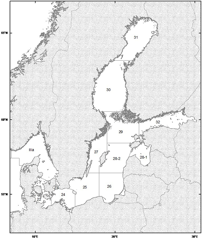
Figure 1. Map of ICES Statistical area for the Baltic Sea (http://ices.dk/marine-data/maps/Pages/default.aspx). Courtesy of International Council of the Exploration of the Sea.
As an estimate of recruitment we used the number of cod recruits to the fishery at an age of 2. Earlier estimates of year-class strength are difficult to assess due to cannibalism effects (Köster et al., 2003). As a result, regular single species assessments of cod employ Age-2 as the youngest age group and presentations of stock-recruitment relationships refer in general to age-group 2 (Köster et al., 2003) as the first age fully recruited to and sampled by the fishery. Abundance index of Age-2 Baltic Cod is derived from published ICES stock assessments and was used as an estimate of the number of cod recruits to the fishery (Köster et al., 2003). Additionally, we consider habitat driven variables, proposed by Köster et al. (2005), that potentially explain changes in recruitment regimes, namely: Oxygen—related Egg Survival (OES), Relative egg Predation Pressure (RPP), Egg abundance (EA), and Larval Abundance (LA; Köster et al., 2005). We obtained the published 1976–1999 time series of these variables from Köster et al. (2005). Information on the variables employed in this study including duration of time series and data source are presented in Table 1. Additionally, 2000–2009 data time series were used as independent test sets to assess the predictive accuracy of those models for which all input and target variables were available during this period (also presented in Table 1). Time series plots for the 9 input variables and cod at Age-2 are presented in Figure 2.
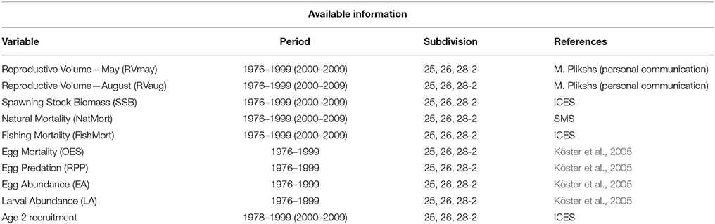
Table 1. List of variables applied to the models.
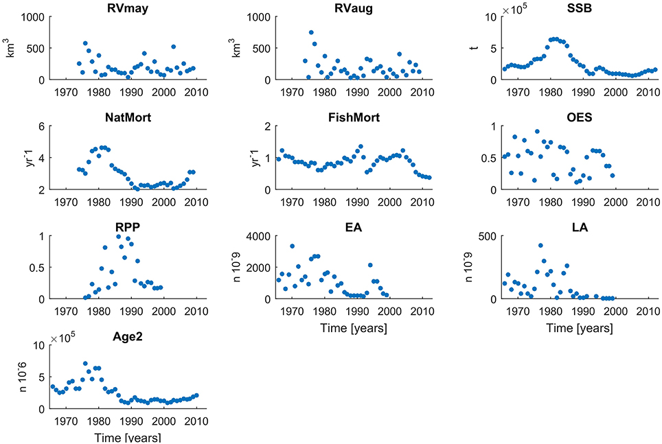
Figure 2. Time series of all input and target variables used to build the FishANN model in different configurations.
In order to enable a potential operational 2-year-ahead forecast of eastern Baltic cod recruits we only consider model input variables available 2 years ahead of the estimated recruit abundance. For habitat driven variables and SSB this is representative of their direct influence on the earliest life stages of the cod (eggs and larvae). In case of natural and fishing mortality here we use a sum of the given mortality term on cod age 0, 1, and 2 from 2years back with respect to the given cod Age-2 recruit abundance estimate. While these indices do not match the conceptual direct influence these variables have on cod recruitment to the fishery in a given year, they nevertheless explain a large part of the target variable variability. This approach is deliberately different from a typical analytical stock assessment model procedure, which would replace the in-year natural and fishing mortality estimates with the average from last few years as proxies for these variables, when running the models in forecast mode.
Modeling Approach
In terms of structure, ANNs are non-linear models that apply weighted links between input neurons (predictors), hidden neurons, and output neurons (results) related to a response. Training any type of supervised ANN consists of using a response training dataset to adjust the connection weights in order to minimize the error between observed and predicted response values. These weights are the parameters of ANNs, initially chosen from random numbers and are refined until convergence or maximum clock time set is over. In feed-forward networks, neurons from one layer are interconnected to all neurons of neighboring layers, but no connections are established within a layer or feedback connection. After being trained to match inputs and response outputs with existing data, an ANN can be used for forecasting with new inputs.
We use feed-forward neural networks, with a single hidden layer, trained in supervised mode using the back propagation algorithm (Rumelhart et al., 1986). The modeling process in back-propagation neural networks is more direct, as there is no necessity to specify a mathematical relationship between the input variables and output responses (Goh, 1995). This category of neural networks, referred to as MLPs, is commonly used in ecological studies as MLPs are suggested to be universal approximators of any continuous function (Hornik and White, 1989; Olden et al., 2004). The MLP was first used in ecological studies in fisheries in Komatsu et al. (1994) and Lek et al. (1995), and since then has been successfully applied to several different problems in ecology (Kimes et al., 2000; Quetglas et al., 2011). In our study, calculations were done in the MathWorks Matlab environment using the Neural Networks Toolbox.
Model Training and Testing Procedure
The MLP neural network models we used are trained via Bayesian regularized method (BR) using MATLAB's native “trainbr” function. BR training tends to show better performance when the relationship between variables is non-linear (Sovan et al., 1996; Archontoula et al., 2003). It also gives potentially better generalizations because of its capability to automatically select regularization parameters to optimize the network architecture and limit the likelihood of over-fitting (Burden and Winkler, 1999, 2000). We chose the estimated mean of squared errors (MSE) as the representative metric of performance of the model. The smaller the MSE, the better the model fit. To further minimize the risk of over-fitting the model, a validation stop criterion was introduced to the BR training function, hence the model training stopped as soon as it failed to minimize its error for n-number consecutive training cycles, here n = 20 (e.g., Sjöberg, 1995; Amari et al., 1997).
To further avoid overtraining and to maximize generalizability (i.e., ability to project correctly in unsupervised mode) three-fold cross-validation was used to assess model prediction accuracy, meaning that 1/3 of all available data points from the 1976–1999 input time series were always excluded from training a given set of models. In the training set the data was further divided randomly for training and validation (70 and 30%, respectively) with a different random split for each model. The training data set was used to iteratively adjust the connection weights until a minimum error was found. The validation data set was used to monitor network error after each training cycle, enabling training to be terminated when the network began to over-train or over-fit the data. We compared the test set performances from the three-fold cross-validation and selected the model with the best of the three test set MSEs.
Model Ensemble
Stochasticity needs to be considered as an important trade-off when using data-driven approaches such as ANNs. In order to account for the variability in model results, dependent on the initial choice of weights and random data splitting during training, we employed an ensemble model approach similar to the suggestions discussed in Zhou (2003), and De Oña and Garrido (2014). For each training data set we trained an N-number of replicate models (herein N = 35), with identical architecture (see Section Model Ensemble) but different set of initial weights. The performance of the given ensemble member model (m#; # = 1, 2, …, 35) was estimated on the test set through a cross-validation procedure described above. The ensemble model performance was considered equal to the median of all 35 replicate models.
To test the hypothesis that the larger the number of ensemble members, the higher the performance of the ensemble, we performed a sensitivity experiment, the results of which are presented in Figure 3. In this analysis we checked the test set performance of each ensemble and plotted the MSE of the ensemble best model as a function of the number of ensemble members ranging from 1 to 90, again applying three-fold cross-validation as above. Each ensemble configuration was run with 10 replicates, and only the median of the 10 results was plotted in Figure 3.
Figure 3. Test set MSE of the best model within an ensemble as a function of the number of ensemble members. The results displayed are the median of 10 replicates performed for each number of ensemble members. All results obtained while applying the three-fold cross-validation procedure for every model. Red line shows the results from choosing the best of the three-folds, black line—median of the three-folds, blue line—mean of the three-folds, for each individual ensemble member model.
We found that there is a marked and consistent increase in performance (decrease in MSE) of the ensemble best as the number of ensemble members increased from 1 to around 10 to 15. However, no consistent and significant gain in performance could be achieved when increasing the number of ensemble members beyond the number 35. Figure 3 also illustrates that this result does not depend on whether we select the best, the mean or the median of the three-folds during cross-validation when used to report the performance of each individual ensemble members. While the absolute value of the ensemble MSE changes, all three lines show little if any gain in ensemble performance beyond 35 ensemble members.
Model Architecture
The general architecture of the neural network model used in this study is the same, i.e., there is one input layer, one output layer, and a single so-called hidden layer with three computing units (neurons). The number of neurons was set to three, optimized based on the results of sensitivity analysis performed according to the following procedure. Using a number of neurons in the range from 1 to 30 we trained 20 nets with 9 input variables for every number of neurons and recorded their average (mean and median) performance (MSE criterion), both on training and test sets (Figure 4). The 20 nets differed in terms of their initial weights and distribution of training and test set on the 1976–1999 input time series. The mean of the 20 replicates revealed no consistent trends but the median results from 20 replicates revealed that while training errors kept decreasing until the number of neurons reaches 7 and then showed little if any change, the median test set error reached a global minimum already at three neurons in the hidden layer. Therefore, we opted for the MLP model configuration with the simplest architecture and highest generalization capability, i.e., with three neurons in the hidden layer.
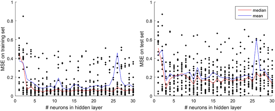
Figure 4. Test and training set MSE as a function of the number of neurons in the hidden layer. The results displayed are the mean and median of 20 replicates performed for each number of neurons in the hidden layer, evaluated separately for the training set (Left panel) and the test set (Right panel).
Input Layer Structure—Feature Selection
For the purpose of designing an optimal model capable of predicting eastern Baltic cod recruits 2-years ahead we constructed a series of MLP neural networks that differ from each other by the number of input variables considered, on a range from one to nine. In order to reduce the number of potential input variable combinations we used a quantitative feature selection method based on the results of variable importance analysis, described in detail below. Additionally, we adopted a qualitative criterion which restricted the number of potential input variables to five, which had available data points from the entire time period under study (RVmay, RVaugust, SSB, NatMort, FishMort). Therefore, feature selection was applied independently on two original models: MLP1—with nine input variables, and MLP2—with five input variables. Based on the results of feature selection analysis, which discarded those variables whose importance was significantly lower than others based on the median variable importance from the MLP ensemble, we then identified and retrained two new models with a reduced number of input variables (MLP3 and MLP4). Performance of reduced models was compared to the original ones with a full feature suite. Finally, we include one more model into the analysis with only a single input variable SSB (MLP5), thus mimicking the simplest possible stock-recruitment relationship model.
Variable importance-based feature selection was performed using two metrics derived from the distribution of connection weights inside a trained model: (i) product-of-standardized-weights (PSW) first defined in Garson (1991) and as applied in Russo et al. (2011), and (ii) product-of-connection-weights (PCW) based on Olden and Jackson (2002) and Olden et al. (2004). Measures of variable importance for both methods were obtained using MATLAB code. The two approaches are briefly described below. For full documentation we refer to the publications mentioned above.
In the PSW method the algorithm partitions hidden-output connection weights into components associated with each input neuron using absolute values of connection weights. It is important to note that Garson's PSW algorithm uses the absolute values of the connection weights, thus the variable contributions cannot reveal anything about the direction of the relationship between the input and output variables. The PCW approach of Olden and Jackson (2002) calculates the product of the raw input-hidden and hidden-output connection weights between each input neuron and output neuron and sums the products across all hidden neurons. According to Olden et al. (2004), the application of Garson's algorithm may often be inadequate because using absolute connection weights does not account for counteracting connection weights in cases where there are opposite directions for incoming and outgoing weights from the hidden layer neurons. Therefore, when the two metrics revealed contrasting variable importance ranks, we base our judgments on the PCW approach.
Table 2 lists all the models considered in this study, both before and after the qualitative feature selection.
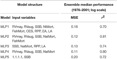
Table 2. Different model structures and their recorded performance.
Results and Discussion
Feature Selection Analysis
Results of the feature selection process based on input variable importance analysis are presented in Figure 5. Using two different algorithms to estimate the neural network connection weights associated with individual input variables, we arrived at similar conclusions as to which features (input variables) are potentially redundant in the two models which use the maximum number of available input variables for either the 1976–1999 training period (MLP1) or the entire time period under study (1976–2009). Both the PCW and the PSW methods applied to the MLP1 ensemble showed on average the lowest importance given to: RVmay, RVaug, FishMort, OES, and EA. According to the PSW method neither of these variables passed a 10% relative importance in determining the model output, taken as the mean of all ensemble members. NatMort and RPP were ranked as the most important variables with LA and SSB values also reaching above 10% on average across all ensemble members. NatMort and RPP were also the variables with highest average connection weights according to the PCW method, which additionally revealed the opposing direction of influence of these two variables—observation not possible to make with the PSW approach. Here, the connection strength of SSB and LA only slightly exceed the average weights assigned to connections traced back to the two RV variables, FishMort, OES, and EA. Based on these results, we reduced the feature space of MLP1 to four input variables with highest average connection weights (SSB, NatMort, RPP, and LA) which then determined the structure of the new model MLP3. Figure 5 also shows the results of variable importance analysis on MLP3. We observed that RPP and NatMort retained their highest relative variable importance, with SSB showing a consistently lower importance relative to the other inputs when compared to MLP1.
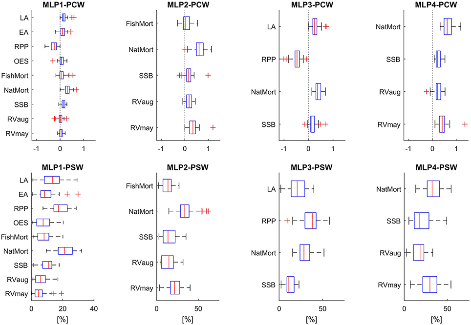
Figure 5. Variable importance based on the PCW and PSW algorithms, for all 5 MLP models. Box plots show the distribution of connection weights within each ensemble member providing a variable importance metric for all model inputs. Red lines mark the median weights, boxes are 75% percentiles, whiskers 2 standard deviations, and red crosses mark the outliers. Top panels show the results obtained using the PCW algorithm, with connection weights in absolute values. Bottom panels show the results obtained using the PSW algorithm, with variable importance given in %.
Analysis of connection weights in the MLP2 model ensemble confirmed the high relative importance of NatMort. The second most important variable, according to both the PCW and PSW algorithms, was RVmay. According to the PCW results, FishMort showed no consistent direction of influence on the model output and displayed the weakest average connection with the output. Consequently, we decided to rule out only this variable when reducing the feature space of MLP2 for the purpose of building the MLP4 model. As in the case of MLP3, the reduction of the feature space did not alter the relative weight distribution significantly. NatMort and RVmay were retained as the most influential variables for determining the model outputs.
In Section Model Performance Evaluation, we further analyze the effects of our feature selection analysis on model performance in order to choose the optimal FishANN MLP configuration.
Model Performance Evaluation
In Table 2 we compared the performance of the five MLP models using two statistical metrics: MSE and squared correlation of determination coefficient (r2). Please note that both the MSE and r2 values reported here represent the ensemble median model performance on those samples from the 1976 to 2001 time-series for which there was a complete suite of input variables available. In terms of MSE the best performance was provided by the MLP4 ensemble, although the improvement over MLP2 was marginal. While the r2 of MLP4 was in fact 0.01 lower than that of MLP2, we must bear in mind that r2 also likely increased due to a mere increase in the number of features. To test that, we calculated the adjusted r2 of MLP4 (0.75) which turned out slightly higher than that of MLP2 (0.74). These results suggest that the variable importance-based feature selection performed on MLP2 led to an improvement in the model performance in form of MLP4.
Reducing the number of features in the MLP1 model resulted in an even more pronounced improvement in the model performance in terms of MSE and r2. Nonetheless, the improved model MLP3 was found to have a lower overall performance than MLP2. It is interesting that the most complex model with nine input variables (MLP1) had a lower r2 than the simplest stock-recruitment model with only SSB in its feature space (MLP5). Reducing the feature space of MLP1 led to MLP3 with an r2 above that of MLP5, however, with an adjusted r2 (0.67) still lower than that of MLP5 (0.70).
These observations and conclusions were additionally confirmed by the results displayed in the Taylor diagram (Figure 6), which shows a more comprehensive multi-statistical analysis of the differences in performance between the five models. Considering not only the correlation of determination coefficient r, but also the central root mean square difference (RMSD) and standard deviation patterns relative to the ICES data. While the differences in terms of correlation and RMSD are narrow between all models, and small gains in reducing the feature space from MLP1 to MLP3, and MLP2 to MLP4, there is an increase in the standard deviation exhibited by the reduced models, with MLP3 standard deviation being in fact the closest to the ICES reference value.
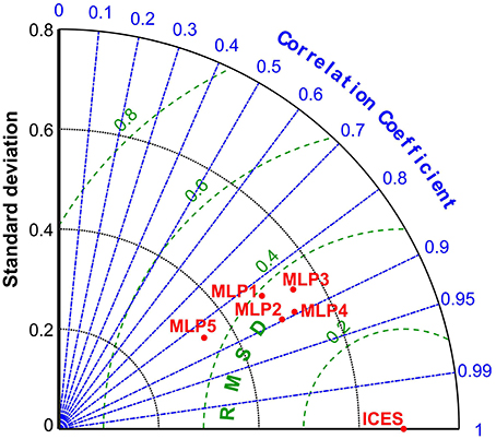
Figure 6. Taylor diagram for multi-statistic model performance evaluation of the 5 MLP models in comparison to the ICES Age-2 numbers reference. RMSD—centered root mean square difference which is a variation of the mean square of errors used to train the MLP models. Correlation of determination here equivalent to the square root of r2 reported in Table 2. Standard deviation and RMSD units expressed on log scale.
In comparison with previous Baltic cod recruitment models in similar studies, Köster et al. (2003) tested existing environmentally sensitive stock-recruitment relationships (Köster et al., 2001) and performed linear regressions of cod recruitment (in numbers) on SSB, using cod Age 2 dependent variables per subdivisions 25, 26, and 28 (R2 = 0.16, R2 = 0.23, and R2 = 0.41, respectively). Röckmann et al. (2007) presented a linear regression of the spawning stock size in time series 1976–1999, with combined model estimates that “explained 72% of the variance of ICES standard stock assessment estimates.” In this approach, recruitment refers to 0 group cod (Age 0). Margonski et al. (2010) demonstrated two different models in their model comparisons for the Eastern Baltic Cod stock: a linear and additive model (R2 = 0.73) and a linear and polynomial model (R2 = 0.725). We assume that the authors considered Age-2 cod as recruiting to the fishery, although this was not stated in the paper.
Time-series comparison of MLP-derived and ICES-based Age-2 numbers estimates displayed in Figure 7 provide also additional information: (a) how well the different ensemble median MLPs perform in the distinct high and low recruitment regimes, and (b) what is the level of uncertainty due to picking any random ensemble member model projection, here defined as the range of variability around the median within each ensemble model.
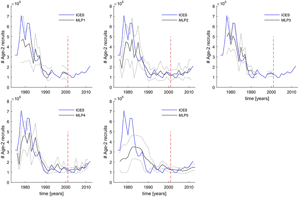
Figure 7. 1976–2011 time-series predictions of five different FishANN MLP structures compared to the ICES number of Age-2 recruits. Gaps in prediction time series are caused by missing input variables at those years. Solid blue lines—ICES reference values in numbers of individuals. Solid black lines are the MLP ensemble model median predictions. Dotted black lines mark the confidence intervals of the MLP predictions equivalent to ±2 standard deviations of the predictions from all 35 ensemble members. The dashed red vertical line separates the time period used for every MLP model training and evaluation (left of the line) from the time period used as a completely independent test data set (right of the line) not used at all during the cross-validation procedure.
In Figure 7 we see that when considering the range of ensemble variability as twice the standard variation of ensemble, then the majority of ICES Age-2 numbers data points fall inside the model projections. The narrowest range of ensemble projections was exhibited by models MLP3 and MLP4. While models MLP1 and MLP3 underestimated only a few very high recruitment years in the 1970s and early 1980s, MLP2 and MLP4 also overestimated a few low recruitment events in the last two decades. Nevertheless, all these four models in general perform well in both the high (1970–1980s) and low recruitment regimes (after 1990). This is in marked contrast to MLP5 which though seems to capture the overall level and trends in the low recruitment period, fails to capture both the timing and magnitude of the high recruitment events.
One important difference between the MLP4 and MLP2 ensembles, is for instance the fact that MLP4 shows a very consistent direction of forecast in the last 5 years of the time series, unlike MLP2 whose range of predictions reveal a wide spread with possible both decreasing and increasing trend toward the end of the time series, with the half an order of magnitude range of predicted Age-2 numbers.
Considering all the statistical metrics reviewed in Table 2 and Figure 6, the additional information inferred from Figure 7, as well as the fact that preference should always be given to a simpler model, we conclude that the best FishANN configuration is obtained by using the MLP4 ensemble. Furthermore, we propose that the range of MLP4 ensemble projections could be interpreted as a measure of the model uncertainty, possibly replaced with formal confidence intervals for the purpose of making operational model forecasts.
Unfortunately, due to lack of availability of published data on RPP and LA we cannot fully evaluate the predictive potential of MLP3 to the same extent as the currently preferred model MLP4. Considering the marginally lower performance of MLP3 relative to MLP4, MLP3 could still demonstrate better generalizability when presented with more independent input variables.
Variable Importance in Ensemble Modeling
Box plots in Figure 5 provided the summary of the distribution of connection weights and inferred variable importance across all ensemble members from MLP1-4. We have already discussed which of the input variables play the key role in the respective models, when taking the ensemble average into considering. It is however interesting to try and analyze the specific differences between the two individual ensemble members which might represent extreme responses under low and high recruitment regimes.
In Figure 8 we show the time series projections of Age-2 recruits from ICES, and MLP4 ensemble median and two individual algorithms from the ensemble: m23 and m29. We can see that m23 cannot properly detect the very high recruitment levels in the early parts of the time period under study, and at the same time, it grossly overestimates recruitment in the latter part of the time series. In fact, the results of m23 alone would not allow to distinguish a low and high recruitment regime which is a pronounced feature of the ICES estimated time series. The results of m23 are in marked contrast to the m29 ensemble member which can capture the high recruitment signal and at the same time follows the observed low recruitment very well. Perhaps the only advantage of m23 over m29 is the fact that it captures the recruitment in the 1985–1990 transition period much better, namely, it does not simulate a high recruitment year in 1985—a feature not seen in the data but present in almost every MLP4 ensemble member algorithm.
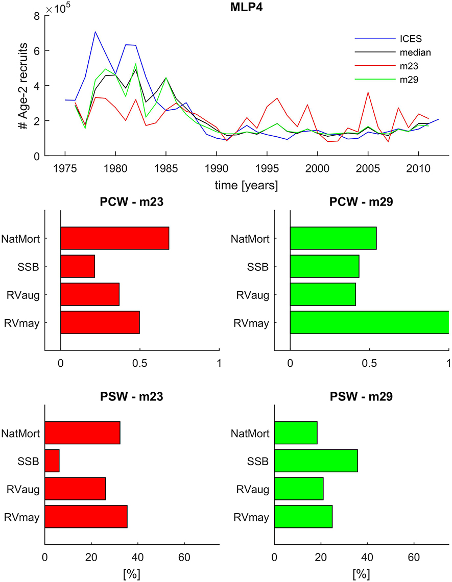
Figure 8. Comparison of the ensemble median and two selected ensemble member model recruitment time series predictions and variable importance estimates from the MLP4 model ensemble. Top panel: time series comparison between the ICES reference values (blue line), the ensemble median (black line), and two selected ensemble member models (m23, red line; and m29, green line) representing extreme ends of the ensemble prediction range. The two Bottom panels show the PCW and PSW variable importance estimates for the m23 ensemble member (left) and the m29 ensemble member (right).
In the four bottom panels of Figure 8 we analyze the differences in assigned connection weights between m23 and m29. In the case of m23, both the PCW and PSW approach lead to a similar conclusion that NatMort and RVmay were most influential in the model with only their rank reversed in the two approaches. SSB played a visibly lower role than all other input variables. In the case of m29, there are very strong differences between PCW- and PSW-based interpretations of the variable importance. While both PCW and PSW point at an increased role of SSB in m29 relative to m23, the latter assigns nearly 40% relative importance to SSB making it the key variable in the model. The PCW approach draws a very different picture with RVmay being by far the most dominant input variable, with NatMort also having a stronger connection weight to the output than SSB.
In order to try and resolve which approach draws a more accurate picture of variable importance in MLP4, we actually use the results of MLP5 which we know was solely based on the relationship between SSB and number of recruits. Figure 7 clearly illustrated that SSB-based MLP5 captured neither the timing nor the magnitude of the very high recruitment events from the beginning of the time series under study. It is therefore highly unlikely that assigning a higher relative weight to SSB would make m29 fit the high recruitment regime so much better than m23. On the other hand, giving more weight to SSB also does not explain the large overestimates in the low recruitment period, as MLP5 rather tended to underestimate recruitment after 1990. Thus, we conclude based on these observations that the PCW approach is more adequate to describing the variable importance in ANN models. It therefore also follows that RVmay might be the key variable needed to correctly project high recruitment events 2 years ahead. On the other hand, we also note that m29 projects false recruitment peaks, i.e., in 1985 and in 1996. Figure 2 reveals that there was a large increase in RVmay in 1994, 2 years prior to the project 1996 peak. It thus appears that a high RVmay in that year did not lead to a marked increase in recruitment, as predicted by m29, and that other factors need also be considered. Therefore, while it appears that NatMort and RVmay are key predictors for FishANN in general, the challenge remains to assign such relative weights to SSB and RVaug to further maximize the 2-year ahead predictive capacity of MLP4.
Moreover, we conclude based on these results that it is imperative not to assign a single fixed set of weights to individual processes represented by the selected input variables in Baltic cod recruitment models as their role in explaining recruitment patterns is very likely shifting depending on the environmental and recruitment regime (see also Margonski et al., 2010 for a discussion on that). Due to the adaptive structure of neural networks (i.e., variable activation of its computing units in response to changes in the input space), mimicking a set of weighted regression models in place of a single best fit model, such a variable distribution of weights is accomplished. Nonetheless, as indicated by the substantial differences between individual model ensemble members, distinct patterns of assigned weights may lead to model projections that are both statistically sound (high performance in terms of r2 and MSE) but which have distinct biases of great consequence in potentially using these tools as support for fish stock management.
One approach would be to use expert judgment or another criterion (e.g., precautionary) to select a single best algorithm. The second approach, preferred by us, is to take an ensemble median/mean result with associated confidence intervals from a number of algorithms of the same structure, both in terms of complexity of the computing units and the number of input variables considered. In this study we also demonstrated that taking the ensemble approach still enables interpretation of variable importance through a sum of both positive and negative non-linear interactions inside an ANN model. We thus presented a pragmatic approach to a very complex problem of predicting fish recruitment under a highly variable environment.
As a potential future development, we hypothesize that applying a weighted majority vote scheme to our ensemble model building in place of the simple median majority vote would further increase the probability of correctly classifying recruitment numbers under unknown sets of inputs variables (Kuncheva, 2004). Implementing such a more complex ensemble scheme is currently hindered by the limited number of sample points in the training dataset, but is likely necessary when dealing with very contrasting environmental and recruitment regimes as in case of the eastern Baltic cod.
Assumptions and Limitations
At this stage, there are some points we need to put into consideration. First, more data may be needed to ensure the actual quality of prediction and training. As stated in Doan and Liong (2004) “the length of the test set has an impact on the prediction capability of the trained model” and our results, given the small amount of data in which the model was trained in, could be open to interpretations. Lek et al. (1996) mention that “repeated resampling of test data sets reduces the potential for sampling error caused by choice of a validation or test data set.” We believe we have used means to address to this issue (i.e., k-fold cross validation) but a longer data set could provide a better overview. While sampling error is not common when “extremely large and functionally homogenous data sets are used and it is likely to be a factor when used for actual ecological data sets where data availability is limited” (Kemp et al., 2007). This could be a reason behind the fact that the model underestimates high recruitment. It is also possible that data may contain some errors. FishANN seems to constantly overestimate one specific recruitment year. At this point, it needs to be said that we didn't account deep-water salinity data in our study, as suggested by Heikinheimo (2008). We would have considered including average deep-water salinity as an additional input variable, should its higher explanatory power relative to RV be also relevant in our case. It is noted that Heikinheimo (2008) examined the variability in Baltic cod age-0 recruitment. All in all, deep-water salinity data was not included due to lack of sufficient availability of the data set. The ICES database offers access to relevant salinity data only until 2004. In order to facilitate reproducibility of results we opted to restrict ourselves to those input variables that are readily available, even though this information could add potential improvement of model predictive skills.
Third, we assumed for our data that mechanisms across Baltic subdivisions are roughly the same, since the integrated abundance of all spawning areas should be unaffected by transport between spawning areas (Köster et al., 2005). We kept this spatial homogeneity within the Central Baltic, similar to studies by Sparholt (1996) and Jarre-Teichmann et al. (2000). We can't be sure to what extent this decision affects the interpretations of complex non-linear relationships for recruitment.
Fourth, the level of analysis in variable importance presented is restricted to semi-linear relations. There might be some additional non-linear effects between them. The question if the available inputs capture this encrypted variability may be more suitable to investigate with emerging tools for non-linear analysis of the relationship of variables used in neural network models (e.g. Fischer, 2015).
The “black box” term is no longer an appropriate term for ANNs. Recent advances in the field of environmental sciences have provided a “set of techniques to determine the relative importance of each input variable” (Fischer, 2015). These techniques include sensitivity analyses (Lek et al., 1996; Recknagel et al., 1997), partial derivatives (Dimopoulos et al., 1999; Reyjol et al., 2001; Gevrey et al., 2006), “input variable relevancies and neural interpretation diagrams” (Ozesmi and Ozesmi, 1999), significance randomization tests (Olden, 2000; Olden and Jackson, 2002). All these approaches are “based on the fact that the contribution of each independent variable depends on the magnitude and direction of the connection weights between neurons” (Olden et al., 2008). However, only a handful of methods have been documented for visualizing non-linear effects of input variables in literature (Garson, 1991; Dimopoulos et al., 1995, 1999; Lek et al., 1996; Fischer, 2015), an important issue to consider when dealing with complex ecosystem scenarios. So far, to our knowledge, there are no relevant studies using these techniques for predicting fish recruitment with ANNs.
Recommendations for Future Work
In 2008, Houde (2008) highlighted some critical research needs in understanding causes of recruitment variability:
• Implementing/continuing long-term surveys on early-life stages.
• Better understanding of larval behavior.
• New and improved coupled biological-physical models: Most coupled biological-physical models have been developed as “explanatory or inferential tools” (Miller, 2007) and relatively few as tools to test hypotheses: the biggest contribution to understanding variability in recruitment ultimately may come from that approach.
• Research that goes beyond life stages.
• Understanding effects of climate change.
• To enable not only short-term but also long-term recruitment projections under scenarios of climate change/variability.
For the future, the statistical nature of ANNs could be combined with dynamic IBMs, fuzzy logic (Chen and Ware, 1999; Chen and Hare, 2006) or expert knowledge to address more complex long term recruitment scenario forecasting in fisheries. By combining process knowledge and statistics (e.g., capelin migration model—Huse and Ellingsen, 2008) we could also enable future scenario testing for long term recruitment hypotheses, and provide “continuous learning” operational predictive models, i.e., with evolving connection weights. This approach, together with an articulate methodology to overview ranking of non-linear variable importance techniques, could enable automated process monitoring, biological systems control, and advance decision making to a new level. We believe that this might be an appropriate approach for a CAS and that ANN tools can contribute significantly toward this direction. The case of the Baltic cod stock exemplifies the multitude of effects biotic interactions (clupeid predation on cod eggs, competition between clupeids, and cod larvae for common zooplankton resources) and climate variability may have on a fish stock, and it underscores the importance of knowledge of these processes for understanding the dynamics of fish stocks.
Author Contributions
All authors listed, have made substantial, direct and intellectual contribution to the work, and approved it for publication.
Conflict of Interest Statement
The authors declare that the research was conducted in the absence of any commercial or financial relationships that could be construed as a potential conflict of interest.
Acknowledgments
The authors of this paper would like to thank M. Plikshs, B. R. Mackenzie, and F.W. Köster for contributing to obtaining important datasets to carry on this study. Funding for MS and AP was provided by the Danish Technical University. DK was partially funded by the Danish Technical University and partially self-funded.
References
Amari, S., Murata, N., Müller, K. R., Finke, M., and Yang, H. (1997). Asymptotic statistical theory of overtraining and cross-validation. IEEE Trans. Neural Netw. 8, 985–996. doi: 10.1109/72.623200
Archontoula, C., Michaela, S., and Nikolas, S. (2003). Comparative assessment of neural networks and regression models for forecasting summertime ozone in Athens. Sci. Total Environ. 313, 1–13. doi: 10.1016/S0048-9697(03)00335-8
Bailey, K. M., Ciannelli, L., Bond, N. A., Belgrano, A., and Stenseth, N. C. (2005). Recruitment of walleye pollock in a physically and biologically complex ecosystem: a new perspective. Prog. Oceanogr. 67, 24–42. doi: 10.1016/j.pocean.2005.06.001
Baran, P., Lek, S., Delacoste, M., and Belaud, A. (1996). Stochastic models that predict trout population density or biomass on a mesohabitat scale. Hydrobiologia 337, 1–9. doi: 10.1007/BF00028502
Beverton, R. J. H., and Holt, S. J. (1957). On the Dynamics of Exploited Fish Populations. Fishery Investigations Series II, Vol. XIX. London: Ministry of Agriculture, Fisheries and Food.
Brey, T., Jarre-Teichmann, A., and Borlich, O. (1997). Artificial neural network versus multiple linear regression: predicting P/B ratios from empirical data. Mar. Ecol. Prog. Ser. 140, 251–256. doi: 10.3354/meps140251
Burden, F. R., and Winkler, D. A. (1999). Robust QSAR models using Bayesian regularized neural networks. J. Med. Chem. 42, 3183–3187. doi: 10.1021/jm980697n
Burden, F. R., and Winkler, D. A. (2000). A quantitative structure-activity relationships model for the acute toxicity of substituted benzenes to tetrahymena pyriformis Using Bayesian-regularized neural networks. Chem. Res. Toxicol. 13, 436–440. doi: 10.1021/tx9900627
Casini, M., Hjelm, J., Molinero, J. C., Lövgren, J., Cardinale, M., Bartolino, V., et al. (2009). Trophic cascades promote threshold-like shifts in pelagic marine ecosystems. Proc. Natl. Acad. Sci. U.S.A. 106, 197–202. doi: 10.1073/pnas.0806649105
Chen, D.-G., and Hare, S. R. (2006). Neural network and fuzzy logic models for pacific halibut recruitment analysis. Ecol. Model. 195, 11–19. doi: 10.1016/j.ecolmodel.2005.11.004
Chen, D. G., Hargreaves, N. B., Ware, D. M., and Liu, Y. (2000). A fuzzy logic model with genetic algorithm for analyzing fish stock-recruitment relationships. Can. J. Fish. Aquat. Sci. 57, 1878–1887. doi: 10.1139/f00-141
Chen, D. G., and Ware, D. M. (1999). A neural network model for forecasting fish stock recruitment. Can. J. Fish. Aquat. Sci. 56, 2385–2396. doi: 10.1139/f99-178
Cushing, D. (1971). The dependence of recruitment on parent stock in different groups of fishes. ICES J. Mar. Sci. 33:340. doi: 10.1093/icesjms/33.3.340
Cushing, D. H. (1996). “Towards a science of recruitment in fish populations,” in Excellence in Ecology. Oldendorf/Luhe: Ecology Institute.
De Oliveira, J. A., Uriarte, A., and Roel, B. (2005). Potential improvements in the management of Bay of Biscay anchovy by incorporating environmental indices as recruitment predictors. Fish. Res. 75, 2–14. doi: 10.1016/j.fishres.2005.05.005
De Oña, J., and Garrido, C. (2014). Extracting the contribution of independent variables in neural network models: a new approach to handle instability. Neural Comput. Appl. 25, 859–869. doi: 10.1007/s00521-014-1573-5
Dimopoulos, I., Chronopoulos, J., Chronopoulou-Sereli, A., and Lek, S. (1999). Neural network models to study relationships between lead concentration in grasses and permanent urban descriptors in Athens city (Greece). Ecol. Model. 120, 157–165. doi: 10.1016/S0304-3800(99)00099-X
Dimopoulos, Y., Bourret, P., and Lek, S. (1995). Use of some sensitivity criteria for choosing networks with good generalization. Neural Process Lett. 2, 1–4. doi: 10.1007/BF02309007
Doak, D. F., Estes, J. A., Halpern, B. S., Jacob, U., Lindberg, D. R., Lovvorn, J., et al. (2008). Understanding and predicting ecological dynamics: are major surprises inevitable. Ecology 89, 952–961. doi: 10.1890/07-0965.1
Doan, C. D., and Liong, S. Y. (2004). “Generalization for multilayer neural network bayesian regularization or early stopping,” in Proceedings of the 2nd Conference Asia Pacific Association of Hydrology and Water Resources (Singapore), 5–8.
Dreyfus-León, M., and Chen, D. G. (2007). Recruitment prediction with genetic algorithms with application to the Pacific Herring fishery. Ecol. Model. 203, 141–146. doi: 10.1016/j.ecolmodel.2005.09.016
Dreyfus-León, M., and Schweigert, J. (2008). Recruitment prediction for Pacific herring (Clupea pallasi) on the west coast of Vancouver Island, Canada. Ecol. Inform. 3, 202–206. doi: 10.1016/j.ecoinf.2008.02.003
Eero, M., Hjelm, J., Behrens, J., Buchmann, K., Cardinale, M., Casini, M., et al. (2015). Eastern Baltic cod in distress: biological changes and challenges for stock assessment. ICES J. Mar. Sci. 72, 2180–2186. doi: 10.1093/icesjms/fsv109
Eero, M., Köster, F. W., and Vinther, M. (2012). Why is the Eastern Baltic cod recovering? Mar. Policy 36, 235–240. doi: 10.1016/j.marpol.2011.05.010
Fang, W. T., Chu, H. J., and Cheng, B. Y. (2009). Modeling waterbird diversity in irrigation ponds of Taoyuan, Taiwan using an artificial neural network approach. Paddy Water Environ. 7, 209–216. doi: 10.1007/s10333-009-0164-z
Fernandes, J. A., Irigoien, X., Goikoetxea, N., Lozano, J. A., Inza, I., Pérez, A., et al. (2010). Fish recruitment prediction, using robust supervised classification methods'. Ecol. Model. 221, 338–352. doi: 10.1016/j.ecolmodel.2009.09.020
Fernandes, J. A., Irigoien, X., Lozano, J. A., Inza, I., Goikoetxea, N., and Pérez, A. (2015). Evaluating machine-learning techniques for recruitment forecasting of seven North East Atlantic fish species. Ecol. Inform. 25, 35–42. doi: 10.1016/j.ecoinf.2014.11.004
Fernandes, J. A., Lozano, J. A., Inza, I., Irigoien, X., Pérez, A., and Rodríguez, J. D. (2013). Supervised pre-processing approaches in multiple class variables classification for fish recruitment forecasting. Environ. Model. Softw. 40, 245–254. doi: 10.1016/j.envsoft.2012.10.001
Fischer, A. (2015). How to determine the unique contributions of input-variables to the nonlinear regression function of a multilayer perceptron. Ecol. Model. 309, 60–63. doi: 10.1016/j.ecolmodel.2015.04.015
Fuchs, F. (1996). “Modelling of interaction in environment and cod using a neural network,” in ICES, CM 1996/C+J:5 (Copenhagen).
Garson, G. D. (1991). Interpreting neural network connection weights. Artif. Intell. Expert 6, 47–51.
Gevrey, M., Dimopoulos, I., and Lek, S. (2006). Two-way interaction of input variables in the sensitivity analysis of neural network models. Ecol. Model. 195, 43–50. doi: 10.1016/j.ecolmodel.2005.11.008
Gevrey, M., Dimopoulos, L., and Lek, S. (2003). Review and comparison of methods to study the contribution of variables in artificial neural network models. Ecol. Model. 160, 249–264. doi: 10.1016/S0304-3800(02)00257-0
Glaser, S. M., Ye, H., Maunder, M., MacCall, A., Fogarty, M., and Sugihara, G. (2011). Detecting and forecasting complex nonlinear dynamics in spatially structured catch-per-unit-effort time series for North Pacific albacore (Thunnus alalunga). Can. J. Fish. Aquat. Sci. 68, 400–412. doi: 10.1139/F10-160
Goh, A. T. C. (1995). Back-propagation neural networks for modelling complex systems. Artif. Intell. Eng. 9, 143–151.
Hastie, T., Tibishrani, R., and Freidman, J. (2001). The Elements of Statistical Learning: Data Mining, Inference and Prediction. New York, NY: Springer
Heikinheimo, O. (2008). Average salinity as an index for environmental forcing on cod recruitment in the Baltic Sea. Boreal Environ. Res. 13, 457–464.
Hornik, K., and White, H. (1989). Multilayer feedforward networks are universal approximators. Neural Netw. 2, 359–366. doi: 10.1016/0893-6080(89)90020-8
Houde, E. D. (2008). Emerging from Hjorts shadow. J. Northwest Atl. Fish. Sci. 41, 53–70. doi: 10.2960/J.v41.m634
Huse, G., and Ellingsen, I. (2008). Capelin migrations and climate change–a modelling analysis. Clim. Change 87, 177–197. doi: 10.1007/s10584-007-9347-z
Ibarra, A. A., Gevrey, M., Park, Y. S., Lim, P., and Lek, S. (2003). Modelling the factors that influence fish guilds composition using a back-propagation network: assessment of metrics for indices of biotic integrity. Ecol. Model. 160, 281–290. doi: 10.1016/S0304-3800(02)00259-4
ICES, R. (2010). Report of the Baltic Fisheries Assessment Working Group (WGBFAS). ICES Headquarters, Copenhagen, 633.
Jarre-Teichmann, A., Wieland, K., MacKenzie, B., Hinrichsen, H. H., Plikshs, M., and Aro, E. (2000). Stock recruitment relationships for cod (Gadus morhua L.) in the central Baltic Sea incorporating environmental variability. Arch. Fish. Mar. Res. 48, 97–123.
Joy, M. K., and Death, R. G. (2004). Predictive modelling and spatial mapping of freshwater fish and decapod assemblages using GIS and neural networks. Freshwater Biol. 49, 1036–1052. doi: 10.1111/j.1365-2427.2004.01248.x
Kasabov, N. K. (1996). Foundations of Neural Networks, Fuzzy Systems, and Knowledge Engineering. Cambridge, MA: MIT Press.
Kemp, S. J., Zaradic, P., and Hansen, F. (2007). An approach for determining relative input parameter importance and significance in artificial neural networks. Ecol. Model. 204, 326–334. doi: 10.1016/j.ecolmodel.2007.01.009
Kimes, D. S., Nelson, R. F., and Fifer, S. T. (2000). “Predicting ecologically important vegetation variables from remotely sensed optical/ radar data using neural networks,” in Artificial Neuronal Networks: Application to Ecology and Evolution, eds S. Lek and J. F. Guegan (Berlin; Heidelberg: Springer-Verlag), 31–44.
Komatsu, T., Aoki, I., Mitani, I., and Ishii, T. (1994). Prediction of the catch of Japanese sardine larvae in Sagami Bay using a neural network. Fish. Sci. 60, 385–391.
Köster, F. W., Hinrichsen, H. H., St. John, M. A., Schnack, D., MacKenzie, B. R., Tomkiewicz, J., et al. (2001). Developing Baltic cod recruitment models. II. Incorporation of environmental variability and species interaction. Can. J. Fish. Aquat. Sci. 58, 1534–1556. doi: 10.1139/f01-093
Köster, F. W., Hinrichsen, H.-H., Schnack, D., St. John, M. A., Mackenzie, B. R., Tomkiewicz, J., et al. (2003). Recruitment of Baltic cod and sprat stocks: identification of critical life stages and incorporation of environmental variability into stock–recruitment relationships. Sci. Mar. 67, 129–154. doi: 10.3989/scimar.2003.67s1129
Köster, F. W., and Möllmann, C. (2000). Trophodynamic control by clupeid predators on recruitment success in Baltic cod? ICES J. Mar. Sci. 57, 310–323. doi: 10.1006/jmsc.1999.0528
Köster, F. W., Möllmann, C., Hinrichsen, H. H., Wieland, K., Tomkiewicz, J., Kraus, G., et al. (2005). Baltic cod recruitment–the impact of climate variability on key processes. ICES J. Mar. Sci. 62, 1408–1425. doi: 10.1016/j.icesjms.2005.05.004
Kuncheva, L. I. (2004). Combining Pattern Classifiers: Methods and Algorithms. Hoboken, NJ: John Wiley & Sons.
Laë, R., Lek, S., and Moreau, J. (1999). Predicting fish yield of African lakes using neural networks. Ecol. Model. 120, 325–335.
Lawrence, J. (1993). Introduction to Neural Networks: Design, Theory, and Application. Nevada, CA: California Scientific Software Press.
Lek, S., Belaud, A., Dimopoulos, I., Lauga, J., and Moreau, J. (1995). Improved estimation, using neural networks, of the food consumption of fish populations. Mar. Freshwater Res. 46, 1229–1236.
Lek, S., Delacoste, M., Baran, P., Dimopoulos, I., Lauga, J., and Aulagnier, S. (1996). Application of neural networks to modeling nonlinear relationships in ecology. Ecol. Model. 90, 39–52. doi: 10.1016/0304-3800(95)00142-5
Lek, S., and Guegan, J. F. (2000). Artificial Neural Networks: Application to Ecology and Evolution. New York, NY: Springer.
Lek, S., Scardi, M., Verdonschot, P. F. M., Descy, J. P., and Park, Y. S. (2005). Modelling Community Structure in Freshwater Ecosystems. New York, NY: Springer.
Levin, S. A. (2005). Self-organization and the emergence of complexity in ecological systems. Bioscience 55, 1075–1079. doi: 10.1641/0006-3568(2005)055[1075:SATEOC]2.0.CO;2
Levin, S. A., and Lubchenco, J. (2008). Resilience, robustness, and marine ecosystem-based management. Bioscience 58, 27–32. doi: 10.1641/B580107
Lewy, P., and Vinther, M. (2004). A Stochastic Age-Length-Structured Multispecies Model Applied to North Sea Stocks. Vigo: ICES CM.
Lindegren, M., Möllmann, C., Nielsen, A., Brander, K., MacKenzie, B. R., and Stenseth, N. C. (2010). Ecological forecasting under climate change: the case of Baltic cod. Proc. Biol. Sci. 277, 2121–2130. doi: 10.1098/rspb.2010.0353
MacKenzie, B. R., Horbowy, J., and Koster, F. W. (2008). Incorporating environmental variability in stock assessment: predicting recruitment, spawner biomass, and landings of sprat (Sprattus sprattus) in the Baltic Sea. Can. J. Fish. Aquat. Sci. 65, 1334–1341. doi: 10.1139/F08-051
MacKenzie, B. R., Meier, H. M., Lindegren, M., Neuenfeldt, S., Eero, M., Blenckner, T., et al. (2012). Impact of climate change on fish population dynamics in the Baltic Sea: A dynamical downscaling investigation. Ambio 41, 626–636. doi: 10.1007/s13280-012-0325-y
Mäntyniemi, S. H., Whitlock, R. E., Perälä, T. A., Blomstedt, P. A., Vanhatalo, J. P., Rincón, M. M., et al. (2015). General state-space population dynamics model for Bayesian stock assessment. ICES J. Mar. Sci. J. du Cons. 72, 2209–2222. doi: 10.1093/icesjms/fsv117
Maravelias, C. D., Haralabous, J., and Papaconstantinou, C. (2003). Predicting demersal fish species distributions in the Mediterranean Sea using artificial neural networks. Mar. Ecol. Prog. Ser. 255, 249–258. doi: 10.3354/meps255249
Margonski, P., Hansson, S., Tomczak, M. T., and Grzebielec, R. (2010). Climate influence on Baltic cod, sprat, and herring stock–recruitment relationships. Prog. Oceanogr. 87, 277–288. doi: 10.1016/j.pocean.2010.08.003
Mastrorillo, S., Lek, S., Dauba, F., and Belaud, A. (1997). The use of artificial neural networks to predict the presence of small-bodied fish in a river. Freshwater Biol. 38, 237–246.
Miller, T. J. (2007). Contribution of individual-based coupled physical biological models to understanding recruitment in marine fish populations. Mar. Ecol. Prog. Ser. 347, 127–138. doi: 10.3354/meps06973
Möllmann, C., Blenckner, T., Casini, M., Gårdmark, A., and Lindegren, M. (2011). Beauty is in the eye of the beholder: management of Baltic cod stock requires an ecosystem approach. Mar. Ecol. Prog. Ser. 431, 293–297. doi: 10.3354/meps09205
Möllmann, C., Diekmann, R., Müller-Karulis, B., Kornilovs, G., Plikshs, M., and Axe, P. (2009). Reorganization of a large marine ecosystem due to atmospheric and anthropogenic pressure: a discontinuous regime shift in the Central Baltic Sea. Glob. Change Biol. 15, 1377–1393. doi: 10.1111/j.1365-2486.2008.01814.x
Möllmann, C., Müller-Karulis, B., Kornilovs, G., and St. John, M. A. (2008). Effects of climate and overfishing on zooplankton dynamics and ecosystem structure: regime shifts, trophic cascade, and feedback loops in a simple ecosystem. ICES J. Mar. Sci. 65, 302–310. doi: 10.1093/icesjms/fsm197
Myers, R. A., Bridson, J., and Borrowman, N. J. (1995). “Summary of worldwide spawner and recruitment data,” in Canadian Technical Report of Fisheries and Aquatic Sciences. Ottawa, ON: Government of Canada Publications.
O'Brien, C. M., and Little, A. S. (2006). Incorporation of Process Information into Stock–Recruitment Models. International Council for the Exploration of the Sea (ICES), Cooperative Research Report 282, 1–160.
Olden, J. D. (2000). An artificial neural network approach for studying phytoplankton succession. Hydrobiologia 436, 131–143. doi: 10.1023/A:1026575418649
Olden, J. D., and Jackson, D. A. (2001). Fish habitat relationships in lakes: gaining predictive an explanatory insight by using artificial neural networks. Trans. Am. Fish. Soc. 130, 878–897. doi: 10.1577/1548-8659(2001)130<0878:FHRILG>2.0.CO;2
Olden, J. D., and Jackson, D. A. (2002). Illuminating the black box: a randomization approach for understanding variable contributions in artificial neural networks. Ecol. Model. 154, 135–150. doi: 10.1016/S0304-3800(02)00064-9
Olden, J. D., Joy, M. K., and Death, R. G. (2004). An accurate comparison of methods for quantifying variable importance in artificial neural networks using simulated data. Ecol. Model. 178, 389–397. doi: 10.1016/j.ecolmodel.2004.03.013
Olden, J. D., Lawler, J. J., and Poff, N. L. (2008). Machine learning methods without tears: a primer for ecologists. Q. Rev. Biol. 83, 171–193. doi: 10.1086/587826
Olden, J. D., Vander Zanden, M. J., and Johnson, P. T. (2011). Assessing ecosystem vulnerability to invasive rusty crayfish (Orconectes rusticus). Ecol. Appl. 21, 2587–2599. doi: 10.1890/10-2051.1
Ozesmi, S. L., and Ozesmi, U. (1999). An artificial neural network approach to spatial habitat modelling with interspecific interaction. Ecol. Model. 116, 15–31.
Planque, B., and Buffaz, L. (2008). Quantile regression models for fish recruitment- environment relationships: four case studies. Mar. Ecol. Progr. Ser. 357, 213–223. doi: 10.3354/meps07274
Planque, B., Lindstrøm, U., and Subbey, S. (2014). Non-deterministic modelling of food-web dynamics. PLoS ONE 9:e108243. doi: 10.1371/journal.pone.0108243
Plikshs, M. (2014). Impact of Environmental Variability on Year Class Strength of Baltic Cod (Gadus morhua callarias L.). Doctoral dissertation, Doctoral thesis, Riga: University of Latvia.
Power, A. M., Balbuena, J. A., and Raga, J. A. (2005). Parasite infracommunities as predictors of harvest location of bogue (Boops boops L.): a pilot study using statistical classifiers. Fish. Res. 72, 229–239. doi: 10.1016/j.fishres.2004.10.001
Quetglas, A., Ordines, F., and Guijarro, B. (2011). “The use of Artificial Neural Networks (ANNs) in aquatic ecology,” in Artificial Neural Networks – Application, ed Chi Leung Patrick Hui (Rijeka: Intech Publications), 567–586.
Recknagel, F. (2006). Ecological Informatics: Scope, Techniques and Applications. New York, NY: Springer.
Recknagel, F., French, M., Harkonen, P., and Yabunaka, K. (1997). Artificial neural network approach for modelling and prediction of algal blooms. Ecol. Model. 96, 11–28.
Reyjol, Y., Lim, P., Belaud, A., and Lek, S. (2001). Modelling of microhabitat used by fish in natural and regulated flows in the river Garonne (France). Ecol. Model. 146, 131–142. doi: 10.1016/S0304-3800(01)00301-5
Ricker, W. E. (1954). Stock and recruitment. J. Fish. Res. Board Can. 11, 559–623. doi: 10.1139/f54-039
Röckmann, C., John, M. A. S., Schneider, U. A., and Tol, R. S. (2007). Testing the implications of a permanent or seasonal marine reserve on the population dynamics of Eastern Baltic cod under varying environmental conditions. Fish. Res. 85, 1–13. doi: 10.1016/j.fishres.2006.11.035
Rothschild, B. (2000). Fish stocks and recruitment: the past thirty years. ICES J. Mar. Sci. 57, 191. doi: 10.1006/jmsc.2000.0645
Ruiz, J., Gonzalez-Quiros, R., Prieto, L., and Navarro, G. (2009). A Bayesian model for anchovy (Engraulis encrasicolus): the combined forcing of man and environment. Fish. Oceanogr. 18, 62–76. doi: 10.1111/j.1365-2419.2008.00497.x
Rumelhart, D. E., Hinton, G. E., and Williams, R. J. (1986). Learning representations by back-propagating errors. Nature 323, 533–536. doi: 10.1038/323533a0
Russo, T., Parisi, A., Garofalo, G., Gristina, M., Cataudella, S., and Fiorentino, F. (2014). SMART: a spatially explicit bio-economic model for assessing and managing demersal fisheries, with an application to Italian trawlers in the strait of sicily. PLoS ONE 9:e86222. doi: 10.1371/journal.pone.0086222
Russo, T., Parisi, A., Prorgi, M., Boccoli, F., Cignini, I., Tordoni, M., et al. (2011). When behaviour reveals activity: assigning fishing effort to métiers based on VMS data using artificial neural networks. Fish. Res. 111, 53–64. doi: 10.1016/j.fishres.2011.06.011
Scheffer, M. (2009). Critical Transitions in Nature and Society. Princeton, NJ: Princeton University Press.
Schirripa, M. J., and Colbert, J. J. (2006). Interannual changes in sablefish (Anoplopoma fimbia) recruitment in relation to oceanographic conditions within the California current system. Fish. Oceanogr. 15, 25–36. doi: 10.1111/j.1365-2419.2005.00352.x
Sjöberg, J. (1995). Non-Linear System Identification with Neural Networks. Ph.D. thesis, Department of Electrical Engineering, Linköping University, Sweden.
Sovan, L., Marc, D., Philippe, B., Ioannis, D., Jacques, L., and Stephane, A. (1996). Application of neural networks to modelling nonlinear relationships in ecology. Ecol. Model. 90, 39–52. doi: 10.1016/0304-3800(95)00142-5
Sparholt, H. (1996). Causal correlation between recruitment and spawning stock size of central Baltic cod? ICES J. Mar. Sci. 53:771e779.
Sun, L., Xiao, H., Li, S., and Yang, D. (2009). Forecasting fish stock recruitment and planning optimal harvesting strategies by using neural network. J. Comput. 4, 1075–1082. doi: 10.4304/jcp.4.11.1075-1082
Suryanarayana, I., Braibanti, A., Rao, R. S., Ramam, V. A., Sudarsan, D., and Rao, G. N. (2008). Neural networks in fisheries research. Fish. Res. 92, 115–139. doi: 10.1016/j.fishres.2008.01.012
Uusitalo, L. (2007). Advantages and challenges of Bayesian networks in environmental modelling. Ecol. Model. 203, 312–318. doi: 10.1016/j.ecolmodel.2006.11.033
Wagner, R., Obach, M., Werner, H., and Schmidt, H.-H. (2006). Artificial neural nets and abundance prediction of aquatic insects in small streams. Ecol. Inform. 1, 423–430. doi: 10.1016/j.ecoinf.2006.07.002
Watts, M. J., and Worner, S. P. (2008). Using artificial neural networks to determine the relative contribution of abiotic factors influencing the establishment of insect pest species. Ecol. Inform. 3, 64–74. doi: 10.1016/j.ecoinf.2007.06.004
Wieland, K., and Jarre-Teichmann, A. (1997). Prediction of vertical distribution and ambient development temperature of Baltic cod, Gadus morhua L., eggs. Fish. Oceanogr. 6, 172–187. doi: 10.1046/j.1365-2419.1997.00038.x
Yuan, H., Gu, Y., Wang, J., Chen, Y., and Chen, X. (2012). “Study on the medium and long term of fishery forecasting based on neural network,” in Artificial Intelligence and Computational Intelligence, eds J. Lei, F. L. Wang, H. Deng, and D. Miao (Berlin; Heidelberg: Springer), 626–633.
Keywords: baltic cod, recruitment, artificial neural networks
Citation: Krekoukiotis D, Palacz AP and St. John MA (2016) Assessing the Role of Environmental Factors on Baltic Cod Recruitment, a Complex Adaptive System Emergent Property. Front. Mar. Sci. 3:126. doi: 10.3389/fmars.2016.00126
Received: 29 February 2016; Accepted: 06 July 2016;
Published: 25 July 2016.
Edited by:
Cosimo Solidoro, Ogs (Istituto Nazionale di Oceanografia e di Geofisica Sperimentale), ItalyReviewed by:
George Triantafyllou, Hellenic Centre for Marine Research, GreeceTommaso Russo, University of Rome Tor Vergata, Italy
Copyright © 2016 Krekoukiotis, Palacz and St. John. This is an open-access article distributed under the terms of the Creative Commons Attribution License (CC BY). The use, distribution or reproduction in other forums is permitted, provided the original author(s) or licensor are credited and that the original publication in this journal is cited, in accordance with accepted academic practice. No use, distribution or reproduction is permitted which does not comply with these terms.
*Correspondence: Dionysis Krekoukiotis, dikr@aqua.dtu.dk
†Present Address: Artur Piotr Palacz, International Ocean Carbon Coordination Project, Institute of Oceanology of the Polish Academy of Sciences, Sopot, Poland