Assessing Drivers of Coastal Primary Production in Northern Marguerite Bay, Antarctica

Introduction

The Western Antarctic Peninsula (WAP) is a region where changes in climate have been most pronounced over recent decades, with strong variability superposed on a long-term warming trend (Vaughan et al., 2003; Meredith and King, 2005; Turner et al., 2005, 2016). These changes include shifting patterns in wind direction and speed, a strong reduction sea ice extent and marked glacial retreat (Marshall et al., 2006; Montes-Hugo et al., 2008; Stammerjohn et al., 2008; Rignot et al., 2013; Turner et al., 2013; Stammerjohn and Maksym, 2017). As a result, the physical characteristics of adjacent marine waters are changing. Increasing wind speeds and the diminution of sea ice have resulted in deepening of mixed layers along the northern WAP region (Montes-Hugo et al., 2009). Moreover, the decrease in sea ice extent removes an important source of freshwater which would otherwise enhance salinity stratification of the water column upon melting in spring. In contrast, an increase in glacial melting is observed, due to enhanced upwelling of relatively warm Circumpolar Deep Water (Cook et al., 2016). These changes may have significant consequences for irradiance and nutrient availability. On the one hand, the increase in glacial meltwater promotes stratification and consequently improves light availability. On the other, more frequent and/or deeper mixing could increase the availability of macro- and micro-nutrients, whereas glacial meltwater is generally poor in macronutrients but potentially rich in trace metals such as iron (Gerringa et al., 2012). This interplay between climate change related impacts is likely to have an effect on both the composition and productivity of the phytoplankton community.

The classical Antarctic food web revolves around highly productive sea ice edge blooms consisting of diatoms, where krill can feed and transfer energy up the food chain (reviewed in Ducklow et al., 2012a). These blooms are instigated by the melting of sea ice and increase in light availability after the polar winter. With the appearance of deeper mixed layers, the phytoplankton community has reoriented itself toward higher proportions of smaller flagellates such as haptophytes (generally Phaeocystis) and cryptophytes (Arrigo et al., 1999; Montes-Hugo et al., 2009; Kozlowski et al., 2011; Trimborn et al., 2015; Rozema et al., 2017a). In the WAP region, this shift in phytoplankton community seems further fueled by the replacement of sea ice melt by glacial melt as the major source of freshwater (Moline et al., 2004; Mendes et al., 2013). While diatoms are still the major contributor to phytoplankton biomass, cryptophytes, and haptophytes are increasing in the coastal WAP region (Saba et al., 2014; Rozema et al., 2017a). Our current understanding suggests an association of haptophytes with more unstable water columns, while cryptophytes show increased abundances when these water columns are restabilizing due to glacial meltwater injection.

The occurring shift in the phytoplankton community seems to coincide with changes in the primary productivity (PP) of the coastal WAP ecosystem. Physical properties of the water column, for example stability, influence PP directly and indirectly. A less stable water column means less available light for photosynthesis, but also promotes growth of different phytoplankton groups. Phytoplankton biomass accumulation is limited in years following winters with a more unstable water column due to low sea ice cover during winter (Venables et al., 2013). This potential effect is further strengthened due to the changing species composition as productivity per biomass unit of small flagellates is different to that of diatoms (reviewed in Petrou et al., 2016). For example, Phaeocystis antarctica is thought to be more productive per chlorophyll a (Chl-a) and per captured photon than Fragilariopsis cylindrus, a small diatom associated with the sea ice edge (Arrigo et al., 2010; Alderkamp et al., 2012a). In contrast, data suggest a decreased potential for productivity in cryptophytes than in haptophytes or diatoms due to a smaller photosynthetic cross section (Claustre et al., 1997). A study examining cultured Arctic representatives of these three groups suggest a dependency on temperature; haptophytes only grew faster under higher temperatures (Van de Poll, unpublished data).

Few field-based studies have assessed the relationship between phytoplankton community composition and PP in the Southern Ocean (Uitz et al., 2009; Takao et al., 2012) or the WAP (Claustre et al., 1997; Vernet et al., 2008; Huang et al., 2012). All these studies observed a significant effect of species composition on water column PP. The most extensive study in the coastal WAP observed a positive relation between diatom abundance and water column PP (Vernet et al., 2008). In contrast, a negative relation was observed between cryptophytes and water column PP. Vernet et al. (2008) further estimated that phytoplankton species composition explained 11% of the variability in primary production. Yet relative phytoplankton species abundances are currently not used when modeling PP at the WAP. Estimates of daily depth-integrated PP over 1995–2006 along the WAP ranged from 250 to 1,100 mg C m⁻² d⁻¹. The coastal regions and Marguerite Bay were most productive, reaching maxima of ~5,000–7,200 mg C m⁻² d⁻¹in highly productive years (Ducklow et al., 2012b; Weston et al., 2013; Stukel et al., 2015). A study modeling weekly PP measurements used a simple, but often used, model which fits their data reasonably and leaving room for improvement (Behrenfeld and Falkowski, 1997; Vernet et al., 2012). This model did not take the composition of the phytoplankton or macro nutrient availability into account, parameters previously known to be affected by the observed changes in climate. Investigating these relations will help tuning current global biogeochemistry models, which already incorporated a crude mechanism to describe phytoplankton community composition (e.g., Aumont et al., 2015).

This study aims to understand and model PP in a climatically variable, coastal region of the WAP where large changes in phytoplankton species composition and meltwater dynamics occur. Our main objective is to reassess the relations between PP, phytoplankton biomass, and species composition, light, macronutrient concentrations, and water column properties. Thereby, we study if parameters not traditionally used to model PP, such as variability in phytoplankton species composition and macro nutrient concentrations, would need to be included given rapid changes currently unfolding in the WAP and improve current models (Behrenfeld and Falkowski, 1997; Vernet et al., 2012). Most previously used models are appropriate for open ocean applications and not necessarily coastal systems. To this end, we used a non-assumptive model (Random Forest, Breiman, 2001) based on in situ measurements to discern the contributions of different biological and environmental parameters governing PP. In addition, we seek a minimalistic but optimized model of PP unbiased by our previous understanding of phytoplankton productivity. This optimized model was then used to estimate PP during one austral summer in a region where PP was studied previously to ensure a good validation of our findings with independent studies. Finally, we seek to compare a statistical approach with a more traditional mechanistic method of estimating PP (Platt et al., 1980; Weston et al., 2013).

The basis for our modeling approaches was formed by field measurements collected at the British Antarctic Survey's Rothera Research Station in northern Marguerite Bay. Here, the year-round Rothera Oceanographic and Biological Time Series (RaTS) program, representing the larger northern Marguerite Bay region, provides the infrastructure and scientific context to understand the dynamics in phytoplankton productivity (Venables and Meredith, 2014). Previous studies have shown a variable, yet generally high, level of phytoplankton biomass dominated by diatoms during summers in this region (Annett et al., 2010; Kozlowski et al., 2011; Rozema et al., 2017a). Phytoplankton biomass, both total and per major taxonomic group, was shown to be related to summer water column stability which, in turn, was driven by winter sea ice cover (Venables et al., 2013; Rozema et al., 2017a). Typically, persistence of summer biomass appears to be regulated by wind mixing events, meltwater input, and nutrient availability (Piquet et al., 2011; Rozema et al., 2017b). The variability at this coastal site, where PP has occasionally been studied, will allow our models to cover a large variability in environmental conditions and phytoplankton community dynamics. Also, the RaTS allows for sufficient context of our estimates on which we can build and validate our non-traditional modeling approach.

Materials and Methods

Site, Sample Collection, and Rats Program

The sampling site was situated in northern Marguerite Bay near Rothera Research Station and is part of the RaTS-program (Figure 1; 67.570°S 68.225°W). Year-round observations of biological and physical processes at this site (15 m depth) started in 1997 (Clarke et al., 2008; Venables et al., 2013; Rozema et al., 2017a). The RaTS site is situated in water ~520 m deep and ~2 km from the nearest shore. Our extensive summer campaign (Nov 2013–Mar 2014) was run in parallel to the RaTS program. CTD and fluorescence measurements to a maximum depth of ~95 m were obtained using a live-feed from the CTD package (SeaBird 19+) equipped with an in-line fluorometer (WS3S, WETLabs), turbidity sensor measuring at 700 nm (ECO NTU, WETLabs), and a spherical sensor (SPQA, LICOR) for Photosynthetically Active Radiation (PAR). Multiple fixed (2, 15, and 75 m) and one variable (depth of fluorescence maximum; F_max) depths were sampled for pigment analysis by HPLC, macronutrients (N, P, and Si) and maximum quantum yield of photosystem II (PSII). Phytoplankton production through ¹⁴Cincorporation was measured at F_max. Surface oxygen isotopes (0 m) used in this study were part of the RaTS program supplemented with a small number (n = 7) of samples collected at 2 m. Desired sampling frequency during summer was twice per week, and once per week for photosynthetic parameters with ¹⁴C incubations (P-E). The fluorescence profiles were calibrated against Chl-a measured by HPLC and collected at 15 m and F_max. All samples were collected by deploying a 12–24 L Niskin bottle with a hand or electric winch on a small boat. After collection, the samples were transported in dark and insulated boxes to the laboratories for further processing. Daily wind speed data from Rothera station was obtained from the British Antarctic Survey (http://www.antarctica.ac.uk/met/metlog/).

FIGURE 1

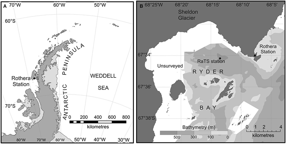
Figure 1. (A): map of the western Antarctic Peninsula, marked with the location of Rothera Research Station on Adelaide Island in northern Marguerite Bay. (B): An expanded view of the immediate vicinity of Rothera, including Ryder Bay where the RaTS long-term monitoring station is situated.

PAR and Light Attenuation

Year-round measurements of PAR were collected every half hour at Rothera station using a fixed sensor (SKP215, Quantum Skye, UK). These measurements were integrated to estimate the daily irradiance dose at the surface (PAR_daily, in μmol photons m⁻² s⁻¹). Attenuation in the water column (K_d in m⁻¹) was derived from linear regression of natural log-transformed, PAR-values as measured with the sensor on the CTD (Kirk, 1983). Estimates of K_d were based on the observations between 5 and 50 m unless PAR was below detection levels at depths shallower than 50 m. The first 5 m were excluded due to frequent shading by the sampling boat. Also, strong deviations in PAR within the water column during a cast, most likely due to changing cloud cover, resulted in a skewed estimate of K_d. Therefore, these casts were split and K_d was calculated by using the curve which had the majority of measurements. These estimates were linearly interpolated to obtain estimates for K_d on days between CTD casts and subsequently used to obtain daily light dose estimates for every depth for every half hour using (Equation 1):

$\begin{array}{cc}\begin{array}{c}E=PA{R}_{daily}\cdot e^{-K_{d}z}\end{array}& \left(1\right)\end{array}$

where E (μmol quanta m⁻² s⁻¹) is the daily irradiance dose at depth z (m) (Kirk, 1983).

Water Column Stability and Stable Oxygen Isotopes

Mixed layer depth (MLD) was defined using the depth at which the Brunt–Väisälä frequency (BVF) was highest, as recommended recently for the WAP (Carvalho et al., 2017). Ocean Data View v4.7.8 was used to calculate the BVF (Schlitzer, 2016). Oxygen isotope samples (δ¹⁸O) were analyzed as described in Meredith et al. (2008). We used the δ¹⁸O and salinity data to derive quantitative estimates of the freshwater contributions from sea ice melt and meteoric water, which is possible since freshwater of meteoric origin is isotopically lighter than that originating from sea ice melt. The two sources of meteoric water are precipitation and glacial meltwater (Craig and Gordon, 1965). Simple budget calculations have shown that glacial discharge is the largest contributor to the meteoric water prevalence in the coastal WAP environment, however this glacial melt may be injected over a broader depth range than direct precipitation, which necessarily impacts the ocean directly at the surface (Meredith et al., 2017).

Macronutrients

Nutrient samples were collected as described earlier (Bown et al., 2017) or as described below. A cross comparison of these two different collection methods during the 2012–2013 season did not yield major differences. Subsamples (2 × 5 mL) for macronutrient analysis were filtered (prefilter: 0.8 μm, membrane: 0.2 μm, Acrodisc Supor PF, Pall, US) and stored in the dark at −20°C (nitrate, nitrite, and phosphate) or 4°C (silicate). Analyses for samples collected using both collection methods were conducted using a Technicon TRAACS 800 Auto-analyzer at the Royal Netherlands Institute for Sea Research, The Netherlands (Bown et al., 2017). Nitrite and nitrate were summed and are presented as N_Tot.

Phytoplankton Pigments

Collection for and measurement of phytoplankton pigments were done using the standard RaTS protocol (Rozema et al., 2017a). In short, phytoplankton cells were collected on GF/F filters (Whatman, US) under low light and at ~2C using a mild vacuum (<0.2 mbar) generated with a water jet pump. After filtration, the filters were snap frozen in liquid nitrogen and stored at −80°C until analysis. For analysis, samples were freeze dried for 48 h prior to extraction in 90% acetone (v/v) at 4°C in the dark for another 48 h. The pigments were separated using a Waters 2,695 HPLC system equipped with a Zorbax Eclipse XDB-C8 column (3.5 μm particle size) as described by van Heukelem and Thomas (2001) and modified by Perl (2009). Pigments were manually identified using retention times and diode array spectroscopy (type 996, Waters, US) before quantification. Calibration of the system was performed using standards (DHI LAB PRODUCTS, Denmark) for chlorophyll c₃, peridinin, 19′-butanoyloxyfucoxanthin, fucoxanthin, neoxanthin, prasinoxanthin, 19′-hexanoyloxyfucoxanthin, alloxanthin, lutein, chlorophyll b, and Chl-a.

CHEMTAX (v1.95) was used to estimate the abundance of various phytoplankton groups (Mackey et al., 1996). This program employs a factor analysis and steepest descent algorithm to find the best fit using initial pigment ratios from previous studies for eight different phytoplankton classes, namely prasinophytes, chlorophytes, dinoflagellates, cryptophytes, two types of haptophytes, and two types of diatoms (Supplementary Table 1, Wright et al., 2009, 2010; Rozema et al., 2017a). Haptophytes were included as two separate groups since Phaeocystis, the most abundant haptophyte in our system, has shown great plasticity in cellular pigment ratios with iron and light availability (as reviewed in van Leeuwe et al., 2014). Also, two diatom groups were included to allow for differentiation in chlorophyll c₃ containing diatoms such as Proboscia spp. and Pseudonitzschia spp. and non-c₃ containing species (unpublished data).

A total of 139 samples were divided over 3 bins. We calculated from city-block distances and clustered the samples according to Ward's method as suggested by Latasa et al. (2010) using Past 2.17c (Hammer et al., 2001). This dendrogram suggested binning of the samples collected at 0–7, 8–49, and 50–75 m bins and the smallest bin size was 40. The initial ratios were as used previously with the RaTS data (Supplementary Table 1; Bown et al., 2017; Rozema et al., 2017a). Neoxanthin and prasinoxanthin were excluded for the 50–75 m bin. Further CHEMTAX settings were as described previously (Kozlowski et al., 2011; Rozema et al., 2017a). CHEMTAX was run 60 times using randomized pigment: Chl-a ratios (±35% of the initial matrix) to obtain the best possible result per bin (Supplementary Table 1; Wright et al., 2009). Both haptophyte and diatom groups as used with CHEMTAX were pooled and renamed to “pooled haptophytes” and “pooled diatoms,” respectively.

Estimating Phytoplankton Biomass

A quenching correction was applied to the upper water column fluorescence, as collected during the CTD casts, to allow for an accurate estimate of the water column biomass. This correction was based on linear regression of Chl-a concentration at 2 and 15 m or F_max (the sample collected at the shallowest depth was used) as estimated from HPLC analysis. If F_max was >>15 m (start summer campaign: late November 2013–Early December 2013) then Chl-a measured at F_max and 2 m were used. The slopes of these regressions were then used to estimate biomass in relation to the calibrated CTD fluorescence for the top layer. We present the corrected phytoplankton biomass estimates as Chl-a_corr. Additionally, standing phytoplankton stocks were calculated by integrating the first 80 m of the water column using Chl-a_corr. The depth of 80 m was chosen as this is generally in the layer of winter water, near the deepest sample for HPLC (75 m) and light does not penetrate this deep during summer (Clarke et al., 2008).

Maximum Quantum Yield of PSII

Triplicate measurements of maximal quantum yield of PSII (F_v/F_m) using a WATER-FT PAM (Walz, Germany) in dark-adapted subsamples (40 mL) allowed for the assessment of the photophysiological state of the phytoplankton community (reviewed in Maxwell and Johnson, 2000). F_v/F_m-values < 0.5 are generally indicative of exposure to stress due to e.g., exposure to excess PAR and/or ultraviolet radiation or nutrient limitation.

Dissolved Inorganic Carbon

Dissolved Inorganic Carbon (DIC) concentrations were used in the calculation of primary production from ¹⁴C measurements. Samples for the analysis of DIC were collected on 8 sampling days (January 15, 25, 30, February 3, 10, 17, 25, and March 3, 2014) in borosilicate glass bottles and analyzed within 20 h of sampling as presented in Jones et al. (2017). DIC concentrations were determined by coulometric analysis according Johnson and Sieburth (1987) and Dickson et al. (2007) using a VINDTA 3C instrument (Versatile INstrument for the Determination of Total Alkalinity, Marianda, Germany). A power function was used to described the relationship between DIC and HPLC derived chlorophyll a concentrations (R² = 0.94, p < 0.001) to estimate DIC concentrations for the calculation of primary production on missing sampling days.

Photosynthesis-Irradiance Measurements

Water collected at the depth of F_max was used to estimate phytoplankton productivity. PP was estimated by constructing P-E curves (n = 16) based on a modified protocol from Lewis and Smith (1983). Seawater subsamples (20 mL) were incubated in a photosynthetron for 4 h under 21 different light intensities (8–713 μmol quanta m⁻² s⁻¹; Osram Powerball HCl-TT 250W in a Jolly symmetrical armature) at in situ (±0.5°C) temperature after the addition of 0.37 MBq ¹⁴C-bicarbonate (PerkinElmer, The Netherlands; >1.7 TBq mmol⁻¹) in clear 60 mL polyethylene terephthalate (PET) bottles (Qorpak, US). After incubation, the samples were filtered onto polycarbonate membrane filters (Millipore, US; 25 mm, 0.4 μm pore size) using a gentile vacuum (<0.1 bar) on a filtration carousel (Millipore, US). After filtration, the filters were acidified with fuming HCl for ~20 min to vent off unincorporated ¹⁴C-bicarbonate. Filters were placed into 20 mL PET scintillation vials (Wheaton, US) and supplemented with 10 mL scintillation cocktail (Ultima Gold, PerkinElmer, The Netherlands). For time zero activity, triplicate samples were prepared, filtered over polycarbonate membrane filters and immediately acidified. For total activity, 10 μL Ethanolamine was added to 100 μL ¹⁴C spiked subsamples in triplicate in 20 mL PET scintillation vials containing a clean polycarbonate membrane filter. Time zero activity and total activity were then treated identically to the other samples. All samples were vortexed and left for 2 days to ensure maximum dispersal of activity throughout the scintillation cocktail before counting activity on a Tri-Carb 2900TR (Packard Instrument Company, US).

The data were converted to DPM after correction for time zero activity (Steeman-Nielsen, 1952), and normalized to Chl-a, as derived from the HPLC analyses, and DIC (see above), and corrected for metabolic discrimination (5%) between ¹²C and ¹⁴C (Ærtebjerg-Nielsen and Bresta, 1984). These data were fitted by least-squares nonlinear regression using the model Equation 2 of Platt et al. (1980), modified by MacIntyre and Cullen (2005):

$\begin{array}{cc}P=P_s\left(1-e^{-\alpha \left(\frac{E}{P_s}\right)}\right)\left(e^{-\beta \left(\frac{E}{P_s}\right)}\right)+P_0& \left(2\right)\end{array}$

where P (μg C μg Chl-a⁻¹ h⁻¹) is the carbon fixation rate at irradiance E, P_s (μg C μg Chl-a⁻¹ h⁻¹) the light-saturated maximum of carbon fixation in the absence of photoinhibition, α [μg C μg Chl-a⁻¹ h⁻¹ (μmol quanta m⁻² s⁻¹)⁻¹] the initial slope of the P-E curve, β [μg C μg Chl-a⁻¹ h⁻¹ (μmol quanta m⁻² s⁻¹)⁻¹] is a measure for photoinhibition, and P₀ (μg C μg Chl-a⁻¹ h⁻¹) is the carbon uptake or release without any irradiance. These parameters were considered characteristic for the phytoplankton throughout the water column at the day of collection.

Constructing and Evaluate Models

Two different methods of calculating phytoplankton carbon uptake were employed. The classical, mechanistic approach relies on the estimations of the P-E parameters, biomass estimates and total irradiance for days without P-E incubations (M_Platt; Platt et al., 1980). These estimates were obtained as discussed below and run through M_platt for every 1 m. Our second statistical approach method uses Random Forest (RF) regressions. RF is a machine learning method which constructs a large number of regression trees by randomly taking subsets of the data and input variables (Breiman, 2001). The major benefits of using such a tool over more traditional (mostly linear) models are: Regression trees allow for (1) non-linear relationships between input and output variables, (2) non-additive interactions between predictor and response variables and (3) correlations between different input variables (Breiman, 2001; Shi and Horvath, 2006). The relevant variables included were phytoplankton biomass, macronutrients, MLD, temperature, salinity, total irradiance and the relative abundance of the three most important phytoplankton groups, namely diatoms, haptophytes and cryptophytes (Behrenfeld and Falkowski, 1997; Arrigo et al., 1999; Dierssen and Smith, 2000; Vernet et al., 2008, 2012; Montes-Hugo et al., 2009; Piquet et al., 2011; Venables et al., 2013; Williams et al., 2016; Bown et al., 2017; Rozema et al., 2017a,b).

For the RF approach, we modeled the log of the PP estimates from the 16 P-E experiments (see above) using the depths for which all the aforementioned variables were available (n = 62). We constructed a model in which all the parameters (M_RFmax) were included and one reduced, optimized model (M_RFmin). During the construction we grew 2,000 trees, and four (M_RFmax) or two (M_RFmin) variables were used at every split. Variables least important in M_RFmax were removed individually until the fit of the new model no longer improved and this became M_RFmin. Partial dependence plots were generated for each variable per model to understand to the relationship with PP. These plots have the input parameter on the horizontal axis and give the range of impact of the input variable on PP. We discussed the importance of each variable to the models above but here we used the shape (and direction) of the curve to understand how this parameter influenced PP in our RF models. Partial dependence plots show the effect of the predictor on the response variable after accounting for the average effects of the other predictors. Therefore, it is the trend, not the actual values, that describes the dependence between both variables.

To assess the predictive power of both RF models, the data were split randomly into a training (80%) and test set (20%). This was repeated 10 times resulting in slightly different models of each type (M_RFmax and M_RFmin). These 10 slightly different models were subsequently tested against the randomly generated test sets using linear regression. We included the mean p and R²-values of these assessments. The “randomForest” package in R (v3.3.1) was used to build our models (Liaw and Wiener, 2002; R Core Team, 2016).

Constructing Input Matrices and Estimating Phytoplankton Productivity

After the construction of the minimal RF model, we aimed to calculate the PP in the water column (0–80 m) over the full course of the season using M_platt and M_RFmin. For this, we needed to obtain full matrices for all parameters used in the models. We used anisotropic ordinary kriging to interpolate both in depth and time using the “gstat” package in R (Pebesma, 2004). First, we optimized the kriging function to best fit the autocorrelation per variable for the depth component using variograms. This function was then used for the interpolation through time. We chose a weighing factor of 0.3 for the time component to allow for the required sensibility needed during short, sudden events such as wind mixing. The matrix for PAR data was constructed as described above. Values for α, β, P₀, and P_s were linearly interpolated from days with P-E incubations. Thus, identical biomass and PAR estimates were used for all modeling approaches.

PP was calculated for every half hour, due to the resolution of the light measurements, and every depth (0–80 m) using M_platt and M_RFmin. The values were summed to obtain daily values. We chose to use a resolution of half an hour as light was highly variable throughout the day and our model included the potential for photoinhibition. Secondly, our RF model included the aforementioned parameters and was run using the constructed matrices. For light in M_RFmin used the summed daily irradiance for all depths. We summed all data for December, January and February as this is traditionally the most productive period and define this as the summer productivity estimates.

Results

Light

PAR availability in the water column was higher during spring (November) than during summer (Figure 2A). Also, PAR in the water column was lowest from December 15th to December 21th. This was related to high turbidity, increasing K_d to >0.30 m⁻¹ as well as low surface irradiance dose (December 23rd and 24th; Figures 2B,C). In contrast, surface irradiance dose peaked at the end of December before gradually decreasing. A brief and sharp increase of PAR at 15 m occurred on January 15thwhen K_d was low. Not until February 14th had PAR penetrated >50 μmol quanta m⁻² s⁻¹ beyond 15 m again and thereafter remained above this level (Figure 2A). The dynamics in K_d strongly coincided with standing phytoplankton biomass. The only major exception was after the short break (December 23rdand 24th) in our sampling effort due to hindrance of drifting sea ice sheets. During these casts, K_d was far higher (>0.30 m⁻¹) than observed at other times in our campaign.

FIGURE 2

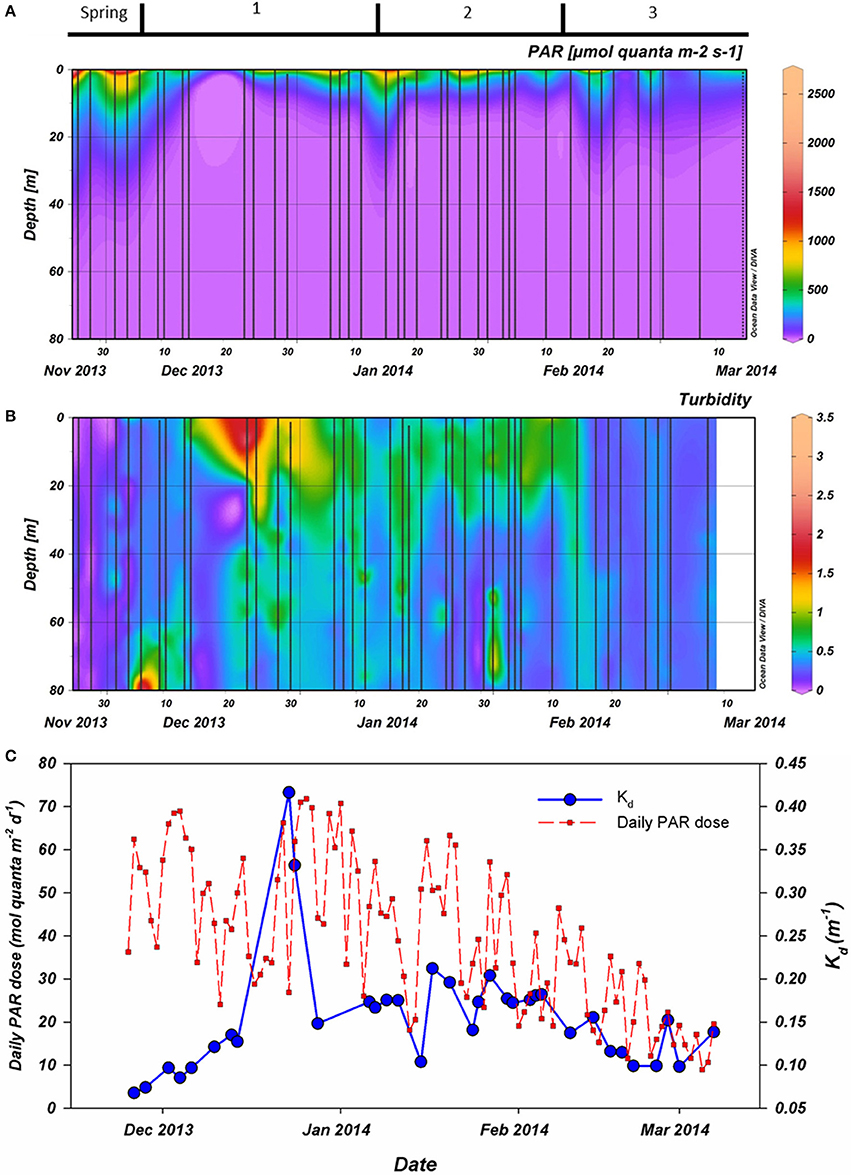
Figure 2. (A): Photosynthetically active radiation (PAR) as measured during CTD casts (vertical casts). (B): Turbidity as also measured during the CTD casts. (C): First, the extinction coefficient (K_d in blue) as calculated using the PAR data collected by CTD. Also, the daily irradiance dose for PAR (red) integrated from continuous measurement at Rothera station. All data were collected during the 2013–2014 season. Period 1 starts on December 6th, period 2 on January 15th and period 3 on February 10th.

Water Column Physics

Our field campaign started (November 26th) during a period where SSTs started to increase slightly while MLD and surface salinity decreased (Spring, Figures 3A,B, 4A). Above zero surface temperatures first occurred on and persisted onwards from December 6th(start of period 1). The MLD during the first half of December was shallow (1 m) while salinity kept decreasing. After a brief period of elevated wind speed and a deepening of the MLD (December 23rd), the water column surface salinity restabilized while the SST increased further (Figures 3A,B, 4A). Maximum SST at 1 m during this summer was 2.7°C on January 6th and 11th. The period of high SSTs was interrupted by an increase of wind speed and deepening of the MLD in mid-January ending period 1 and homogenizing water column temperature and salinity (Figure 4A). This increase in MLD was of a short duration as the water column restabilized within a week. Thereafter, surface temperature increased again with positive temperatures up to a depth of ~30 m and a stable surface salinity (~32.6). These conditions lasted until mid-February when strong winds occurred more frequently, salinity started to increase and SST decreased which resulted in the end of period 2. As in spring, the water column temperature dropped and stayed below 0°C and was more homogenous throughout the water column after February 10th, labeled as period 3.

FIGURE 3

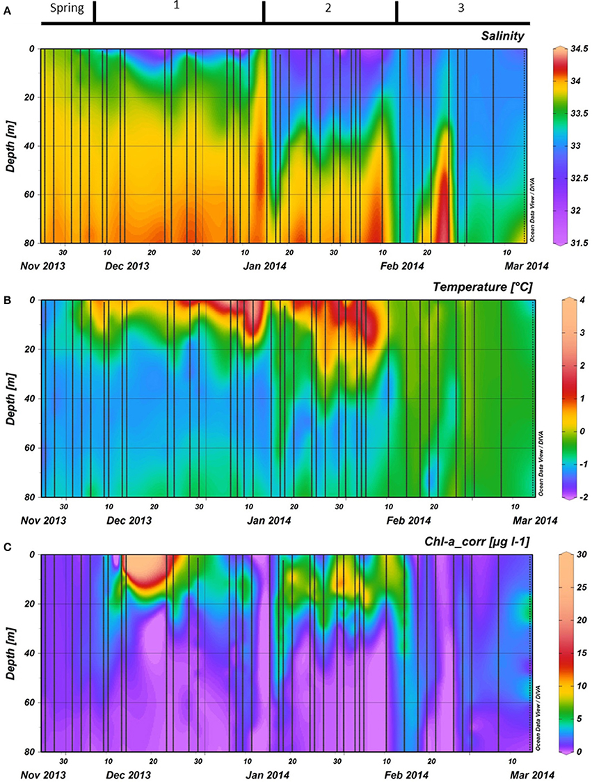
Figure 3. (A): Salinity, (B): Temperature, and (C): Phytoplankton biomass as measured by fluorescence during the vertical CTD casts. Phytoplankton biomass fluorescence was calibrated against chlorophyll a measurements with HPLC and corrected for quenching in top layer using the chlorophyll estimates. All data were collected during the 2013–2014 season at the RaTS site. Period 1 starts on December 6th, period 2 on January 15th and period 3 on February 10th.

FIGURE 4

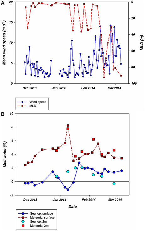
Figure 4. (A): Daily average wind speed (blue) and mixed layer depth (MLD) calculated using the depth of the maximum Brunt–Väisälä frequency. (B): Different fractions of meltwater with different origins. Firstly, samples collected at the surface as part of the RaTS program are divided into the fraction of meteoric origin (dark red) and sea ice origin (dark blue). Additionally, a number of samples collected at the same site, but at 2 m depth also show the two fractions (light red and blue, respectively) and illustrates the effect of very shallow meltwater lenses. All data were collected during the 2013–2014 season. Period 1 starts on December 6th, period 2 on January 15th and period 3 on February 10th.

Freshwater Origin

Sea ice retreat from the preceding winter was late and the contribution of sea ice meltwater to the water column during summer was, although modest at all times, the highest (2.8%) recorded in the RaTS program (Figure 4B; Legge et al., 2017; Meredith et al., 2017). Oxygen isotope data from the surface and at 2 m depth showed an influx of sea ice melt after December 13th, continuing to at least the end of February. The contribution of glacial melt was higher than sea ice melt (mean 4.4%), but also more variable. After an initial increase, freshwater of meteoric origin peaked at 8.3% (also a record for the RaTS program) before dropping to just 3.1% on January 15th as an increase in wind speed mixed the water column (Figure 4A). Both freshwater components increased rapidly after the period of MLD deepening, after which the meteoric freshwater contribution at 2 m depth remained relatively stable at ~4% while the contribution of sea ice melt slowly decreased toward the end of summer.

Macronutrients

Macronutrient concentrations at the end of spring were high with water column averages of 29.0, 1.8, and 83.5 μMfor N_Tot, phosphate, and silicate, respectively (Figure 5). These values were characteristic of the Antarctic winter water, as concentrations at 75 m were only slightly higher. During period 1, the vertical distribution of the macronutrients strongly followed the patterns observed in SSTs. Nutrient concentrations were generally lowest at the surface (2 m). Nutrient concentrations in the first ~15 m strongly decreased over a 10-day period after December 13th. On December 23, all macronutrients were virtually depleted with only 0.01 μM phosphate, 0.06 μM N_Tot, and 0.70 μM silicate left at 2 m depth. This period of depletion lasted until the end of period 1, when nutrients throughout the water column were mixed, restoring 2 m values to the levels similar to those observed before December 13th. Low nutrient concentrations were observed in period 2 with minimum values at 2 m depth on February 5th (13.6 μM silicate, 0.07 μM nitrate and no detectable nitriteor phosphate). This depletion of nutrients persisted to a depth of ~20 m. Period 3 was characterized by a gradual increase in surface nutrient levels.

FIGURE 5

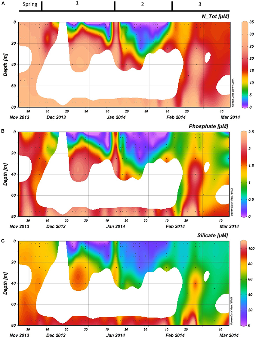
Figure 5. (A): Total nitrogen (nitrate + nitrite), (B): Phosphate, and (C): Silicate concentrations in the water column at the RaTS site. Black dots illustrate the sampling depths. Period 1 starts on December 6th, period 2 on January 15th and period 3 on February 10th.

Phytoplankton Biomass and Species Composition

Phytoplankton biomass accumulated during period 1 (Figure 3C). Relative abundances of diatoms increased at the cost of haptophytes during the start of this period (Figure 6). A sudden increase in phytoplankton biomass (up to 26 μg Chl-a l⁻¹), mainly consisting of small diatoms (Buma et al. unpublished microscopy data; Figure 6, Supplementary Figure 1), coincided with the occurrence of sheets of sea ice in the bay on December 14th. This biomass peak lasted until December 28th after which values dropped to ~5 μg Chl-a l⁻¹. Integrated phytoplankton stocks (0–80 m) followed a similar trend: a large increase between December 10th and 14th, and a steady decrease thereafter (Figure 7). Moreover, F_v/F_m in the top 10 m during the short, yet sharp increase in biomass was lower than expected for the in situ light intensities when compared to the rest of the summer (p < 0.001; Supplementary Figure 2). After the biomass peak, phytoplankton stocks remained stable until the end of period 1. During period 2, diatoms remained the most important taxonomic group although cryptophyte proportions increased (max. 40%) in the surface layer (2 m; Figures 4A, 6). Also, haptophytes increased at 15 m (~15%) until January 30th. Phytoplankton biomass was more evenly distributed over the first 30 m during this period, reaching a maximum concentration of 11 μg Chl-a l⁻¹ and suggested three short periods where biomass increased and decreased (Figure 7). The first was associated with the increase in haptophytes at 15 m, the second and third with diatoms. In period 3, relative abundances of haptophytes and cryptophytes were both elevated in comparison to the previous periods (max. 38 and 47%, respectively) and both phytoplankton groups co-occurred in the first 15 m (Table 2). Diatoms were more abundant at the deep fluorescence maxima. Phytoplankton biomass at 75 m was low and only increased during the two occasions where strong winds caused a deepening of the MLD. Relative group abundance matched those observed in the surface, albeit with a delay of ~30 days (Supplementary Figure 1).

FIGURE 6

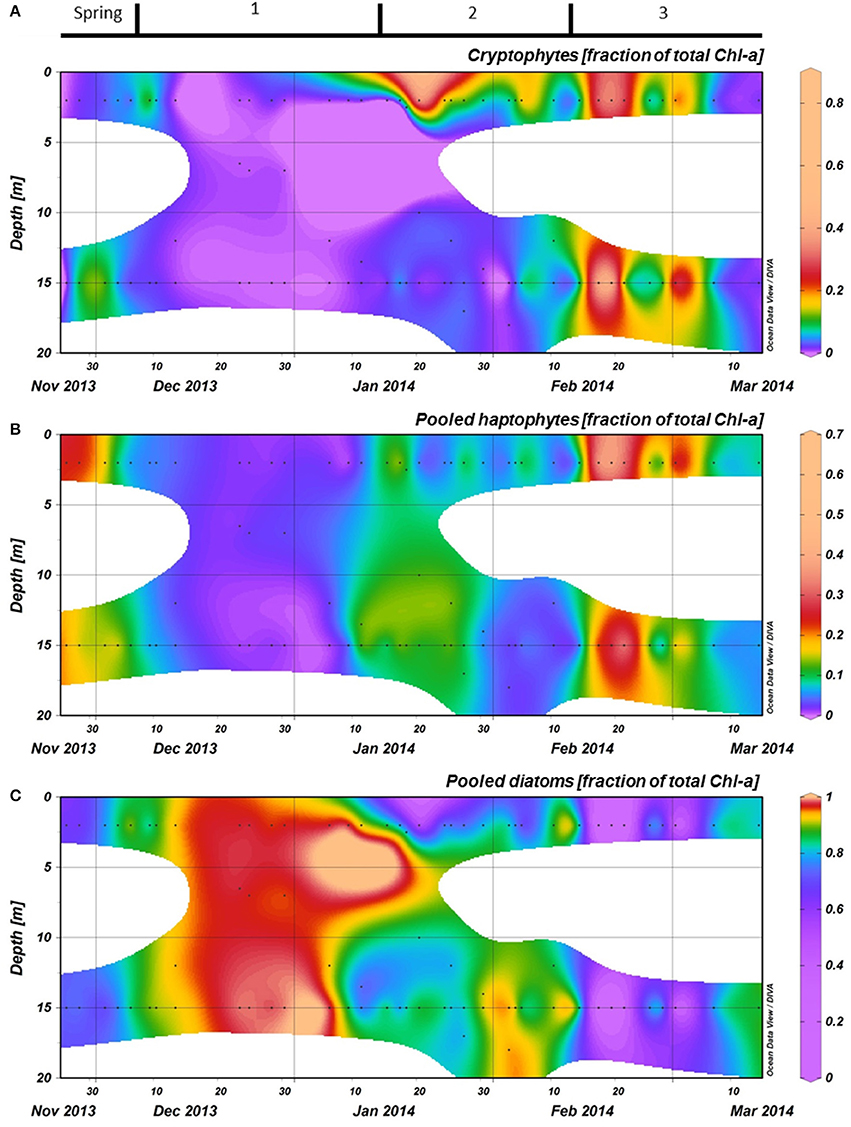
Figure 6. The relative abundances of the three most important phytoplankton groups, as calculated with CHEMTAX using HPLC measurements of pigments, are shown for the top 20 meters at the RaTS site. (A): Pooled diatoms, (B): Pooled haptophytes, and (C): Cryptophytes. Black dots illustrate the sampling depths.

FIGURE 7

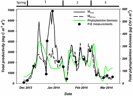
Figure 7. Total, water column integrated primary production as measured during P-E experiments (black dots) or estimated using two modeling approaches. These estimates are based on Platt et al. (1980; solid black line) or the minimal random forest model constructed in this study (dashed black line). Also shown is the water column integrated phytoplankton biomass. All integrations were to a depth of 80 meters. Period 1 starts on December 6th, period 2 on January 15th and period 3 on February 10th.

P-E Measurements

Variability in photosynthetic parameters as obtained from the P-E experiments (n = 16) changed over the course of the summer. At the end of spring (November-early December), α, P_s, and P₀ were low in comparison to the summer values (Table 1). At the end of December, both α and P_s increased >50%. P_s appeared to reach an average of ~4 μg C μg Chl-a⁻¹ h⁻¹for the rest of the summer (January–March) while P₀ increased further to 0.68–0.85 C μg Chl-a⁻¹ h⁻¹. The α also increased further to 0.068–0.083 μg C μg Chl-a⁻¹ h⁻¹ [μmol quanta m⁻² s⁻¹]⁻¹. In contrast, β was very low and only increased to a maximum average of 0.004 μg C μg Chl-a⁻¹ h⁻¹ [μmol quanta m⁻² s⁻¹]⁻¹, suggesting that photoinhibition was of minor importance.

TABLE 1

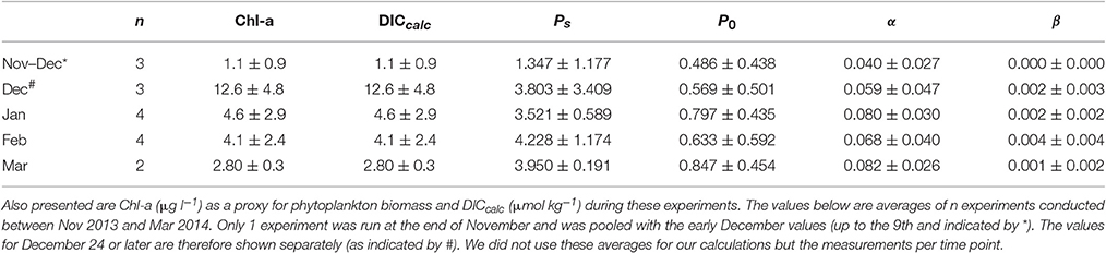
Table 1. Shown below are the mean values (±standard deviation) for photosynthetic parameters P_s and P₀ (both in μg C μg Chl-a⁻¹ h⁻¹), and α and β [both in μg C μg Chl-a⁻¹ h⁻¹(μmol quanta m⁻² s⁻¹)⁻¹] as calculated from the ¹⁴C experiments at F_max.

Using these P-E parameters, we calculated integrated PP for the water column on the days of the experiments (Figure 7). These values ranged from 92.5 (end of November) to 6,907.7 (end of December) mg C m⁻² d⁻¹. While the PP estimates from these experiments showed an increasing trend over the entire month of December, PP on December 23rd was substantially lower. The peak value of 6,907.7 mg C m⁻² d⁻¹occurred on December 30th after which PP decreased reaching a minimum of 438.2 mg C m⁻² d⁻¹on January 15th. PP during period 2 increased again to a maximum of 3,109.5 mg C m⁻² d⁻¹ and lasted until mid-February before stabilizing around 680 mg C m⁻² d⁻¹ during period 3.

Testing Importance of Species Composition

To estimate the potential influence of phytoplankton species composition on PP we compared the log PP at discrete depths where we collected supplementary data (if PP > 0, n = 42) against the relative abundances of the three major phytoplankton groups (Table 2). It appeared that while PP and both diatoms and haptophytes approached a monotonic relation, cryptophytes and PP did not. Linear regressions for these three comparisons yielded r²-values of 0.01, 0.27, and 0.14 (p < 0.001) for cryptophytes, haptophytes and diatoms, respectively. Thus, we opted for spearman rank order analyses, which are less sensitive for non-linear trends (Table 2). We observed a negative relation between PP and haptophytes whereas a larger diatom fraction resulted in higher PP (p < 0.001). However, the relation between cryptophytes and PP was no longer significant (p = 0.36). The opposing trends between haptophytes and diatoms vs. PP were supported by correlations between the phytoplankton groups (Table 2). Haptophytes and cryptophytes were positively related to each other while both were negatively related to diatom abundance (p < 0.001).

TABLE 2

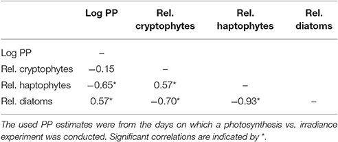
Table 2. Spearman rank order correlations where log PP estimates (n = 42) for the depths for which pigment samples were collected (with PP > 0) were correlated to the calculated relative abundance of the major phytoplankton groups as calculated with CHEMTAX.

Creating RF Models

Using M_RFmax with all the parameters included (p < 0.001, R² = 0.91), we quantified the contribution of the different input parameters on PP using a variable importance plot (Figure 8). Of these parameters, daily PAR was the most important, increasing the mean square error (MSE) by 50.4%. The other two large components were phytoplankton biomass (26.7%) and water temperature (21.6%). The three macronutrients (N_Tot, phosphate and silicate) showed a smaller importance (20.4–17.3%). Salinity (15.5%), MLD (13.6%) and the relative contributions of the major phytoplankton species (7.3–12.2%) influenced the MSE to a lesser extent. The contribution of some of the 12 included parameters was limited, possibly because some of the variability was already explained by a correlated and more important parameter. Therefore, we reduced our first model (M_RFmax) to obtain a more minimalistic model (M_RFmin) with only three parameters that explain 93% of the variability: daily irradiance dose throughout the water column, phytoplankton biomass and N_Tot (Figure 8). The second-best option explained only slightly less of the MSE and included seawater temperature instead of N_Tot. The inclusion of either seawater temperature or N_Tot resulted in highly similar minimal models. A linear correlation analysis on all the samples in which N_Tot was measured (excluding 75 m samples) revealed a strong relation between the two parameters (p < 0.001, r² = 0.67).

FIGURE 8

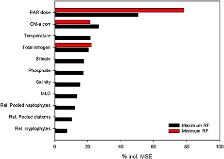
Figure 8. Variable importance plot for the two random forest models build to estimate PP throughout the water column: R_Fmax (black) and R_Fmin (red). The x-axis shows the percentage of reductions in mean square error (MSE) per variable. All variables were included in the maximum model; daily PAR dose in the water column, phytoplankton biomass (chlorophyll a corrected for quenching), temperature, total nitrogen, silicate, phosphate, salinity, mixed layer depth (MLD based on maximum Brunt–Väisälä frequency) and relative abundance of the three most abundant phytoplankton groups. The minimum model excluded variables until a model was reached with the highest possible fit. The importance of the three remaining variables in this model is shown in red.

Partial Response of Variables

After the construction of our models, we analyzed how each of these parameters influenced PP at the depths where all auxiliary data (generally 2, 15, 75 m, and F_max) were available using partial dependence plots (Figure 9). The partial dependence plots for the two different models were highly similar and thus we present M_RFmax as it includes all variables, those for M_RFmin are included in the supporting information (Supplementary Figure 3). Light was the most important factor in both models, the partial dependence plot suggests that when light is not available, PP is strongly decreased. Also, when light is above a certain threshold (~3 mol quanta m⁻² d⁻¹), its effect on PP remains unchanged. Phytoplankton biomass showed a similar trend. PP did not increase further above ~7 μg Chl-a l⁻¹, although the support of this plateau is limited given that it is based on only 10–20% of the data. The three macronutrients had similar trends in relation to PP: the lower the concentration, the higher the PP until it reaches a plateau. Silicate and N_Tot dynamics suggest two distinct plateaux in its relation to PP, coinciding with the concentrations in the two different bloom periods (before and after January 15th). Seawater temperature showed a strong bimodal effect where 0°C was pivotal, likely related to the freeze of thaw cycle of glacial and sea ice. In contrast, a decreasing salinity and MLD coincided with a gradual increase in PP. Finally, the contribution of relative species abundances show a strong positive effect on the presence of diatoms as the effect on PP is strongly reduced below ~93% diatoms. Roughly 70% of our data have decreased diatoms abundances suggesting a strong support for this observation. As such, increasing fractions of cryptophytes and/or haptophytes are associated with decreased PP.

FIGURE 9

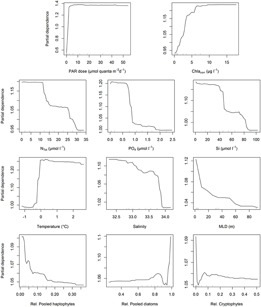
Figure 9. Partial dependence plots for all the variables included in the maximum random forest model to assess the importance of each value in the modeling op PP. The partial dependence plots for the minimal model are shown in Supplementary Figure 3. Inner tick marks represent the 10% cohorts.

Estimating Summer PP

PP over the full course of the summer season was estimated using two different approaches, the traditional M_Platt and our best RF model, M_RFmin (Figures 7, 10). Dynamics of both PP estimates were very similar (Figure 10), and both methods produced near identical values for the period after January 15th (periods 2 and 3). While the patterns in PP for December and early January (period 1) were similar, the magnitude of PP differed greatly (Figure 10). At most, PP estimated in December was a factor 2.5 higher using M_Platt than when calculated using M_RFmin. On average, M_Platt was 40% higher during the first month of the summer reaching a maximum of 6,908 mg C m⁻² d⁻¹ on December 31st (Figure 7). PP in December peaked twice in both models, namely on December 15th and 31st. After January 15th, three steep increases in PP occurred on January 21st, 30th, and February 8–12th. The maxima of these periods were of the same magnitude at those calculated for December with the M_RFmin model. In contrast, using M_Platt PP in January and February was only half of the values observed in December. A second noteworthy difference between the two methods of estimation is to which depth PP occurs (Figure 10). However, these differences contribute little to the summed PP (Figure 10). Total summer PP (Dec–Feb) was estimated to be 214.4 g C m⁻² using M_Platt and 176.1 g C m⁻² using M_RFmin, or 2.68 and 1.96 g C m⁻² d⁻¹, respectively.

FIGURE 10

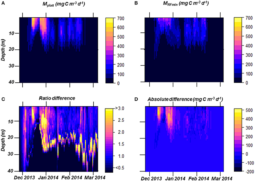
Figure 10. Estimated primary production (PP) in the top 40 m based on M_Platt (A) and on M_RFmin (B). The ratio of PP between the two models (C), values >1 indicate a higher estimates using M_Platt. This ratio is used to understand the differences in behavior between the two models. Finally, we show M_Platt minus M_RFmin (D) to present when and at which depths the two models differ or match.

Discussion

In the present study we measured PP at a coastal monitoring site over one full summer and modeled PP using two approaches (mechanistic and statistical), resulting in three different models (M_Platt, M_RFmax, and M_RFmin). Firstly, we briefly describe how our field site and the summer season dynamics were representative of the wider WAP region and conditions, both past, present and future. Then, we evaluate the M_RFmax model to find relations between environmental parameters and PP. The four most important parameters in relation to PP were PAR, phytoplankton biomass, seawater temperature and N_Tot. This full model was simplified through the reduction in parameters to obtain the minimal representative model capable of predicting PP, M_RFmin. The minimal model only included PAR, phytoplankton biomass and N_Tot. Finally, we compare both models and discuss the implications of our M_RFmin on the current efforts of modeling phytoplankton production in the coastal WAP.

From our in situ measurement, we identified four different periods during the 2013–2014 summer season (Figures 2, 4; spring, 1, 2, and 3), which were divided by the influx of large sheets of sea ice (period 1) or wind mixing events (ending periods 1 and 2). This suggests an adequate covering of past, current and future conditions in the coast WAP (Ducklow et al., 2007, 2013). Period 1 was strongly influenced by sea ice whereas 2 and 3 were not. Accurately covering of these distinctively different periods is important given the continuously decreasing expand of winter sea ice (Stammerjohn and Maksym, 2017). This summer could be classified as one of medium productivity (median summer biomass at 15 m was 4.3 μg Chl-a l⁻¹), slightly elevated SSTs and typical sea ice dynamics (Meredith et al., 2012; Venables et al., 2013; Rozema et al., 2017a). Below we briefly review the characteristics of these different periods and how these are representative for other coastal sites along the WAP to establish the range of conditions to which our models were exposed.

Influence of Presence/Absence of Sea Ice on Phytoplankton Dynamics

During period 1, the sea ice gradually melted and freshened the surface layer thereby reducing MLD and promoting diatom growth, as is typical for the traditional WAP ecosystem (Ducklow et al., 2012a, 2013). Moreover, a strong increase of turbidity indicated the marked presence of non-photosynthetic material, presumably microalgal aggregates released from the bottom of the sea ice (Figure 2B; Legge et al., 2017). Low F_v/F_m-values and relatively low values for α further suggests that the diatoms in these aggregates were low light acclimated which is typical for the sea ice environment (Table 1, Supplementary Figure 2, Arrigo et al., 2014). The difference in F_v/F_m between the late December community and the rest of the season suggests that the late December community was of a different origin, presumably the sea ice, confirming that period 1 could be deemed representative for the traditional coastal phytoplankton dynamics.

Classical features of the sea ice environment were the sole dominance of diatoms and depleted silicate stocks, the latter unexpected given the coastal nature of the site and never documented prior to the 2013–2104 summer (Clarke et al., 2008; Annett et al., 2017; Bown et al., 2017; Cassarino et al., 2017; Rozema et al., 2017b). Even though macronutrient concentrations in the water column during this period were low and uptake by phytoplankton was likely hampered, nutrients could still have been available through high bacterial remineralization, sloppy grazing, and/or viral lysis which peaks after the end of the bloom (Ducklow et al., 2012b; Brum et al., 2015). Additionally, the build-up of phytoplankton biomass could also have been ended by strong grazing, as is often observed at the sea ice edge, an attribute not covered in the RaTS program (Ross et al., 2008; Saba et al., 2014; Steinberg et al., 2015).

Brief wind mixing events marked the starts of both periods 2 and 3, two periods uninfluenced by sea ice cover. These mixing events reconfigured the water column, lower SST, and mixed the freshwater to a greater depth, thus changing the conditions for phytoplankton growth, as evident from changes in the community composition and PP. In period 2, the water column was restabilized by a fresh and shallow surface layer, which was populated by cryptophytes which are often associated with glacial meltwater (Moline et al., 2004; Saba et al., 2014). Below this layer, haptophytes and later large diatoms (mostly Proboscia spp.) thrived. Period 3 was characterized by increased wind mixing causing a more homogenous water column and deeper MLDs, typical for conditions at the end of summer and observed more frequently at the WAP (Clarke et al., 2008; Montes-Hugo et al., 2009; Venables and Meredith, 2014; Rozema et al., 2017b). Thereafter, the community consisted of large proportions of haptophytes, diatoms and cryptophytes (Figure 6).

Evaluation of Parameters Potentially Impacting PP

First and foremost, our statistical model showed the importance of light availability and biomass in the promotion of PP. While completely expected, it does establish further confidence in our statistical model, which needed to establish these relations from the training set as opposed to the mechanistic model where these relations were already established.

Nutrient concentrations during summer can be highly variable and even undetectable near the surface (Figure 5; Clarke et al., 2008; Bown et al., 2017; Rozema et al., 2017b). Governing of PP (or biomass accumulation) by macronutrients in coastal Antarctic regions have been described previously and suggested a potential limitation of nitrogen (Alderkamp et al., 2012b; Henley et al., 2017; Rozema et al., 2017b). Moreover, the nutrient dynamics are strongly influenced by the source of meltwater. Glacial melt is low in macronutrients and organic matter and dilutes the surface layer (Henley et al., 2017). This opposed to sea ice melt, a prominent source of organic matter and bacteria to remineralized the nutrients (as reviewed in Fripiat et al., 2017). Additionally, deep (wind) mixing replenishes the nutrient concentrations of the euphotic zone. These three different components control MLD in the coastal WAP system and explains why nitrogen is a better predictor for PP than MLD (Meredith et al., 2008; Rozema et al., 2017b). The positive effects of a low salinity, above 0°C water temperature and shallow MLD on PP support the importance of glacial melt in shaping the PP. But in this study, these parameters did not contribute significantly in predicting PP (Figure 8).

Moreover, our partial dependence plots suggest negative relationships between nutrient concentrations and PP (Figure 9) when above 12, 0.7, and 42 μM for N_Tot, phosphate and silicate respectively and neutral when below these thresholds. We consider these negative relations an effect from the phytoplankton community becoming dominated by only one (or at least very few) species for which the conditions are optimal when the community is blooming (Annett et al., 2010). The blooming species, which contributes most to PP, takes up most of the macro nutrients and dominates. We suspect that the blooming species draws down nutrients to concentrations in line with their uptake kinetics and half-saturation constants and, when reaching these minimum concentrations, form the plateaus in the relations between macronutrients and PP (Huisman and Weissing, 1999; Timmermans et al., 2004).

When we consider all the parameters included in our M_RFmax model, the added benefit of including phytoplankton community composition is limited (Figure 8). However, this does not imply that Chl-a specific production does not vary between the groups in the natural assemblages. The random forest model selects the parameters that explain the statistically highest possible amount of the MSE of PP. Yet, some of the variability explained by the top parameters is also be explained by mechanisms related to lower ranking parameters. Thus, while adding those parameters would not improve the model this does not mean that they are not ecologically or mechanistically important. For example, literature suggests that haptophytes favor a more unstable water column and our results confirm such a relation (Arrigo et al., 1999; Rozema et al., 2017a). However, haptophyte relative abundance is suggested to be of only minor importance in relation to PP by our models, despite a large difference between photosynthesis strategies between haptophytes and e.g., diatoms (Kropuenske et al., 2009; Alderkamp et al., 2012a). However, as we know haptophytes are related to deeper MLDs, and therefore lower SSTs, higher macronutrient concentrations and more variable PAR (Kozlowski et al., 2011; Rozema et al., 2017a). Thus, most of the variability in PP explained by knowing the fraction of haptophytes is already captured by the aforementioned parameters that rank higher. As such, we conclude that adding species information would not significantly improve models of PP in the coastal system. Sufficient knowledge of the physical, (photo)chemical properties and total phytoplankton biomass in the water column will suffice for predicting PP.

PP Estimations

Calculation of PP by both approaches (M_Platt and M_RFmin) was strongly similar except during the second half of December (Figure 10, period 1). The most important difference between these ~3 weeks and the rest of the season was the presence of melting sea ice. Estimates using M_Platt were higher (53%) during period 1 than those using M_RFmin. However, integrated biomass during period 1 was not exceptionally high when compared to period 2 or 3. In fact, it was lower than expected given the PP estimates from both models. Apparently, the high PP as measured using the P-E parameters did not result in an increase in total phytoplankton biomass. A difference in Chl-a specific production between taxonomic groups is unlikely to have been played a major role given the low contribution of taxonomic information to PP in M_RFmax (Figure 9). The large discrepancy between productivity and phytoplankton biomass accumulation could be due to a number of reasons. (1) Phytoplankton released from the sea ice are low light acclimated and were lowering their Chl-a:carbon ratio while acclimating to higher irradiance intensities in the water column, thus growth would remain undetected using Chl-a as we used Chl-a as a proxy (Sakshaug and Holm-Hansen, 1986). (2) Phytoplankton Chl-a:carbon ratios remain relatively unchanged, but the phytoplankton mainly replenish their micro- and macronutrient reserves before biomass accumulation by growth (Arrigo, 2005). These two explanations are supported by the lower F_v/F_m, possibly indicative of photo inhibition, and low α observed for this population (Table 1, Supplementary Figure 2). Additional explanations are related to ecosystems dynamics. They assume that the high productivity is translated into phytoplankton biomass, but there is also a large loss factor. (3) Sea ice occurrence is often associated with krill and other grazing which can efficiently lower phytoplankton biomass (Behrenfeld, 2010). (4) Viral lysis as after a period of biomass increase, viruses often lyse which include the bursting of phytoplankton cells and thus lowering biomass (Brum et al., 2015). Finally, the last and possibly most likely option (5) would be fast sedimentation of microalgal aggregates dominated by heavily silicified diatoms (Riebesell et al., 1991). The last three theories are supported by the observation of a very high turbidity in the surface layer (Figure 2B), not occurring elsewhere in the summer despite similar phytoplankton biomass concentrations. Our fieldwork cannot conclusively exclude any of the five hypotheses mentioned above or combinations thereof, that created the observed dynamics in phytoplankton biomass and proportions thereof to PP during period 1. Most likely it is a combination of multiple of the aforementioned explanations. Thus, while M_RFmin resembles mechanistic models that estimate PP in the marine environment, it would greatly benefit from the inclusions of parameters better explaining the phytoplankton dynamics at the sea ice edge. Also, the relation between N_Tot and PP does provide extra information for future efforts modeling PP in the coastal Antarctic ocean.

Our two estimates of 176.1 and 214.4 g C m⁻² per summer are in fair agreement with multiple different estimates of PP from previous years. Two recent estimates of net PP of 146 g C m⁻² yr⁻¹ for 2009–2010 and an estimate of 192 g C m⁻² yr⁻¹ for 2005–2006 for the RaTS site are comparable to ours (Weston et al., 2013; Henley et al., 2017). The latter estimate also employed P-E experiments with a very similar set up to ours. A slightly lower productivity of 99.4 g C m⁻² over a 5 month period was observed at a more northerly site near Palmer Station, generally considered less productive than northern Marguerite Bay (Stukel et al., 2015; Rozema et al., 2017a). Furthermore, our estimates are in broad agreement with a multi-year (1995–2006) analysis of PP using ¹⁴C along the WAP (Vernet et al., 2008). Another study based on the 2007–2008 summer but also covering the large WAP region estimate a lower productivity (78 g C m⁻² over 4 months) although this estimate is from a low biomass summer (Huang et al., 2012; Rozema et al., 2017a). Another estimate derived from calculating NCP from silica isotopes conducted at the RaTS, has calculated a maximum of only 56.4 g C m⁻² over 4 months in 2009–2010 (Annett et al., 2017). Such a large discrepancy might be related to the bias of a silica based method to diatoms as haptophytes and cryptophytes also contribute to the carbon drawdown (Figure 9) and diatom abundance was low in the 2009–2010 seasons (Rozema et al., 2017a).

Implications and Perspectives

Our data underline the importance of sea ice for phytoplankton biomass accumulation and PP in the coastal seas. Thus, a decrease in sea ice, as has been observed for the WAP since the start of the satellite record, will have substantial impact on the coastal marine system (period 1; Stammerjohn et al., 2008). Also, the diatoms associated with the sea ice and the related meltwater layer are pivotal in the food web due to the importance in the krill life cycle (Flores et al., 2012). While the loss of sea ice would result in a decrease in phytoplankton, the influence of meltwater from glaciers is rising (period 2; Moline et al., 2004; Montes-Hugo et al., 2009). While this meteoric meltwater also promotes stratification, which in turn promotes PP, the timing of the establishment of glacial meltwater layers and the phytoplankton communities within are different potentially affecting the entire food web (Moline et al., 2004; Montes-Hugo et al., 2009; Mendes et al., 2013; Saba et al., 2014; Rozema et al., 2017a). While most PP models are designed for ocean regions, the MLD at the coastal ocean is established differently than in the open ocean due to the proximity of glaciers thus are generally not adequately included in these models.

Our minimal model also underlines that dissolved nitrogen and seawater temperature can be used to estimate PP. While we do not infer a causal relation between PP and these parameters, we observe strong relation to PP. Our RF does not fully explain the dynamics in PP, namely only 93%, and we consider this is related to the dynamics occurring in December. The strong reduction in phytoplankton biomass despite a high PP suggests another source which influences phytoplankton stocks, as discussed above. We consider the counterintuitive relation between N_Tot and PP evidence of important underlying processes not captured by our accurate yet simple model. Thus, a future improvement would be the measurement and incorporation of these undescribed processes into a model. Also, the near binary effect of above and below 0°C sea surface temperatures only indicates the importance of meltwater and mixing to the winter water layer. No relation to PP was observed with increasing seawater temperature while the strength of the relation between PP and salinity declines strongly when approaching lower values (<32.5).

Conclusions

We presented a phytoplankton PP model in the highly productive northern Marguerite Bay region. We thereby considered the effect of variability in relative phytoplankton group abundances to be adequately covered by the implementation of physical and (photo)chemical properties of the water column. Firstly, we show the challenge of modeling PP in phytoplankton communities from the sea ice. This underlines the importance of the effort to obtain measurements from (below) the sea ice. Secondly, nitrogen concentrations were a stronger predictor of PP than MLD. Possibly because of the large difference in nitrogen concentrations between glacial and sea ice melt, the main sources for salinity driven stratification. Finally, our statistical models show that relative species abundances do not have to be included in future modeling efforts while maintaining a high level of confidence in the model. This last conclusion greatly simplifies the monitoring efforts required to provide field based measurements needed to estimate PP. The combination of these insights, based on both a classical, mechanistic model and independent, statistical models, should help shape the priorities for modeling efforts to accurately estimate PP in the climatically-sensitive and variable coastal WAP region.

Author Contributions

PR, GK, AB, and WvdP have designed the field experiments and protocols. MM leads the RaTS program which supplied data to this study, and helped with interpretation of the isotope data. PR has performed the field experiments and data collection. PR, MV, WvdP, and GK have designed and/or performed the data analyses. PR wrote the manuscript with input from AB and WvdP. All authors contributed to a discussion of the manuscript and approved the final outcome.

Conflict of Interest Statement

The authors declare that the research was conducted in the absence of any commercial or financial relationships that could be construed as a potential conflict of interest.

The reviewer DCLS and handling Editor declared their shared affiliation, and the handling Editor states that the process nevertheless met the standards of a fair and objective review.

Acknowledgments

We would like to thank Pim Sprong, Ronald Visser, Johann Bown and Libby Jones who have helped with the collection of the samples and data used here. Our research was made possible by and greatly benefited from all the BAS staff at Rothera and Cambridge, to whom we are very grateful. Also, we would like to thank Libby Jones for providing some of the DIC data collected by her and Hugh Venables for sharing PAR data from Rothera Research Station. Furthermore, we thank Arjo Bunskoeke and Mieke Blauw who assisted with the development, testing and implementation of the protocol for our P-E experiments. Sean de Graaf and Wendy Bollen are thanked for their help with running and processing the HPLC samples and data. This research was funded by the Dutch Polar Programme (866.10.105). Funding for the RaTS programme is from the Natural Environment Research Council, and is a component of the BAS Polar Oceans programme. Additionally, we would like to thank the editor and the reviewers for their valued opinions and suggestions which helped to improve the manuscript.

Supplementary Material

The Supplementary Material for this article can be found online at: https://www.frontiersin.org/article/10.3389/fmars.2017.00184/full#supplementary-material

References

Ærtebjerg-Nielsen, G., and Bresta, A.-M. (1984). Guidelines for the Measurement of Phytoplankton Primary Production, 2nd Edn. Baltic Marine Biologists. Charlottenlund; National Agency of Environmental Protection.

Alderkamp, A.-C., Kulk, G., Buma, A. G. J., Visser, R. J. W., van Dijken, G. L., Mills, M. M., et al. (2012a). The effect of iron limitation on the photophysiology of Phaeocystis antarctica (Prymnesiophyceae) and Fragilariopsis cylindrus (Bacillariophyceae) under dynamic irradiance. J. Phycol. 48, 45–59. doi: 10.1111/j.1529-8817.2011.01098.x

PubMed Abstract | CrossRef Full Text | Google Scholar

Alderkamp, A.-C., Mills, M. M., van Dijken, G. L., Laan, P., Thuróczy, C. E., Gerringa, L. J. A., et al. (2012b). Iron from melting glaciers fuels phytoplankton blooms in the Amundsen Sea (Southern Ocean): phytoplankton characteristics and productivity. Deep. Res. Part II Top. Stud. Oceanogr. 71–76, 32–48. doi: 10.1016/j.dsr2.2012.03.005

CrossRef Full Text | Google Scholar

Annett, A. L., Carson, D. S., Crosta, X., Clarke, A., and Ganeshram, R. S. (2010). Seasonal progression of diatom assemblages in surface waters of Ryder Bay, Antarctica. Polar Biol. 33, 13–29. doi: 10.1007/s00300-009-0681-7

CrossRef Full Text | Google Scholar

Annett, A. L., Henley, S. F., Venables, H. J., Meredith, M. P., Clarke, A., and Ganeshram, R. S. (2017). Silica cycling and isotopic composition in northern Marguerite Bay on the rapidly-warming western Antarctic Peninsula. Deep Sea Res. Part II Top. Stud. Oceanogr. 139, 132–142. doi: 10.1016/j.dsr2.2016.09.006

CrossRef Full Text | Google Scholar

Arrigo, K. R. (2005). Marine microorganisms and global nutrient cycles. Nature 437, 349–355. doi: 10.1038/nature04159

PubMed Abstract | CrossRef Full Text | Google Scholar

Arrigo, K. R., Brown, Z. W., and Mills, M. M. (2014). Sea ice algal biomass and physiology in the Amundsen Sea, Antarctica. Elem. Sci. Anthr. 2:28. doi: 10.12952/journal.elementa.000028

CrossRef Full Text | Google Scholar

Arrigo, K. R., Mills, M. M., Kropuenske, L. R., Dijken, G. L., Van Alderkamp, A., Robinson, D. H., et al. (2010). Photophysiology in two major southern ocean phytoplankton taxa: photosynthesis and growth of Phaeocystis antarctica and Fragilariopsis cylindrus under different irradiance levels. Integr. Comp. Biol. 50, 950–966. doi: 10.1093/icb/icq021

PubMed Abstract | CrossRef Full Text | Google Scholar

Arrigo, K. R., Robinson, D. H., Worthen, D. L., Dunbar, R. B., DiTullio, G. R., VanWoert, M., et al. (1999). Phytoplankton community structure and the drawdown of nutrients and CO₂ in the Southern Ocean. Science 283, 365–367. doi: 10.1126/science.283.5400.365

PubMed Abstract | CrossRef Full Text | Google Scholar

Aumont, O., Ethé, C., Tagliabue, A., Bopp, L., and Gehlen, M. (2015). PISCES-v2: an ocean biogeochemical model for carbon and ecosystem studies. Geosci. Model Dev. 8, 2465–2513. doi: 10.5194/gmd-8-2465-2015

CrossRef Full Text | Google Scholar

Behrenfeld, M., and Falkowski, P. G. (1997). A consumer's guide to phytoplankton primary productivity models. Limnol. Oceanogr. 42, 1479–1491. doi: 10.4319/lo.1997.42.7.1479

CrossRef Full Text | Google Scholar

Behrenfeld, M. J. (2010). Abandoning sverdrup's critical depth hypothesis on phytoplankton blooms critical depth hypothesis abandoning sverdrup ’ s on phytoplankton. Ecology 91, 977–989. doi: 10.1890/09-1207.1

CrossRef Full Text | Google Scholar

Bown, J., Laan, P., Ossebaar, S., Bakker, K., Rozema, P. D., and de Baar, H. J. W. W. (2017). Bioactive trace metal time series during Austral summer in Ryder Bay, Western Antarctic Peninsula. Deep Sea Res. Part II Top. Stud. Oceanogr. 139, 103–119. doi: 10.1016/j.dsr2.2016.07.004

CrossRef Full Text | Google Scholar

Breiman, L. (2001). Random Forests. Machine Learning 45, 5–32. doi: 10.1023/A:1010933404324

CrossRef Full Text | Google Scholar

Brum, J. R., Hurwitz, B. L., Schofield, O., Ducklow, H. W., and Sullivan, M. B. (2015). Seasonal time bombs: dominant temperate viruses affect Southern Ocean microbial dynamics. ISME J. 10, 1–13. doi: 10.1038/ismej.2015.125

PubMed Abstract | CrossRef Full Text | Google Scholar

Carvalho, F., Kohut, J., Oliver, M. J., and Schofield, O. (2017). Defining the ecologically relevant mixed layer depth for Antarctica's Coastal Seas. Geophys. Res. Lett. 44, 338–345. doi: 10.1002/2016GL071205

CrossRef Full Text | Google Scholar

Cassarino, L., Hendry, K. R., Meredith, M. P., Venables, H. J., and De La Rocha, C. L. (2017). Silicon isotope and silicic acid uptake in surface waters of Marguerite Bay, West Antarctic Peninsula. Deep Sea Res. Part II Top. Stud. Oceanogr. 139, 143–150. doi: 10.1016/j.dsr2.2016.11.002

CrossRef Full Text | Google Scholar

Clarke, A., Meredith, M. P., Wallace, M. I., Brandon, M. A., and Thomas, D. N. (2008). Seasonal and interannual variability in temperature, chlorophyll and macronutrients in northern Marguerite Bay, Antarctica. Deep. Res. Part II Top. Stud. Oceanogr. 55, 1988–2006. doi: 10.1016/j.dsr2.2008.04.035

CrossRef Full Text | Google Scholar

Claustre, H., Moline, M. A., and Prezelin, B. B. (1997). Sources of variability in the column photosynthetic cross section for Antarctic coastal waters. J. Geophys. Res. 102, 25047–25060. doi: 10.1029/96JC02439

CrossRef Full Text | Google Scholar

Cook, A. J., Holland, P. R., Meredith, M. P., Murray, T., Luckman, A., and Vaughan, D. G. (2016). Ocean forcing of glacier retreat in the western Antarctic Peninsula. Science 353, 283–286. doi: 10.1126/science.aae0017

PubMed Abstract | CrossRef Full Text | Google Scholar

Craig, H., and Gordon, L. (1965). “Deuterium and oxygen-18 variations in the ocean and the marine atmosphere,” in Proceedings of a Conference On Stable Isotopes In Oceanographic Studies and Paleotemperatures, ed E. Tongiorgio (Spoleto), 9–130.

Dickson, A. G., Sabine, C. L., and Christian, J. R. (2007). Guide to Best Practices for Ocean CO₂ Measurements. Sidney: North Pacific Marine Science Organization.

Google Scholar

Dierssen, H. M., and Smith, R. C. (2000). Bio-optical properties and remote sensing ocean color algorithms for Antarctic Peninsula waters. J. Geophys. Res. 105:26301. doi: 10.1029/1999JC000296

CrossRef Full Text | Google Scholar

Ducklow, H. W., Baker, K., Martinson, D. G., Quetin, L. B., Ross, R. M., Smith, R. C., et al. (2007). Marine pelagic ecosystems: the west Antarctic Peninsula. Philos. Trans. R. Soc. Lond. B Biol. Sci. 362, 67–94. doi: 10.1098/rstb.2006.1955

PubMed Abstract | CrossRef Full Text | Google Scholar

Ducklow, H. W., Clarke, A., Dickhut, R., Doney, S. C., Geisz, H., Kuan, H., et al. (2012a). The Marine System of the Western Antarctic Peninsula. Antarct. Ecosyst. An Extrem. Environ. a Chang. World, 121–159. Available online at: http://pal.lternet.edu/docs/bibliography/Public/383lterc.pdf.

Ducklow, H. W., Fraser, W. R., Meredith, M. P., Stammerjohn, S. E., Doney, S. C., Martinson, D. G., et al. (2013). West Antarctic Peninsula: an ice-dependent coastal marine ecosystem in transition. Oceanography 26, 190–203. doi: 10.5670/oceanog.2013.62

CrossRef Full Text | Google Scholar

Ducklow, H. W., Schofield, O., Vernet, M., Stammerjohn, S., and Erickson, M. (2012b). Multiscale control of bacterial production by phytoplankton dynamics and sea ice along the western Antarctic Peninsula: a regional and decadal investigation. J. Mar. Syst. 98–99, 26–39. doi: 10.1016/j.jmarsys.2012.03.003

CrossRef Full Text | Google Scholar

Flores, H., Atkinson, A., Kawaguchi, S., Krafft, B. A., Milinevsky, G., Nicol, S., et al. (2012). Impact of climate change on Antarctic krill. Mar. Ecol. Prog. Ser. 458, 1–19. doi: 10.3354/meps09831

CrossRef Full Text | Google Scholar

Fripiat, F., Meiners, K. M., Vancoppenolle, M., Papadimitriou, S., Thomas, D. N., Ackley, S. F., et al. (2017). Macro-nutrient concentrations in Antarctic pack ice : overall patterns and overlooked processes. Elem. Sci. Anthr. 5:13. doi: 10.1525/elementa.217

CrossRef Full Text | Google Scholar

Gerringa, L. J. A., Alderkamp, A.-C., Laan, P., Thuróczy, C.-E., De Baar, H. J. W., Mills, M. M., et al. (2012). Iron from melting glaciers fuels the phytoplankton blooms in Amundsen Sea (Southern Ocean): Iron biogeochemistry. Deep. Res. Part II Top. Stud. Oceanogr. 71–76, 16–31. doi: 10.1016/j.dsr2.2012.03.007

CrossRef Full Text | Google Scholar

Hammer, Ø., Harper, D. A. T., and Ryan, P. D. (2001). PAST: palaeontological statistics software package for education and data analysis. Palaeontol. Electron. 4, 1–9. doi: 10.1163/001121611X566785

CrossRef Full Text

Henley, S. F., Ganeshram, R. S., Annett, A. L., Tuerena, R. E., Fallick, A. E., Meredith, M. P., et al. (2017). Macronutrient supply, uptake and recycling in the coastal ocean of the west Antarctic Peninsula. Deep Sea Res. Part II Top. Stud. Oceanogr. 139, 58–76. doi: 10.1016/j.dsr2.2016.10.003

CrossRef Full Text | Google Scholar

Huang, K., Ducklow, H., Vernet, M., Cassar, N., and Bender, M. L. (2012). Export production and its regulating factors in the West Antarctica Peninsula region of the Southern Ocean. Global Biogeochem. Cycles 26, 1–13. doi: 10.1029/2010GB004028

CrossRef Full Text | Google Scholar

Huisman, J., and Weissing, F. J. (1999). Biodiversity of plankton by species oscillations and chaos. Nature 402, 407–410.

Google Scholar

Johnson, K. M., and Sieburth, J. M. (1987). Coulometric total carbon dioxide analysis for marine studies: automation and calibration. Mar. Chem. 21, 117–133. doi: 10.1016/0304-4203(87)90033-8

CrossRef Full Text | Google Scholar

Jones, E. M., Fenton, M., Meredith, M. P., Clargo, N. M., Ossebaar, S., Ducklow, H. W., et al. (2017). Ocean acidification and carbonate saturation states in the coastal zone of the West Antarctic Peninsula. Deep Sea Res. Part II Top. Stud. Oceanogr. 139, 181–194. doi: 10.1016/j.dsr2.2017.01.007

CrossRef Full Text | Google Scholar

Kirk, J. T. O. (1983). Light and Photosynthesis in Aquatic Ecosystems. Cambridge, UK: Cambridge University Press.

Google Scholar

Kozlowski, W. A., Deutschman, D., Garibotti, I., Trees, C., and Vernet, M. (2011). An evaluation of the application of CHEMTAX to Antarctic coastal pigment data. Deep. Res. Part I Oceanogr. Res. Pap. 58, 350–364. doi: 10.1016/j.dsr.2011.01.008

CrossRef Full Text | Google Scholar

Kropuenske, L. R., Mills, M. M., van Dijken, G. L., Bailey, S., Robinson, D. H., Welschmeyer, N. A., et al. (2009). Photophysiology in two major Southern Ocean phytoplankton taxa: photoprotection in Phaeocystis antarctica and Fragilariopsis cylindrus. Limnol. Oceanogr. 54, 1176–1196. doi: 10.4319/lo.2009.54.4.1176

CrossRef Full Text | Google Scholar

Latasa, M., Scharek, R., Vidal, M., Vila-Reixach, G., Gutiérrez-Rodríguez, A., Emelianov, M., et al. (2010). Preferences of phytoplankton groups for waters of different trophic status in the northwestern Mediterranean sea. Mar. Ecol. Prog. Ser. 407, 27–42. doi: 10.3354/meps08559

CrossRef Full Text | Google Scholar

Legge, O. J., Bakker, D. C. E., Meredith, M., Venables, H. J., and Brown, P. J. (2017). The seasonal cycle of carbonate system processes in Ryder Bay, West Antarctic Peninsula. Deep. Res. Part II. 39, 167–180. doi: 10.1016/j.dsr2.2016.11.006

CrossRef Full Text | Google Scholar

Lewis, M., and Smith, J. (1983). A small volume, short-incubation-time method for measurement of photosynthesis as a function of incident irradiance. Mar. Ecol. Prog. Ser. 13, 99–102. doi: 10.3354/meps013099

CrossRef Full Text | Google Scholar

Liaw, A., and Wiener, M. (2002). Classification and regression by random Forest. R News 2, 18–22. doi: 10.1177/154405910408300516

CrossRef Full Text | Google Scholar

MacIntyre, H. L., and Cullen, J. J. (2005). “Using cultures to investigate the physiological ecology of microalgae,” in Algal Culturing Techniques, ed R. A. Andersen (Burlington: Academic Press), 287–326.

Google Scholar

Mackey, M. D., Mackey, D. J., Higgins, H. W., and Wright, S. W. (1996). CHEMTAX - A program for estimating class abundances from chemical markers: application to HPLC measurements of phytoplankton. Mar. Ecol. Prog. Ser. 144, 265–283. doi: 10.3354/meps144265

CrossRef Full Text | Google Scholar

Marshall, G. J., Orr, A., van Lipzig, N. P. M., and King, J. C. (2006). The impact of a changing Southern Hemisphere annular mode on Antarctic peninsula summer temperatures. J. Clim. 19, 5388–5404. doi: 10.1175/JCLI3844.1

CrossRef Full Text | Google Scholar

Maxwell, K., and Johnson, G. N. (2000). Chlorophyll fluorescence–a practical guide. J. Exp. Bot. 51, 659–668. doi: 10.1093/jexbot/51.345.659

CrossRef Full Text | Google Scholar

Mendes, C. R. B., Tavano, V. M., Leal, M. C., de Souza, M. S., Brotas, V., and Garcia, C. A. E. (2013). Shifts in the dominance between diatoms and cryptophytes during three late summers in the Bransfield Strait (Antarctic Peninsula). Polar Biol. 36, 537–547. doi: 10.1007/s00300-012-1282-4

CrossRef Full Text | Google Scholar

Meredith, M. P., Brandon, M. A., Wallace, M. I., Clarke, A., Leng, M. J., Renfrew, I. A., et al. (2008). Variability in the freshwater balance of northern Marguerite Bay, Antarctic Peninsula: results from delta O-18. Deep. Res. Part II Top. Stud. Oceanogr. 55, 309–322. doi: 10.1016/j.dsr2.2007.11.005

CrossRef Full Text | Google Scholar

Meredith, M. P., and King, J. C. (2005). Rapid climate change in the ocean west of the Antarctic Peninsula during the second half of the 20th century. Geophys. Res. Lett. 32, 1–5. doi: 10.1029/2005GL024042

CrossRef Full Text | Google Scholar

Meredith, M. P., Stammerjohn, S. E., Venables, H. J., Ducklow, H. W., Martinson, D. G., Iannuzzi, R. A., et al. (2017). Changing distributions of sea ice melt and meteoric water west of the Antarctic Peninsula. Deep. Res. Part II Top. Stud. Oceanogr. 139, 40–57. doi: 10.1016/j.dsr2.2016.04.019

CrossRef Full Text | Google Scholar

Meredith, M. P., Venables, H. J., Clarke, A., Ducklow, H. W., Erickson, M., Leng, M. J., et al. (2012). The freshwater system west of the Antarctic Peninsula: spatial and temporal changes. J. Clim. 26, 1669–1684. doi: 10.1175/JCLI-D-12-00246.1

CrossRef Full Text | Google Scholar

Moline, M. A., Claustre, H., Frazer, T. K., Schofield, O., and Vernet, M. (2004). Alteration of the food web along the Antarctic Peninsula in response to a regional warming trend. Glob. Chang. Biol. 10, 1973–1980. doi: 10.1111/j.1365-2486.2004.00825.x

CrossRef Full Text | Google Scholar

Montes-Hugo, M. A., Vernet, M., Smith, R., and Carder, K. (2008). Phytoplankton size-structure on the western shelf of the Antarctic Peninsula: a remote-sensing approach. Int. J. Remote Sens. 29, 801–829. doi: 10.1080/01431160701297615

CrossRef Full Text | Google Scholar

Montes-Hugo, M., Doney, S. C., Ducklow, H. W., Fraser, W. R., Martinson, D., Stammerjohn, S. E., et al. (2009). Recent changes in phytoplankton communities associated with rapid regional climate change along the western Antarctic Peninsula. Science 323, 1470–1473. doi: 10.1126/science.1164533

PubMed Abstract | CrossRef Full Text | Google Scholar

Pebesma, E. J. (2004). Multivariable geostatistics in S: the gstat package. Comput. Geosci. 30, 683–691. doi: 10.1016/j.cageo.2004.03.012

CrossRef Full Text | Google Scholar

Perl, J. (2009). “The SDU (CHORS) method,” in The Third SeaWiFS HPLC Analysis Round-Robin Experiment (SeaHARRE-3) (NASA) (Greenbelt), 89–91.

Google Scholar

Petrou, K., Kranz, S. A., Trimborn, S., Hassler, C. S., Ameijeiras, S. B., Sackett, O., et al. (2016). Southern Ocean phytoplankton physiology in a changing climate. J. Plant Physiol. 203, 135–150. doi: 10.1016/j.jplph.2016.05.004

PubMed Abstract | CrossRef Full Text | Google Scholar

Piquet, A. M. T., Bolhuis, H., Meredith, M. P., and Buma, A. G. J. (2011). Shifts in coastal Antarctic marine microbial communities during and after melt water-related surface stratification. FEMS Microbiol. Ecol. 76, 413–427. doi: 10.1111/j.1574-6941.2011.01062.x

PubMed Abstract | CrossRef Full Text | Google Scholar

Platt, T., Gallegos, C. L., and Harrison, W. G. (1980). Photoinibition of photosynthesis in natural assemblages of marine phytoplankton. J. Mar. Res. 38, 687–701.

Google Scholar

R Core Team (2016). R: A Language and Environment for Statistical Computing. Vienna: R Foundation for Statistical Computing.

Riebesell, U., Schloss, I., and Smetacek, V. (1991). Aggregation of algae released from melting sea ice: implications for seeding and sedimentation. Polar Biol. 11, 239–248. doi: 10.1007/BF00238457

CrossRef Full Text | Google Scholar

Rignot, E., Jacobs, S., Mouginot, J., and Scheuchl, B. (2013). Ice-shelf melting around Antarctica. Science 341, 266–270. doi: 10.1126/science.1235798

PubMed Abstract | CrossRef Full Text | Google Scholar

Ross, R. M., Quetin, L. B., Martinson, D. G., Iannuzzi, R. A., Stammerjohn, S. E., and Smith, R. C. (2008). Palmer LTER: patterns of distribution of five dominant zooplankton species in the epipelagic zone west of the Antarctic Peninsula, 1993-2004. Deep. Res. Part II Top. Stud. Oceanogr. 55, 2086–2105. doi: 10.1016/j.dsr2.2008.04.037

CrossRef Full Text | Google Scholar

Rozema, P. D., Biggs, T., Sprong, P., Buma, A. G. J., Venables, H. J., Evans, C., et al. (2017a). Summer microbial community composition governed by upper-ocean stratification and nutrient availability in northern Marguerite Bay, Antarctica. Deep. Res. Part II Top. Stud. Oceanogr. 139, 151–166. doi: 10.1016/j.dsr2.2016.11.016

CrossRef Full Text | Google Scholar

Rozema, P. D., Venables, H. J., van de Poll, W. H., Clarke, A., Meredith, M. P., and Buma, A. G. J. (2017b). Interannual variability in phytoplankton biomass and species composition in northern Marguerite Bay (West Antarctic Peninsula) is governed by both winter sea ice cover and summer stratification. Limnol. Oceanogr. 62, 235–252. doi: 10.1002/lno.10391

CrossRef Full Text | Google Scholar

Saba, G. K., Fraser, W. R., Saba, V. S., Iannuzzi, R. A., Coleman, K. E., Doney, S. C., et al. (2014). Winter and spring controls on the summer food web of the coastal West Antarctic Peninsula. Nat. Commun. 5:4318. doi: 10.1038/ncomms5318

PubMed Abstract | CrossRef Full Text | Google Scholar

Sakshaug, E., and Holm-Hansen, O. (1986). Photoadaptation in Antarctic phytopfankton: variations in growth rate, chemical composition and P versus I curves. J. Plankt. Res. 8, 459–473. doi: 10.1093/plankt/8.3.459

CrossRef Full Text | Google Scholar

Schlitzer, R. (2016). Ocean Data View. Available online at: http://odv.awi.de.

Shi, T., and Horvath, S. (2006). Unsupervised learning with random forest predictors. J. Comput. Graph. Stat. 15, 118–138. doi: 10.1198/106186006X94072

CrossRef Full Text | Google Scholar

Stammerjohn, S. E., Martinson, D. G., Smith, R. C., Yuan, X., and Rind, D. (2008). Trends in Antarctic annual sea ice retreat and advance and their relation to El Niño–Southern Oscillation and Southern Annular Mode variability. J. Geophys. Res. 113, 1–20. doi: 10.1029/2007JC004269

CrossRef Full Text | Google Scholar

Stammerjohn, S., and Maksym, T. (2017). “Gaining (and losing) Antarctic sea ice: variability, trends and mechanisms,” in Sea Ice, ed D. N. Thomas (Chichester: John Wiley & Sons, Ltd), 261–289.

Google Scholar

Steeman-Nielsen, E. (1952). The Use of Radio-active Carbon (C14) for Measuring Organic Production in the Sea. ICES J. Mar. Sci. 18, 117–140.

Google Scholar

Steinberg, D. K., Ruck, K. E., Gleiber, M. R., Garzio, L. M., Cope, J. S., Bernard, K. S., et al. (2015). Long-term (1993-2013) changes in macrozooplankton off the western Antarctic peninsula. Deep. Res. Part I Oceanogr. Res. Pap. 101, 54–70. doi: 10.1016/j.dsr.2015.02.009

CrossRef Full Text | Google Scholar

Stukel, M. R., Asher, E., Couto, N., Schofield, O., Strebel, S., Tortell, P., et al. (2015). The imbalance of new and export production in the western Antarctic Peninsula, a potentially “leaky” ecosystem. Global Biogeochem. Cycles 29, 1400–1420. doi: 10.1002/2015GB005211

CrossRef Full Text | Google Scholar

Takao, S., Hirawake, T., Wright, S. W., and Suzuki, K. (2012). Variations of net primary productivity and phytoplankton community composition in the Indian sector of the Southern Ocean as estimated from ocean color remote sensing data. Biogeosciences 9, 3875–3890. doi: 10.5194/bg-9-3875-2012

CrossRef Full Text | Google Scholar

Timmermans, K. R., Wagt, B., Van Der, and de Baar, H. J. W. (2004). Growth rates, half saturation constants, and silicate, nitrate, and phosphate depletion in relation to iron availability of four large open-ocean diatoms from the Southern Ocean. Limnol. Oceanogr. 49, 2141–2151. doi: 10.4319/lo.2004.49.6.2141

CrossRef Full Text | Google Scholar

Trimborn, S., Hoppe, C. J. M., Taylor, B. B., Bracher, A., and Hassler, C. (2015). Physiological characteristics of open ocean and coastal phytoplankton communities of Western Antarctic Peninsula and Drake Passage waters. Deep. Res. Part I Oceanogr. Res. Pap. 98, 115–124. doi: 10.1016/j.dsr.2014.12.010

CrossRef Full Text | Google Scholar

Turner, J., Colwell, S. R., Marshall, G. J., Lachlan-Cope, T. A., Carleton, A. M., Jones, P. D., et al. (2005). Antarctic climate change during the last 50 years. Int. J. Climatol. 25, 279–294. doi: 10.1002/joc.1130

CrossRef Full Text | Google Scholar

Turner, J., Lu, H., White, I., King, J. C., Phillips, T., Hosking, J. S., et al. (2016). Absence of 21st century warming on Antarctic Peninsula consistent with natural variability Since the 1950s, research stations on the Antarctic Peninsula have recorded some of the largest increases in near-surface air temperature in the Southern Hemisphere. Nature 535, 411–415. doi: 10.1038/nature18645

CrossRef Full Text | Google Scholar

Turner, J., Maksym, T., Phillips, T., Marshall, G. J., and Meredith, M. P. (2013). The impact of changes in sea ice advance on the large winter warming on the western Antarctic Peninsula. Int. J. Climatol. 33, 852–861. doi: 10.1002/joc.3474

CrossRef Full Text | Google Scholar

Uitz, J., Claustre, H., Griffiths, F. B., Ras, J., Garcia, N., and Sandroni, V. (2009). A phytoplankton class-specific primary production model applied to the Kerguelen Islands region (Southern Ocean). Deep. Res. Part I Oceanogr. Res. Pap. 56, 541–560. doi: 10.1016/j.dsr.2008.11.006

CrossRef Full Text | Google Scholar

van Heukelem, L., and Thomas, C. S. (2001). Computer-assisted high-performance liquid chromatography method development with applications to the isolation and analysis of phytoplankton pigments. J. Chromatogr. A 910, 31–49. doi: 10.1016/S0378-4347(00)00603-4

PubMed Abstract | CrossRef Full Text | Google Scholar

van Leeuwe, M. A., Visser, R. J. W., and Stefels, J. (2014). The pigment composition of Phaeocystis antarctica (Haptophyceae) under various conditions of light, temperature, salinity, and iron. J. Phycol. 50, 1070–1080. doi: 10.1111/jpy.12238

PubMed Abstract | CrossRef Full Text | Google Scholar

Vaughan, D. G., Marshall, G. J., Connolley, W. M., Parkinson, C., Mulvaney, R., Hodgson, D. A., et al. (2003). Recent rapid regional climate warming on the Antarctic Peninsula. Clim. Change 60, 243–274. doi: 10.1023/A:1026021217991

CrossRef Full Text | Google Scholar

Venables, H. J., Clarke, A., and Meredith, M. P. (2013). Wintertime controls on summer stratification and productivity at the western Antarctic Peninsula. Limnol. Oceanogr. 58, 1035–1047. doi: 10.4319/lo.2013.58.3.1035

CrossRef Full Text | Google Scholar

Venables, H. J., and Meredith, M. P. (2014). Feedbacks between ice cover, ocean stratification, and heat content in Ryder Bay, western Antarctic Peninsula. J. Geophys. Res. Ocean. 119, 5323–5336. doi: 10.1002/jgrc.20224

CrossRef Full Text | Google Scholar

Vernet, M., Martinson, D., Iannuzzi, R., Stammerjohn, S., Kozlowski, W., Sines, K., et al. (2008). Primary production within the sea-ice zone west of the Antarctic Peninsula: I-Sea ice, summer mixed layer, and irradiance. Deep. Res. Part II Top. Stud. Oceanogr. 55, 2068–2085. doi: 10.1016/j.dsr2.2008.05.021

CrossRef Full Text | Google Scholar

Vernet, M., Wendy, A. K., Lynn, R. Y., Alexander, T. L., Robin, M. R., Langdon, B. Q., et al. (2012). Primary production throughout austral fall, during a time of decreasing daylength in the western Antarctic Peninsula. Mar. Ecol. Prog. Ser. 452, 45–61. doi: 10.3354/meps09704

CrossRef Full Text | Google Scholar

Weston, K., Jickells, T. D., Carson, D. S., Clarke, A., Meredith, M. P., Brandon, M., et al. (2013). Primary production export flux in Marguerite Bay (Antarctic Peninsula): linking upper water-column production to sediment trap flux. Deep. Res. Part I Oceanogr. Res. Pap. 75, 52–66. doi: 10.1016/j.dsr.2013.02.001

CrossRef Full Text | Google Scholar

Williams, C. M., Dupont, A. M., Loevenich, J., Post, A. F., Dinasquet, J., and Yager, P. L. (2016). Pelagic microbial heterotrophy in response to a highly productive bloom of Phaeocystis antarctica in the Amundsen Sea Polynya. Elem. Sci. Anthr. 4:102. doi: 10.12952/journal.elementa.000102

CrossRef Full Text | Google Scholar

Wright, S. W., Ishikawa, A., Marchant, H. J., Davidson, A. T., van den Enden, R. L., and Nash, G. V. (2009). Composition and significance of picophytoplankton in Antarctic waters. Polar Biol. 32, 797–808. doi: 10.1007/s00300-009-0582-9

CrossRef Full Text | Google Scholar

Wright, S. W., van den Enden, R. L., Pearce, I., Davidson, A. T., Scott, F. J., and Westwood, K. J. (2010). Phytoplankton community structure and stocks in the Southern Ocean (30-80°E) determined by CHEMTAX analysis of HPLC pigment signatures. Deep. Res. Part II Top. Stud. Oceanogr. 57, 758–778. doi: 10.1016/j.dsr2.2009.06.015

CrossRef Full Text | Google Scholar