Methane Production by Seagrass Ecosystems in the Red Sea

Introduction

Atmospheric methane (CH₄) is a strong greenhouse gas (Lashof and Ahuja, 1990), with a 34-fold higher global warming potential relative to the CO₂ for a time horizon of 100 years, taking in account the climate-carbon feedback (IPCC, 2013). Atmospheric CH₄ mixing ratio has more than doubled from 722 ppb in pre-industrial times to 1,803 ppb in 2011 (IPCC, 2013) with high inter-annual variability. The highest rates of CH₄ growth have been reported for the 1980's (12 ppb yr⁻¹) followed by a decrease in the 1990's (6 ppb yr⁻¹) and the lowest growth rate (2 ppb yr⁻¹) or even stabilization of CH₄ atmospheric levels in the 2000's (Dlugokencky et al., 2003; Kirschke et al., 2013). Since 2007, atmospheric CH₄ mixing ratio is increasing at high rates again (10 ppb yr⁻¹; Rigby et al., 2008). The causes of this inter-annual variability in the growth rate of CH₄ remain unclear, with difficulties in attributing this trend to specific contributions of different sources (biogenic, thermogenic, and pyrogenic emissions) and sinks (mostly, photo-oxidation by hydroxyl free radicals in the troposphere) (Bousquet et al., 2006; Kirschke et al., 2013; McNorton et al., 2016; Turner et al., 2017). The biogenic sources of methane include natural and anthropogenic emissions from wetlands, agriculture, fresh water reservoirs and oceans, ruminants, termites and organic waste.

Bottom-up estimates identify biogenic emissions from natural freshwater wetlands as the main sources of CH₄ since 1980 (Kirschke et al., 2013). In the last decade, the average global CH₄ emissions by wetlands was estimated at 190 Tg CH₄ yr⁻¹, ranging from 177 to 284 Tg CH₄ yr⁻¹ due to uncertainties mainly in coverage estimates (Kirschke et al., 2013; Melton et al., 2013). Oceanic and marine systems are also net sources of CH₄ although with lower global emissions than other sources. Yet, CH₄ emissions reported for the coastal ocean (5.5 and 1.9 Tg CH₄ yr⁻¹ for the continental shelf and estuaries, respectively; Rhee et al., 2009; EPA, 2010) exceed those reported from the open ocean (1.8 Tg CH₄ yr⁻¹; EPA, 2010), despite the coastal ocean represents < 15% of the global ocean area. The sources of CH₄ in the oceans are both biogenic, mediated by microbial processes, and thermogenic, through marine seeps. In open waters, biogenic CH₄ can be produced anaerobically by methanogens associated to particulate organic matter (Karl and Tilbrook, 1994; EPA, 2010) and aerobically as by-products during phosphonate uptake by heterotrophic bacteria under phosphate-limiting conditions (Karl et al., 2008). In coastal waters, biogenic CH₄ is mainly produced in sediments by anaerobic methanogenesis decomposing organic matter. Anaerobic methanogenesis requires anoxic conditions and redox potentials lower than −100 mV (Conrad, 2007), typically found in marine sediments (Gray, 1981). The contribution of seep and groundwater sources to CH₄ emissions in coastal waters remains unclear. Few data are available for oceanic CH₄ fluxes compared to other natural and anthropogenic sources. Oceanic CH₄ emissions were omitted in earlier assessments and have only been included in the last, the fifth, IPCC Assessment Report (IPCC, 2013), although its contribution accounts for 1–4% of the global CH₄ emissions. The paucity of data is especially important for tropical latitudes and for estuaries and shallow coastal areas, where the role of sediments colonized by seagrasses has been largely neglected. Indeed, CH₄ production rates, ranging from 5.8 to 307.2 μmol CH₄ m⁻² d⁻¹ on average, have been only reported for 4 different seagrass species in 5 locations (Table 1).

TABLE 1

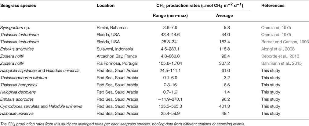
Table 1. CH₄ production rates by seagrasses reported in the literature and in this study.

Seagrass ecosystems cover shallow coastal areas from all continents, except Antarctica, with an estimated global coverage ranging from 0.15 × 10⁶ to 4.32 × 10⁶ Km² (Duarte, 2017). Thus, due to their global coverage, high productivity and high organic matter content in their sediments supporting high microbial activity compared to adjacent bare sediments, seagrass ecosystems could represent a potential important source to be included in global CH₄ budgets. Here, we report CH₄ production rates by seagrass ecosystems along the eastern Red Sea coast, encompassing 7 different species distributed across 9 locations spanning 10 degrees latitude. Moreover, in one of the seagrass meadow we measured CH₄ production rates periodically during 1 year in order to examine the existence of seasonal patterns.

Materials and Methods

We sampled 9 seagrass stations (S1–S9) along the Saudi coast of the Red Sea, onboard the R/V Thuwal on March 2017 as part of a scientific cruise covering more than 1,300 km of the Saudi Red Sea coast (Figure 1). The Red Sea is the northernmost tropical sea, reaching the 28° N parallel, with an extension of about 450,000 km² and an average depth of 490 m (Bruckner et al., 2012). Approximately 25% of its extension is occupied by shallow shelves (less than 50 m deep) holding rich and diverse marine ecosystems (Rasul et al., 2015). We sampled 7 different seagrass species: 7 stations out of the total were monospecific meadows and the other 2 were mixed meadows. Moreover, in one of the stations, an Enhalus acoroides meadow adjacent to our laboratory (S5), we also sampled periodically during 1 year, starting on June 2016 until April 2017, in order to detect seasonal patterns in CH₄ emissions.

FIGURE 1

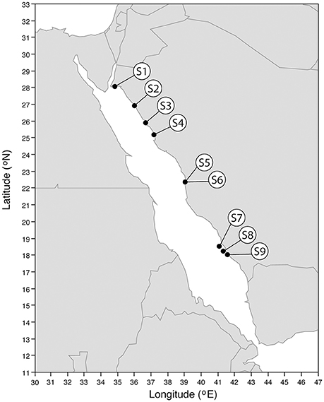
Figure 1. Location of the seagrass stations sampled along the Saudi coast of the Red Sea.

At each station and sampling event, we collected 3 or 4 replicated cylindrical plastics cores (inner diameter = 9.5 cm, height = 30 cm) containing ~10 cm of sediment (without disturbing its structure) and seagrass shots, in order to measure CH₄ production rates. We used a rubber hammer to push the plastic cores down into the sediment. The lower edges of the plastic cores were sharpened in order to facilitate the penetration of the cores into the seagrass meadow sediments. Once the core was at the desired depth into the sediment (~10 cm), we closed the upper end with a rubber cap and pulled the core up carefully, ensuring that the sediment structure was not disturbed and finally we closed immediately the lower end of the core with another rubber cap. For those stations sampled during the scientific cruise, the cores were transported immediately onboard and were secured on the upper deck in incubators equipped with a running seawater system, maintaining the temperature close to in situ temperature. For the periodical sampling events at station S5, the cores were transported immediately to the laboratory and placed in an incubator (Percival chambers) set at in situ temperature and simulating the natural photoperiod (12 h light: 12 h dark). At the end of each incubation, we collected the aboveground seagrass tissues present in each core, in order to calculate the aboveground seagrass biomass. We dried the plant material at 60°C and recorded the dry weight. Additionally, we collected 3 cores to analyze the organic matter and nutrient (C and N) content of the sediment from each station. The organic matter content was estimated by loss on ignition method, while the C and N concentration were analyzed on an CHN Elemental Analyzer (Flash 2000) after acidification of the sediment samples, in order to remove carbonates.

CH₄ Concentrations in Equilibrated Air

The concentration of CH₄ in equilibrated air along with its isotopic composition (δ¹³C-CH₄) was measured by cavity ring-down spectroscopy (Picarro G2201-i). The precision and accuracy of the CH₄ concentration analysis was ±0.01 and ±0.05 pmm, respectively. The precision and accuracy of the δ¹³C-CH₄ analysis was ±0.02 and ±1.01‰, respectively. We used an air mixture (CH₄ concentration = 9.7 ppm and CO₂ concentration = 750 ppm, Abdullah Hashim Industrial Gases & Equipment Co. Ltd., Jeddah, Saudi Arabia) as a standard for the gas concentrations and Stable Isotope Calibration Standard UN1956 (δ¹³C-CH₄ = −45‰, Air Liquide America Specialty Gases, Plumsteadville, PA, USA), as standard for the isotopic signature. We analyzed the concentration and isotopic composition of CH₄ in equilibrated air in two different setups. First, for the stations sampled during the scientific cruise and analyzed on board we used the headspace technique (section Headspace Technique: Discrete Gas Sample Analysis) and, second, for the cores collected at station S5 along 1 year we used the closed recirculating circuits technique with the cores placed in the laboratory incubation system (section Closed Recirculating Circuits: In Continuum Gas Analysis).

Headspace Technique: Discrete Gas Sample Analysis

Once on board the research vessel, the upper cap of the core was removed and seawater from the core was replaced by fresh seawater from the running surface seawater system without disturbing the sediment. Seawater temperature and salinity was recorded for further calculations. The cores were closed again with a stopper fitted with a gas-tight valve, leaving a headspace of about 250 ml. The specific volume of the sediment, seawater and headspace of each core was calculated. We left the cores to stabilize for 1 h until the first headspace sample was taken. The air sample (15 ml) from the headspace of each replicate core was withdrawn with a syringe through the gas-tight valve and the CH₄ concentration along with its isotopic composition (δ¹³C-CH₄) were analyzed immediately on board using a cavity ring-down spectrometer (Picarro G2201-i), equipped with a module for discrete small volume gas samples (Picarro Small Sample Isotope Module, SSIM A0314). Several headspace samples were taken for each core at 3–7 time intervals along the incubation and analyzed in the cavity ring-down spectrometer. The incubations lasted about 24 h for all the stations, thereby encompassing day and night periods, except for station S3 for which the incubation was extended up to 35.43 h.

Closed Recirculating Circuits: In Continuum Gas Analysis

Once the cores were settled in the incubator chamber in the laboratory, the seawater from the core was replaced by fresh seawater collected from the same location without disturbing the sediments. The cores were closed again with a stopper with two holes fitted with silicone tubbing connected to an air-water exchange module to equilibrate the gas concentration in the closed water circuit with that in the closed air circuit. The closed seawater circuit was filled with seawater, carefully removing any gas bubble. The seawater was pumped through the air-water exchange module with a peristaltic pump, recirculating the seawater from the core. The closed air circuit was connected to the cavity ring-down spectrometer (Picarro G2201-i), thereby continuously recording the CH₄ concentration in the air, equilibrated with the water circuit, along with its isotopic composition (δ¹³C- CH₄). These incubations lasted for at least 1 h, allowing net CH₄ production rates to be established, and were performed under light (200 μmol photons m⁻² s⁻¹) and dark conditions for each of the samplings.

CH₄ Concentration in Seawater

The concentration of dissolved CH₄ in seawater (in nmol CH₄ L⁻¹) was calculated from the concentration of CH₄ (in ppm) measured in air samples after equilibration from both approaches (discrete headspace samples and closed circuit in continuum) as described previously for other gases (Wilson et al., 2012). Briefly, we calculate the dissolved CH₄ remaining in seawater after equilibration with the air phase ([CH₄]_SW−eq) by,

${\left[C{H}_4\right]}_{SW-eq}={10}^{-6}\beta {\left[C{H}_4\right]}_{Air}{P}$

where β is the Bunsen solubility coefficient of CH₄, calculated according Wiesenburg and Guinasso (1979), as a function of seawater temperature and salinity; [CH₄]_Air is the CH₄ concentration measured in the air from headspace samples or closed air circuit (in ppm) and ${P}$ is the atmospheric pressure (in atm) of dry air that was corrected by the effect of multiple sampling applying Boyle's Law. Then, the initial CH₄ concentration in seawater before the equilibrium ([CH₄]_{SW−before eq}) was calculated (in ml CH₄/ml H₂O) by,

$\begin{array}{l}{\left[C{H}_4\right]}_{SW-beforeeq}=({\left[C{H}_4\right]}_{SW-eq}{V}_{Sw}+{10}^{-6}({\left[C{H}_4\right]}_{Air}\\ -{\left[C{H}_4\right]}_{Airbackground})V_{Air})/V_{SW}\end{array}$

where V_Sw is the volume of seawater in the core or in the seawater closed circuit, [CH₄]_{Air background} is the atmospheric CH₄ background level and V_Air is the volume of the headspace or the closed air circuit. Finally, the initial CH₄ concentration was transformed to nmol CH₄ L⁻¹ by applying the ideal gas law.

CH₄ Production Rates by Seagrass Meadows

CH₄ production rates (in nmol CH₄ L⁻¹ h⁻¹) were calculated based on the change in the concentration of CH₄ during the incubation time for each replicate core for each station and each sampling event. Then, we converted the rates to a daily and aerial (taking in account the core surface) base (in μmol CH₄ m⁻² d⁻¹).

Isotopic Composition (δ¹³C) of the Source CH₄

The isotopic composition (δ¹³C) of the source CH₄, i.e., CH₄ produced by seagrass ecosystems, in the Red Sea was analyzed by conducting keeling plots (Thom et al., 1993) for each of the seagrass stations sampled in this study. The δ¹³C of the source CH₄ was inferred from the Y axis intercept of the linear regression between the inverse of the CH₄ concentration measured in the equilibrated air (in ppm⁻¹) and its δ¹³C-CH₄ during our incubations.

Results

Methane production was detected at all seagrass meadows sampled, although the CH₄ emission rate varied greatly among replicates within stations and among stations (Figure 2). Some incubations reached a CH₄ concentration as high as 8,521.56 nM, (Figure 2, S6 replicate 1), whereas in others the CH₄ concentration remained very low throughout the incubation time (Figure 2, S4 replicate 2). Some incubations showed a linear increase in CH₄ concentration (Figure 2, S2 and S6), but in other incubations CH₄ concentration experienced fluctuations (Figure 2, S1 and S3), indicative of methanogenesis and methanotrophy processes. Moreover, the isotopic δ¹³C signature of CH₄ decreased when CH₄ concentration increased, confirming its biogenic origin amidst the largely thermogenic background of Red Sea waters. Conversely, the isotopic δ¹³C signature of CH₄ increased when CH₄ was oxidized by methanotrophs. The biogenic origin of the CH₄ produced in our seagrass incubations was confirmed by the δ¹³C of source CH₄, inferred from keeling plots (Figure 3). The mean δ¹³C of the CH₄ produced by seagrasses in the Red Sea was −59.36‰, ranging from −73.81 to −46.65‰ (Table 2).

FIGURE 2

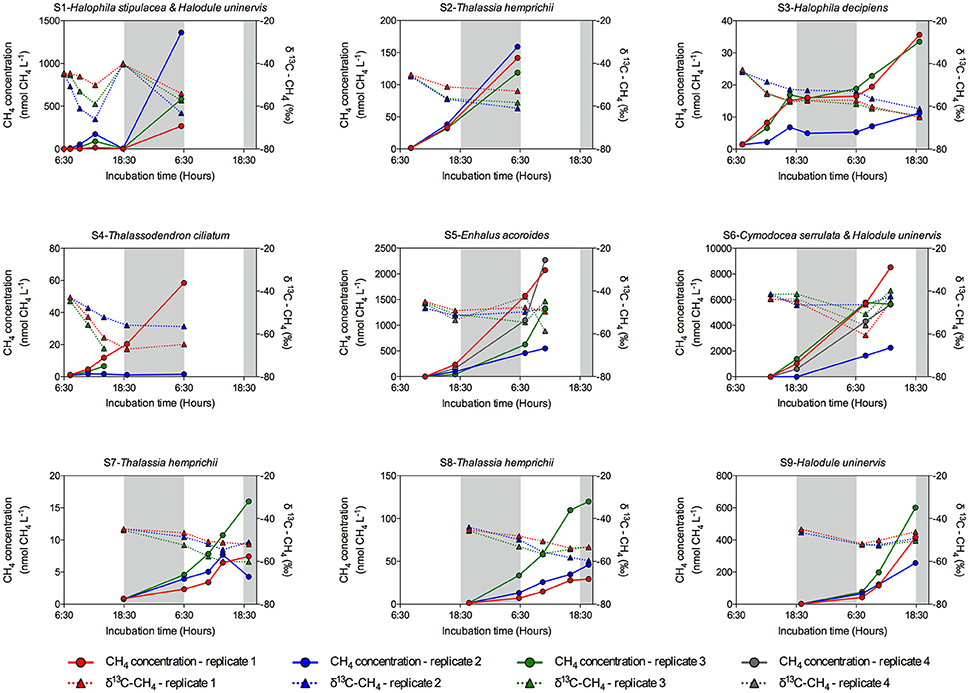
Figure 2. Evolution of CH₄ concentration (circles and solid lines) and its isotopic (δ¹³C–CH₄) signature (triangles and dashed lines) in the sediment and seagrass incubations for each seagrass station. Data from each replicate (in color code) are shown. Gray shaded area corresponds to night time. Note the different scale in Y left axis.

FIGURE 3

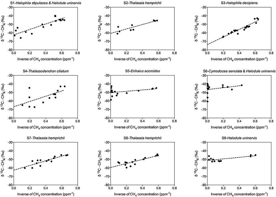
Figure 3. Keeling plots for each seagrass station, showing the linear regression fitting (dashed line) between the inverse of the CH₄ concentration and the δ¹³C–CH₄, used to calculate the isotopic signature of the source CH₄ as the intercept of Y-axis.

TABLE 2

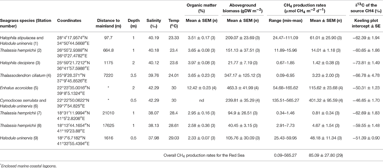
Table 2. Summary of daily CH₄ production rates (range, mean ± SEM and n) and the isotopic signature (δ¹³C) of the source CH₄ for each seagrass station, along with their location and other environmental variables.

The CH₄ production rates varied among stations, ranging from 0.09 to 565.27 μmol CH₄ m⁻² d⁻¹ (Table 2) with an overall mean of 85.09 ± 27.8 μmol CH₄ m⁻² d⁻¹ for the Red Sea seagrass meadows studied here. The lowest rates were detected in a Thalassodendron ciliatum meadow, followed by Thalassia hemprichii and Halophila decipiens meadows and the highest rates were detected in a Cymodocea serrulata and Halodule uninervis mixed meadow. The CH₄ production rates increased with sediment organic matter content (Figure 4A, R² = 0.54, p < 0.0001), and less strongly with increasing salinity (Figure 4B, R² = 0.39, p = 0.0003) and temperature (Figure 4C, R² = 0.23, p = 0.0092). The highest CH₄ production rates were observed in seagrass growing in enclosed marine coastal lagoons and the lowest rates were observed in pristine areas in shallow lagoons offshore from the mainland (Figure 4D, non-linear log fit R² = 0.54). The CH₄ production rates were independent of sediment nutrient (C and N) concentration (p = 0.77 and p = 0.25, respectively) or aboveground seagrass biomass (p = 0.11).

FIGURE 4

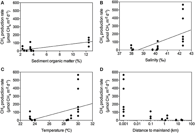
Figure 4. Linear response of CH₄ production rates to changes in sediment organic matter content (A), salinity (B) and temperature (C), showing the fitted linear model (solid line). Decline of CH₄ production rates with increasing distance from the seagrass meadow to mainland (D).

There was no evident seasonal pattern in CH₄ production rates at the Enhalus acoroides seagrass meadow (Station S5) sampled along the year, with an annually averaged daily CH₄ production rate of 92.1 ± 21.2 μmol CH₄ m⁻² d⁻¹. The CH₄ production rates measured under light and dark conditions (Figure 5A) and the daily rates (Figure 5B) did not differ among the five sampling events (ANOVA test, p = 0.43, p = 0.79, and p = 0.74, respectively). Similarly, there was no clear daily pattern in the CH₄ production rates with no tendency for rates under the light to be consistently higher or lower than those measured under dark conditions (Figure 6). The annual mean of the CH₄ production rates measured under light conditions (3.30 ± 0.92 μmol CH₄ m⁻² h⁻¹) did not differ from the annual mean of the rates measured under dark conditions (4.22 ± 0.92 μmol CH₄ m⁻² h⁻¹).

FIGURE 5

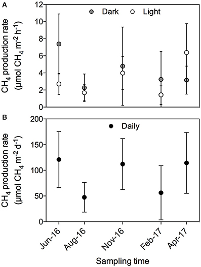
Figure 5. CH₄ production rates measured periodically during 1 year on Enhalus acoroides seagrass meadow (Station S5). (A) CH₄ production rates measured during light (open circles) and dark (gray circles) conditions. (B) Daily CH₄ production rates.

FIGURE 6

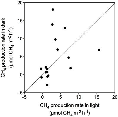
Figure 6. Relationship of CH₄ production rates measured under light and dark conditions, showing line 1:1 (dashed line).

Finally, the two different technical approaches used to measure CH₄ production rate on E. acoroides seagrass meadow (Station S5) gave similar results. The CH₄ production rate for E. acoroides using the headspace technique resulted in 115.62 ± 23.7 μmol CH₄ m⁻² d⁻¹ and the CH₄ production rate using the technique of the closed recirculating circuits for the same date resulted in 114.5 ± 59.4 μmol CH₄ m⁻² d⁻¹.

Discussion

Here, we present, for the first time, rates of CH₄ production by seagrass ecosystems in the Red Sea. The mean CH₄ production rate for the seagrass meadows analyzed in this study was 85.09 ± 27.8 μmol CH₄ m⁻² d⁻¹, ranging from 0.81 ± 0.34 to 401.32 ± 95.59 μmol CH₄ m⁻² d⁻¹ on average for a Thalassia hemprichii meadow and a Cymodocea serrulata and Halodule uninervis mixed meadow, respectively. These rates measured here are consistent with previous estimates in seagrass meadows elsewhere, with mean rates ranging from 5.8 to 307.2 μmol CH₄ m⁻² d⁻¹ for Syringodium sp. and Zostera noltii, respectively (Table 1). From all the seagrass species analyzed here, Enhalus acoroides is the only one for which CH₄ production rates were previously reported (Alongi et al., 2008), with very similar values. The CH₄ production rate reported for this seagrass in Indonesia was on average 118.8 μmol CH₄ m⁻² d⁻¹ (ranging from 4.5 to 233.1 μmol CH₄ m⁻² d⁻¹) and the rate reported here for the Red Sea was 115.6 ± 23.7 μmol CH₄ m⁻² d⁻¹ (Table 2) for the single sampling on April and 96.2 ± 17.9 μmol CH₄ m⁻² d⁻¹ when averaging the rates measured along a year (Figure 5). The high variability that we observe in our measurements has been described as well for other systems, such as freshwater wetlands (EPA, 2010).

Methane production in Red Sea seagrass meadows increased with increasing organic matter content in the sediment (Figure 4A), in agreement with previous findings of higher CH₄ concentration in porewater of seagrass sediments compared to adjacent bare sediments (Barber and Carlson, 1993). Similarly, CH₄ fluxes were more than 4-fold higher in Zostera noltii sediments compared to bare sediments in a temperate intertidal system (12.8 and 3 μmol CH₄ m⁻² h⁻¹, respectively) (Bahlmann et al., 2015), and Alongi et al. (2008) reported an increase in CH₄ release associated to an increase in seagrass productivity. Altogether, our findings and consistent literature reports suggest that organic exudates from seagrasses are fueling a complex microbial community including methanogenic Archea. Moreover, a trend toward increasing CH₄ production with increasing salinity (Figure 4B) suggests that salinity slightly enhances CH₄ production in the Red Sea, contrary to what has been previously described for estuaries and intertidal systems with freshwater inputs (Bartlett et al., 1987; Middelburg et al., 2002; Deborde et al., 2010). However, this relationship may be spurious, rather than causal, as salinity, increasing from south to north along the Red Sea, is also related to gradients in climate and productivity (Raitsos et al., 2013; Wafar et al., 2016), which may be driving the apparent relationship with salinity. Moreover, the highest salinity was observed in enclosed coastal lagoons, suggesting high rates of CH₄ production to be reached in these environments. Similarly, CH₄ production increased with seawater temperature, accounting for 25% of the variability in seagrass meadows along the Red Sea (Figure 4C). Barber and Carlson (1993) also reported the lowest values of CH₄ concentration in porewater of Thalassia testudinum sediments in Florida at 22 ^oC during winter. However, we did not detect any clear seasonal pattern in the CH₄ production for the E. acoroides meadow (Figure 5), even though the seawater temperature ranged from 22 ^oC in February to 34°C in August, during our study. This again suggest that, as for the positive relationship between salinity and CH₄ production, temperature may reflect north-south gradients in the Red Sea rather than a functional response. Similarly, we did not detect any clear diurnal patter in CH₄ production rates (Figures 2, 6). For some of our incubations, the CH₄ concentration remains stable during night time (Figure 2 S3, S7, and S9) but for others, the CH₄ concentration seems to increase faster during night time (Figure 2 S1). Our findings are in contrast with previous studies where CH₄ concentration in Thalassia testudinum rhizosphere followed diurnal cycles, with minimum values coinciding with maximum oxygen levels (Oremland and Taylor, 1977) and higher CH₄ fluxes during night in an intertidal Zostera noltii meadow (Bahlmann et al., 2015), suggesting CH₄ oxidation by photosynthetic oxygen. Part of the CH₄ produced in seagrass meadows can be oxidized before reaching the atmosphere by methanotrophic bacteria inhabiting seagrass sediments (Jones et al., 2003) consisting of an anaerobic consortium between Archea and sulfate-reducing bacteria (Boetius et al., 2000). Similarly, Oremland and Taylor (1977) found that CH₄ concentration within aerenchymatic seagrass tissues was much lower than the concentration recorded in the rhizosphere, suggesting the presence of methanotrophic bacteria inhabiting the rhizome surface. The fluctuations in CH₄ concentration and in its isotopic composition during our incubations (Figure 2), points out that both methanogenesis and methanotrophy are happening concurrently in Red Sea seagrass meadows. Bacterial methanogenesis depletes total CH₄ in ¹³C, shifting to lighter isotopic signature with respect to the starting CH₄ isotopic values, whereas CH₄ oxidation by bacteria enriches total CH₄ in ¹³C, shifting to heavier isotopic signature (Whiticar, 1990). The mean δ¹³C of the CH₄ produced by seagrasses in the Red Sea (−59.36‰) confirmed its biogenic origin. The isotopic signature of biogenic CH₄ ranges from −40 to −80‰, depending on the isotopic signature of the methanogenic substrates (Reeburgh, 2014).

Interestingly, we detected a sharp decrease in seagrass CH₄ production rates with increasing distance to the mainland, with the lowest rates detected in pristine and remote seagrass meadows (Figure 4D). Eutrophication has been related to an increase in N₂O and CH₄ production in shallow coastal areas (Bange, 2006), suggesting that further deterioration and anthropogenic disturbance on seagrass ecosystems may lead to an increase in CH₄ production and therefore CH₄ emissions. However, the Saudi Red Sea coast is relatively pristine, except for high discharges associated with main urban areas, so the reasons for the decrease in seagrass CH₄ production rates with increasing distance to the mainland remain unclear. CH₄ production rates were independent of the aboveground seagrass biomass and the C and N sediment content. The aboveground seagrass biomass varies greatly among species, depending on their size, tissue turnover and growth rate (Duarte and Chiscano, 1999). Thus, the difference in CH₄ production rates might be due to different sediment microbial communities, specific of each seagrass species.

Net fluxes or emissions to the atmosphere of the CH₄ produced by these ecosystems will depend on the solubility of CH₄ in seawater as a function of salinity and temperature, the saturation ratio (observed/equilibrium concentrations), the air-water concentration gradient and the exchange coefficient as a function of wind or turbulence (Middelburg et al., 2002). Here, we report CH₄ production rates by seagrasses, but due to the high salinity and temperatures found in the Red Sea waters that reduce the solubility of CH₄ leading to low equilibrium levels and high saturation ratios, combined with low atmospheric concentrations, we believe that the air-water concentration gradient and the prevalent winds are enough to force a significant flux of CH₄ from seawater to the atmosphere.

Assuming that the net CH₄ produced by seagrass ecosystems is emitted to the atmosphere, the CH₄ emissions of Red Sea seagrass meadows would be 19.3–70.9-fold higher, on average, than the emissions reported for the open ocean, with emissions ranging from 1.2 to 4.4 μmol m⁻² d⁻¹ (Holmes et al., 2000; Oudot et al., 2002; EPA, 2010). Moreover, taking in account the range of global estimates for seagrass coverage, from 0.15 × 10⁶ to 4.32 × 10⁶ Km² (Duarte, 2017) and using the mean seagrass CH₄ production rate calculated by compounding our estimates with those available in the literature (105.8 ± 34.4 μmol CH₄ m⁻² d⁻¹), the global CH₄ production and emission by seagrass ecosystems could range from 0.09 to 2.7 Tg yr⁻¹. Because CH₄ emission by seagrass ecosystems had not been included in previous global estimates, the estimate provided here would increase the contribution of marine global emissions, hitherto estimated at 9.1 Tg yr⁻¹ (EPA, 2010), by about 30%. In terms of CO₂-equivalents, calculated with the global warming potential for a time horizon of 100 years taking in account the climate-carbon feedback (IPCC, 2013), the CH₄ emissions by seagrass ecosystems would represent 3.2–90.9 Tg CO_2−eq yr⁻¹. This would imply a modest, 4.8%, reduction in the carbon sink capacity of seagrass ecosystems, estimated between 65.5 and 1,887.5 Tg CO₂ yr⁻¹ for the lower and upper limit of the seagrass coverage range (Duarte et al., 2010). However, these estimates are tentative for both the regional variation in CH₄ emissions by seagrass ecosystems and the poorly constrained global seagrass area. In any case, the first order estimate of potential contribution of seagrass ecosystems to marine CH₄ emissions provides sufficient evidence of the relevance of these fluxes as to include seagrass ecosystems in future assessments of the global CH₄ budgets.

Author Contributions

NG-B and CD designed the study and collected samples. NG-B acquired and analyzed the data. NG-B and CD interpreted data, wrote and reviewed the manuscript.

Conflict of Interest Statement

The authors declare that the research was conducted in the absence of any commercial or financial relationships that could be construed as a potential conflict of interest.

The reviewer MKD and handling Editor declared their shared affiliation.

Acknowledgments

This research was supported by King Abdullah University of Science and Technology (KAUST) through the baseline fund to CD. We thank Paloma Carrillo de Albornoz for her assistance during field and laboratory work. We also thank the crew of R/V Thuwal for their assistance in our field work during the scientific cruise.

References

Alongi, D. M., Trott, L. A., Undu, M. C., and Tirendi, F. (2008). Benthic microbial metabolism in seagrass meadows along a carbonate gradient in Sulawesi, Indonesia. Aquat. Microb. Ecol. 51, 141–152. doi: 10.3354/ame01191

CrossRef Full Text | Google Scholar

Bahlmann, E., Weinberg, I., Lavrič, J., Eckhardt, T., Michaelis, W., Santos, R., et al. (2015). Tidal controls on trace gas dynamics in a seagrass meadow of the Ria Formosa lagoon (southern Portugal). Biogeosciences 12, 1683–1696. doi: 10.5194/bg-12-1683-2015

CrossRef Full Text | Google Scholar

Bange, H. W. (2006). Nitrous oxide and methane in European coastal waters. Estuarine Coastal Shelf Sci. 70, 361–374. doi: 10.1016/j.ecss.2006.05.042

CrossRef Full Text | Google Scholar

Barber, T. R., and Carlson, P. R. (1993). “Effects of seagrass die-off on benthic fluxes and porewater concentrations of ∑CO₂, ∑H₂S, and CH₄ in florida bay sediments,” in Biogeochemistry of Global Change, ed R. S. Oremland (Boston, MA: Springer), 530–550. doi: 10.1007/978-1-4615-2812-8_29

CrossRef Full Text | Google Scholar

Bartlett, K. B., Bartlett, D. S., Harriss, R. C., and Sebacher, D. I. (1987). Methane emissions along a salt marsh salinity gradient. Biogeochemistry 4, 183–202. doi: 10.1007/BF02187365

CrossRef Full Text | Google Scholar

Boetius, A., Ravenschlag, K., Schubert, C. J., and Rickert, D. (2000). A marine microbial consortium apparently mediating anaerobic oxidation of methane. Nature 407:623. doi: 10.1038/35036572

PubMed Abstract | CrossRef Full Text | Google Scholar

Bousquet, P., Ciais, P., Miller, J. B., Dlugokencky, E. J., Hauglustaine, D. A., Prigent, C., et al. (2006). Contribution of anthropogenic and natural sources to atmospheric methane variability. Nature 443, 439–443. doi: 10.1038/nature05132

PubMed Abstract | CrossRef Full Text | Google Scholar

Bruckner, A., Rowlands, G., Riegl, B., Purkis, S. J., Williams, A., and Renaud, P. (2012). Khaled bin Sultan Living Oceans Foundation Atlas of Saudi Arabian Red Sea Marine Habitats. Phoenix, AZ: Panoramic Press.

Google Scholar

Conrad, R. (2007). Microbial ecology of methanogens and methanotrophs. Adv. Agron. 96, 1–63. doi: 10.1016/S0065-2113(07)96005-8

CrossRef Full Text | Google Scholar

Deborde, J., Anschutz, P., Guérin, F., Poirier, D., Marty, D., Boucher, G., et al. (2010). Methane sources, sinks and fluxes in a temperate tidal Lagoon: the Arcachon lagoon (SW France). Estuarine Coastal Shelf Sci. 89, 256–266. doi: 10.1016/j.ecss.2010.07.013

CrossRef Full Text | Google Scholar

Dlugokencky, E. J., Houweling, S., Bruhwiler, L., Masarie, K. A., Lang, P. M., Miller, J. B., et al. (2003). Atmospheric methane levels off: temporary pause or a new steady-state? Geophys. Res. Lett. 30:1992. doi: 10.1029/2003GL018126

CrossRef Full Text | Google Scholar

Duarte, C. M. (2017). Reviews and syntheses: hidden forests, the role of vegetated coastal habitats in the ocean carbon budget. Biogeosciences 14:301. doi: 10.5194/bg-14-301-2017

CrossRef Full Text | Google Scholar

Duarte, C. M., and Chiscano, C. L. (1999). Seagrass biomass and production: a reassessment. Aquat. Bot. 65, 159–174. doi: 10.1016/S0304-3770(99)00038-8

CrossRef Full Text | Google Scholar

Duarte, C. M., Marbà, N., Gacia, E., Fourqurean, J. W., Beggins, J., Barrón, C., et al. (2010). Seagrass community metabolism: assessing the carbon sink capacity of seagrass meadows. Global Biogeochem. Cycles 24:GB4032. doi: 10.1029/2010GB003793

CrossRef Full Text | Google Scholar

EPA (2010). Methane and Nitrous Oxide Emissions from Natural Sources, eds B. Anderson, K. Bartlett, S. Frolking, K. Hayhoe, J. Jenkins and W. Salas. Washington, DC: Environmental Protection Agency.

Gray, J. S. (1981). The Ecology of Marine Sediments. New York, NY: Cambridge University Press.

Google Scholar

Holmes, M. E., Sansone, F. J., Rust, T. M., and Popp, B. N. (2000). Methane production, consumption, and air-sea exchange in the open ocean: an evaluation based on carbon isotopic ratios. Global Biogeochem. Cycles 14, 1–10. doi: 10.1029/1999GB001209

CrossRef Full Text | Google Scholar

IPCC (2013). Climate change 2013: The Physical Science Basis. Contribution of Working Group I to the Fifth Assessment Report (AR5) of the Intergovernmental Panel on Climate Change. New York, NY: Cambridge University Press.

Jones, W. B., Cifuentes, L. A., and Kaldy, J. E. (2003). Stable carbon isotope evidence for coupling between sedimentary bacteria and seagrasses in a sub-tropical lagoon. Mar. Ecol. Progr. Ser. 255, 15–25. doi: 10.3354/meps255015

CrossRef Full Text | Google Scholar

Karl, D. M., Beversdorf, L., Björkman, K. M., Church, M. J., Martinez, A., and Delong, E. F. (2008). Aerobic production of methane in the sea. Nat. Geosci. 1, 473–478. doi: 10.1038/ngeo234

CrossRef Full Text | Google Scholar

Karl, D. M., and Tilbrook, B. D. (1994). Production and transport of methane in oceanic particulate organic matter. Nature 368, 732–734. doi: 10.1038/368732a0

CrossRef Full Text | Google Scholar

Kirschke, S., Bousquet, P., Ciais, P., Saunois, M., Canadell, J. G., Dlugokencky, E. J., et al. (2013). Three decades of global methane sources and sinks. Nat. Geosci. 6, 813–823. doi: 10.1038/ngeo1955

CrossRef Full Text | Google Scholar

Lashof, D. A., and Ahuja, D. R. (1990). Relative contributions of greenhouse gas emissions to global warming. Nature 344, 529–531. doi: 10.1038/344529a0

CrossRef Full Text | Google Scholar

McNorton, J., Chipperfield, M. P., Gloor, M., Wilson, C., Feng, W., Hayman, G. D., et al. (2016). Role of OH variability in the stalling of the global atmospheric CH 4 growth rate from 1999 to 2006. Atmos. Chem. Phys. 16, 7943–7956. doi: 10.5194/acp-16-7943-2016

CrossRef Full Text | Google Scholar

Melton, J., Wania, R., Hodson, E., Poulter, B., Ringeval, B., Spahni, R., et al. (2013). Present state of global wetland extent and wetland methane modelling: conclusions from a model intercomparison project (WETCHIMP). Biogeosciences 10, 753–788. doi: 10.5194/bg-10-753-2013

CrossRef Full Text | Google Scholar

Middelburg, J. J., Nieuwenhuize, J., Iversen, N., Høgh, N., De Wilde, H., Helder, W., et al. (2002). Methane distribution in European tidal estuaries. Biogeochemistry 59, 95–119. doi: 10.1023/A:1015515130419

CrossRef Full Text | Google Scholar

Oremland, R. S. (1975). Methane production in shallow-water, tropical marine sediments. Appl. Microbiol. 30, 602–608.

PubMed Abstract | Google Scholar

Oremland, R. S., and Taylor, B. F. (1977). Diurnal fluctuations of O2, N2, and CH4 in the rhizosphere of Thalassia testudinum. Limnol. Oceanogr. 22, 566–570. doi: 10.4319/lo.1977.22.3.0566

CrossRef Full Text | Google Scholar

Oudot, C., Jean-Baptiste, P., Fourré, E., Mormiche, C., Guevel, M., Ternon, J.-F., et al. (2002). Transatlantic equatorial distribution of nitrous oxide and methane. Deep Sea Res. Part I Oceanogr. Res. Pap. 49, 1175–1193. doi: 10.1016/S0967-0637(02)00019-5

CrossRef Full Text | Google Scholar

Raitsos, D. E., Pradhan, Y., Brewin, R. J. W., Stenchikov, G., and Hoteit, I. (2013). Remote sensing the phytoplankton seasonal succession of the Red Sea. PLoS ONE 8:e64909. doi: 10.1371/journal.pone.0064909

PubMed Abstract | CrossRef Full Text | Google Scholar

Rasul, N. M. A., Stewart, I. C. F., and Nawab, Z. A. (2015). “Introduction to the Red Sea: its origin, structure, and environment,” in The Red Sea: The Formation, Morphology, Oceanography and Environment of a Young Ocean Basin, eds N. M. A. Rasul and I. C. F. Stewart (Berlin; Heidelberg: Springer Berlin Heidelberg), 1–28.

Google Scholar

Reeburgh, W. S. (2014). “Global methane biogeochemistry,” in Treatise on Geochemistry, 2nd Edn, eds H. D. Holland and K. K. Turekian (Oxford: Elsevier), 71–94.

Google Scholar

Rhee, T. S., Kettle, A. J., and Andreae, M. O. (2009). Methane and nitrous oxide emissions from the ocean: a reassessment using basin-wide observations in the Atlantic. J. Geophys. Res. 114:D12304. doi: 10.1029/2008JD011662

CrossRef Full Text | Google Scholar

Rigby, M., Prinn, R. G., Fraser, P. J., Simmonds, P. G., Langenfelds, R. L., Huang, J., et al. (2008). Renewed growth of atmospheric methane. Geophys. Res. Lett. 35:L22805. doi: 10.1029/2008GL036037

CrossRef Full Text | Google Scholar

Thom, M., Bösinger, R., Schmidt, M., and Levin, I. (1993). The regional budget of atmospheric methane of a highly populated area. Chemosphere 26, 143–160. doi: 10.1016/0045-6535(93)90418-5

CrossRef Full Text | Google Scholar

Turner, A. J., Frankenberg, C., Wennberg, P. O., and Jacob, D. J. (2017). Ambiguity in the causes for decadal trends in atmospheric methane and hydroxyl. Proc. Nat. Acad. Sci. U.S.A. 114, 5367–5372. doi: 10.1073/pnas.1616020114

PubMed Abstract | CrossRef Full Text | Google Scholar

Wafar, M., Qurban, M. A., Ashraf, M., Manikandan, K., Flandez, A. V., and Balala, A. C. (2016). Patterns of distribution of inorganic nutrients in Red Sea and their implications to primary production. J. Mar. Syst. 156, 86–98. doi: 10.1016/j.jmarsys.2015.12.003

CrossRef Full Text | Google Scholar

Whiticar, M. J. (1990). A geochemial perspective of natural gas and atmospheric methane. Org. Geochem. 16, 531–547. doi: 10.1016/0146-6380(90)90068-B

CrossRef Full Text | Google Scholar

Wiesenburg, D. A., and Guinasso, N. L. (1979). Equilibrium solubilities of methane, carbon monoxide, and hydrogen in water and sea water. J. Chem. Eng. Data 24, 356–360. doi: 10.1021/je60083a006

CrossRef Full Text | Google Scholar

Wilson, S. T., Böttjer, D., Church, M. J., and Karl, D. M. (2012). Comparative assessment of nitrogen fixation methodologies, conducted in the oligotrophic North Pacific Ocean. Appl. Env. Microbiol. 78, 6516–6523. doi: 10.1128/AEM.01146-12

PubMed Abstract | CrossRef Full Text | Google Scholar