Trends in Primary Production in the Canary Current Upwelling System—A Regional Perspective Comparing Remote Sensing Models

Introduction

Over recent decades increasing trends in global warming have been evident in most oceanic regions, both at surface and deep layers (Levitus et al., 2000, 2005; Gille, 2002; Ihara et al., 2008; Hansen et al., 2010; Gouretski et al., 2012; Nieves et al., 2015). Impacts of rising temperatures on marine ecosystems may have direct effects on the ranges of distribution and vulnerability of organisms, but also on the productivity of ecosystems, their management and their services (Aalst et al., 2014). Ocean surface warming leads to enhanced stratification of the water column, reducing vertical mixing and hence limiting the supply of colder, nutrient-enriched waters to the euphotic zone, where primary production takes place. Behrenfeld et al. (2006) were the first to provide evidence of a reduction on global average net primary production (NPP), derived from remote sensing ocean-color data, of 190 TgC·year⁻¹ for the 1999–2006 period, associated with a global warming trend during the same period. Boyce et al. (2010) combined in situ chlorophyll a (Chl-a) measurements with sea water transparency to found also a global significant decline of Chl-a (about −0.020 mg·m⁻³·°C⁻¹) over the twentieth century, related to increasing sea surface temperatures (SST). Nevertheless, other authors have found both increasing and decreasing trends on phytoplankton biomass and primary productivity, related to multi-decadal climatic oscillations over the last century, showing variable regional patterns (Martinez et al., 2009; Chavez et al., 2011). Overall, present observations suggest that NPP will increase with global warming at high latitudes, but this enhancement will be offset by a decrease in the open-ocean at temperate and tropical latitudes (Behrenfeld et al., 2006; Martinez et al., 2009; Chavez et al., 2011). Moreover, the poor and uncertain information on the productivity trends at coastal and near-shore regions, which largely contribute to the global productivity, reduce confidence in future global projections (Aalst et al., 2014). Indeed, although the global ocean is projected to warm under climate change, the surface waters of eastern boundary upwelling ecosystems (EBUE)—contributing nearly 25% to global fish production—may lead to cooling rather than warming, causing enhanced productivity. Bakun (1990) proposed that EBUEs would tend to cool, as the result of the intensification of wind-driven upwelling. According to his hypothesis, the stronger continental land mass warming compared to the ocean would cause an increase in the cross-shore atmospheric pressure gradient, intensifying coastal upwelling, hence enhancing primary productivity. Analyses of sea-surface temperatures, wind trends and chlorophyll provide however contradictory evidences to support Bakun's hypothesis in all EBUEs (Snyder et al., 2003; McGregor et al., 2007; Demarcq, 2009; Narayan et al., 2010; Barton et al., 2013; Cropper et al., 2014; Sydeman et al., 2014; Oerder et al., 2015; Varela et al., 2015; Wang et al., 2015). Moreover, it is unclear to what extent wind stress can offset the increased stratification in upwelling regions due to surface warming, and how other ecosystem drivers (like the progressive acidification and deoxygenation) could affect organisms' responses and ecosystem productivity in EBUEs.

The present work aims to shed some light on this controversy by analyzing spatiotemporal trends on physical and biological variables in the Canary Current (CanC) upwelling region, which is located along the northwestern African coast (Figure 1) and constitutes one of the four major EBUEs in the planet, along with the California, Humboldt and Benguela systems (Carr and Kearns, 2003; Chavez and Messié, 2009). We use satellite data to explore seasonal to interannual trends in sea-surface temperature, chlorophyll and primary production, for the 1998–2015 period. Past observations indicate that the CanC has been warming at both local and regional scales since the early 1980s, with a decrease in chlorophyll over the last two decades (Arístegui et al., 2009; Belkin, 2009; Demarcq, 2009). In this study we have further extended the analyses to sub-regional scales and introduce a trend analysis on NPP employing various well-known models, an effort that had not being done yet for this upwelling system.

FIGURE 1

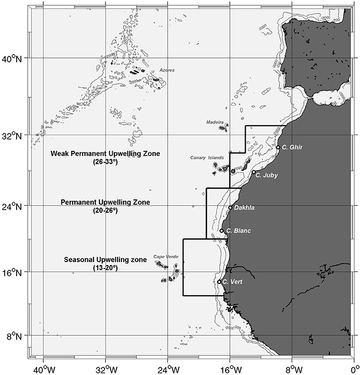
Figure 1. CanC upwelling region and its main geographical features. The three upwelling subregions –the weak permanent (WPUZ), permanent (PUZ), and seasonal upwelling zones (SUZ)– are identified along with the geographical domains selected to estimate climatological anomalies (black boxes). 200 m and 2,000 m isobaths are represented by gray contour lines. Bathymetry data corresponds to a 2′ global dataset derived by Smith and Sandwell (1997).

Data and Methods

Study Area

Although the large marine ecosystem of the CanC, in its broadest sense, spans from the northwest tip of the Iberian Peninsula to south of Senegal (Arístegui et al., 2009), we refer here to the CanC region as the area extending from northern Morocco to Senegal. The CanC constitutes the eastern boundary of the North Atlantic subtropical gyre and flows parallel to the Northwest African continental margin until ~15–21°N, where it detaches from the coast and merges into the westward North Equatorial Current (NEC). The CanC region displays a great geographical variability, resulting in highly diverse upwelling environments (Arístegui et al., 2009). For instance, the nutrient content of upwelled waters differs depending on the source of the water mass: North Atlantic Central Waters (NACW) and South Atlantic Central Waters (SACW) dominate north and south of Cape Blanc (21°N), respectively, with SACW providing higher concentrations of nutrients than the NACW. Mesoscale activity plays also an important role in upwelling dynamics, as changes in shelf width and the presence of capes (e.g., Capes Ghir, Juby, and Bojador) enhance the formation of recurrent filaments that export organic matter from the upwelling into the oligotrophic waters of the North Atlantic subtropical gyre. Besides, the perturbation of the main flow by the Canary Archipelago induces the generation of mesoscale eddies downstream the islands (at about 27–28°N), many of them drifting westwards to the open ocean along the path of an “eddy corridor” (Sangrà et al., 2009). Dust deposition is also a major feature, especially in the southern part of the study area, as the transport of mineral aerosols from the Sahara desert and the Sahel makes the CanC one of the regions with the highest dust deposition rates in the world (Mahowald et al., 2005). Despite this high diversity of environments, three main sub-regions are identified for the purpose of this study according to their upwelling intensity throughout the year, based on previous regional descriptions (Wooster et al., 1976; Van Camp et al., 1991; Cropper et al., 2014): a seasonal upwelling zone (SUZ) along the Senegalese-Mauritanian coast, which expands from 13 to 20°N, a permanent upwelling zone (PUZ), from 20 to 26°N, and a weak permanent upwelling zone (WPUZ), from 26 to 33°N (Figure 1). Notice, however, that these latitudinal bands represent approximate boundaries, as in practice they might vary from year to year due to the meridional shift of the trade wind system. While the WPUZ and PUZ present year-round upwelling (peaking during summer in the northern section), the SUZ exhibits winter upwelling followed by a downwelling period, especially during summer months, due to the appearance of the onshore monsoonal winds.

Sea-Surface Temperature (SST)

SST from daily Reynolds analyses that combine AVHRR and in situ data (at a weekly temporal and 1/4° spatial resolutions) was provided by the Copernicus Marine Environment Monitoring Service (CMEMS, http://marine.copernicus.eu/), product reference GLOBAL_REP_PHYS_001_013. The dataset covers the period from 01/1993 to 12/2014.

Net Primary Production (NPP)

The main goal of this study is to look at seasonal to decadal trends in productivity in the CanC region. For this purpose three well-known NPP models are selected to compare them: the VGPM, the Eppley-VGPM and the CbPM (r2014), all three provided by the Oregon State University (OSU, http://www.science.oregonstate.edu/ocean.productivity/) with temporal and spatial resolutions of 8 days and 1/12°, respectively. In order to study the longest possible time period, we employ data derived both from SeaWiFS and MODIS; the former expands the 01/1998–12/2007 period, whereas the latter the 01/2003–12/2015 one.

The VGPM is a Chl-based model developed by Behrenfeld and Falkowski (1997). Using chl-a as a biomass proxy, it estimates NPP as a function of the maximum daily net primary production found within a given water column (${\text{P}}_{\text{opt}}^{\text{B}}$), which is intended to represent the variation of light-saturated photosynthetic efficiencies. The ${\text{P}}_{\text{opt}}^{\text{B}}$ is defined by a complex empirical, SST-dependent polynomial expression of 7th degree:

$\begin{array}{l}{P}_{opt}^B=-3.27·{10}^{-8}{T}^7+3.4132·{10}^{-6}{T}^6-1.348·{10}^{-4}{T}^5\\ +2.462·{10}^{-3}{T}^4-0.0205T^3+0.0617T^2\\ +0.2749T+1.2956\end{array}$

Estimates are integrated to the whole water column by a volume function that depends on the depth of the euphotic zone (z_eu) and a term that accounts for the vertical decrease in light (as photosynthetically active radiation, PAR), which is empirically parametrized. Thus, multiplying by the daily hours of light (h_PAR) the following expression is obtained:

$\begin{array}{l}NPP=chl·P_{opt}^B·h_{PAR}·\left[0.66125·\frac{PAR}{PAR+4.1}\right]·z_{eu}\end{array}$

The Eppley-VGPM represents a modified version of the VGPM, replacing the original polynomial description of ${\text{P}}_{\text{opt}}^{\text{B}}$ with the exponential function described by Morel (1991), based on the curvature of the temperature-dependent growth function of Eppley (1972):

$\begin{array}{l}{P}_{opt}^B=1.54·{10}^{0.0275·SST-0.07}\end{array}$

The CbPM was developed by Behrenfeld et al. (2005) and modified by Westberry et al. (2008). The key difference from the previous two models is that instead of considering chl-a as a proxy of phytoplankton biomass it employs organic carbon estimates. Phytoplankton carbon (C_phyto) is calculated from an empirical relationship that relates it to the particulate backscattering coefficient (b_bp):

$\begin{array}{l}{C}_{phyto}=13000·\left(b_{bp}-0.00035\right)\end{array}$

The chosen physiological rate was phytoplankton growth (μ), which is estimated based on chl:C ratios:

$\begin{array}{l}\mu =\mu {}_{max}·\left[\frac{chl:C_{sat}-\epsilon }{chl:C_{N,T_{max}}-\epsilon }\right]·\left[1-e^{-5I}\right]\end{array}$

where μ_max is the maximum growth rate (set at 2 div·day⁻¹ after Banse, 1991), chl:C_sat are the observed satellite-derived chl:C ratios and ε is the intercept between chl:C and μ. Chl:C ratios under nutrient replete conditions (chl:C_N,Tmax) were empirically parametrized. Besides, the modified version of the CbPM includes a modification of chl:C ratios for depths under the nitracline. The last term accounts for the light-dependent growth. See Westberry et al. (2008) for details.

Finally, light change through the water column is parametrized as follows:

$\begin{array}{l}{I}_g=I_0·e^{\frac{-k_{490}·MLD}{2}}\end{array}$

where I₀ is cloud-corrected surface PAR, k₄₉₀ the light attenuation coefficient at 490 nm and MLD the mixed layer depth.

Thus, CbPM NPP is given by the product of the three terms:

$\begin{array}{l}NPP=C_{phyto}·\mu ·I_g\end{array}$

Chlorophyll-a (Chl-a)

Chl-a was provided by the European Space Agency (ESA) through the Ocean Colour–Climate Change Initiative (OC–CCI) portal (http://esa-oceancolour-cci.org/) with a temporal resolution of 8 days and 4 km² spatial resolution (v3.1) for the 1998–2015 period. This product consists in globally merged data from MERIS (MEdium Resolution Imaging Spectrometer), Aqua-MODIS, SeaWiFS and VIIRS (Visible Infrared Imaging Radiometer Suite), contributing to the reduction of cloud cover and bias correction. Besides, the individual datasets of SeaWiFS and MODIS Chl-a employed in the NPP estimates were downloaded from the OSU portal. Chl-a is usually employed as a proxy for phytoplankton biomass, although it is worth to note that the “carbon:Chl-a ratio” may vary among different species of phytoplankton as well as their metabolic states.

Linear Fits

Linear fits are computed in order to estimate the change rate of the different variables throughout the time period analyzed. The Theil-Sen slope estimator was chosen for this purpose, since it is a robust method against outliers that generate departures from normality and homoscedasticity of the residuals. The method, developed by Theil (1950) and later extended by Sen (1968), yields a simple linear regression of a set of data points, estimating the median slope among all lines connecting pairs of points. Although it is a robust method, correction for temporal autocorrelation is required to correctly estimate the significance of the calculated slopes. This is achieved making use of the modified Mann-Kendall trend test developed by Hamed and Ramachandra Rao (1998), which corrects Mann-Kendall test Z statistics and, consequently, p-values for autocorrelated data. The significance boundary is set at the usual 0.05 level.

Correlations

As datasets in the present work exhibit departures from normality and extreme values, we use the Spearman's rank correlation coefficient (also known as Spearman's ρ), a non-parametric method that is robust to outliers. The significance boundary chosen was the usual 0.05 level.

Seasonal Climatological Anomalies

Seasonal climatological anomalies are estimated within each upwelling subregion to better study fluctuations of the different variables and thus support the trend analysis. The selected areas are shown in Figure 1. The box approach is chosen taking into account the different spatial resolution of some of the datasets, and in order to include the oceanward extensions of the coastal upwelling.

The procedure followed for their computation involves three steps: (1) Averaging datasets in order to obtain seasonal time series, dividing each year into four quarters: (i) winter, corresponding to January, February and March (JFM); (ii) spring, corresponding to April, May and June (AMJ); (iii) summer, corresponding to July, August and September (JAS); and (iv) autumn, corresponding to October, November and December (OND); (2) Calculating mean values for each season, i.e., seasonal climatologies (this is done independently for each sensor's time-series); and (3) Subtracting the corresponding seasonal climatology from each measured seasonal value. In order to estimate the anomalies for all the three upwelling subregions, datasets are also spatially averaged prior to the computation of climatologies.

Climate Indices

Five climate indices are selected to look at correlations with the studied variables:

The Multivariate ENSO Index (MEI) and the Southern Oscillation Index (SOI). Although MEI and SOI both describe the El Niño-Southern Oscillation (ENSO) they do it in distinct ways: while SOI is based on the observed sea-level pressure (SLP) differences between Tahiti and Darwin (Australia), MEI takes six observed variables into account: SLP, zonal, and meridional components of the surface wind, SST, surface air temperature and total cloudiness fraction of the sky. Despite the fact that MEI and SOI characterize the same phenomena both are analyzed in order to make stronger assumptions supported by two different indices. Both MEI and SOI were provided by the National Oceanic and Atmospheric Administration (NOAA) at http://www.esrl.noaa.gov/psd/enso/mei/ and https://www.ncdc.noaa.gov/teleconnections/enso/indicators/soi/, respectively.

The station-based North Atlantic Oscillation (NAO-SB) and the principal component-based North Atlantic Oscillation (NAO-PC). The NAO-SB is based on the difference of normalized SLP between Lisbon (Portugal) and Stykkisholmur/Reykjavik (Iceland) whereas the NAO-PC is the leading Empirical Orthogonal Function (EOF) of the SLP anomalies over the ocean area, covered between 20° and 80°N and 90°W-40°E. Like with MEI/SOI, two different indices for the same mode of variability are chosen in order to support a more consistent analysis. Both NAO indices were provided by the National Center for Atmospheric Research (NCAR) at https://climatedataguide.ucar.edu/climate-data.

The Eastern Atlantic Pattern (EA) represents a southward-displaced NAO-like index. It also consists of a north-south dipole of anomalies, though these are shifted southeastward relative to those of NAO. Nevertheless, the south center of the dipole has a strong subtropical link related to the variations of the subtropical ridge. This fact differentiates the EA from the NAO and allows to characterize the variability of the CanC upwelling as it is located in subtropical latitudes. EA data was also provided by NOAA at http://www.cpc.ncep.noaa.gov/data/teledoc/ea.shtml.

Following the same approach as Arístegui et al. (2004), correlations between ENSO indices and the different variables are searched comparing the 1st and 2nd quarter of a year of each variable with the 4th quarter of the previous year of the SOI/MEI, since this quarter tends to exhibit the greatest correlations. Correlations are also calculated independently for each of the quarters with no lag applied for all the five indices to assess if short-term responses existed.

Results

Linear Trends

Trends in SST

Trends computed with SST data show a significant (p < 0.001) overall warming tendency for the CanC EBUE during the 1993–2014 time period (Figure 2), although the increase in temperature is more evident in the southern part of the study area (around 0.4°C·decade⁻¹) rather than in the northern one (about 0.2°C·decade⁻¹). Nevertheless, in contrast to the open-ocean, nearly all of the water located over the shelf (<200 m depth) shows no significant change in temperature. Furthermore, some spots present slightly negative trends, coinciding with some of the major upwelling cores, i.e., Cape Blanc (21°N), Dakhla (24°N), and Cape Ghir (30°N). At subregional level (Table 1), the WPUZ and PUZ present similar non-significant warming trends over the shelf (0.09 and 0.13°C·decade⁻¹, respectively), whereas the SUZ exhibits a significant average trend of 0.3°C·decade⁻¹. However, in all three instances, the warming trends in the open-ocean and slope areas are higher than over the shelf.

FIGURE 2

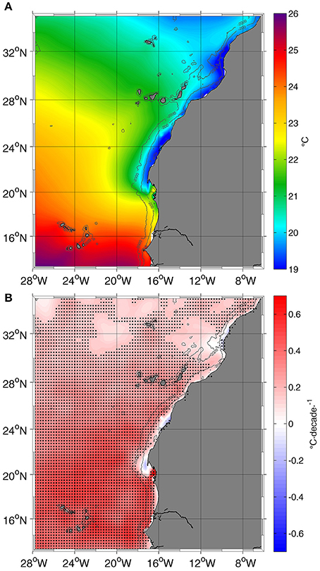
Figure 2. Mean SST (A) and SST trend (B) for the 1993–2014 period. In (B) black dots correspond to significant trends (p < 0.05). 200 and 2,000 m isobaths are represented by gray contour lines.

TABLE 1

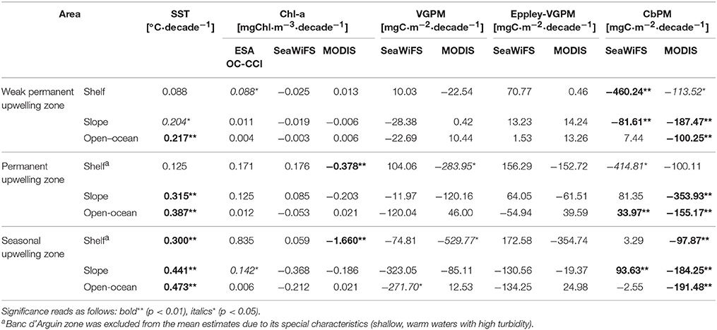
Table 1. Average trends for SST (1993–2014), Chl-a and NPP (VGPM, Eppley-VGPM, and CbPM), for 1998–2007 (SeaWiFS) and 2003–2015 (MODIS) periods in each of the upwelling subregions over the shelf (0–200 m), continental slope (200–2,000 m) and open-ocean region (>2,000 m, as far as 28°W).

Trends in NPP and Chl-a

Computed NPP trends show very different results depending on the model and the dataset (which comprise both the time period and sensor factors). Both the VGPM (Figure 3) and Eppley-VGPM (Figure 4) exhibit similar trends, although these are more marked in the former. For the SeaWiFS dataset two patterns can be clearly identified: an increasing trend over the shelf near Cape Blanc (around 600–800 mgC·m⁻²·decade⁻¹) and a decreasing one around it. Nevertheless, note that only in some patches the trends are significant (p < 0.05). Regarding the two other upwelling subregions, both present zones of slight increase/reduction of NPP. Average trend values for the VGPM over the shelf in the SUZ, PUZ and WPUZ are −75, 105, and 10 mgC·m⁻²·decade⁻¹, respectively, whereas the Eppley-VGPM shows increases of 175, 160, and 70 mgC·m⁻²·decade⁻¹; in neither case are they significant (Table 1). On the other hand, the MODIS datasets are dominated by decreases in NPP (Figures 3, 4). VGPM mean trends over the shelf are −530, −285 and −25 mgC·m⁻²·decade⁻¹ in the SUZ, PUZ and WPUZ, respectively, the first two being significant (p < 0.05). Similarly, the Eppley-VGPM yields non-significant changes in NPP of −355, −155 and 0 mgC·m⁻²·decade⁻¹ for the same zones (Table 1).

FIGURE 3

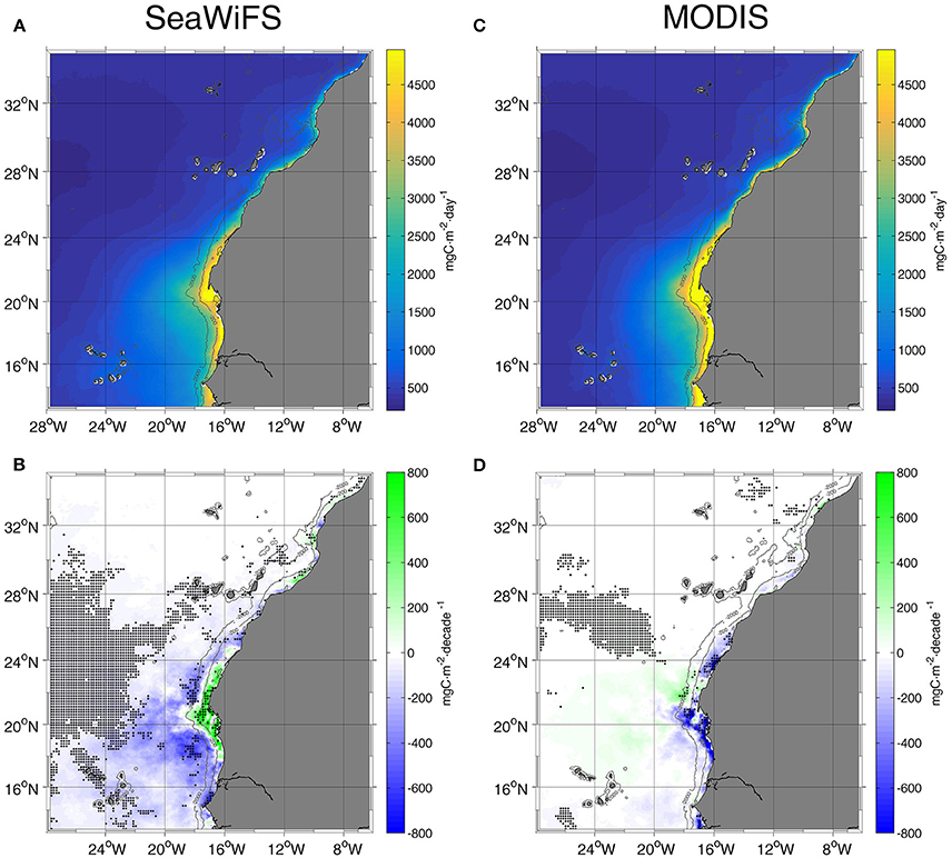
Figure 3. Mean VGPM (A,C) and VGPM trend (B,D) maps for SeaWiFS (1998–2007, left column) and MODIS (2003–2015, right column) datasets. In (B,D), black dots correspond to significant trends (p < 0.05). 200 and 2,000 m isobaths are represented by contour lines.

FIGURE 4

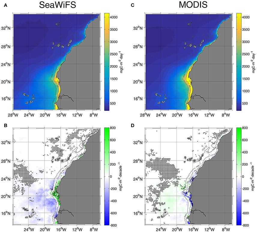
Figure 4. Mean Eppley-VGPM (A,C) and Eppley-VGPM trend (B,D) maps for SeaWiFS (1998–2007, left column) and MODIS (2003–2015, right column) datasets. In (B,D) black dots correspond to significant trends (p < 0.05). 200 and 2000 m isobaths are represented by contour lines.

In general, the CbPM (Figure 5) exhibits different trends relative to the chlorophyll-based VGPM models. The SeaWiFS dataset registers a marked significant decreasing trend exceeding −400 mgC·m⁻²·decade⁻¹ (p < 0.001) over most of the WPUZ and PUZ (Figure 5 and Table 1). On the other hand, the SUZ barely shows any change. Nevertheless, it is worth noting the highly significant (p < 0.001) positive trend off Cape Blanc, with broad areas exceeding 200 mgC·m⁻²·decade⁻¹. The MODIS dataset yields different tendencies: no apparent changes are registered for most of shelf waters over the entire study area (Figure 5). However, mean trends result in significant decreases of −100 and −110 mgC·m⁻²·decade⁻¹ for the SUZ and WPUZ, respectively, and a non-significant drop of −100 mgC·m⁻²·decade⁻¹ for the PUZ (Table 1). Off the continental break, significant declines in NPP are observed widespread (Figure 5).

FIGURE 5

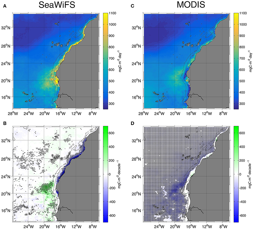
Figure 5. From top to bottom, mean CbPM (A,C) and CbPM trend (B,D) maps for SeaWiFS (1998–2007, left column) and MODIS (2003–2015, right column) datasets. In (B,D) black dots correspond to significant trends (p < 0.05). 200 and 2,000 m isobaths are represented by contour lines.

These results reveal that absolute values and trends in NPP greatly vary depending on the chosen dataset and, especially, model. Absolute NPP mean values show marked differences between Chl-based models and CbPM. In the most productive areas (e.g., Cape Blanc) these discrepancies are magnified, VGPM/Eppley-VGPM showing fourfold NPP values relative to CbPM. Regarding decadal change rates in NPP, a detailed comparison of the average trends in the shelf portion of each of the upwelling zones (Table 1) is shown in Figure 6. For the SeaWiFS dataset, the VGPM and Eppley-VGPM show no significant changes, while the CbPM presents remarkable reductions in the WPUZ and PUZ regions (Table 1). The three models only agree in the SUZ, where NPP estimates do not show any clear trend. Nonetheless, a common feature in the VGPM, Eppley-VGPM and CbPM is the marked seasonality of NPP in all three upwelling zones, reflecting the annual cycle in solar irradiance. On the other hand, for the MODIS dataset all three models agree fairly well in a qualitative sense, exhibiting decreases in all the upwelling zones. Notably, CbPM trends shift from marked decreases in SeaWiFS data to more gentle ones in the MODIS dataset. VGPM and Eppley-VGPM also show changes among SeaWiFS and MODIS datasets, as overall increases are registered in the former and decreases in the latter. When comparing SeaWiFS and MODIS trends in their shared period (2003–2007), both VGPM and Eppley-VGPM show trends that qualitatively match, except in some areas between the Canary Islands and the Cape Verde archipelagos (Supplementary Figure 1), where weak, non-significant trends shift from positive to negative (and viceversa). CbPM trends, on the other hand, exhibit large areas of opposing trends in the open ocean, but agree in the shelf area north of Cape Blanc (21°N). Thus, SeaWiFS and MODIS trends agree reasonably well between 2003 and 2007 for areas close to the upwelling. However, in terms of absolute NPP values it is interesting to notice that SeaWiFS always yields higher values for CbPM than MODIS, whereas the opposite is true for the VGPM and Eppley-VPGM models.

FIGURE 6

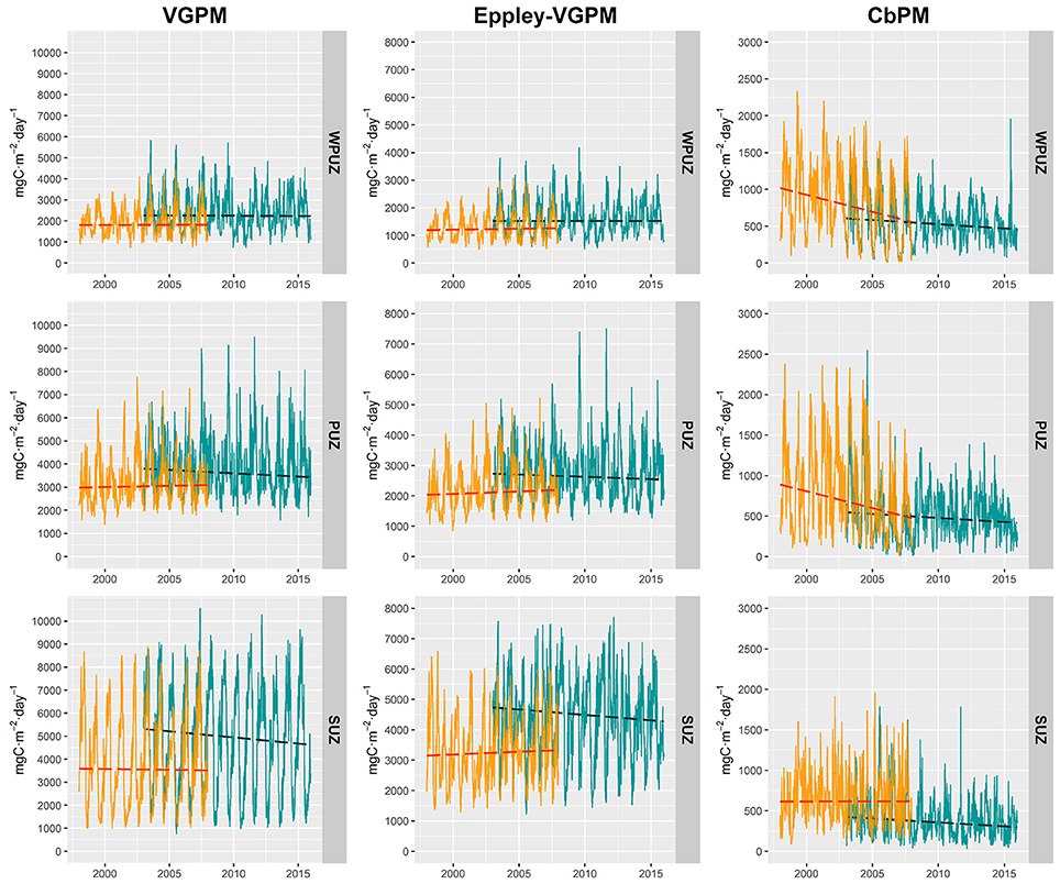
Figure 6. Average time series in the shelf portion of each upwelling zone and their corresponding trend (dashed, Table 1) for VGPM, Eppley-VGPM, CbPM. Orange corresponds to SeaWiFS-based data and blue to MODIS-based data.

Chl-a trends exhibit no significant changes except for some areas north of Cape Ghir (30°N) and around Cap Vert (14°N) (Supplementary Figure 2). This is due to the fact that increases in the first part of the time-series are followed by a stagnant period until ~2010, when the Chl-a starts falling. Average OC-CCI Chl-a trend values over the shelf differ between upwelling zones, being 0.09, 0.17, and 0.83 mg Chl·m⁻³·decade⁻¹ in the WPUZ, PUZ, and SUZ, respectively (Table 1), although only the first one is significant at p < 0.05. However, time-series (Figure 7) seem to show an initial increasing period followed by a decreasing last one. When looking at the individual Chl-a datasets differences are observed between them. SeaWiFS Chl-a shows no significant changes, with trends of 0.06, 0.18 and −0.03 mgChl·m⁻³·decade⁻¹ in the SUZ, PUZ, and WPUZ, respectively (Table 1). On the other hand, for MODIS Chl-a significant negative trends (p < 0.01) of −1.66 and −0.38 mgChl·m⁻³·decade⁻¹ are registered in the SUZ and PUZ, respectively, whereas no significant variation is observed in the WPUZ. Overall, OC-CCI exhibits lower Chl-a concentrations than MODIS and SeaWiFS, although being very close to the latter from 2002 to 2007.

FIGURE 7

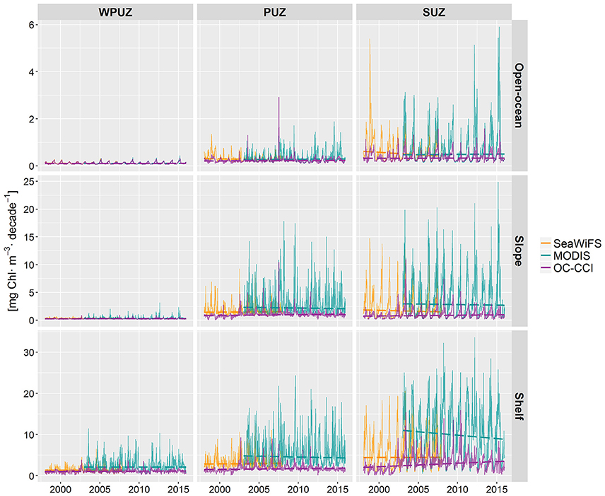
Figure 7. Average Chl-a time-series (light, solid lines) and average trends (dark, dashed lines) for the 1998–2015 period for various datasets in each of the upwelling subregions, over the shelf (0–200 m), continental slope (200–2,000 m) and open-ocean region (>2,000 m, as far as 28°W). Trend values and their significance is shown in Table 1.

Seasonal Climatological Anomalies

The most apparent aspect about seasonal climatological anomalies is that, in general, there is considerable spatial variability between the different upwelling zones studied. SST is, however, the variable which exhibits lower subregional variability (Figure 8). In all the three zones SST anomalies (reaching or exceeding ±0.5°C) follow a similar pattern, with remarkable periods of negative anomalies between 1993–1995 and 1998–2003 (with the exception of 2002), and positive anomalies between 2003–2007 and 2009–2011.

FIGURE 8

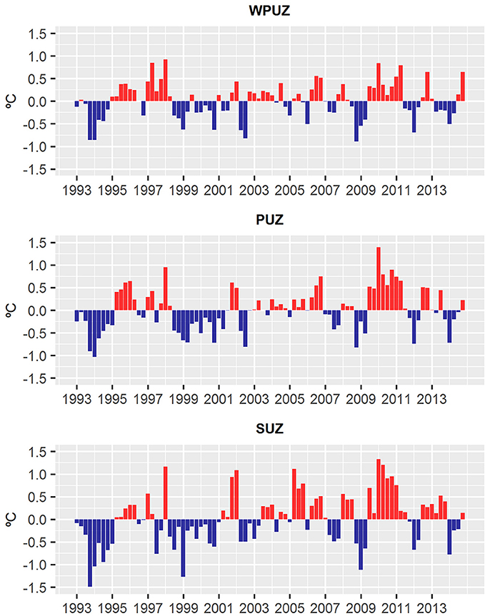
Figure 8. Seasonal SST climatological anomalies in each upwelling zone for the 1993–2014 period.

NPP (Figure 9) and Chl-a anomalies present differences depending on upwelling zone and the production model. Overall, the VGPM and Eppley-VGPM show alternate positive and negative anomalies, whereas the CbPM displays a more regular pattern, especially in the MODIS dataset, where anomalies switch from positive to negative halfway through the 2003–2015 period. Regarding spatial variability, overall anomalies increase southwards, from the WPUZ to the PUZ and SUZ, especially for the VGPM and Eppley-VGPM, evidencing differences in the degree of the changes experienced by each upwelling zone.

FIGURE 9

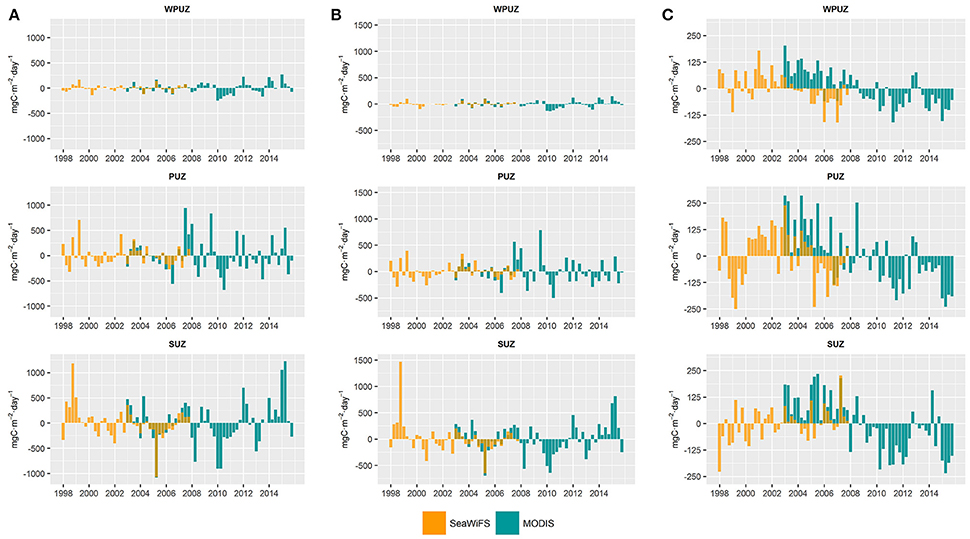
Figure 9. Climatological anomalies of NPP for each upwelling zone. From left to right: VGPM (A), Eppley-VGPM (B) and CbPM (C). Orange corresponds to the SeaWiFS dataset (1998–2007) and blue to the MODIS dataset (2003–2015).

Variability Associated with Climate Modes

The correlation analyses between the ENSO indices and the lagged SST yield no significant results. On the other hand, correlations between SST and various climate indices for the North Atlantic and Pacific Oceans with no lag applied show some significant results (Table 2). Significant negative correlations of SST with the NAO are found widespread (especially with NAO-SB and to a lesser extent with NAO-PC) during winter, spring and autumn, particularly at the PUZ and WPUZ. On the contrary, EA, SOI, and MEI show only sporadic significant correlations with SST.

TABLE 2

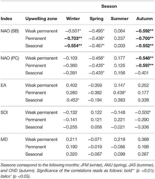
Table 2. Correlations between seasonal SST anomalies and selected climate indices with no lag applied for the 1993–2014 period.

Regarding the NPP models, VGPM and Eppley-VGPM show some high, significant positive correlations with NAO indices when the MODIS dataset is considered, especially during winter (Table 3). This would agree with the SST correlations, as higher temperatures (less upwelling) would be related to lower NPP, and vice versa. CbPM shows only some occasional significant correlations with the climate indices both for SeaWiFS and MODIS datasets.

TABLE 3

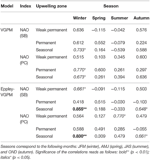
Table 3. Correlations between seasonal selected NPP anomalies and NAO indices (SB, station-based; PC, principal component) with no lag applied for the MODIS dataset (2003–2015).

Discussion

Since Bakun (1990) proposed his upwelling intensification theory more than two decades ago, it has become a matter of increasing interest, especially in the last few years, as growing attention has been paid to global warming and more accurate satellite and model data have become available. Several studies have been published (see references in the following sections) addressing this subject, but it has not been possible to reach a consensus. Different results, both supporting and rejecting Bakun's hypothesis, suggest opposite trends even for the same EBUEs.

Linear Trends

Trends in SST

Computed SST trends reflect a non-surprising overall warming of the ocean, which has been extensively described in the literature over the last years (Levitus et al., 2000, 2005; Hansen et al., 2006, 2010; Domingues et al., 2008; Lyman et al., 2010; Gouretski et al., 2012). Warming trends calculated in the present work for this specific oceanic region are slightly weaker than those found in the literature. Demarcq (2009) used AVHRR pathfinder v5 SST data to estimate trends for the 1998–2007 period. Although the pattern is similar, his average trends were stronger than those obtained in the present work. This might be explained in part by the fact that (1) we used a longer time period for our analysis, (2) he selected different areas for his study, and (3) he used a different method to estimate the trends (Least Absolute Deviations (LAD) instead of the Theil-Sen method employed here). Nevertheless, he did obtain lower warming trends when these were computed for areas with 0–1,000 m depth, i.e., relatively close to the coast, a fact that qualitatively matches the findings presented here. Moreover, in the present work negative trends are registered over the shelf at some locations. This could mean that intensified upwelling of subsurface waters might be occurring, resulting in gentle decreases in SST as a consequence of larger amounts of cool waters reaching the ocean surface. In any case, this would be limited to certain reduced locations (Figure 2B).

McGregor et al. (2007) examined two historical sediment cores (extending back 2,500 years) from Cape Ghir, using the alkenone unsaturation index ($U_{37}^{K^{\prime }}$) as a proxy for SST. For the most part of the twentieth century the sediment cores showed a SST decrease of 1.2°C. Narayan et al. (2010) also studied the Cape Ghir region within the CanC upwelling system as part of their analysis on SST and wind trends in the four major EBUEs. Comparing several wind datasets they obtained contradictory results on meridional wind trends, although the COADS (Comprehensive Ocean Atmosphere Dataset) dataset, the most reliable to their view, exhibited an equatorward wind increase in the CanC. However, caution is required when extrapolating results from Narayan et al. (2010) to the whole CanC EBUE given that the SST upwelling index was estimated exclusively in the northern portion of the WPUZ and meridional wind stress time series correspond to a small region of 3° × 5° of a non-specified location within the upwelling system.

Barton et al. (2013) questioned the results of the abovementioned works. They argued that the use of $U_{37}^{K^{\prime }}$ as a proxy of SST could lead to results biased toward lower SST because of coccolithophores (from which $U_{37}^{K^{\prime }}$ signal is derived) living in deeper layers; i.e., as the ocean warms and stratifies, phytoplankton will tend to occupy deeper parts of the water column and in consequence have less contact with the mixed layer temperatures. Thus, estimating SST from $U_{37}^{K^{\prime }}$ as McGregor et al. (2007) did would bias measures toward lower SSTs than the real ones, as results would truly correspond to cooler subsurface waters. Like Narayan et al. (2010), and Barton et al. (2013) suggested that the evidence for increased upwelling (a greater SST difference between the coast and the open ocean) is not based on a cooling of the coastal waters but on a greater warming of the open ocean waters, as observed in the present work. Furthermore, Barton et al. (2013) analyzed several wind and SST datasets and found that there were not significant changes in meridional wind intensity off NW Africa but a significant SST increase. Consequently, they did not find any strong evidence supporting Bakun's hypothesis.

Cropper et al. (2014) estimated SST trends from HadISST (Hadley Centre Sea Ice and Sea Surface Temperature) and OISST (Optimum Interpolation Sea Surface Temperature) datasets for the summer months (June to August), i.e., when the trade winds are strongest. Their findings showed a very weak negative SST trend for the PUZ, although the trend was not significant even at the 0.1 level. They also found a significant increase in the equatorward meridional wind in several datasets but, once again, the significance limit is set at the 0.1 level, challenging the interpretation of the results.

Trends in NPP and Chl-a

NPP and Chl-a can be used as proxies for upwelling intensity because, although they depend on several factors, upwelling of deep waters is the primary driver of the amount of available nutrients for phytoplankton, which in turn control NPP and Chl-a concentration (Ohde and Siegel, 2010; Messié and Chavez, 2015).

Trends for the times series of the three NPP models present quite different results. Seasonal to decadal changes in the VGPM and Eppley-VGPM are nearly exclusively located around and south of Cape Blanc, and with the exception of some isolated patches they are not statistically significant (Figures 3, 4). Notably, the robustness of the data in the southern subregion of the CanC is affected by the high occurrence of cloud coverage (even on a weekly basis, Supplementary Figure 3), which is particularly persistent during summer months. Furthermore, the PUZ and WPUZ exhibit no significant trends at all. This seems to indicate that no variation in upwelling intensity is experienced for the studied period. On the contrary, the CbPM shows large areas with significant opposite trends (Figure 5). The sharp, significantly negative trends observed with the SeaWiFS dataset in the shelf portion of the PUZ and WPUZ suggest an important decadal decrease in upwelling activity. On the other hand, the MODIS dataset shows very weak trends. Discrepancies in absolute values yielded by the models and datasets also contribute to this conundrum. However, when trends are qualitatively compared for the common SeaWiFS and MODIS period overall they agree reasonably well, with differences only arising where weak, non-significant trends are registered (Supplementary Figure 1). The quantitative shift from lower NPP estimates during the SeaWiFS period to higher ones during the MODIS period observed for VGPM and Eppley-VGPM in shelf areas (Figure 6) is presumably consequence of differences in Chl-a retrievals by these two sensors. Arun Kumar et al. (2015) reported that MODIS overestimated Chl-a relative to SeaWiFS in coastal, eutrophic waters of the Arabian Sea. Demarcq and Benazzouz (2015) found similar results for the CanC region, reporting that MODIS underestimated Chl-a values relative to those estimated by SeaWiFS for low for concentrations (~<0.4 mg·m⁻³) while overestimated Chl-a for high concentrations (~<1 mg·m⁻³). The latter case is relevant when estimating Chl-a concentrations in upwelled waters of the CanC, which largely exceed that value. However, these differences occur consistently and, thus, qualitative comparisons of trends should be acceptable. As outlined by Demarcq and Benazzouz (2015), these discrepancies between SeaWiFS and MODIS estimates arise from differences in (1) calibration and atmospheric correction, (2) correction of sensor sensitivity drifts, and (3) constraints in data processing, e.g., cloud masking, which is of importance particularly in the southern part of the CanC, where cloud coverage is considerable (Supplementary Figure 3). The combination of these issues would also explain the observed differences in NPP, as estimates from the VGPM models are closely related to the Chl-a concentration. Thus, discrepancies between models seem to remain the major issue. In situ primary production (PP) measurements with which to compare model NPP estimates are scarce in the CanC system. Arístegui et al. (2004) compiled available PP data from coastal waters of the CanC upwelling system found in literature, but the bulk of the studies were carried out during the 1970s and 1980s, i.e., before the start of the NPP time-series and thus they cannot be accurately validated. However, model estimates fall between the observed in situ measurements, which ranged between ~1,000–4,000 mg C·m⁻²·day⁻¹, depending on location and season. Yearly mean in situ PP for 31.5–18°N yielded values of 2,400 ± 1,500 mg C·m⁻²·day⁻¹. If compared to mean values from this work (Table 4), Eppley-VGPM is the model that gets closest to in situ measurements, yielding 2,139 ± 610 and 2,731 ± 769 mg C·m⁻²·day⁻¹ for SeaWiFS and MODIS, respectively. On the other hand, VGPM presents higher values (~3,000–3,700 mg C·m⁻²·day⁻¹) whereas CbPM exhibits markedly lower NPP (~500–800 mg C·m⁻²·day⁻¹). This result (VGPM presenting greater NPP values than CbPM) contrasts with the findings of Westberry et al. (2008), who reported the opposite for the global ocean. Their regional results also show greater values for CbPM in gyres and subtropics, whereas VGPM exceeds CbPM estimates in high latitudes. The present work provides evidence that an independent comparison for EBUEs is needed as models show a different behavior to that exhibited in the broad subtropical domains.

TABLE 4

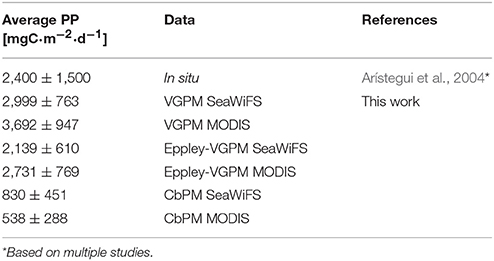
Table 4. In situ PP measurements in coastal waters compared to model NPP estimates over the shelf (0–200 m), for 31.5–18°N.

Kahru et al. (2009) showed that in the California Current region the VGPM adjusted better to in situ NPP measurements (obtained from the large CalCOFI data base) than the CbPM (r² = 0.662 vs. r² = 0.389, respectively), although both models seemed to overestimate NPP. The disagreement between the model outputs, which is also observed in the present work, might arise from dissimilarities in the way the models estimate NPP, as well as in errors from the input data. As mentioned by Kahru et al. (2009), the VGPM (and Eppley-VGPM) requires three input fields while the CbPM needs five (six in the modified version), thus increasing uncertainties in derived NPP. Moreover, the authors argue that the CbPM depends on the GSM algorithm to derive Chl-a and b_bp estimates from water leaving radiance, which is a source of errors especially near the coast (mainly due to colored dissolved organic matter and suspended sediments) and when complex atmospheric conditions are present (Kostadinov et al., 2007). Additional error sources in the CanC upwelling system may arise from the phytoplanktonic community composition and the effect of dust on remote sensing measurements. In parts of the NW African coastal upwelling, where mixotrophy can certainly be a major feature of the planktonic community (Anabalón et al., 2014), Chl-a might not be the most adequate proxy to infer NPP: mixotrophic phytoplankton groups would contribute to increase carbon:Chl-a ratios, thus possibly biasing the output from NPP models based on Chl-a. However, the importance of mixotrophy regarding the entire CanC system remains poorly understood, as very few studies on phytoplanktonic community structure have been carried out. Another potential issue with Chl-a-based NPP estimates is the overestimation of Chl-a concentrations as a consequence of poor atmospheric correction. For instance, Diouf et al. (2013) argued that the SeaWiFS algorithm overestimates aerosol reflectance in the blue and green bands when weakly absorbing aerosols are present, producing lower sea surface reflectances and thus presumably yielding overestimated Chl-a concentrations. Considering the high transport rates of mineral aerosols to the study area from the Saharan desert and the Sahel (Mahowald et al., 2005), this could be a major issue. Hence, considering all the aforementioned potential error sources from input data it is difficult to contrast the performance of the NPP models themselves.

The marked seasonality exhibited by NPP in WPUZ and PUZ initially might not seem to fit with the upwelling patterns described in classical and recent literature. Wooster et al. (1976) and Van Camp et al. (1991) mentioned three similar zones regarding trade wind seasonality: (1) strong, year-round trade winds between 20 and 25°N, where permanent upwelling is present; (2) persistent trade winds during winter south of 20°N, which fade during summer; and (3) persistent trade winds during summer north of 25°N, which fade during winter. Cropper et al. (2014) followed a similar description except for the northernmost section of the upwelling system. North of 26°N they describe the aforementioned weak permanent annual upwelling zone where, despite the fact that a maximum in upwelling intensity is registered during summer months, its occurrence is year-round. Messié and Chavez (2015) concluded that upwelled macronutrients (especially Si) for the most part of the year, as well as light during winter, control NPP in the CanC upwelling system. Light availability patterns in the CanC EBUE roughly follow the same distribution of trade winds (Demarcq and Somoue, 2015). Between 20 and 26°N high light intensity is registered all year long, but out of this latitudinal band light availability decreases. North of 26°N light is reduced due to a more temperate climate, presenting a summer maximum; south of 20°N light is limited during summer months due to the increase in cloud cover consequence of the northward migration of the Intertropical Convergence Zone (ITCZ). Thus, NPP changes could be attributable mainly to the co-variability of trade winds (and, consequently, upwelled nutrients) and light: NPP peaks during summer in the PUZ and WPUZ, coinciding with the maximum of trade wind and light intensity, whereas in the SUZ highest NPP values are registered during late winter and spring, and fade in summer, following the changes in trade winds and light availability.

Demarcq (2009) estimated SeaWiFS Chl-a trends for the same period as the SeaWiFS dataset in our study. He obtained relatively similar trends, with small differences possibly due to the different areas selected for trend averaging and the distinct methods used to calculate the trends (Theil-Sen method against LAD method). In the two cases the overall decreasing trend in Chl-a (and also in NPP derived from the VGPM/Eppley-VGPM in our study) is less pronounced (or even positive) over the shelf. Demarcq (2009) suggested that this might be due to an increase in upwelling intensity or its intrinsic efficiency. However, he did not estimate the significance of trends, which probably were not significant, as in our study (Table 1). Furthermore, the MODIS dataset shows significant decreasing trends in Chl-a over the shelf in the SUZ and PUZ, which contrast with the upwelling intensification hypothesis. The OC-CCI presents positive trends, but these turned out to be non-significant. In fact, trends seem to be somehow biased by a jump in Chl-a concentrations around 2002. Afterwards, Chl-a concentrations seem to stabilize and start to decrease, matching the observed trend in the MODIS dataset. Differences in absolute Chl-a estimates between SeaWiFS/MODIS and OC-CCI are probably consequence of the merging procedure carried out to generate the latter.

In summary, NPP and Chl-a trends exhibit heterogeneous results depending on the dataset, production model and/or upwelling portion analyzed, but overall a pattern of no significant trends or significant decreases can be observed. Considering these results, one might infer either that the CanC has not been experiencing an intensification in upwelling intensity or that, in fact, a reduction is taking place, as suggested by the CbPM model.

Seasonal Climatological Anomalies

The spatial variability of the anomalies between the three upwelling areas provides insights into ecosystem functioning at subregional scales. In general, WPUZ and PUZ exhibit similar patterns whereas SUZ usually differs from the formers. CbPM is a clear example (Figure 9): anomalies in the SUZ are not coupled to those in the WPUZ and PUZ. Indeed, the upwelling regime of the two northern sections of the system is relatively similar and stable throughout the year, in contrast to the highly variable SUZ. These latitudinal differences suggest that the CanC upwelling system might not respond homogeneously to environmental changes, implying that differences in the evolution of the upwelling zones could be expected in the future.

Variability Associated with Climate Modes

The correlation between the different indices and SST is linked to the intensity of trade winds. Stronger trade winds yield greater upwelling intensity which in turn provokes lower SST. Thus, a potential correlation between upwelling intensity and SOI/MEI would be explained by an atmospheric bridge between the Pacific and Atlantic oceans that regulates the upwelling favorable winds, as suggested by Arístegui et al. (2004) and Roy and Reason (2001). Nevertheless, while these studies reported a significant correlation between the Pacific and Atlantic variability after applying a seasonal time-lag, in our study no significant correlations were observed considering or not a time delay.

The observed correlations between the NAO indices and SST in our study are associated with an intensification (reduction) of upwelling favorable winds and, consequently, with a decrease (increase) of SST in the upwelling area, as mentioned by Arístegui et al. (2004) and Cropper et al. (2014). The results of the present work qualitatively agree with the evidence found by Cropper et al. (2014) that found a significant correlation between upwelling intensity and NAO, but not with ENSO. It should be noted, however, that Cropper et al. (2014) defined the upwelling intensity using two upwelling indices: one derived from wind stress (UI^W) and the other inferred from the difference in SST between the coast and the open ocean (UI^SST). They only found a significant correlation between UI^W and NAO, but not with UI^SST. Similarly, Benazzouz et al. (2014) and Narayan et al. (2010) concluded that a significant correlation was absent between UI^SST and NAO. This could mean that, although UI^SST is a qualitatively acceptable index to characterize upwelling intensity (as suggested by Cropper et al., 2014), it lacks the ability to fully describe upwelling variability, perhaps due to its intrinsic simplicity and vulnerability to suffer variations caused by factors unrelated to upwelling (e.g., open ocean warming episodes).

As upwelling intensity is the main driver of Chl-a (e.g., Ohde and Siegel, 2010) it would be expected to find evidence of a positive correlation between NAO and NPP year round. However, only the VGPM and Eppley-VGPM models present significant correlations with NAO at some of the regions, during autumn and winter, giving evidence of the strong subregional variability. This could possibly be due to wind-driven upwelling not fully explaining the NPP in upwelling systems. Renault et al. (2016) argue that although upwelling generated by large-scale winds is the main driver of NPP and remains valid to explain general trends, it does not fully capture interannual variations. They observed that the reduction of winds near the coast and subsequent decrease in upwelling intensity had little impact on NPP. This partial decoupling of NPP from wind-driven upwelling was explained by the authors as a consequence of the effect of winds in alongshore currents and the eddies.

Conclusions

The principal aim of the present work was to analyze interannual trends of NPP at subregional scale in the CanC upwelling region. Estimated SST trends show a widespread warming in the region, with the exception of some restricted areas around Cape Blanc, Dakhla and Cape Ghir, which show significant decreases. On the other hand, OC-CCI Chl-a shows no significant change over the shelf (except in certain areas), apparently due to a marked increase in ~2002 and generalized decreases during the last part of the studied period, a fact confirmed by trend analyses of individual the SeaWiFS and MODIS datasets. Furthermore, NPP trends estimated for the 1998–2007 (SeaWiFS) and 2003–2015 (MODIS) periods show differences between upwelling zones, but overall present either significant decreases or non-significant changes, suggesting that no upwelling intensification is being experienced. Nonetheless, NPP models yield different average results for upwelling zones, as well as different interannual trends, especially for the SeaWiFS dataset. While the CbPM exhibit marked, significant decreases in the shelf region of the WPUZ and PUZ, the VGPM and Eppley-VGPM show non-significant, subtle changes, although disparities are reduced when the MODIS dataset is considered. In sum, this seems to indicate that no intensification of the upwelling is occurring. These discrepancies in NPP estimates probably arise from errors in input variables such as overestimated Chl-a concentrations due to mineral aerosols, which are an important feature of the study area. Modeled NPP and in situ data comparisons carried out in the California Current have shown that the VGPM correlates better with in situ measurements than the CbPM. Here a comparison with historical data seems to indicate that the Eppley-VGPM is the model that best suits in situ PP measurements. However, considering (1) the reduced amount of in situ measurements, (2) the different time periods covered by them and by model NPP estimates, and (3) the errors introduced to NPP estimates by the input variables, discussing the performance of the models themselves is a difficult task. Consequently, a similar comparative analysis with an extended and more recent data of in situ PP is needed for the CanC upwelling region to elucidate which model reproduces better the actual variability in NPP.

The variability associated with climate modes could be of importance to predict future perturbations in the CanC EBUE, as changes in wind patterns related to variations of climate indices seem to regulate upwelling intensity. An individualized study for each season has proved crucial in this regard as distinct responses have been registered depending on the period of the year. The absence of consensus in bibliography, however, does not allow drawing definitive conclusions, being necessary further studies.

Finally, the results from the present work need to be interpreted with caution, since extrapolating to longer periods can be misleading. Although long SST time series are relatively common, this is not the case for variables such as satellite-derived NPP. Further improvements on NPP models and approaches to combine different Chl-a/NPP datasets, along with recent, more accurate data, will help to build climate data records of satellite-derived biological parameters, eventually allowing for a better comprehension of the evolution of upwelling ecosystems at regional and subregional scales under a climate warming scenario.

Author Contributions

MG-L carried out the analysis of the data, made the figures, and wrote the manuscript. JA acted as an advisor during the development of the study, and contributed to the discussion and the writing of the manuscript. AR acted as an advisor during the development of the study, and contributed to the discussion and the writing of the manuscript. JC participated in the analyses of the data and reviewed the manuscript.

Funding

This is a contribution to the FLUXES project (CTM2015-69392-C3-1-R; Coordinator: JA) funded by the Spanish government (Plan Nacional I+D).

Conflict of Interest Statement

The authors declare that the research was conducted in the absence of any commercial or financial relationships that could be construed as a potential conflict of interest.

Acknowledgments

We would like to thank the data providers mentioned in the Methods section for freely providing the datasets employed in the present work.

Supplementary Material

The Supplementary Material for this article can be found online at: https://www.frontiersin.org/articles/10.3389/fmars.2017.00370/full#supplementary-material

Supplementary Figure 1. Trend agreement between SeaWiFS- and MODIS-based NPP estimates for their common period (2003–2007). If both SeaWiFS- and MODIS-based estimates yield either positive or negative trends, agree. If they yield opposed trends, differ.

Supplementary Figure 2. OC-CCI Chl-a trends for the 1998–2015 period. Black dots correspond to significant trends (p < 0.05). 200 and 2,000 m isobaths are represented by contour lines. See Supplementary Figure 3 for the number of valid observations of each pixel employed in trend estimates.

Supplementary Figure 3. Number of valid observations (out of a total of 828) in the OC-CCI Chl-a dataset. Absence of data is due to cloud cover.

References

Aalst, M., Van Adger, N., Arent, D., Barnett, J., Betts, R., Bilir, E., et al. (2014). Climate Change 2014: impacts, adaptation, and vulnerability. Assess. Rep. 5, 1–76. doi: 10.1017/CBO9781107415379

CrossRef Full Text | Google Scholar

Anabalón, V., Arístegui, J., Morales, C. E., Andrade, I., Benavides, M., Correa-Ramírez, M. A., et al. (2014). The structure of planktonic communities under variable coastal upwelling conditions off Cape Ghir (31°N) in the Canary Current System (NW Africa). Prog. Oceanogr. 120, 320–339. doi: 10.1016/j.pocean.2013.10.015

CrossRef Full Text | Google Scholar

Arístegui, J., Álvarez-Salgado, X. A., Barton, E. D., Figueiras, F. G., Hernández-León, S., Roy, C., et al. (2004). “Oceanography and fisheries of the Canary current/Iberian region of the eastern North Atlantic (18a,E),” in The Sea, eds A. R. Robinson and K. H. Brink (Harvard, MA: Harvard University Press), 877–932.

Google Scholar

Arístegui, J., Barton, E. D., Álvarez-Salgado, X. A., Santos, A. M. P., Figueiras, F. G., Kifani, S., et al. (2009). Sub-regional ecosystem variability in the Canary Current upwelling. Prog. Oceanogr. 83, 33–48. doi: 10.1016/j.pocean.2009.07.031

CrossRef Full Text

Arun Kumar, S. V. V., Babu, K. N., and Shukla, A. K. (2015). Comparative Analysis of Chlorophyll- a Distribution from SeaWiFS, MODIS-Aqua, MODIS-Terra and MERIS in the Arabian Sea. Mar. Geod. 38, 40–57. doi: 10.1080/01490419.2014.914990

CrossRef Full Text | Google Scholar

Bakun, A. (1990). Global climate change and intensification of coastal ocean upwelling. Science 247, 198–201. doi: 10.1126/science.247.4939.198

PubMed Abstract | CrossRef Full Text | Google Scholar

Banse, K. (1991). Rates of phytoplankton cell division in the field and in iron enrichment experiments. Limnol. Oceanogr. 36, 1886–1898. doi: 10.4319/lo.1991.36.8.1886

CrossRef Full Text | Google Scholar

Barton, E. D., Field, D. B., and Roy, C. (2013). Canary current upwelling: more or less? Prog. Oceanogr. 116, 167–178. doi: 10.1016/j.pocean.2013.07.007

CrossRef Full Text | Google Scholar

Behrenfeld, M. J., and Falkowski, P. G. (1997). Photosynthetic rates derived from satellite-based chlorophyll concentration. Limnol. Oceanogr. 42, 1–20. doi: 10.4319/lo.1997.42.1.0001

CrossRef Full Text | Google Scholar

Behrenfeld, M. J., Boss, E., Siegel, D. A., and Shea, D. M. (2005). Carbon-based ocean productivity and phytoplankton physiology from space. Global Biogeochem. Cycles 19, 1–14. doi: 10.1029/2004GB002299

CrossRef Full Text | Google Scholar

Behrenfeld, M. J., O'Malley, R. T., Siegel, D. A., McClain, C. R., Sarmiento, J. L., Feldman, G. C., et al. (2006). Climate-driven trends in contemporary ocean productivity. Nature 444, 752–755. doi: 10.1038/nature05317

PubMed Abstract | CrossRef Full Text | Google Scholar

Belkin, I. M. (2009). Rapid warming of large marine ecosystems. Prog. Oceanogr. 81, 207–213. doi: 10.1016/j.pocean.2009.04.011

CrossRef Full Text | Google Scholar

Benazzouz, A., Mordane, S., Orbi, A., Chagdali, M., Hilmi, K., Atillah, A., et al. (2014). An improved coastal upwelling index from sea surface temperature using satellite-based approach - The case of the Canary Current upwelling system. Cont. Shelf Res. 81, 38–54. doi: 10.1016/j.csr.2014.03.012

CrossRef Full Text | Google Scholar

Boyce, D. G., Lewis, M. R., and Worm, B. (2010). Global phytoplankton decline over the past century. Nature 466, 591–596. doi: 10.1038/nature09268

PubMed Abstract | CrossRef Full Text | Google Scholar

Carr, M. E., and Kearns, E. J. (2003). Production regimes in four Eastern Boundary Current systems. Deep. Res. Part II Top. Stud. Oceanogr. 50, 3199–3221. doi: 10.1016/j.dsr2.2003.07.015

CrossRef Full Text | Google Scholar

Chavez, F. P., and Messié, M. (2009). A comparison of Eastern boundary upwelling ecosystems. Prog. Oceanogr. 83, 80–96. doi: 10.1016/j.pocean.2009.07.032

CrossRef Full Text | Google Scholar

Chavez, F. P., Messié, M., and Pennington, J. T. (2011). Marine primary production in relation to climate variability and change. Ann. Rev. Mar. Sci. 3, 227–260. doi: 10.1146/annurev.marine.010908.163917

PubMed Abstract | CrossRef Full Text | Google Scholar

Cropper, T. E., Hanna, E., and Bigg, G. R. (2014). Spatial and temporal seasonal trends in coastal upwelling off Northwest Africa, 1981-2012. Deep. Res. Part I Oceanogr. Res. Pap. 86, 94–111. doi: 10.1016/j.dsr.2014.01.007

CrossRef Full Text | Google Scholar

Demarcq, H. (2009). Trends in primary production, sea surface temperature and wind in upwelling systems (1998-2007). Prog. Oceanogr. 83, 376–385. doi: 10.1016/j.pocean.2009.07.022

CrossRef Full Text | Google Scholar

Demarcq, H., and Benazzouz, A. (2015). “Trends in phytoplankton and primary productivity off Northwest Africa,” in Oceanographic and Biological Features in the Canary Current Large Marine Ecosystem, eds L. Valdés and I. Déniz-González (Paris: IOC-UNESCO), 331–341. Available online at: http://hdl.handle.net/1834/9199

Google Scholar

Demarcq, H., and Somoue, L. (2015). “Phytoplankton and primary productivity off Northwest Africa,” in Oceanographic and biological features in the Canary Current Large Marine Ecosystem, eds L. Valdés and I. Déniz-González (Paris: IOC-UNESCO), 161–174. Available Online at: http://hdl.handle.net/1834/9186

Google Scholar

Diouf, D., Niang, A., Brajard, J., Crepon, M., and Thiria, S. (2013). Retrieving aerosol characteristics and sea-surface chlorophyll from satellite ocean color multi-spectral sensors using a neural-variational method. Remote Sens. Environ. 130, 74–86. doi: 10.1016/j.rse.2012.11.002

CrossRef Full Text | Google Scholar

Domingues, C. M., Church, J. A., White, N. J., Gleckler, P. J., Wijffels, S. E., Barker, P. M., et al. (2008). Improved estimates of upper-ocean warming and multi-decadal sea-level rise. Nature 453, 1090–1093. doi: 10.1038/nature07080

PubMed Abstract | CrossRef Full Text | Google Scholar

Eppley, R. W. (1972). Temperature and phytoplankton growth in the sea. Fish. Bull. 70, 1063–1085.

Google Scholar

Gille, S. T. (2002). Warming of the Southern Ocean since the 1950s. Science 295, 1275–1277. doi: 10.1126/science.1065863

PubMed Abstract | CrossRef Full Text | Google Scholar

Gouretski, V., Kennedy, J., Boyer, T., and Khl, A. (2012). Consistent near-surface ocean warming since 1900 in two largely independent observing networks. Geophys. Res. Lett. 39:L19606. doi: 10.1029/2012GL052975

CrossRef Full Text | Google Scholar

Hamed, K. H., and Ramachandra Rao, A. (1998). A modified Mann-Kendall trend test for autocorrelated data. J. Hydrol. 204, 182–196. doi: 10.1016/S0022-1694(97)00125-X

CrossRef Full Text | Google Scholar

Hansen, J., Ruedy, R., Sato, M., and Lo, K. (2010). Global surface temperature change. Rev. Geophys. 48:RG4004. doi: 10.1029/2010RG000345

CrossRef Full Text | Google Scholar

Hansen, J., Sato, M., Ruedy, R., Lo, K., Lea, D. W., and Medina-Elizade, M. (2006). Global temperature change. Proc. Natl. Acad. Sci. U.S.A. 103, 14288–14293. doi: 10.1073/pnas.0606291103

PubMed Abstract | CrossRef Full Text | Google Scholar

Ihara, C., Kushnir, Y., and Cane, M. A. (2008). Warming trend of the Indian Ocean SST and Indian Ocean dipole from 1880 to 2004. J. Clim. 21, 2035–2046. doi: 10.1175/2007JCLI1945.1

CrossRef Full Text | Google Scholar

Kahru, M., Kudela, R., Manzano-Sarabia, M., and Mitchell, B. G. (2009). Trends in primary production in the California Current detected with satellite data. J. Geophys. Res. Ocean. 114:C02004. doi: 10.1029/2008JC004979

CrossRef Full Text | Google Scholar

Kostadinov, T. S., Siegel, D. A., Maritorena, S., and Guillocheau, N. (2007). Ocean color observations and modeling for an optically complex site: Santa Barbara Channel, California, U. S. A. J. Geophys. Res. Ocean. 112, 1–15. doi: 10.1029/2006JC003526

CrossRef Full Text | Google Scholar

Levitus, S., Antonov, J. I., Boyer, T. P., and Stephens, C. (2000). Warming of the world ocean. Science 287, 2225–2229. doi: 10.1126/science.287.5461.2225

CrossRef Full Text | Google Scholar

Levitus, S., Antonov, J., and Boyer, T. (2005). Warming of the world ocean, 1955-2003. Geophys. Res. Lett. 32:L02604. doi: 10.1029/2004GL021592

CrossRef Full Text | Google Scholar

Lyman, J. M., Good, S. A., Gouretski, V. V., Ishii, M., Johnson, G. C., Palmer, M. D., et al. (2010). Robust warming of the global upper ocean. Nature 465, 334–337. doi: 10.1038/nature09043

PubMed Abstract | CrossRef Full Text | Google Scholar

Mahowald, N. M., Baker, A. R., Bergametti, G., Brooks, N., Duce, R. A., Jickells, T. D., et al. (2005). Atmospheric global dust cycle and iron inputs to the ocean. Global Biogeochem. Cycles 19:GB4025. doi: 10.1029/2004GB002402

CrossRef Full Text | Google Scholar

Martinez, E., Antoine, D., D'Ortenzio, F., Gentili, B., Antoine, D., Morel, A., et al. (2009). Climate-driven basin-scale decadal oscillations of oceanic phytoplankton. Science 326, 1253–1256. doi: 10.1126/science.1177012

PubMed Abstract | CrossRef Full Text | Google Scholar

McGregor, H. V., Dima, M., Fischer, H. W., and Mulitza, S. (2007). Rapid 20th-century increase in coastal upwelling off northwest Africa. Science 315, 637–639. doi: 10.1126/science.1134839

PubMed Abstract | CrossRef Full Text | Google Scholar

Messié, M., and Chavez, F. P. (2015). Seasonal regulation of primary production in eastern boundary upwelling systems. Prog. Oceanogr. 134, 1–18. doi: 10.1016/j.pocean.2014.10.011

CrossRef Full Text | Google Scholar

Morel, A. (1991). Light and marine photosynthesis: a spectral model with geochemical and climatological implications. Prog. Oceanogr. 26, 263–306. doi: 10.1016/0079-6611(91)90004-6

CrossRef Full Text | Google Scholar

Narayan, N., Paul, A., Mulitza, S., and Schulz, M. (2010). Trends in coastal upwelling intensity during the late 20th century. Ocean Sci. 6, 815–823. doi: 10.5194/os-6-815-2010

CrossRef Full Text | Google Scholar

Nieves, V., Willis, J. K., and Patzert, W. C. (2015). Recent hiatus caused by decadal shift in Indo-Pacific heating. Science 349, 532–535. doi: 10.1126/science.aaa4521

PubMed Abstract | CrossRef Full Text | Google Scholar

Oerder, V., Colas, F., Echevin, V., Codron, F., Tam, J., and Belmadani, A. (2015). Peru-Chile upwelling dynamics under climate change. J. Geophys. Res. C Ocean. 120, 1152–1172. doi: 10.1002/2014JC010299

CrossRef Full Text | Google Scholar

Ohde, T., and Siegel, H. (2010). Biological response to coastal upwelling and dust deposition in the area off Northwest Africa. Cont. Shelf Res. 30, 1108–1119. doi: 10.1016/j.csr.2010.02.016

CrossRef Full Text | Google Scholar

Renault, L., Deutsch, C., McWilliams, J. C., Frenzel, H., Liang, J.-H., and Colas, F. (2016). Partial decoupling of primary productivity from upwelling in the California Current system. Nat. Geosci. 9, 505–508. doi: 10.1038/ngeo2722

CrossRef Full Text | Google Scholar

Roy, C., and Reason, C. (2001). ENSO related modulation of coastal upwelling in the eastern Atlantic. Prog. Oceanogr. 49, 245–255. doi: 10.1016/S0079-6611(01)00025-8

CrossRef Full Text | Google Scholar

Sangrà, P., Pascual, A., Rodríguez-Santana, Á., Machín, F., Mason, E., McWilliams, J. C., et al. (2009). The canary eddy Corridor: a major pathway for long-lived eddies in the subtropical North Atlantic. Deep. Res. Part I Oceanogr. Res. Pap. 56, 2100–2114. doi: 10.1016/j.dsr.2009.08.008

CrossRef Full Text | Google Scholar

Sen, P. K. (1968). Estimates of the regression coefficient based on Kendall's Tau. J. Am. Stat. Assoc. 63, 1379–1389. doi: 10.1080/01621459.1968.10480934

CrossRef Full Text | Google Scholar

Smith, W. H., and Sandwell, D. (1997). Global Sea Floor Topography from Satellite Altimetry and Ship Depth Soundings. Science 277, 1956–1962. doi: 10.1126/science.277.5334.1956

CrossRef Full Text | Google Scholar

Snyder, M. A., Sloan, L. C., Diffenbaugh, N. S., and Bell, J. L. (2003). Future climate change and upwelling in the California Current. Geophys. Res. Lett. 30:1823. doi: 10.1029/2003GL017647

CrossRef Full Text | Google Scholar

Sydeman, W. J., García-Reyes, M., Schoeman, D. S., Rykaczewski, R. R., Thompson, S. A., Black, B. A., et al. (2014). Climate change and wind intensification in coastal upwelling ecosystems. Science 345, 77–80. doi: 10.1126/science.1251635

PubMed Abstract | CrossRef Full Text | Google Scholar

Theil, H. (1950). A rank-invariant method of linear and polynomial regression analysis. I. Nederl. Akad. Wetensch. Proc. 53, 386–392.

Van Camp, L., Nykjaer, L., Mittelstaedt, E., and Schlittenhardt, P. (1991). Upwelling and boundary circulation off Northwest Africa as depicted by infrared and visible satellite observations. Prog. Oceanogr. 26, 357–402. doi: 10.1016/0079-6611(91)90012-B

CrossRef Full Text | Google Scholar

Varela, R., Álvarez, I., Santos, F., DeCastro, M., and Gómez-Gesteira, M. (2015). Has upwelling strengthened along worldwide coasts over 1982-2010? Sci. Rep. 5:15. doi: 10.1038/srep10016

PubMed Abstract | CrossRef Full Text | Google Scholar

Wang, D., Gouhier, T. C., Menge, B. A., and Ganguly, A. R. (2015). Intensification and spatial homogenization of coastal upwelling under climate change. Nature 518, 390–394. doi: 10.1038/nature14235

PubMed Abstract | CrossRef Full Text | Google Scholar

Westberry, T., Behrenfeld, M. J., Siegel, D. A., and Boss, E. (2008). Carbon-based primary productivity modeling with vertically resolved photoacclimation. Global Biogeochem. Cycles 22:GB2024. doi: 10.1029/2007GB003078

CrossRef Full Text | Google Scholar

Wooster, W. S., Bakun, A., and McClain, D. R. (1976). The seasonal upwelling cycle along the eastern boundary of the North Atlantic. J. Mar. Res. 34, 131–141.

Google Scholar