A Framework for Combining Seasonal Forecasts and Climate Projections to Aid Risk Management for Fisheries and Aquaculture

Introduction

Marine industries such as fisheries and aquaculture have historically coped with interannual and seasonal environmental variability that affects the presence, growth, and survival of many species (Callaway et al., 2012; Hobday et al., 2016; Salinger et al., 2016). Optimal conditions for catching and farming fish are not always present at the desired time and location (Callaway et al., 2012; Bell et al., 2013; Brander, 2013), which has required development of skills and approaches to cope with environmental variability. For example, interannual changes in species distribution in response to climate drivers such as ENSO have required fishers to temporarily move to new grounds to access fish (e.g., Lehodey et al., 2006), or to delay aquaculture activities in that season (Spillman et al., 2015). However, under long-term climate change, new conditions will be encountered, and past experience may no longer be as useful in managing businesses (Hobday et al., 2016). Thus, new approaches to cope with future environmental conditions may be needed.

Information about future environmental conditions can be used to manage risk in environmentally-exposed industries (Chang et al., 2013; Little et al., 2015). Seasonal forecasting applications in Australia and elsewhere have been developed for a range of marine resource segments, including salmon and prawn aquaculture (Spillman and Hobday, 2014; Spillman et al., 2015), commercial tuna (Hobday et al., 2011; Eveson et al., 2015) and sardine fisheries (Kaplan et al., 2016), and recreational fisheries (Brodie et al., 2017). Depending on the application, these forecasting applications have delivered information on both environmental conditions, such as water temperature, rainfall, and air temperature, and habitat distribution, at lead times of up to 3 months (Hobday et al., 2016), helping managers and fishers to plan activities based on predicted conditions (Eveson et al., 2015; Spillman et al., 2015). These marine industries are thus in a position to make improved management decisions and perform better than those without information about the future environment.

In contrast, longer-term projections of environmental change that will impact the distribution and abundance of marine species, such as tuna (Hobday, 2010; Lehodey et al., 2010; Hartog et al., 2011; Dell et al., 2015; Robinson et al., 2015), have not been as useful to seafood businesses. While policy and management discussions can be informed by projections at long time scales (Bell et al., 2013; Brander, 2013), there are few operational business decisions made at time scales matching climate scale projections. Thus, while many highly cited papers describe changes in marine species distribution and abundance for the year 2100 (e.g., Cheung et al., 2010; Hobday, 2010; Lehodey et al., 2010), the timescale of these studies is less relevant for marine industries currently facing challenging environmental conditions (Spillman and Hobday, 2014). The goal of this paper is to propose one approach to help these industries manage climate variability in the short-term and adapt to climate change in the long-term.

Some marine industries are spatially restricted, including most ocean-based aquaculture businesses largely due to infrastructure associated with holding the farmed species, and so are particularly vulnerable to changing environmental conditions (e.g., Callaway et al., 2012). Likewise, coastal fisheries may have a restricted operating range from a port due to the vessel size, fishing technique, management restrictions, or product shipping requirements (e.g. access to road or air freight). Here we introduce a conceptual framework to help climate-proof these marine industries by using a combination of climate and seasonal forecasting that recognizes the influence of both long-term trends and short-term environmental variability. In this regard, we define climate-proofing as the development of strategies that can equip businesses with skills or information to manage or reduce the risk from climate change. This approach builds on recent development and application of seasonal forecasting tools, which represent one risk-based approach used by the marine resource sector to manage future uncertainty (Battaglene et al., 2008; Hobday et al., 2016; Payne et al., 2017).

We illustrate this framework using long-term climate projections and seasonal forecast examples from southern Australia, where marine-based industries are worth more than A$10B per annum (Bennett et al., 2016). Economically important aquaculture industries worth close to A$1B per annum include salmon, tuna, abalone, oyster, and mussel and are all exposed to environmental change (Savage and Hobsbawn, 2015). This region is experiencing rapid change in terms of ocean warming (Hobday and Pecl, 2014) as well as in the number of extreme events such as marine heatwaves (Oliver et al., 2017), both of which are projected to continue (Oliver et al., 2014). Thus, there is growing interest in forecasting applications to help marine industries in this region (Hobday et al., 2016). Here we focus on forecasts of sea surface temperature (SST), a primary environmental variable that is changing and is influential on aquaculture production via direct impacts on growth and survival and indirect impacts through disease, pests, and equipment fouling (Hobday et al., 2016), and on fisheries through changes in distribution and abundance of the target species (e.g., Madin et al., 2012; Frusher et al., 2016).

The Approach to Climate-Proofing

To understand the potential environmental conditions at seasonal and long-term time scales, information from seasonal-scale and climate-scale models, respectively, is needed. We first provide a brief description of a seasonal-scale and climate-scale model used in Australia, with a focus on SST, whilst noting that each model provides a range of other projected variables that may be useful for different situations and species. We then describe a novel framework that uses information from these two forecasting time scales to support decision makers seeking to manage risk under both climate variability and change.

To generate illustrative long-term projections, we use output from the CSIRO Ocean Downscaling Project (hereafter CSIRO-Downscaling). A global high-resolution (0.1°) ocean general circulation model (OGCM) is used to dynamically downscale climate changes in the twenty-first century derived from Coupled Model Intercomparison Project Phase 5 (CMIP5) climate models (Taylor et al., 2012). The OGCM is the Ocean Forecasting Australia Model Version 3 (OFAM3, Oke et al., 2013), based on version 4p1d of the GFDL Modular Ocean Model (Griffies, 2009), which is configured to have 0.1° grid spacing for all longitudes between 75°S and 75°N, and 51 vertical layers. The global OGCM is integrated over the historical period (1979–2014) driven by 3-h Japanese 55-year Reanalysis (JRA-55, Kobayashi et al., 2015) through bulk formula. Details about model set-up of this historical experiment and validation with observations are provided in Zhang et al. (2016). The model is further integrated from 2006 to 2101, driven by merged atmospheric forcings which include a high-frequency (daily to interannual) part from current-day JRA-55 reanalysis and a long-term climate change part from the ensemble of 17 CMIP5 models under a high emission scenario (RCP8.5) (Zhang et al., 2017). High-resolution (0.1°) model results provide downscaled climate change projections in the twenty-first century for all common ocean state variables including sea level, temperature, and currents.

Example seasonal forecasts are derived here using the new ACCESS-S1 (the seasonal prediction version of the Australian Community Climate and Earth-System Simulator; version 1) seasonal prediction system, developed by the Australian Bureau of Meteorology in collaboration with the UK Met Office (UKMO), CSIRO and universities. ACCESS-S1 is a coupled ocean-atmosphere prediction system comprising the UKMO coupled model GC2, which consists of the latest UKMO atmospheric model, European ocean model NEMO (Nucleus for European Modeling of the Ocean) and sea-ice model CICE (Los Alamos sea ice model), together with land surface model JULES (Joint UK Land Environment Simulator; Lim et al., 2016; Hudson et al., 2017). ACCESS-S1 has considerable enhancements compared to its operational predecessor POAMA-2 (Spillman and Hobday, 2014), including higher ocean grid resolution of 25 km compared to 100–200 km. This marked increase in resolution means that impacts of local weather and climate of narrow features of coastal currents such as the East Australian Current could be resolved and may provide new opportunities for coastal forecasting applications. Example SST forecast skill as a measure of predictive performance for this seasonal model is illustrated here.

Both climate- and seasonal-scale information can be used to manage future environmental risk (Figure 1). Climate projections can help to assess regional suitability from the present time to many decades into the future. For example, given a desired SST range for a farmed or fished species, climate models can give an indication as to if and when SST in a particular region will become unsuitable. If environmental conditions in the region are suitable now and remain so in future, then managing for climate variability with accurate seasonal forecasts will suffice. However if the current region is not suitable now, or will become unsuitable in future, it may be necessary to relocate to a new region based on climate projections, or develop other adaptation strategies (e.g., develop a genetically-adapted lineage if sufficient time exists until the site becomes unsuitable; investigate ways to modify the environment to make it suitable; switch to farming/catching a different species).

FIGURE 1

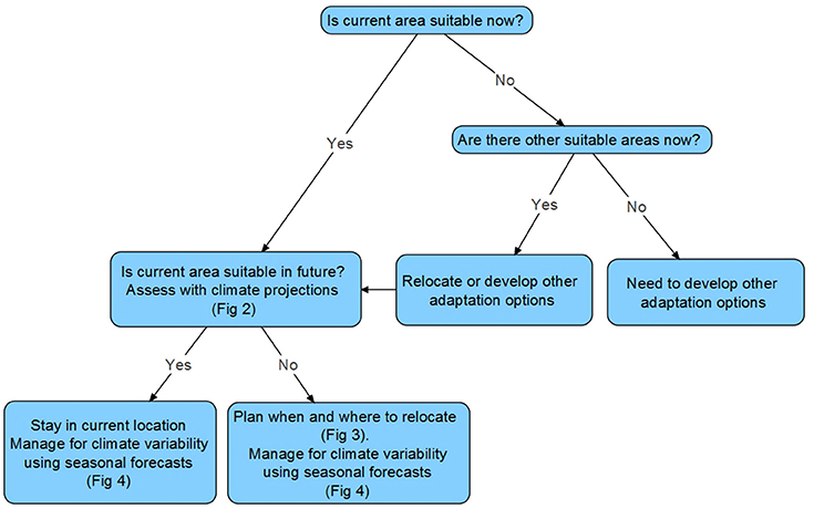
Figure 1. Decision tree to guide climate-proofing approach by aquaculture businesses. Figure numbers refer to subsequent figures.

In southern Australia, SST is projected to warm rapidly over the next 60-80 years, particularly in south-east Australia (Figure 2), which is consistent with climate projections reported in previous studies (Hobday and Lough, 2011; Hobday and Pecl, 2014; Popova et al., 2016). These climate projections indicate that seafood industries across southern Australia will need to consider climate-proofing strategies. For example, eastern Tasmania is already warming rapidly (Hobday and Pecl, 2014), with warming projected to continue (Figure 2; Popova et al., 2016). The upper limit of a representative temperature (e.g., 13–18°C, representing typical maximum summer and winter temperatures) for an indicative species fished or farmed in this region is currently regularly exceeded in north-east Tasmania (Zone 4, Figure 3). To compare between regions, we use as a measure “time of exceedance,” analogous to “time of emergence” used in climate studies (Hawkins and Sutton, 2012; Lyu et al., 2014). While summer temperatures receive attention, cooler temperatures in winter are important for recruitment of some wild species, and can also prevent disease persisting year round in cultured species, thus warmer winters may bring challenges, just as do warm summers. For regions to the south, climate projections indicate the year of first exceedance of unsuitable summer (winter) conditions increases from north (Zone 3) to south (Zone 1): 2018 (2010), 2024 (2030), and 2037 (2032), respectively (Figure 3—middle column). In each region, even as the average SST for a month exceeds a threshold, there will still be areas that may be cooler (Figure 3—right two columns). The time of permanent exceedance (all subsequent summers above the threshold) is 30–45 years later than the year of first exceedance for the summer threshold, and 14–30 years later for the winter threshold, depending on location (Figure 3). If the particular aquaculture or fishing operation needs to have both summer and winter temperatures below these example thresholds, then the time period of suitable conditions is abbreviated. These results should be considered indicative, as they are the results from a single model run with no estimate of uncertainty (Stock et al., 2011), but they illustrate how the time between first and permanent exceedance represents a window in which to use seasonal forecasting, whilst developing a solution for when conditions become permanently unsuitable (Figure 1).

FIGURE 2

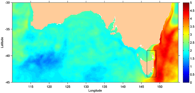
Figure 2. Projected SST change over the period 2081-2100 relative to 1986-2005 for southern Australia based on output from the CSIRO-Downscaling project described in the text. Box shows the area considered in Figure 3.

FIGURE 3

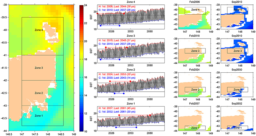
Figure 3. First column: Model sea surface temperature (SST) in eastern Tasmania for February 2016. Middle column: Monthly SST time series for the period 2006-2101 (black line) for the four zones with example warm (18°C) and cold thresholds (13°C) in horizontal black lines, corresponding to maximum tolerances for a hypothetical species in summer and winter, and the average SST for February (Austral summer, red line) and September (Austral winter, blue line), typically the warmest and coldest month respectively. The first and permanent exceedance times for the summer (red dots) and winter (blue dots) are shown for each zone, and provided on each panel (red and blue text), along with the period between first and permanent exceedance. Final two columns: February and September SST maps for the year of first exceedance, showing that in each region, there are pixels where SST is below the threshold values for summer and winter (shaded). Color scale is the same in all maps. Data are from modeling experiments run by the CSIRO-downscaling project.

Future sites can be assessed by considering their suitability under future conditions. For example, as the most northern region (Zone 4) warms, suitable locations based on SST conditions can be found to the south (Figure 3). Thus, in 2048, when the average conditions become permanently unsuitable (outside the range 13–18°C) in Zone 3, there are still some locations within Zone 3 that are suitable, and there are more areas with suitable conditions further to the south. If only a small southward relocation distance is selected by a fishing or aquaculture business, it will likely be necessary to relocate again in future, while a move too far south may be premature for best conditions.

Benefit of Seasonal Forecasting as the Climate Changes

Seasonal forecasts can be used to manage risk due to environmental variability both when the current location is expected to remain suitable in future and when it is expected to become unsuitable (Figure 1). In the first case the main objective is to use short-term forecasts to improve efficiency and increase profits, while in the second case the aim is more to minimize costs and increase the time period over which the current region remains viable for the fishing or farming activity while developing long-term adaptation options.

Specifically, in areas where the environmental suitability for the focal species is good, profits are high relative to costs (Figure 4). If conditions are always suitable (e.g., always between the upper and lower SST threshold), the benefits from seasonal forecasting might not be significant. However, if environmental variability sometimes exceeds the suitable range, even if there is no long-term trend, seasonal forecasts will be beneficial. If the environmental suitability at a location is predicted to decline over time under climate change, operational costs are expected to increase and profits decrease, until business would not be viable. Seasonal forecasts can provide information on upcoming environmental conditions so individual businesses have increased potential to reduce costs and increase profits, relative to no forecast (Hobday et al., 2016). This can allow these businesses to implement proactive response options to remain viable during periods when less suitable environmental conditions occur, even if there is no significant climate change trend (e.g., Spillman and Hobday, 2014; Spillman et al., 2015). Depending on the business, these options might include modifying the environment, changing the fishing or harvesting schedule, increasing or decreasing the production volume, or adjusting the maintenance schedule. As climate change continues, major business change is likely needed (e.g., transformational adaptation; Kates et al., 2012), such as relocation or selection of a species for which the environmental conditions are more suited (Figure 4). Previous work has shown that provision of seasonal forecasts to seafood businesses have led operators to make different decisions on the basis of the forecasts. For example, tuna fishers in the Great Australia Bight adjusted the timing of their fishing activity based on forecasts of environmental conditions in the upcoming season (Eveson et al., 2015), while prawn farmers in Queensland changed their stocking times based on seasonal rainfall forecasts (Spillman et al., 2015). Thus, seasonal forecasting will be most useful to businesses after the environmental conditions first exceed a threshold (first exceedance time) and before conditions are permanently unsuitable (permanent exceedance time; Figure 3). Over this period, there will be good and bad seasons, and information on the likely conditions at these short time scales can help minimize costs.

FIGURE 4

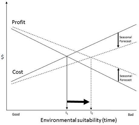
Figure 4. Benefit of seasonal forecasting under changing environmental suitability. In areas where the environmental suitability for the species under consideration is good, profits are high relative to costs. If the environmental suitability at a location declines over time under climate change, costs are expected to increase and profits decrease until a time at which a business would not be profitable (t1). Using seasonal forecasts to provide information on upcoming conditions, businesses should be able to reduce costs and increase profits, relative to no forecast such that they can remain profitable under less suitable environmental conditions for longer (until t₂). Beyond this point, conditions are such that relocation (or another adaptation option) is necessary.

A seasonal forecast system can only be useful if it produces reliable and accurate forecasts. For example, in southern Australia, model forecast skill, persistence forecast skill, and SST variability all vary across the region (Figure 5). Model skill here is quantified using Pearson's correlation, correlating monthly model and observed SST anomalies (i.e. deviations from the long-term monthly model/observed mean), where the observed dataset is Reynolds OISST v2 SST (Reynolds and Smith, 1994; Reynolds et al., 2002). A persistence forecast uses the current observed anomaly conditions as a predictor of future conditions; e.g., for a forecast beginning on 1 February 1990, the SST anomaly for January 1990 is used as the forecast and persisted for the duration of the forecast period (Spillman and Alves, 2009). In this example, persistence skill is quantified using Pearson's correlation, as per model skill. The performance of persistence forecasts is generally higher in areas of low intra-annual SST variability, i.e., where SST conditions vary little from month to month. For areas of low inter-annual monthly SST variability, i.e., SST for a particular month varies little from year to year, a climatological forecast (long-term monthly mean) can be useful.

FIGURE 5

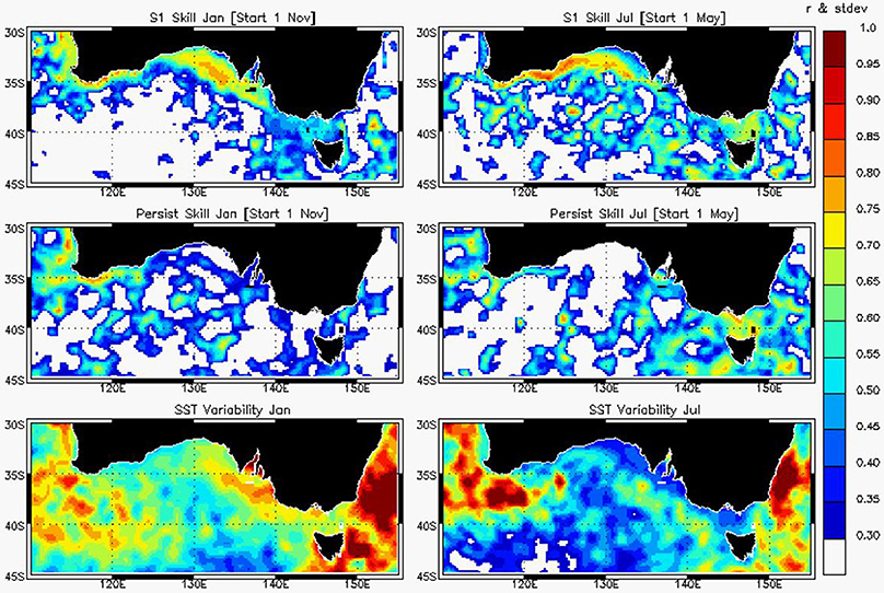
Figure 5. Skill of alternative seasonal forecast approaches in summer (January) and winter (July), illustrated for southern Australia. Row 1: skill for ACCESS-S1 forecasts issued 1 November and 1 May; Row 2: skill for persistence forecasts issued 1 November and 1 May; Row 3: inter-annual SST variability for January and July (standard deviation for January or July across 1991–2012). In all cases, values were calculated over the time period 1990–2012.

In the locations where inter-annual SST variability is low, such as during July in the inshore Great Australia Bight (~130–137°E) (Figure 5), a forecast may not be necessary (Case 1, Table 1). The most challenging case is when SST variability is high, and persistence and model skill is low. In these situations, forecasting may be very hard (Case 2, Table 1), such as in January off the Bonney Coast (~140°E), and real-time monitoring and rapid responses should be developed. If the persistence skill is high and model skill is low in a region (Case 3, Table 1), such as in July off south-west Western Australia (~115°E), real-time observations can also be used and future planning at a seasonal time scale based on the assumption that anomalous conditions will continue. These approaches (Cases 1–3, Table 1) are not climate-proof, as they do not account for trends in a changing environment. If model forecast skill is high (such as around Tasmania ~150°E in winter or in the Great Australian Bight ~130–137°E in summer), then a model forecast can be used in preference to a persistence forecast (whether high or low persistence skill and regardless of SST variability; Case 4 and Case 5, Table 1), since a dynamic model (e.g., ACCESS-S1) can account for trends in the changing environment and thus provides a climate-proof approach.

TABLE 1

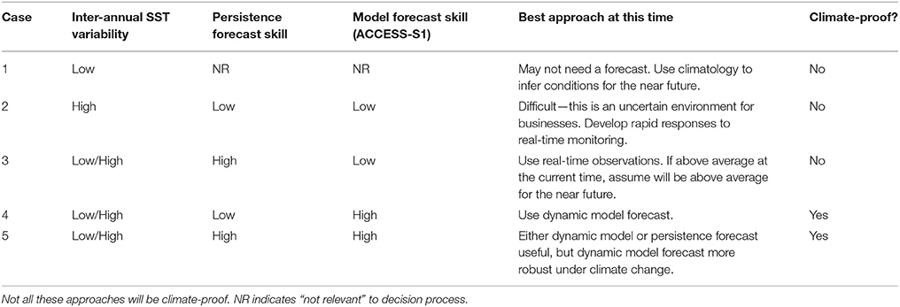
Table 1. Managing environmental variability at the present location is possible with several different approaches, depending on the historical environmental variability (in this case SST), the skill of a persistence forecast, and the skill of the dynamic model forecast.

Risk Management for Climate-Exposed Seafood Businesses

Marine industries, particularly seafood businesses, are exposed to environmental variability and long-term climate change, such that the future carries risks to production. While the focus here is on fisheries and aquaculture, this approach may also be useful for other applications: guiding external investment decisions in these marine industries; the insurance industry; and international seafood supply businesses that seek products from many regions who might be managing production risks across many locations in the same way that large agricultural companies manage supply chain risk.

Decision makers in aquaculture or marine management agencies often require information from a range of time scales in their decision making (Hobday et al., 2016; Tommasi et al., 2017). Fisheries managers can use forecast information to plan distribution of fishing effort, as has been proposed for the Californian sardine fishery based on forecasts with a downscaled regional ocean model (Kaplan et al., 2016). Aquaculture managers might be charged with managing production and harvest schedules, which can be informed by knowledge of likely (and unlikely) conditions over the coming months (i.e., seasonal forecasts). At longer time scales, they may use climate-scale forecasts to assess the need to seek new sites, and if necessary, to negotiate with coastal planning agencies for access to new regions. In the same way, coastal management agencies may use long-term climate projections to develop zoning plans.

While more mobile than aquaculture, fisheries are still relatively site attached with regard to access to fixed infrastructure such as ports, product transport and processing plants; thus, information on future environmental conditions at a local scale is still important for short and long-term planning. For example, the southern bluefin tuna (SBT) fishery in the Great Australia Bight currently utilizes seasonal forecasts to plan the timing and location of fishing operations, workforce management, and equipment deployment (Eveson et al., 2015). This fishery is more site-attached than most in that captured fish are towed back to farm sites near Port Lincoln, South Australia, for grow-out in cages (Ellis and Kiessling, 2016). If climate change results in conditions at the current catch locations becoming unsuitable for SBT, fish may move too far from the farm sites for this system to be viable. Alternatively, conditions at the farm sites could become unsuitable. In both cases, climate forecasts could be used to assess future viability of alternative farm sites, with seasonal forecasts used in the interim to manage risks due to changing fish distribution or unsuitable grow-out conditions.

For marine industries provided with environmental information about the future, such as warming waters in the examples presented here, there are a range of risk management options. Most simplistic is a movement to new regions that meet the required environmental conditions. Given the long-term persistence of climate change (e.g., many centuries of temperature and sea level rise; Meehl et al., 2012), industries may have to relocate more than once in the future to stay within an environmental suitability envelope. If the changes are such that relocation is not possible or not cost-effective, an adaptation response could be to change the focal species of the fishery or aquaculture operation. For example, in eastern Tasmania, SST conditions may begin to suit other species for farming or wild fisheries, such as kingfish (Seriola lalandi). This species is currently exploited by aquaculture and fishery industries further north in Australia, and its distribution is already expanding further south (Stuart-Smith et al., 2016).

Here we have focused on SST as a dominant driver of marine production, but the same approach could be used for other critical variables such as upwelling strength, eddy activity, oxygen concentration or primary production. In order to deliver information for variables that have greater spatial variability and projection uncertainty, seasonal and climate models will need to improve and be validated. Thus, any decisions made on the basis of climate forecasts available today may need to be revisited with revised forecasts over the coming years, as predictive skill improves. While we have considered just a single set of climate projections and a single variable (SST), other studies show that the uncertainty of climate scale forecasts can be relatively large, and this uncertainty increases further into the future (Payne et al., 2017). Thus, a business may need to deal with the case where the upper temperature threshold for their species/situation is expected to be permanently exceeded anywhere from, say, 2040 to 2060. This is where the power of considering seasonal forecasting at the same time is demonstrated. The risk due to uncertainty with long-term projections (i.e., conditions will become unsuitable, but when?) can be reduced with information on shorter time scales.

Additional research is needed to evaluate the cost-benefit of future climate-proofing, such as examining the risk of following a new strategy too soon. For example, a pre-emptive move from warming conditions may result in a better environment for the activity, but may result in a business being too far from existing infrastructure. Integrated responses to climate risk are needed, with strong engagement across the range of stakeholders involved, from the primary fishers to the managers and policy makers. All these groups should work together to consider the appropriate responses to future climate risk, how it can be reduced with future information, and how to plan for transitions to new ways of doing business. Providing information for regional planning agencies is particularly important, as many government agencies have not yet begun to recognize the need for changes in the regional marine industries. Long-term projections can help with development of parallel responses. Thus, a combination of seasonal and long-term forecasting tools will allow entire regions to undergo spatial planning at time scales previously considered separately.

Author Contributions

AH and CS: Conceived paper; XZ: Contributed analyses; AH, CS, JE, JH, XZ and SB: All co-wrote paper.

Conflict of Interest Statement

The authors declare that the research was conducted in the absence of any commercial or financial relationships that could be construed as a potential conflict of interest.

Acknowledgments

We thank Faina Tseitkin, Griffith Young, and Guo Liu (Bureau of Meteorology, Australia) for preparing the ACCESS-S1 hindcasts, and Debbie Hudson and Oscar Alves (Bureau of Meteorology) for their comments and review of previous versions of the manuscript. The climate model downscaling results were produced by the Ocean Downscaling Strategic Project, funded by CSIRO Oceans and Atmosphere, in close collaboration with the Bluelink team (http://wp.csiro.au/bluelink/global/). This paper is a contribution from the CLIOTOP task team on seasonal and decadal forecasting. We appreciate the comments made by the reviewers that helped us to improve the manuscript.

References

Battaglene, S. C., Carter, C., Hobday, A. J., Lyne, V., and Nowak, B. (2008). Scoping Study Into Adaptation of the Tasmanian Salmonid Aquaculture Industry to Potential Impacts of Climate Change. National Agriculture and Climate Change Action Plan: Implementation Programme report. 83.

Bell, J. D., Ganachaud, A., Gehrke, P. C., Griffiths, S. P., Hobday, A. J., Hoegh-Guldberg, O., et al. (2013). Mixed responses of tropical Pacific fisheries and aquaculture to climate change. Nat. Clim. Change 3, 591–599. doi: 10.1038/nclimate1838

CrossRef Full Text | Google Scholar

Bennett, S., Wernberg, T., Connell, S. D., Hobday, A. J., Johnson, C. R., and Poloczanksa, E. S. (2016). The ‘Great Southern Reef’: social, ecological and economic value of Australia's neglected kelp forests. Mar. Freshwater Res. 67, 47–56. doi: 10.1071/MF15232

CrossRef Full Text | Google Scholar

Brander, K. (2013). Climate and current anthropogenic impacts on fisheries. Clim. Change 119, 9–21. doi: 10.1007/s10584-012-0541-2

CrossRef Full Text | Google Scholar

Brodie, S., Hobday, A. J., Smith, J. A., Spillman, C. M., Hartog, J. R., Everett, J. D., et al. (2017). Seasonal forecasting of dolphinfish distribution in eastern Australia to aid recreational fishers and managers. Deep Sea Res. II. 140, 229–239. doi: 10.1016/j.dsr2.2017.03.004

CrossRef Full Text | Google Scholar

Callaway, R. M., Shinn, A. P., Grenfell, S. E., Bron, J. E., Burnell, G., Cook, E. J., et al. (2012). Review of climate change impacts on marine aquaculture in the UK and Ireland. Aquat. Conserv. Mar. Freshw. Ecosyst. 22, 389–421. doi: 10.1002/aqc.2247

CrossRef Full Text | Google Scholar

Chang, Y., Lee, M., Lee, K., and Shao, K. (2013). Adaptation of fisheries and mariculture management to extreme oceanic environmental changes and climate variability in Taiwan. Mar. Policy 38, 476–482. doi: 10.1016/j.marpol.2012.08.002

CrossRef Full Text | Google Scholar

Cheung, W. W. L., Lam, V. W. Y., Sarmiento, J. L., Kearney, K., Watson, R., Zeller, D., et al. (2010). Large-scale redistribution of maximum fisheries catch potential in the global ocean under climate change. Glob. Change Biol. 16, 24–35. doi: 10.1111/j.1365-2486.2009.01995.x

CrossRef Full Text | Google Scholar

Dell, J. T., Wilcox, C., Matear, R. J., Chamberlain, M. A., and Hobday, A. J. (2015). Potential impacts of climate change on the distribution of longline catches of yellowfin tuna (Thunnus albacares) in the Tasman Sea. Deep Sea Res. II 113, 235–245. doi: 10.1016/j.dsr2.2014.07.002

CrossRef Full Text | Google Scholar

Ellis, D., and Kiessling, I. (2016). “Ranching of Southern Bluefin Tuna in Australia,” in Advances in Tuna Aquaculture. eds D. D. Benetti, G. J. Partridge, and A. Buentello (Tokyo: Elsevier), 217–232.

Google Scholar

Eveson, J. P., Hobday, A. J., Hartog, J. R., Spillman, C. M., and Rough, K. M. (2015). Seasonal forecasting of tuna habitat in the Great Australian Bight. Fish. Res. 170, 39–49. doi: 10.1016/j.fishres.2015.05.008

CrossRef Full Text | Google Scholar

Frusher, S. D., van Putten, E. I., Haward, M., Hobday, A. J., Holbrook, N. J., Jennings, S., et al. (2016). From physics to folk via fish – connecting the socio-ecological system to understand the ramifications of climate change on coastal regional communities. Fish. Oceanogr. 25, 19–28. doi: 10.1111/fog.12139

CrossRef Full Text | Google Scholar

Griffies, S. M. (2009). Elements of MOM4p1, GFDL Ocean Group. Technical Report 6. NOAA/Geophysical Fluid Dynamics Laboratory.

Hartog, J., Hobday, A. J., Matear, R., and Feng, M. (2011). Habitat overlap of southern bluefin tuna and yellowfin tuna in the east coast longline fishery - implications for present and future spatial management. Deep Sea Res. II 58, 746–752. doi: 10.1016/j.dsr2.2010.06.005

CrossRef Full Text | Google Scholar

Hawkins, E., and Sutton, R. (2012). Time of emergence of climate signals. Geophys. Res. Lett. 39:L01702. doi: 10.1029/2011GL050087

CrossRef Full Text | Google Scholar

Hobday, A. J. (2010). Ensemble analysis of the future distribution of large pelagic fishes in Australia. Prog. Oceanogr. 86, 291–301 doi: 10.1016/j.pocean.2010.04.023

CrossRef Full Text | Google Scholar

Hobday, A. J., Hartog, J., Spillman, C., and Alves, O. (2011). Seasonal forecasting of tuna habitat for dynamic spatial management. Can. J. Fish. Aquat. Sci. 68, 898–911. doi: 10.1139/f2011-031

CrossRef Full Text | Google Scholar

Hobday, A. J., and Lough, J. (2011). Projected climate change in Australian marine and freshwater environments. Mar. Freshw. Res. 62, 1000–1014. doi: 10.1071/MF10302

CrossRef Full Text | Google Scholar

Hobday, A. J., and Pecl, G. T. (2014). Identification of global marine hotspots: sentinels for change and vanguards for adaptation action. Rev. Fish Biol. Fish. 24, 415–425. doi: 10.1007/s11160-013-9326-6

CrossRef Full Text | Google Scholar

Hobday, A. J., Spillman, C. M., Eveson, J. P., and Hartog, J. R. (2016). Seasonal forecasting for decision support in marine fisheries and aquaculture. Fish. Oceanogr. 25, 45–56. doi: 10.1111/fog.12083

CrossRef Full Text | Google Scholar

Hudson, D., Shi, L., Alves, O., Zhao, M., Hendon, H., and Young, G. (2017). Performance of ACCESS-S1 for Key Horticultural Regions. Bureau Research Report, No. 20. Bureau of Meteorology Australia. Available online at: http://www.bom.gov.au/research/research-reports.shtml

Kaplan, I. C., Williams, G. D., Bond, N. A., Hermann, A. J., and Siedlecki, S. (2016). Cloudy with a chance of sardines: forecasting sardine distributions using regional climate models. Fish. Oceanogr. 25, 15–27. doi: 10.1111/fog.12131

CrossRef Full Text | Google Scholar

Kates, R. W., Travis, W. R., and Wilbanks, T. J. (2012). Transformational adaptation when incremental adaptations to climate change are insufficient. Proc. Natl. Acad. Sci. U.S.A. 109, 7156–7161. doi: 10.1073/pnas.1115521109

PubMed Abstract | CrossRef Full Text | Google Scholar

Kobayashi, S., Ota, Y., Harada, Y., Ebita, A., Moriya, M., Onoda, H., et al. (2015), The JRA-55 Reanalysis: general specifications basic characteristics. J. Meteorol. Soc. Japan 93, 5–48. doi: 10.2151/jmsj.2015-001

CrossRef Full Text | Google Scholar

Lehodey, P., Alheit, J., Barange, M., Baumgartner, T. R., Beaugrand, G., Drinkwater, K., et al. (2006). Climate variability, fish, and fisheries. J. Clim. 19, 5009–5030. doi: 10.1175/JCLI3898.1

CrossRef Full Text | Google Scholar

Lehodey, P., Senina, I., Sibert, J., Bopp, L., Calmettes, B., Hampton, J., et al. (2010). Preliminary forecasts of Pacific bigeye tuna population trends under the A2 IPCC scenario. Prog. Oceanogr. 86, 302–315. doi: 10.1016/j.pocean.2010.04.021

CrossRef Full Text | Google Scholar

Lim, E. P., Hendon, H. H., Hudson, D., Zhao, M., Shi, L., and Alves, O., et al. (2016) Evaluation of the ACCESS-S1 Hindcasts for Prediction of Victorian Seasonal Rainfall. Bureau Research Report, No. 19. Bureau of Meteorology, Australia. Available online at: http://www.bom.gov.au/research/research-reports.shtml

Little, L. R., Hobday, A. J., Parslow, J. S., Davies, C. R., and Grafton, R. Q. (2015). Funding climate adaptation strategies with climate derivatives. Clim. Risk Manage. 8, 9–15. doi: 10.1016/j.crm.2015.02.002

CrossRef Full Text | Google Scholar

Lyu, K., Zhang, X., Church, J. A., Slangen, A. B. A., and Hu, J. (2014). Time of emergence for regional sea-level change. Nat. Clim. Change 4, 1006–1010. doi: 10.1038/nclimate2397

CrossRef Full Text | Google Scholar

Madin, E. M. P., Ban, N., Doubleday, Z. A., Holmes, T. H., Pecl, G. T., and Smith, F. (2012). Socio-economic and management implications of range-shifting species in marine systems. Global Environ. Change 22, 137–146. doi: 10.1016/j.gloenvcha.2011.10.008

CrossRef Full Text | Google Scholar

Meehl, G. A., Hu, A., Tebaldi, C., Arblaster, J. M., Washington, W. M., Teng, H., et al. (2012). Relative outcomes of climate change mitigation related to global temperature versus sea-level rise. Nat. Clim. Change 2, 576–580. doi: 10.1038/nclimate1529

CrossRef Full Text | Google Scholar

Oke, P. R., Griffin, D. A., Schiller, A., Matear, R. J., Fiedler, R., Mansbridge, J., et al. (2013) Evaluation of a near-global eddy-resolving ocean model, Geosci. Model Dev. 6, 591–615. doi: 10.5194/gmd-6-591-2013

CrossRef Full Text | Google Scholar

Oliver, E. C. J., Benthuysen, J. A., Bindoff, N. L., Hobday, A. J., Holbrook, N. J., Mundy, C. N., et al. (2017). The unprecedented 2015/16 Tasman Sea marine heatwave. Nat. Commun. 8:16101. doi: 10.1038/ncomms16101

PubMed Abstract | CrossRef Full Text | Google Scholar

Oliver, E. C. J., Wotherspoon, S., Chamberlain, M. A., and Holbrook, N. J. (2014). Projected Tasman sea extremes in sea surface temperature through the twenty-first century. J. Clim. 27, 1980–1998. doi: 10.1175/JCLI-D-13-00259.1

CrossRef Full Text | Google Scholar

Payne, M. R., Hobday, A. J., MacKenzie, B. R., Tommasi, D., Dempsey, D. P., Fässler, S. M. M., et al. (2017). Lessons from the first generation of marine ecological forecasts products. Front. Mar. Sci. 4:289. doi: 10.3389/fmars.2017.00289

CrossRef Full Text | Google Scholar

Popova, E. E., Yool, A., Byfield, V., Cochrane, K., Coward, A., Icar, S., et al. (2016). From global to regional and back again: unifying mechanisms of climate change relevant for adaptation across five ocean warming hotspots. Glob. Chang. Biol. 22, 2038–2053. doi: 10.1111/gcb.13247

CrossRef Full Text | Google Scholar

Reynolds, R. W., Rayner, N. A. T., Smith, M., Stokes, D. C., and Wang, W. (2002). An improved in-situ and satellite SST analysis for climate. J. Clim. 15, 1609–1625. doi: 10.1175/1520-0442(2002)015<1609:AIISAS>2.0.CO;2

CrossRef Full Text | Google Scholar

Reynolds, R. W., and Smith, T. M. (1994). Improved global sea surface temperature analyses. J. Clim. 7, 929–948. doi: 10.1175/1520-0442(1994)007<0929:IGSSTA>2.0.CO;2

CrossRef Full Text | Google Scholar

Robinson, L., Hobday, A. J., Possingham, H. P., and Richardson, A. J. (2015). Trailing edges projected to move faster than leading edges for large pelagic fish under climate change. Deep Sea Res. II 113, 225–234. doi: 10.1016/j.dsr2.2014.04.007

CrossRef Full Text | Google Scholar

Savage, J., and Hobsbawn, P. (2015). Australian fisheries and aquaculture statistics 2014, Fisheries Research and Development Corporation Project 2014/245. Canberra, ACT: ABARES.

Salinger, J., Hobday, A. J., Matear, R. J., O'Kane, T. J., Risbey, J. S., Dunstan, P., et al. (2016). Chapter One - Decadal-scale forecasting of climate drivers for marine applications. Adv. in Marine Biol. 74, 1–68. doi: 10.1016/bs.amb.2016.04.002

CrossRef Full Text | Google Scholar

Spillman, C. M., and Alves, O. (2009). Dynamical seasonal prediction of summer sea surface temperatures in the great barrier reef. Coral Reefs 28, 197–206. doi: 10.1007/s00338-008-0438-8

CrossRef Full Text | Google Scholar

Spillman, C. M., Hartog, J. R., Hobday, A. J., and Hudson, D. (2015). Predicting environmental drivers for prawn aquaculture production to aid improved farm management. Aquaculture 447, 56–65. doi: 10.1016/j.aquaculture.2015.02.008

CrossRef Full Text | Google Scholar

Spillman, C. M., and Hobday, A. J. (2014). Dynamical seasonal forecasts aid salmon farm management in an ocean warming hotspot. Clim. Risk Manage. 1, 25–38. doi: 10.1016/j.crm.2013.12.001

CrossRef Full Text | Google Scholar

Stock, C. A., Alexander, M. A., Bond, N. A., Brander, K. M., Cheung, W. W. L., Curchitser, E. N., et al. (2011). On the use of IPCC-class models to assess the impact of climate on living marine resources. Prog. Oceanogr. 88, 1–27. doi: 10.1016/j.pocean.2010.09.001

CrossRef Full Text | Google Scholar

Stuart-Smith, J. F., Pecl, G., Pender, A., Tracey, S., Villanueva, C., and Smith-Vaniz, W. F. (2016). Southernmost records of two Seriola species in an Australian ocean-warming hotspot. Mar. Biodivers. doi: 10.1007/s12526-016-0580-4

CrossRef Full Text | Google Scholar

Taylor, K. E., Stouffer, R. J., and Meehl, G. A. (2012) An overview of CMIP5 the experiment design. Bull. Am. Meteorol. Soc. 93, 485–498. doi: 10.1175/BAMS-D-11-00094.1

CrossRef Full Text | Google Scholar

Tommasi, D., Stock, C., Hobday, A. J., Methot, R., Kaplan, I., Eveson, P., et al. (2017). Managing living marine resources in a dynamic environment: the role of seasonal to decadal climate forecasts. Prog. Oceanogr. 152, 15–49. doi: 10.1016/j.pocean.2016.12.011

CrossRef Full Text | Google Scholar

Zhang, X., Oke, P., Feng, M., Chamberlain, M., Church, J., Monselesan, D., et al. (2016). A near-global eddy-resolving OGCM for climate studies. Geosci. Model Dev. Discuss. doi: 10.5194/gmd-2016-17

CrossRef Full Text | Google Scholar

Zhang, X., Church, J. A., Monselesan, D., and McInnes, K. L. (2017). Sea level projections for the Australian region in the 21st century. Geophys. Res. Lett. 44, 8481–8491. doi: 10.1002/2017GL074176

CrossRef Full Text | Google Scholar