Optical Modeling of Spectral Backscattering and Remote Sensing Reflectance From Emiliania huxleyi Blooms

Introduction

Coccolithophores are phytoplankton that form an exoskeleton of calcite scales called coccoliths (Figure 1). They are major oceanic calcite producers and carbon exporters in the ocean (Iglesias-Rodríguez et al., 2002; Broecker and Clark, 2009). The cosmopolitan coccolithophore species Emiliania huxleyi (Lohmann) Hay & Mohler thrives from tropical to subpolar oceans and forms large-scale, intense blooms particularly in temperate waters (Tyrrell and Merico, 2004). In the later bloom stages E. huxleyi overproduces and sheds coccoliths, giving the ocean a bright milky-turquoise appearance, which makes these blooms easily discernible from optical satellites (Groom and Holligan, 1987; Holligan et al., 1993; Brown and Yoder, 1994), especially ocean color satellites (Gordon et al., 2001; Balch et al., 2005). The backscattering of light by coccoliths and coccospheres forms the basis of the remote sensing algorithm for the retrieval of the concentration of particulate inorganic carbon, PIC (see Table 1 for a list of symbols and abbreviations), or calcite (Gordon et al., 2001; Balch et al., 2005). Remotely sensed PIC has been widely used to study coccolithophore bloom extent, occurrence, and timing in the global ocean (Balch et al., 2011; Hopkins et al., 2015), as well as their poleward expansion in response to climate change (Winter et al., 2014; Neukermans et al., 2018).

FIGURE 1

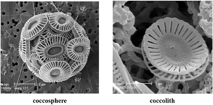
Figure 1. Scanning Electron Micrograph of Emiliania huxleyi (Dr. Jeremy Young, University College London, London, with permission).

TABLE 1

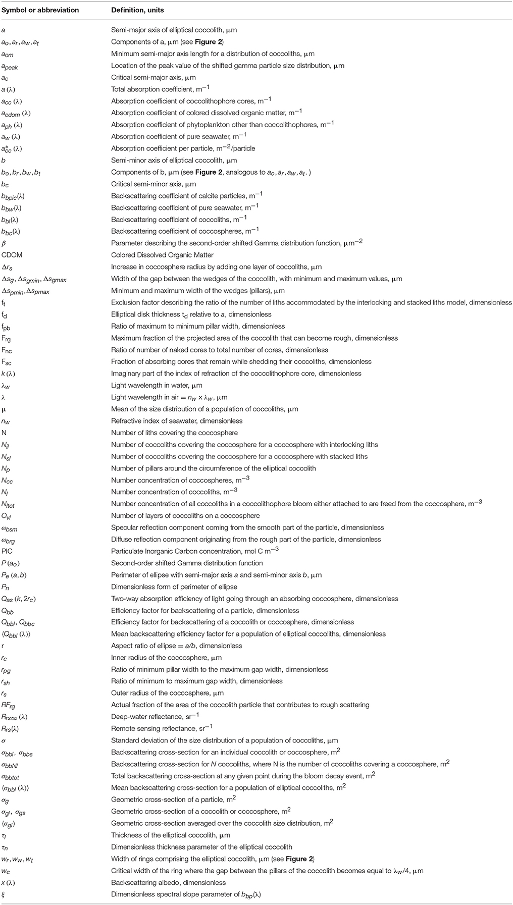
Table 1. List of abbreviations, symbols, definitions, and units.

In situ and laboratory observations show that the relationship between light backscattering and PIC may vary, however, and the causes for this variability are poorly understood (e.g., Balch et al., 1991). While it is commonly assumed that PIC-specific light backscattering (=backscattering per unit PIC) is orders of magnitude higher for detached coccoliths than for coccospheres (Balch et al., 1991, 1996), Gordon et al. (2009) suggested that this would not be so based on a comparison of an optical model and in situ measurements in a coccolithophore bloom. Optical models are indeed useful to investigate variations in light backscattering due to changes in size and morphology of coccoliths and coccospheres, but investigations have been limited due to the computational demand of commonly used optical models suitable for light backscattering such as the discrete dipole approximation (Gordon and Du, 2001; Gordon, 2006; Zhai et al., 2013). Recently, however, Fournier and Neukermans (2017) developed an analytical optical model for light backscattering from coccoliths and coccolithophores of E. huxleyi. Our previous model closely matched results obtained from the discrete dipole approximation computations of Zhai et al. (2013) in which E. huxleyi coccoliths were represented as two thin circular disks attached together by a tube and perforated by a set of wedge shaped openings.

In the present paper we first improve our previous analytical optical model to account for a more realistic representation of the morphology of E. huxleyi coccoliths and coccospheres. More specifically we account for (i) the fact that coccoliths are elliptical in shape with triangularly shaped wedge openings (Figure 1), and (ii) detailed coccosphere architecture with interlocking coccoliths as obtained from three dimensional electron microscopy observations of E. huxleyi coccolithophores (Hoffmann et al., 2015). We then improve our previous size distribution model based on detailed analyses of observed coccolith size distributions (Young et al., 2014). Using our new coccolithophore and coccolith backscattering model and an algebraic radiative transfer model we investigate the variability in spectral backscattering and ocean color remote sensing reflectance (i) due to changes in E. huxleyi coccolith size distribution and morphology, (ii) due to changes in the ratio of free to attached coccoliths, and (iii) during a hypothetical bloom decay event in which E. huxleyi sheds its attached liths. Programming codes for all computations in this paper are provided in Neukermans and Fournier (2018), including future releases.

Methods

The light backscattering coefficient of calcite particles suspended in seawater, b_bpic (in m⁻¹, see Table 1 for a list of symbols and units), can be partitioned in its contributions from liths and coccospheres, represented by b_bl and b_bc, respectively:

$\begin{array}{ll}{b}_{bpic}=b_{bl}+b_{bc}& (1)\end{array}$

For populations of identical coccoliths and coccospheres we can write:

$\begin{array}{ll}{b}_{bpic}=N_l{\sigma }_{bbl}+N_{cc}{\sigma }_{bbs}& (2)\end{array}$

where N_l and N_cc are the number concentrations of coccoliths and coccospheres (in m⁻³), respectively, and σ_bbl and σ_bbs are the corresponding backscattering cross-sections for individual coccoliths and coccospheres (in m²). The backscattering cross-section is defined as the product of the geometric cross-section of the calcite particle σ_g (in m²) and the dimensionless efficiency factor for backscattering of the particle Q_bb so that:

$\begin{array}{ll}{\sigma }_{bbl}=Q_{bbl}{\sigma }_{gl}\text{and}{\sigma }_{bbs}=Q_{bbs}{\sigma }_{gs}& (3)\end{array}$

where the efficiency factor Q_bb is the ratio of radiant power backscattered by the particle to radiant power intercepted by the geometric cross-section of the particle (e.g., Morel and Bricaud, 1986).

The underlying assumptions to Equation (3) are, first, that coccoliths and coccolithophores are randomly oriented with respect to the direction of incident light. This allows us to evaluate σ_g through the theorem of Cauchy (1850) which states that the average σ_g of a randomly oriented particle of convex shape is equal to a quarter of its surface area. Second, for coccolithophores and coccoliths made of high refractive index calcite material, the backscattering efficiency Q_bb is dominated by the contribution of reflection from the particle surface (Fournier and Neukermans, 2017). For an ensemble of randomly oriented reflecting surfaces the theorem of van de Hulst (1957) formally states that: “the [angular] scattering pattern caused by reflection on large convex particles with random orientation is identical with the [angular] scattering pattern of a large sphere made of the same material and with the same surface condition.” This equivalence is a direct consequence of the angular averaging procedure, which holds for randomly oriented surfaces. Therefore, it follows that the unity-normalized angular distribution of reflection from a randomly oriented convex body is shape-independent and can be characterized by a single scattering phase function in the back-direction. This allows us to treat orientation averages of the scattering efficiency factor and the geometric cross-section separately, which is implicitly assumed in Equation (3). In short, for randomly oriented highly reflective particles such as coccoliths and coccolithophores, the average σ_bb can be obtained by multiplying σ_g with Q_bb.

In what follows we first develop expressions for σ_bbl for single coccoliths (section Model for the Backscattering Cross-Section of an Elliptical Coccolith) as a function of lith size, shape, and morphology. We thereby build on our previous modeling work (Fournier and Neukermans, 2017) which relies on the fundamental hypothesis that for particles large compared to the wavelength of light, the backscattering is dominated by the reflection from the surfaces of the particles. This approximation holds particularly well for coccoliths because they are made of calcite, a material with a refractive index of 1.2 relative to water and therefore a high reflection coefficient. The reflection from the four calcite surfaces which comprise the coccolith particle is considered to be specular, and the surfaces are assumed smooth when the surface roughness features are smaller than a quarter of the light wavelength in water, λ_w. If the surface roughness features become larger than λ_w/4, light is reflected diffusely. This is represented in our previously derived formula for the backscattering efficiency of a single circular coccolith particle:

$\begin{array}{ll}{Q}_{bbl}={\omega }_{bsm}\left(1-R{F}_{rg}\right)+{\omega }_{brg}R{F}_{rg}& (4)\end{array}$

where F_rg is the maximum fraction of the projected area of the particle that can become rough, RF_rg is the actual fraction of the area of the particle that contributes to rough scattering, ω_bsm represents the specular reflection component coming from the smooth part of the particle surface and ω_brg is a diffuse reflection component originating from the rough part of the particle surface. Expressions for ω_brg and ω_bsm as functions of the refractive index are derived in Fournier and Neukermans (2017).

Model for the Backscattering Cross-Section of an Elliptical Coccolith

To model the light backscattering cross-section of an elliptical coccolith of E. huxleyi we need to derive Q_bbl and σ_gl (Equation 3) and therefore we need to consider the detailed geometry of a coccolith (Young et al., 2014) which is schematically depicted in Figure 2. The semi-major axis a is ½ the coccolith length while the semi-minor axis b is ½ the coccolith width. As indicated in Figure 2, the structure of the coccolith can be accurately represented by a set of four ellipses separated by three rings of fixed width. We have an outermost ellipse separated by a thin ring of width w_r from the ellipse which marks the beginning of the zone with the open wedges. This ellipse is in turn separated by a ring of width w_w from an inner ellipse. These ellipses define the boundaries of the lith area containing the wedged openings. The inner ellipse is separated from a center ellipse by a width w_t that represents the boundaries of the inner tube joining the distal and proximal sheets.

FIGURE 2

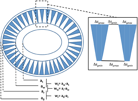
Figure 2. Schematic representation of the morphology of an E. huxleyi coccolith as measured by Young et al. (2014). The inset describes details of the wedge structure of the openings.

The average geometric cross-section of a randomly oriented elliptical coccolith is derived in Supplementary Information section 1.1 (based on Cauchy, 1850's theorem) and repeated here for convenience:

$\begin{array}{ll}{\sigma }_{gl}=\left(\frac{1}{4}\right)\left[2\pi \left(ab\right)+{\tau }_l{P}_e\left(a,b\right)\right]& (5)\end{array}$

where τ_l is the thickness of the elliptical disk and P_e(a, b) its perimeter with equations given in Supplementary Information section 1.1.

We can represent the proportional relations between the various ellipse parameters (a_o, a_r, a_w, a_t) and (b_o, b_r, b_w, b_t) as follows (Figure 2):

$\begin{array}{l}\frac{a_r}{a_o}=\left[1-\frac{w_r}{a_0}\right]\text{and}\frac{b_r}{b_o}=\left[1-\left(\frac{a_o}{b_o}\right)\frac{w_r}{a_o}\right]\\ \frac{a_w}{a_o}=\left[1-\frac{\left(w_r+w_w\right)}{a_0}\right]\text{and}\frac{b_w}{b_o}=\left[1-\left(\frac{a_o}{b_o}\right)\frac{\left(w_r+w_w\right)}{a_o}\right]\\ \frac{a_t}{a_o}=\left[1-\frac{\left(w_r+w_w+w_t\right)}{a_0}\right]\text{and}\frac{b_t}{b_o}=\left[1-\left(\frac{a_o}{b_o}\right)\frac{\left(w_r+w_w+w_t\right)}{a_o}\right]& (6)\end{array}$

For the coccolith in Figure 1, with major axis in μm of a_o = 1.8688, we have the following proportionalities:

$\begin{array}{l}\frac{a_o}{b_o}=r_0=1.20\\ \frac{w_r}{a_0}=0.0439\\ \frac{w_w}{a_0}=0.3158\\ \frac{w_t}{a_0}=0.1688\end{array}$

The maximum fraction of the surface area of the coccolith that can become rough F_rg lies between ellipses with parameters (a_r, a_w) and (b_r, b_w) so we can write:

$\begin{array}{ll}{F}_{rg}=\left[\frac{a_r}{a_o}\frac{b_r}{b_o}-\frac{a_w}{a_o}\frac{b_w}{b_o}\right]& (7)\end{array}$

which gives F_rg = 0.5418 for the coccolith in Figure 2.

We will now analyze more closely the structure of wedges and pillars. The structure of the wedges and pillars in the zone between a_r and a_w can be represented as a set of gaps with maximum widths Δs_gmax and minimum pillar width Δs_pmin respectively along the elliptical boundary at a_r and minimum widths Δs_gmin and maximum pillar width Δs_pmax. The gap width narrows down to Δs_gmin on the elliptical boundary at a_w while the pillar width grows to fill the empty space. Given N_p pillars around the circumference of the ellipse at a_r we have:

$\begin{array}{l}{N}_p\left(\Delta s_{gmax}+\Delta s_{pmin}\right)=P_e\left(a_r,b_r\right)\\ N_p\left(\Delta s_{gmin}+\Delta s_{pmax}\right)=P_e\left(a_w,b_w\right)& (8)\end{array}$

Defining the ratio of the minimum pillar width to the maximum gap width, r_pg, and the ratio of minimum to maximum gap width, r_sh, as:

$\begin{array}{ll}{r}_{pg}=\frac{\Delta s_{pmin}}{\Delta s_{gmax}}\text{and}{r}_{sh}=\frac{\Delta s_{gmin}}{\Delta s_{gmax}}& (9)\end{array}$

we obtain the following expression for Δs_gmax

$\begin{array}{ll}\Delta s_{gmax}=\frac{P_e\left(a_r,b_r\right)}{N_p\left(1+r_{pg}\right)}=\frac{2\pi a_0{P}_n\left(\frac{a_r}{a_o},\frac{b_r}{a_o}\right)}{N_p\left(1+r_{pg}\right)}& (10)\end{array}$

where P_n is the dimensionless ellipse perimeter given in Equation (S13). As we proceed from the ellipse at a_r to the ellipse at a_w the gap Δs_g narrows from Δs_gmax to Δs_gmin as w goes from 0 to w_w

$\begin{array}{ll}\Delta s_g=\Delta s_{gmax}\left[1-\left(1-r_{sh}\right)\frac{w}{w_w}\right]& (11)\end{array}$

To determine where the backscattering becomes rough we need to compute at what value of a the gap Δs_g becomes equal to 1/4 of λ_w (Gordon, 2006; Fournier and Neukermans, 2017). We define w_c as the critical width where the gap becomes equal to λ_w/4, then Equation (11) gives:

$\begin{array}{ll}\frac{{\lambda }_w}{4}=\Delta s_{gmax}\left[1-\left(1-r_{sh}\right)\frac{w_c}{w_w}\right]& (12)\end{array}$

The corresponding critical semi-major axis a_c and semi-minor axis b_c are given by:

$\begin{array}{ll}{a}_c=a_o-\left(w_r+w_c\right)\text{or}\frac{a_c}{a_o}=\left[1-\frac{\left(w_r+w_c\right)}{a_o}\right]& (13)\end{array}$

$\begin{array}{ll}{b}_c=b_o-\left(w_r+w_c\right)\text{or}\frac{b_c}{b_o}=\left[1-\left(\frac{a_o}{b_o}\right)\frac{\left(w_r+w_c\right)}{a_o}\right]& (14)\end{array}$

As long as the gap Δs_g is smaller than Δs_gmax and larger than λ_w/4 we can compute the critical width as:

$\begin{array}{ll}{w}_c=w_w\frac{\left(1-\frac{{\lambda }_w/4}{\Delta s_{gmax}}\right)}{\left(1-r_{sh}\right)}\text{for}\frac{{\lambda }_w}{(4\Delta s_g)}\le 1& (15)\end{array}$

When Δs_g is smaller than $\frac{{\lambda }_w}{4}$ we must set w_c to 0 and on the high side as the wavelength gets smaller we must limit w_c to a maximum value of w_w:

$\begin{array}{ll}{w}_c=0\text{for}\frac{{\lambda }_w/4}{\Delta s_g}>1\text{and}{w}_c=w_w\text{for}\frac{\left(1-\frac{{\lambda }_w/4}{\Delta s_{gmax}}\right)}{\left(1-r_{sh}\right)}>1& (16)\end{array}$

We can then proceed to compute the ratio $\frac{w_c}{a_o}$ which is required to evaluate the fraction of rough surface of the coccolith using Equations (15) and (10).

$\begin{array}{l}\frac{w_c}{a_o}=\frac{w_w}{a_o}\left(\frac{1}{1-r_{sh}}\right)\left(1-\frac{{\lambda }_w/4}{\Delta s_{gmax}}\right)\\ =\frac{w_w}{a_o}\left(\frac{1}{1-r_{sh}}\right)\left[1-\left(\frac{{\lambda }_w}{4\pi a_o}\right)\frac{N_p\left(1+r_{pg}\right)}{P_n\left(\frac{a_r}{a_o},\frac{b_r}{a_o}\right)}\right]& (17)\end{array}$

Substituting this expression in Equations (13) and (14) we obtain directly the fraction of the elliptical surface of the coccolith that is rough:

$\begin{array}{ll}R{F}_{rg}\left(a_o,\lambda \right)=\frac{\pi a_r{b}_r-\pi a_c{b}_c}{\pi a_o{b}_o}=\left[\frac{a_r}{a_o}\frac{b_r}{b_o}-\frac{a_c}{a_o}\frac{b_c}{b_o}\right]& (18)\end{array}$

The only variable determining the behavior of RF_rg is the ratio of the wavelength in water λ_w to the major axis a_o of the elliptical coccolith. The rest of the elements are fixed by the proportionality factors dictated by the assumed shape of the coccolith.

Combining Equations (8) and (9) we find for the ratio of circumferences of the outer and inner ellipse where the wedges and pillars occur:

$\begin{array}{ll}\frac{P_e\left(a_w,b_w\right)}{P_e\left(a_r,b_r\right)}=\frac{1}{1+r_{pg}}\left(r_{sh}+\frac{\Delta s_{pmax}}{\Delta s_{gmax}}\right)=\frac{1}{1+r_{pg}}\left(r_{sh}+f_{pb}{r}_{pg}\right)& (19)\end{array}$

where

$\begin{array}{ll}{f}_{pb}=\Delta s_{pmax}/\Delta s_{pmin}& (20)\end{array}$

is the ratio of maximum to minimum pillar width. For triangularly shaped wedges such as those measured by Young et al. (2014) Δs_gmin = 0 = r_sh and using Equation (S13) for a non-dimensional version of the perimeter ratio, P_n, we find:

$\begin{array}{ll}\frac{P_e\left(a_w,b_w\right)}{P_e\left(a_r,b_r\right)}=\frac{P_n\left(a_w/a_o,b_w/a_0\right)}{P_n\left(a_r/a_o,b_r/a_0\right)}& (21)\end{array}$

Equation (19) then simplifies to:

$\begin{array}{ll}\frac{P_n\left(a_w/a_o,b_w/a_0\right)}{P_n\left(a_r/a_o,b_r/a_0\right)}=\frac{f_{pb}{r}_{pg}}{1+r_{pg}}& (22)\end{array}$

For the coccolith morphology studied by Young et al. (2014) and shown in Figure 1 we have r_pg = 0.666 and f_pb = 1.602 which means that the base of the pillar Δs_pmax is almost as wide as the wedge opening at the top Δs_gmax. We will use these values in the present work as it gives the best fit to the structure of the coccolith pillars of the distal sheet.

Backscattering Cross-Section for a Population of Elliptical Coccoliths

To evaluate the geometric cross-section averaged over a size distribution we rewrite Equation (5) in a non-dimensional form (derived in Supplementary Information section 1.1, Equation S14):

$\begin{array}{l}{\sigma }_{gl}=\left(\frac{1}{4}\right)\left[2\pi \left(a_o{b}_o\right)+{\tau }_l\pi a_o{P}_n\left(\frac{a_o}{a_o},\frac{b_o}{a_o}\right)\right]\\ =\left(\frac{\pi a_o{b}_o}{2}\right)\left[1+\frac{{\tau }_l}{2b_o}{P}_n\left(1,\frac{b_o}{a_o}\right)\right]& (23)\end{array}$

with P_n the dimensionless ellipse perimeter defined in Equation (S13). We can then obtain the resulting mean backscatter cross section by multiplying with the backscatter efficiency, as in Equation (3). For convenience we define the thickness parameter as a non-dimensional proportionality:

$\begin{array}{ll}{\tau }_n=\frac{1}{2}\left(\frac{a_o}{b_0}\right)\frac{{\tau }_l}{a_o}& (24)\end{array}$

which gives

${\sigma }_{gl}=\left(\frac{\pi a_o{b}_o}{2}\right)\left[1+{\tau }_n{P}_n\left(1,\frac{b_o}{a_o}\right)\right]$

or

$\begin{array}{ll}{\sigma }_{gl}=\left(\frac{\pi a_o^2}{2}\right)\left(\frac{b_o}{a_o}\right)\left[1+{\tau }_n{P}_n\left(1,\frac{b_o}{a_o}\right)\right]& (25)\end{array}$

In our previous work (Fournier and Neukermans, 2017) we assumed a first-order shifted gamma size distribution P(a_o) of coccoliths. Detailed analyses of the shape of measured coccolith size distributions (Young et al., 2014), however, show that these are better approximated by a second-order shifted Gamma function (Supplementary Information section 1.2) of the following form:

$\begin{array}{ll}P\left(a_o\right)=\frac{4{\beta }^{3/2}}{\sqrt{\pi }}{\left(a_o-a_{om}\right)}^2{e}^{-\beta {\left(a_o-a_{om}\right)}^2}\to a_o\ge a_{om}& (26)\end{array}$

where a_om is the minimum size of the coccoliths. The following relations can be used to express the parameters in terms of the measured mean μ and standard deviation σ of the coccolith populations:

$\begin{array}{ll}\beta =\frac{\left(3\pi -8\right)}{2\pi {\sigma }^2},a_{om}=\mu -\frac{\sigma }{\sqrt{\frac{\left(3\pi -8\right)}{8}}},a_{peak}=\mu -\frac{\sigma }{\sqrt{\frac{\left(3\pi -8\right)}{2\pi }}}& (27)\end{array}$

where a_peak is the location of the peak value of the distribution. Using Equation (25), the geometric cross-section averaged over the coccolith size distribution, 〈σ_gl〉, is therefore:

$\begin{array}{ll}\langle {\sigma }_{gl}\rangle =\frac{\pi }{2}\left(\frac{a_o}{b_o}\right)\left[1+{\tau }_n{P}_n\left(1,\frac{b_o}{a_o}\right)\right]{\displaystyle {\int }_{a_{om}}^{\infty }{a}_o^2}P\left(a_o\right)d{a}_o& (28)\end{array}$

or

$\begin{array}{ll}\langle {\sigma }_{gl}\rangle =\frac{\pi }{2}\left(\frac{a_o}{b_o}\right)\left[1+{\tau }_n{P}_n\left(1,\frac{b_o}{a_o}\right)\right]\left[a_{om}^2+4a_{om}\frac{1}{\sqrt{\pi \beta }}+\frac{3}{2\beta }\right]& (29)\end{array}$

The mean backscattering cross-section and backscattering efficiency factor for a population of elliptical coccoliths are then given by, respectively:

$\begin{array}{ll}\begin{array}{l}\langle {\sigma }_{bbl}(\lambda )\rangle ={\displaystyle {\int }_{a_{om}}^{\infty }{Q}_{bbl}\left(\frac{\lambda }{a_o}\right)}{\sigma }_{gl}\left(a_o\right)P\left(a_o\right)d{a}_o\\ \langle Q_{bbl}(\lambda )\rangle ={\displaystyle {\int }_{a_{om}}^{\infty }{Q}_{bbl}\left(\frac{\lambda }{a_o}\right)}P\left(a_o\right)d{a}_o\end{array}& (30)\end{array}$

Note that P(a_o) can now be expressed as a pure function of measured mean μ and standard deviation σ by using the relations in Equation (27):

$\begin{array}{ll}\begin{array}{l}P\left(\mu ,\sigma ,a_o\right)=\frac{4\beta \text{}{\left(\sigma \right)}^{\frac{3}{2}}}{\sqrt{\pi }}{\left(a_o-a_{om}\text{}\left(\mu ,\sigma \right)\right)}^2\\ e^{-\beta {\left(a_o-a_{om}\left(\mu ,\sigma \right)\right)}^2}\to a_o\ge a_{om}\end{array}& (31)\end{array}$

Coccolithophore Architecture

To address whether light backscattering from E. huxleyi coccospheres differs in any way from the backscattering by the sum of its individual coccoliths we need to look into the details of coccolithophore architecture. In our previous work (Fournier and Neukermans, 2017) we assumed that coccospheres were composed of coccoliths which completely cover the sphere in multiple layers attached on top of the core and on top of one another. This determined the number of coccoliths attached to a given core for a given number of layers. Three dimensional electron microscopy observations of coccolithophores (Hoffmann et al., 2015), however, suggest an entirely different layering of coccoliths on coccospheres, which we expect to impact the light scattering properties of coccolithophores and the number of liths comprising the coccolithophore, and by consequence the difference in backscattering from attached vs. free liths. We will first present the coccosphere model proposed in our earlier work (Fournier and Neukermans, 2017), referred to as the stacked liths coccosphere model, and next present an improved coccosphere architecture model, referred to as the interlocking liths coccosphere model.

Stacked Liths Coccosphere Model

In our previous work we assumed that E. huxleyi coccolithophores were built up of coccoliths which completely cover the coccosphere in multiple layers with liths stacked on top of one another as shown in Figure 3A. As per Equation (3), we examine the geometric-cross sections corresponding to E. huxleyi coccoliths when attached to and freed from the coccosphere. As the average geometric cross-section of any randomly oriented convex shape is equal to ¼ of its surface area (Cauchy, 1850) we find for a coccosphere of radius r_s that

$\begin{array}{ll}{\sigma }_{gs}=\left(\frac{1}{4}\right)4\pi r_s^2=\pi r_s^2& (32)\end{array}$

FIGURE 3

Figure 3. Schematic representation of (A) stacked and (B) interlocked liths coccosphere models. Three dimensional electron microscopy images indicate that the interlocked pattern is the one closest to reality (Hoffmann et al., 2015).

For a randomly oriented elliptical disk of semi-major axis a, semi-minor axis b, aspect ratio r = a/b, and thickness τ_d, the mean geometric cross-section is:

$\begin{array}{ll}\begin{array}{l}{\sigma }_{gl}=\left(\frac{1}{4}\right)\left[2\pi \left(ab\right)+\pi \left(a+b\right){\tau }_d\right]=\frac{\pi a^2}{2r}\left[1+\frac{\left(1+r\right)}{2r}\frac{{\tau }_d}{a}\right]\\ =\frac{\pi a^2}{2r}\left[1+\frac{\left(1+r\right)}{2r}{f}_d\right]\end{array}& (33)\end{array}$

where f_d = τ_d/a, the disk thickness relative to a. Note that we have used the first order approximation π(a + b) for the outer perimeter of the ellipse P_e(a, b) as this keeps the algebra simple and is accurate enough for coccoliths who are nearly spherical (r = 1.2) (see Equation S7 in the Supplementary Notes). Based on Paasche (2001), we assume that in the first layer the coccoliths' proximal sheets are attached to the core and completely cover it, which gives the following equality:

$\begin{array}{ll}N\pi ab=N\frac{\pi a^2}{r}=4\pi r_c^2& (34)\end{array}$

where N is the number of liths covering the sphere. Note that the simple elliptical disk model implies that the surface of the proximal and distal sheets is the same.

If the core of the sphere is not absorbing, the liths on both the front and back surfaces of the sphere contribute to the backscattering, i.e., Q_bbs = 2Q_bbl, and the total backscattering cross-section of the coccosphere is given by:

$\begin{array}{ll}{\sigma }_{bbs}=2Q_{bbl}\pi r_s^2=Q_{bbl}\left[N\frac{\pi a^2}{2r}\right]& (35)\end{array}$

Using Equations (33) and (34), the backscattering cross-section for N disks, σ_bbNl, is given by:

$\begin{array}{l}{\sigma }_{bbNl}=Q_{bbl}\left[\frac{N\pi a^2\left(1+\frac{\left(1+r\right)}{2r}{f}_d\right)}{2r}\right]\\ =Q_{bbl}\left[\frac{4\pi r_s^2\left(1+\frac{\left(1+r\right)}{2r}{f}_d\right)}{2}\right]& (36)\end{array}$

which can be simplified to:

$\begin{array}{ll}{\sigma }_{bbNl}=Q_{bbl}\left[2\pi r_s^2\left(1+\frac{\left(1+r\right)}{2r}{f}_d\right)\right]& (37)\end{array}$

From Equations (35) and (37), we thus find that for a non-absorbing coccosphere covered with a single layer of N liths the ratio of the backscattering cross-section for free liths to that of the coated coccosphere is:

$\begin{array}{ll}\frac{{\sigma }_{bbNl}}{{\sigma }_{bbs}}=1+\frac{\left(1+r\right)}{2r}{f}_d& (38)\end{array}$

This expression is near unity for thin disks (f_d ≈ 0).

To account for the multi-layered structure of the coccosphere, let O_vl be the number of layers. Adding (O_vl − 1) additional layers of coccoliths attached by their proximal sheets to the distal sheets of the coccoliths on the layer beneath them we have:

$\begin{array}{ll}{r}_s^2={\left(r_c+\left(O_{vl}-1\right)\Delta r_s\right)}^2& (39)\end{array}$

where Δr_s is the sphere radius increase due to each layer of liths. If the N proximal sheets also completely cover each upper layer we obtain the following general formula for the ratio of the backscattering cross-section for free liths to that of the coccosphere with O_vl number of layers:

$\begin{array}{ll}\frac{{\sigma }_{bbNl}}{{\sigma }_{bbs}}=\frac{2\pi r_s^2\left(1+\frac{\left(1+r\right)}{2r}{f}_d\right)}{2\pi r_s^2}=1+\frac{\left(1+r\right)}{2r}{f}_d& (40)\end{array}$

We thus find that the backscattering from non-absorbing coccospheres with coccoliths attached is only slightly smaller than the backscattering from all its individual liths at any given wavelength. This near-equality is due the fact that the geometric cross-sections of randomly oriented disks covering a sphere and of the covered sphere are equal if one assumes the sphere is transparent and the reflections from both the front and back layers are the dominant contributors to the backscattering as is the case for calcite coccoliths with their high index of refraction.

When the core of the coccosphere is absorbing, the area from the back surface shadowed by the core no longer contributes to the backscattering from the coated coccosphere and we have: (Fournier and Neukermans, 2017):

$\begin{array}{ll}\frac{{\sigma }_{bbNl}}{{\sigma }_{bbs}}=\frac{2\left(1+\frac{\left(1+r\right)}{2r}{f}_d\right)}{\left[1+\left(1-Q_{as}\left(k,2r_c\right)\frac{r_c^2}{r_s^2}\right)\right]}& (41)\end{array}$

Where Q_as(k, 2r_c) is the two-way absorption efficiency, i.e., the absorption efficiency for light going to the back surface and coming back toward the front of the core after reflection from the back surface. Using the anomalous diffraction approximation for spheres the two-way absorption efficiency of the spherical core is (Fournier and Neukermans, 2017):

$\begin{array}{ll}{Q}_{as}\left(k,2r_c\right)=2\left[\frac{1}{2}+\frac{e^{-\delta 2r_c}}{\delta 2r_c}+\frac{\left(e^{-\delta 2r_c}-1\right)}{{\left(\delta 2r_c\right)}^2}\right]\text{with}\delta =4k\frac{2\pi }{\lambda }& (42)\end{array}$

To evaluate Q_as(k, 2r_c) we use the spectral coccolithophore core absorption k values obtained by Stramski et al. (2001) and Neeley et al. (2015). Using Equation (39), we can now rewrite Equation (41) as a function of O_vl:

$\begin{array}{ll}\frac{{\sigma }_{bbNl}}{{\sigma }_{bbs}}=\frac{2\left(1+\frac{\left(1+r\right)}{2r}{f}_d\right)}{\left[1+\left(1-Q_{as}\left(k,2r_c\right)\frac{1}{{\left(1+O_{vl}\frac{\Delta r_s}{r_c}\right)}^2}\right)\right]}& (43)\end{array}$

$\begin{array}{ll}\frac{{\sigma }_{bbNl}}{{\sigma }_{bbs}}=\frac{2\left(1+\frac{\left(1+r\right)}{2r}{f}_d\right)}{\left[2-Q_{as}\left(k,2r_c\right)\frac{1}{{\left(1+O_{vl}\frac{\Delta r_s}{r_c}\right)}^2}\right]}& (44)\end{array}$

So in the case of thin liths (f_d ≈ 0) and layers (r_s ≈ 0) and a fully absorbing core (Q_as(k, 2r_c) ≈ 1) this would imply that the scattering from the free liths would be twice as much as the scattering from the coated coccosphere:

$\begin{array}{ll}\frac{{\sigma }_{bbNl}}{{\sigma }_{bbs}}\approx 2& (45)\end{array}$

We thus find that backscattering from fully absorbing coccospheres with coccoliths attached is at least half as much as the backscattering from all its individual liths. Therefore, at wavelengths where the core absorbs most, i.e., in the chlorophyll-a absorption peaks at 0.44 and 0.68 μm, the ratio in Equation (44) will be higher, but will not reach 2 as E. huxleyi cells are not perfect black bodies (Morel and Bricaud, 1981).

Interlocking Liths Coccosphere Model

Three-dimensional ion beam microscopy images of E. huxleyi coccolithophores indicate that coccoliths are actually interlocking so that the central tube of the coccolith penetrates through the layer below, such as shown in Figure 3B (Hoffmann et al., 2015). The distal sheets completely cover the outer surface of every lith layer and the proximal sheets overlap thus reducing the area available and the number of coccoliths that can be accommodated per layer. A further implication is that, to first order, each layer of coccoliths contains about the same number of liths.

How many liths can be accommodated on a coccosphere by the interlocked liths model and how does this compare to the amount accommodated by the stacked liths model? Accounting for the fraction of the space occupied by the coccolith tube structure which has a semi-major axis a_w, we find the following equality:

$\begin{array}{ll}{N}_{il}\pi \frac{a_0^2}{r}\left(1-\frac{a_w{b}_w}{a_0{b}_0}\right)=N_{il}\pi \frac{a_0^2}{r}\left(1-f_t^2\right)=4\pi r_c^2& (46)\end{array}$

where a₀ is the semi-major axis of the outer part of the coccolith, r_c is the radius of the coccolithophore core, and N_il is the number of coccoliths on the first layer. Using Equation (34) to determine the number of liths per layer that can be accommodated by the stacked liths model, N_sl, we find the ratio of the number of liths per layer for the two models:

$\begin{array}{ll}\frac{N_{il}}{N_{sl}}=\left(1-f_t^2\right)& (47)\end{array}$

Expressing the exclusion factor $f_t^2$ in terms of the geometry of the coccolith we have:

$\begin{array}{ll}{f}_t^2=\frac{a_w{b}_w}{a_0{b}_0}=\left[1-\frac{\left(w_r+w_w\right)}{a_0}\right]\left[1-r\frac{\left(w_r+w_w\right)}{a_0}\right]& (48)\end{array}$

For liths with the morphology measured by Young et al. (2014) we have

$f_t^2=0.3635$

and therefore

$\begin{array}{ll}\frac{N_{il}}{N_{sl}}=0.6365& (49)\end{array}$

Measurements on cultured E. huxleyi cells give typical values for the mean core radius r_c of 2.2 μm and the mean semi-major axis a₀ of 1.25 μm (Hoffmann et al., 2015), which are at the lower end of the values measured in situ (Young et al., 2014). The ratio a₀/r_c of 0.56, however, is close to the value of 0.46 used by Zhai et al. (2013) and us (Fournier and Neukermans, 2017) in our model studies for circular coccoliths. Accounting for the elliptical shape of coccoliths using the equivalent radius a_eq:

$a_{eq}=\sqrt{a_0{b}_0}=\sqrt{1.25\times 1.25/1.2}\approx 1.14$

we find that a_eq/r_c is 0.52, which brings the coccolithophore model of Zhai et al. (2013) even closer to the experimental architecture of E. huxleyi coccospheres and liths observed by Hoffmann et al. (2015). We will therefore use the same proportions here as found in the model of Zhai et al. (2013) for the various other parameters of the liths such as distal and proximal sheet thicknesses (τ_l/r_c =0.07), the separation between the sheets (d_h/r_c =0.18), and the tube width (a_t/r_c =0.18).

Solving Equation (34) for N_sl we find:

$N_{sl}=4r\frac{r_s^2}{a_0^2}=4\times 1.2\times {\left(\frac{2.2}{1.25}\right)}^2=14.87\approx 15$

And using Equation (49) we have

$N_{il}=0.6365\times 15=9.46\approx 9$

To determine the number of coccoliths attached on additional layers of the coccosphere, we use the measurements of diameter increment per layer obtained from laboratory cultures, which are on the order of 1.0 μm (Hoffmann et al., 2015). For the stacked liths coccosphere model this increase in diameter per layer should be larger by twice the sum of the thicknesses of the proximal and distal sheets of the coccolith. Using the same geometry as in our previous paper (Fournier and Neukermans, 2017), this implies that the diameter increase per layer, Δr_s, should be 1.53 μm. For l layers this gives

$\begin{array}{ll}{N}_{sl}=4r\frac{{\left(r_c+l\Delta r_s\right)}^2}{a_0^2}& (50)\end{array}$

Table 2 compares the number of liths for multilayered coccospheres between both coccosphere models. We immediately see that the interlocked liths model gives rise to many less liths being attached to a given core for the same number of layers, which is more consistent with experimental measurements (Hoffmann et al., 2015) than what we obtain from the stacked liths model.

TABLE 2

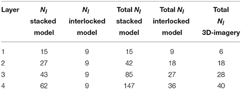
Table 2. Comparison of the number of coccoliths, N_l, attached to a coccosphere of radius 3.7 μm for 1–4 layers for stacked and interlocked liths of semi-major axis length 1.7 μm and as observed on 3D imagery of coccospheres by Hoffmann et al. (2015).

The analysis of the ratio of the backscattering cross-section for free liths to that of the coated coccosphere with interlocked liths is similar to that for the stacked liths model. The total area of the core covered by the liths stays the same for all layers and therefore the total lith area is:

$\begin{array}{ll}2\pi r_c^2\left(1-f_t^2\right)O_{vl}& (51)\end{array}$

We thus find the following ratio for a non-absorbing core:

$\begin{array}{ll}\frac{{\sigma }_{bbNl}}{{\sigma }_{bbs}}=\frac{Q_{bbl}2\pi r_c^2\left(1-f_t^2\right)O_{vl}\left(1+\frac{\left(1+r\right)}{2r}{f}_d\right)}{Q_{bbl}2\pi r_c^2\left(1-f_t^2\right)O_{vl}}=1+\frac{\left(1+r\right)}{2r}{f}_d& (52)\end{array}$

which is exactly the same as for the stacked liths model given in Equation (40). For an absorbing core, we also find the same ratio as for the stacked liths model:

$\begin{array}{ll}\frac{{\sigma }_{bbNl}}{{\sigma }_{bbs}}=\frac{2\left(1+\frac{\left(1+r\right)}{2r}{f}_d\right)}{\left[2-Q_{as}\left(k,2r_c\right)\frac{1}{{\left(1+O_{vl}\frac{\Delta r_s}{r_c}\right)}^2}\right]}& (53)\end{array}$

Only the absolute magnitudes of the cross-sections between both models are different since for the first layer we have:

$r_s^2={\left(r_c+\Delta r_s\right)}^2$

Based on the coccolithophore structure measured by Hoffmann et al. (2015), the lith morphology obtained by Young et al. (2014), and our previous results we determine the following general values for the key parameters in Equation (53):

$f_d=\frac{1}{4},\frac{\Delta r_s}{r_c}=\frac{1}{5},r=1.2$

In summary, no matter which coccosphere architecture model we use, we get the fundamental result that backscattering from detached coccoliths is not so much greater than the backscattering from the coccolithophore with its coccoliths attached, which confirms the suggestion of Gordon et al. (2009), and that the difference in backscattering is governed by the absorption of the core which has a spectral signature.

Changes in Light Backscattering and Remote Sensing Reflectance During E. Huxleyi Bloom Decay

We simulate changes in spectral backscattering during a hypothetical E. huxleyi bloom decay phase in which E. huxleyi sheds all its attached liths. We will account for two possibilities for the fate of the E. huxleyi cores; they either die during bloom decay (for example due to viral lysis), or they remain without liths (Balch et al., 1993). Their presence only affects light absorption (and by consequence remote sensing reflectance) as we assume that the calcite material dominates the backscattering coefficient, in agreement with observations in natural E. huxleyi blooms. These bloom dynamics scenarios are based on observations of bloom decay in laboratory experiments and in situ (Balch et al., 1993) with the following simplifications: (i) coccolith production stops when shedding begins so that the number of liths remains constant during the process and none are detached at the beginning, and (ii) dead E. huxleyi cores do not absorb light and the light absorption properties of the cores that remain without liths remain constant throughout the bloom event. Thus, initially we have a suspension of living E. huxleyi cells, coccospheres with absorbing cores and with all N_ltot liths attached. This suspension then gradually transforms into a suspension comprised of free liths with a certain fraction of surviving absorbing cores left, F_sc, which varies between 0 and 1.

If we define F_nc as the ratio of cores that have shed their liths to the total initial number of coated cores (F_nc = number of naked cores/N_cc), which varies from 0 to 1 during the coccolith shedding event, we can express the total backscattering cross-section σ_bbtot at any given point during the event as follows:

$\begin{array}{ll}{\sigma }_{bbtot}=F_{nc}{\sigma }_{bbNl}+\left(1-F_{nc}\right){\sigma }_{bbs}& (54)\end{array}$

with

$\begin{array}{ll}{\sigma }_{bbNl}=Q_{bbl}2\pi r_c^2\left(1-f_t^2\right)O_{vl}\left(1+\frac{\left(1+r\right)}{2r}{f}_d\right)& (55)\end{array}$

the backscattering cross-section of the free liths when detached from a single coccolithophore, and

$\begin{array}{ll}{\sigma }_{bbs}={\sigma }_{bbNl}\frac{\left[2-Q_{as}\left(k,2r_c\right)\frac{1}{{\left(1+O_{vl}\frac{\Delta r_s}{r_c}\right)}^2}\right]}{2\left(1+\frac{\left(1+r\right)}{2r}{f}_d\right)}& (56)\end{array}$

$\begin{array}{ll}{\sigma }_{bbs}=Q_{bbl}\pi r_c^2\left(1-f_t^2\right)O_{vl}\left[2-Q_{as}\left(k,2r_c\right)\frac{1}{{\left(1+O_{vl}\frac{\Delta r_s}{r_c}\right)}^2}\right]& (57)\end{array}$

the backscattering cross-section of a coated coccolithophore.

Algebraic Radiance Model

To evaluate variability in ocean color remote sensing due to changes in the size distribution of E. huxleyi coccoliths and during bloom decay, we develop an algebraic remote sensing reflectance model. The model is based on the work of Albert and Mobley (2003), which provides a polynomial parameterization of the deep water reflectance R_rs∞(λ) (units: sr⁻¹) in terms of the dimensionless backscattering albedo x(λ):

$\begin{array}{ll}\begin{array}{l}{R}_{rs\infty }(\lambda )=p_{1}x(\lambda )(1+p_{2}x(\lambda )+p_{3}x{(\lambda )}^2\\ +p_{4}x{(\lambda )}^3)\left(1+p_5\frac{1}{\cos {\theta }_s}\right)\left(1+p_7\frac{1}{\cos {\theta }_v}\right)\left(1+p_{6}u\right)\end{array}& (58)\end{array}$

with coefficients p₁ = 0.0512 sr⁻¹, p₂ = 4.6659 sr⁻¹, p₃ = −7.8387 sr⁻¹, p₄ = 5.4571 sr⁻¹, p₅ = 0.1098 sr⁻¹, p₆ = −0.0044 s m⁻¹, and p₇ = 0.4021 sr⁻¹. θ_s is the zenith angle of the sun under the water surface and θ_v is the sensor viewing angle also below the water surface, and u is the mean wind speed. We used a mean value over the world's oceans of u = 6.9 m s⁻¹, θ_s = 29°, typical for summer at temperate latitudes (40–60°N). The model is valid even in turbid water with large backscattering albedo, which is given by:

$\begin{array}{ll}x(\lambda )=\frac{b_b(\lambda )}{b_b(\lambda )+a(\lambda )}& (59)\end{array}$

with total absorption coefficient, a(λ)(in m⁻¹), composed as follows

$\begin{array}{ll}a(\lambda )=a_w(\lambda )+a_{cc}(\lambda )+a_{cdom}(\lambda )+a_{ph}(\lambda )& (60)\end{array}$

where a_w(λ), a_cc(λ), a_cdom(λ), and a_ph(λ) are the respective contributions from pure seawater, coccolithophore cores, colored dissolved organic matter (CDOM), and phytoplankton other than coccolithophores. To focus on the effect of coccolithophores, we assumed a_w(λ), a_cdom(λ), and a_ph(λ) to be constant. We fixed the chlorophyll-a concentration from other phytoplankton to a value of 0.6 mg m⁻³ and set a_cdom = 0.02 at a wavelength of 0.443 μm with a spectral slope of 0.0172 nm⁻¹, corresponding to average values for the Atlantic (Babin et al., 2003). See Supplementary Materials for more details on the calculation of a(λ).

The total backscattering coefficient b_b(λ) is partitioned as follows:

$\begin{array}{ll}{b}_b(\lambda )=b_{bw}(\lambda )+b_{bpic}(\lambda )& (61)\end{array}$

where b_bw(λ)is the backscattering coefficient of pure water and b_bpic(λ) is the backscattering coefficient of the coccolith-coccosphere mixture as in Equation (1). We note that we have assumed negligible contribution to backscattering from the organic part of the coccolithophore as the refractive index of the organic part of the coccolithophore is estimated to be 1.06 relative to water (Aas, 1996), much smaller than the refractive index of its calcite coccosphere, which is 1.20 relative to water. Further details of the model can be found in Supplementary Information section 1.3.

As derived in Supplementary Information section 1.3, the coccolith core absorption term is given by

$\begin{array}{ll}{a}_{cc}(\lambda )=N_{cc}{a}_{cc}^{*}(\lambda )& (62)\end{array}$

where N_cc is the number concentration of coccospheres (in m⁻³) and $a_{cc}^{*}(\lambda )$ is the coccosphere-specific absorption coefficient (in m⁻² per coccosphere) resulting from an integral over the size distribution of the cores:

$\begin{array}{ll}{a}_{cc}^{*}(\lambda )=\underset{0}{\stackrel{\infty }{\int }}P\left(\mu ,\sigma ,a_0\right)Q_a\left(k,r_c\right)\pi r_c^{2}d{a}_0& (63)\end{array}$

We note that if we neglect the backscatter loss from the front surfaces which we can do to first order, the absorption by the cores is independent of whether they are coated or not. We can thus write:

$\begin{array}{ll}{a}_{cc}(\lambda )=N_{cc}\left[F_{sc}{F}_{nc}+\left(1-F_{nc}\right)\right]a_{cc}^{*}(\lambda )& (64)\end{array}$

where F_nc is the proportion of naked cores and F_sc is the fraction of naked cores that remain in the surface after their liths have been shed (F_sc = number of surviving naked cores /N_cc). The first term represents the absorption from the naked cores left in the surface layer after lith shedding, while the second term represents the absorption from the coated cores in the bloom.

The backscattering term results from Equation (54):

$\begin{array}{ll}{b}_{bpic}(\lambda )=N_{cc}\left[\left(1-F_{nc}\right){\sigma }_{bbs}(\lambda )+F_{nc}{\sigma }_{bbNl}(\lambda )\right]& (65)\end{array}$

Even though cell densities in bloom conditions for E. huxleyi are somewhat arbitrary, a minimal value of 10⁹ cells m⁻³ has been suggested (Tyrrell and Merico, 2004), with cell concentration exceeding 10¹¹ cells m⁻³ in the most intense blooms observed in Norwegian fjords (Tyrrell and Merico, 2004). Therefore, a realistic range for initial coccolithophore concentrations would be between N_cc = 10⁹ and 2 × 10¹⁰ cells m⁻³ in open ocean waters, which we will use to simulate changes in remote sensing reflectance.

Results

Spectral Backscattering Efficiency for a Single Coccolith as a Function of Size, Shape, and Morphology

The refractive index of calcite does not vary significantly over the wavelength range and can be represented by an average value of 1.2, which gives ω_brg and ω_bsm (Fournier and Neukermans, 2017), so that Q_bbl is only a function of λ_w/a_o, as shown in Figure 4. For a coccolith with semi-major axis length a_o, in the long wavelength limit the entire surface of the particle appears perfectly smooth since asperities or holes will be smaller than λ_w/4, and Q_bbl = ω_bsm(1 − RF_rg). As the wavelength gets shorter, parts of the surface will start to appear as rough and Q_bbl will increase rapidly to reach a maximum value of Q_bbl = ω_brgF_rg + ω_bsm(1 − F_rg) when all asperities and holes are larger than λ/4. This is very similar to the result obtained when modeling circular coccoliths with the morphology described by Zhai et al. (2013).

FIGURE 4

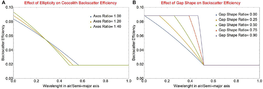
Figure 4. Backscattering efficiency factor Q_bbl vs. the ratio of wavelength in air to the length of the semi-major axis of a coccolith a_o for (A) various values of the aspect ratio r₀ = a_o/b_o of the elliptical coccolith, and (B) various values of the gap shape factor r_sh = Δs_gmin/Δs_gmax.

The backscattering efficiency for an elliptical coccolith with various aspect ratios r₀ = a_o/b_o is shown in Figure 4A. The change seen in the onset wavelength is due to the reduction in the maximum gap width as the overall perimeter of the lith is reduced because the axis ratio increases. The accompanying change in the maximum value of the backscattering efficiency is due to the increase in the maximum fraction F_rg of rough area to total area because of the increasingly elliptical shape. The effect of the gap shape factor r_sh (defined in Equation 9) is shown in Figure 4B for an elliptical axis ratio r₀ of 1.2. This factor is a significant determinant of the spectral shape of light backscattering. In the limiting case of a constant gap width (r_sh ≈ 1) the complete change from smooth to rough backscatter will occur in a very narrow wavelength range. As the wedge gap narrows to a triangular shape (r_sh ≈ 0) the change will become more gradual. As this triangular shape is the one observed by Young et al. (2014), we will use it in the rest of this paper.

Spectral Backscattering Efficiency for Populations of Elliptical Coccoliths

Figure 5 shows the spectral shape of backscattering efficiency for various coccolith size distributions modeled as a second order shifted Gamma function with five different mean semi-major axes μ and five standard deviations σ as defined in Equation (27). Not surprisingly, the sharp spectral features observed for a single coccolith particle in Figure 4 are smoothened when averaged over the size distribution. Figure 5 shows that the spectral shape of backscattering is largely controlled by variations in mean size of the coccolith population, whereas the standard deviation is a secondary factor merely broadening the transition zone from smooth to rough scattering as the standard deviation increases.

FIGURE 5

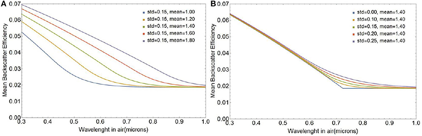
Figure 5. Average backscattering efficiency for a second order shifted Gamma distribution of liths as a function of mean a₀ for a standard deviation of 0.15 (A) and as a function of standard deviation for a mean a₀ of 1.4 μm (B).

Differences in 〈σ_bbl(λ)〉 between the first order gamma function used in our original work the second-order gamma models for coccolith size distributions are very small because the Gamma functions have the same mean and standard deviation. However, in what follows, we will use the second-order Gamma function to represent the coccolith size distribution as it matches the experimental size distributions more closely (see Supplementary Information section 1.2).

The changes in the spectral shape of light backscattering efficiency as the mean lith size changes are due to the fact that the transition from smooth to rough backscattering occurs at longer wavelengths as the size of the gap increases, which corresponds to an increase in coccolith size for a fixed coccolith morphology. The effect is shown in Figure 5A for a change in mean coccolith major axis of 2.0 to 3.6 μm, which corresponds to the range observed in the lab and the field.

Differences in Spectral Light Backscattering Between Free and Attached Coccoliths

Figure 6A depicts variations in the spectral behavior of the ratio σ_bbNl/σ_bbs for a coccolithophore with a single layer of liths and core radius r_c ranging between 2.75 and 3.2 μm which matches the ranges observed by Young et al. (2014). At wavelengths shorter than 0.5 μm, backscattering from free liths is 40–60% higher than backscattering from coated spheres and about 30% higher at larger wavelengths. Increasing the number of coccolith layers reduces the region where the core is absorbing and leads to smaller differences in backscattering cross-section between free and attached liths as can be seen in Figure 6B. We used a core radius of 3.0 μm which corresponds to a mean lith major axis value of 3.3 μm (Zhai et al., 2013), close to those measured by Young et al. (2014). For four layers of coccoliths, the total number of coccoliths on the coccosphere is 40. For that many layers the coated coccolithophores are nearly spectrally indistinguishable from the free liths and backscattering from free liths is at most 35% higher than backscattering from coated spheres.

FIGURE 6

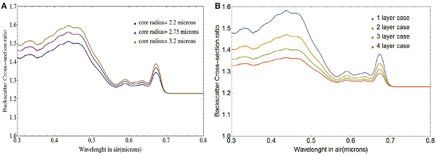
Figure 6. Ratio of free coccolith to coated coccolithophore backscattering cross-section σ_bbNl/σ_bbs, for (A) single-layer coated coccospheres of varying core radii and (B) coccospheres with varying number of coccolith layers and a core radius of 3.0 μm.

Note that for a single layer of interlocked liths the first surface could simply be completely covered. If there are multiple layers however, all the layers must have about the same number of coccoliths per layer. The interlocked liths model leads to substantially smaller number of liths for a given number of layers and reduces further the difference between the backscattering from the sum of the free coccoliths and from the fully coated coccolithophore cores.

Changes in Spectral Light Backscattering During E. huxleyi Coccolith Shedding Event

Figure 7 shows changes in the magnitude and spectral shape of the backscattering cross section σ_bbtot(λ) for a coccolithophore with a core radius of 3.7 μm, shedding four layers of liths with mean a_o of 1.7 μm and standard deviation of 0.15 μm, obtained through integration of expressions in Equations (55) and (57). Note that the particulate backscattering coefficient b_bp (λ) can be obtained by multiplication of σ_bbtot (λ) with the initial number concentration of coated cores, N_cc. The size of the coccosphere (which also fixes the size of the liths) and number of coccolith layers chosen for this simulation corresponds to a coating of the coccosphere with 36 liths (Table 1). This gives a coccolith-to-cell ratio of 36, on the lower range of what has been observed for coccolith-to-cell ratios in natural and laboratory E. huxleyi blooms, which vary between 45 and 400 liths per cell (e.g., Balch et al., 1991, 1993; Gordon et al., 2009). Potential causes for a lower coccolith-to-cell ratio than observed in laboratory experiments and in the field are: (i) E. huxleyi's continued calcification during the coccolith shedding phase, (ii) the presence of detached coccoliths before the shedding begins (Balch et al., 1993), and (iii) the preferential sinking of coccospheres out of the surface layer due to their larger size, but see Monteiro et al. (2016).

FIGURE 7

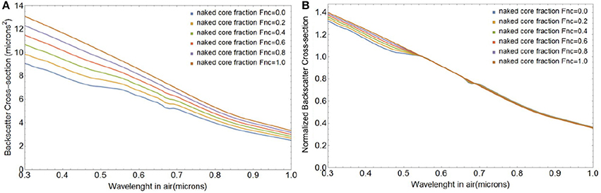
Figure 7. Changes in the total spectral backscattering cross-section σ_bbtot magnitude (A) and spectral shape (B) as a coccolithophore with a core radius r_c of 3.7 μm, a lith semi-major axis a₀ of 1.7 μm, and 4 layers of liths sheds its liths.

The spectral shape of b_bp(λ) is commonly described by the relationship (Gordon and Morel, 1983):

$\begin{array}{ll}{b}_{bp}(\lambda )=b_{bp}\left({\lambda }_0\right){(\lambda /{\lambda }_0)}^{\xi }& (66)\end{array}$

where λ_o is a reference wavelength and ξ represents the dimensionless spectral slope parameter of b_bp(λ). Calculated over the 0.4–0.7 μm wavelength range, ξ changes from −0.77 to −0.94 for coated spheres to free liths (Figure 7B). Even though not strictly quantitatively comparable, our results are consistent with multispectral b_bp(λ) measurements in E. huxelyi cultures who reported a steepening of the spectral slope of b_bp(λ) for suspensions of free liths compared to coccospheres (Voss et al., 1998), from ξ = −1.2 to ξ = −1.4. We note that the experimental error on the slopes calculated by Voss et al. (1998) were large and that the morphology of E. huxelyi was not determined. A change to the shape or size of the openings will lead to a change of slope as shown in Figure 4 for a single lith.

Ocean Color Remote Sensing Reflectance for E. Huxleyi Populations of Different Size Distribution and Bloom Stage

Implementing our optical model for light backscattering from E. huxleyi coccoliths and coccospheres into the analytical radiance model presented in section Algebraic Radiance Model, we can investigate the variability in ocean color remote sensing reflectance for blooms of different magnitudes, with different lith size distributions, and during different stages.

The variability in magnitude and spectral shape of the above-water remote sensing reflectance R_rs(λ) (in sr⁻¹) during a lith shedding event of E. huxleyi blooms with initial coccolithophore concentrations ranging between N_cc = 10⁹ and 2 × 10¹⁰ cells m⁻³ is depicted in Figure 8. We assumed a coccolith size distribution with a mean a₀ of 1.7 μm and standard deviation of 0.15 μm and coccospheres with four layers of liths, totaling 36 coccoliths per coccosphere for all our simulations, unless noted otherwise. Figures 8A,B shows the magnitude and spectral shape of R_rs(λ) at the initial stage with all liths attached (F_nc = 0) and Figures 8C,D shows the final stage with all liths shed (F_nc = 1) and no living cores remaining (F_sc = 0). Before the onset of lith shedding, the absorption features of the cores clearly influence R_rs(λ) by reducing reflectance in blue wavelengths (~ 0.4 − 0.47 μm), resulting in peak R_rs(λ) at green wavelengths (~ 0.50 − 0.55 μm). When the liths are freed and no cores are left to absorb light, R_rs(λ) increases by a factor of up to four and the peak in R_rs(λ) shifts toward blue-turquoise wavelengths (~ 0.40 − 0.49 μm), where R_rs(λ) shows little spectral variation. This gives a bright milky turquoise coloring of the ocean, typically associated with E. huxleyi blooms. Our modeled R_rs(λ) spectra are also quantitatively consistent with multispectral ocean color satellite observations of R_rs(λ) in coccolithophore blooms which have been shown to peak at 0.49 μm (Moore et al., 2012).

FIGURE 8

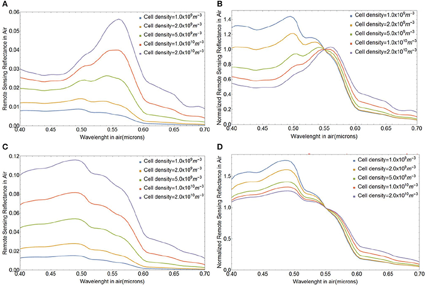
Figure 8. Variability in the spectral remote sensing reflectance R_rs(λ) (in sr⁻¹) during coccolith shedding by E. huxleyi in blooms with various initial coccolithophore concentrations and for a coccolith size distribution with a mean a₀ of 1.7 μm and standard deviation of 0.15 μm and coccospheres with four layers of liths. (A) Initial stage with all liths attached (F_nc = 0), (C) final stage with all liths shed (F_nc = 1) and no living cores remaining (F_sc = 0). Spectra in (B,D) were normalized at a wavelength of 0.55 μm. Note that the lith concentration in panels (C,D) is simply 36 times the cell density.

Next we investigate the influence of changes in the fraction of naked cores (F_nc) or surviving cores (F_sc) on R_rs(λ) during different stages of a bloom with initial E. huxleyi coccolithophore concentration of 10⁹ cells m⁻³. Figures 9A,B shows how R_rs(λ) changes when the coated cores shed their liths and they die after shedding, i.e., F_sc = 0. Even though there are significant changes in the magnitude of R_rs(λ), the spectral variability is clearly small, and appears to be too small to be detectable from satellite ocean color observations which typically have uncertainties around 5% at visible wavelengths. The change in spectral shape of R_rs(λ) due to lith shedding will, however, be more pronounced for larger cell concentrations. Figures 9C,D illustrates variability in R_rs(λ) due to changes in the fraction of cores that remain in the surface after lith shedding (F_sc from 0 to 1 when F_nc = 1). Such changes result in much stronger spectral variability in R_rs(λ) by virtue of their absorption features (Figures 9C,D).

FIGURE 9

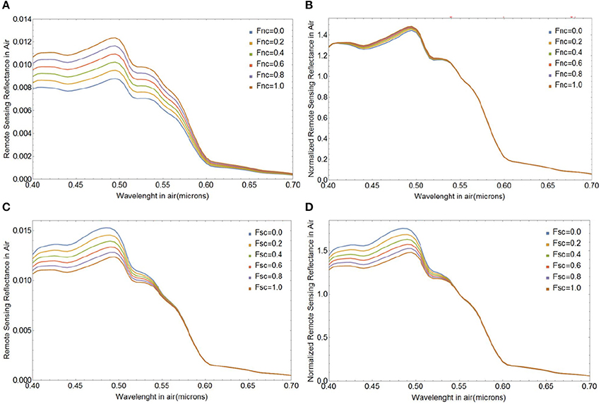
Figure 9. Spectral above-water remote sensing reflectance R_rs(λ) in absolute values of sr⁻¹ (A,C) and normalized at 0.55 μm (B,D) for various fractions of naked cores (F_nc = 0 to 1, top row), and various surviving core fractions (F_sc = 0 to 1, bottom row). We used a size distribution of free liths of mean a₀ 1.7 μm and standard deviation of 0.15 μm, an initial coccolithophore cell concentration of 10⁹ m⁻³ and four layers of liths.

Lastly, Figure 10 illustrates how changes in the mean size of free liths impact the magnitude and spectral shape of R_rs(λ). The magnitude of R_rs(λ) increases with increasing mean size mostly due to increases in the geometric cross section. The spectral shape of R_rs(λ) varies significantly over the wavelength range considered: smaller-sized coccoliths produce stronger relative reflection at shorter wavelengths, which offers the potential for ocean color remote sensing of coccolith size distribution.

FIGURE 10

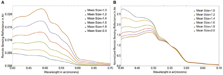
Figure 10. (A) Absolute and (B) normalized spectral remote sensing reflectance R_rs(λ) (in sr⁻¹) for populations of free coccoliths of varying mean size, a₀. The standard deviation of the size distribution was 0.15 μm.

Discussion

Our model results indicate that light backscattering from detached E. huxleyi coccoliths is at most twice as large as the backscattering from the same liths when arranged in a coccosphere. This result is consistent with the suggestion of Gordon et al. (2009), but may come as a surprise as it has been commonly assumed that the backscattering from coccoliths would be orders of magnitude higher than for coccospheres. The implication of this result is that the calcite-specific backscattering coefficient, b_bp/PIC, for E. huxleyi coccoliths of a given size and morphology varies by at most a factor of two between coated cores and free liths. For E. huxleyi coccolith populations of a given size and morphology, light backscattering is thus a good proxy for calcite mass concentration, regardless of whether coccoliths are attached to or freed from the core. The difference between scattering from free and attached liths is smallest in regions of the spectrum where absorption of the core is minimal, i.e., between 0.54 and 0.66 μm and wavelengths larger than 0.7 μm. Another implication is that the order of magnitude increase in backscattering frequently observed at the final bloom stages is likely mostly due to the excess production of coccoliths and only a small part of this increase is due to the shedding of the attached liths.

We have demonstrated that the magnitude and spectral shape of light backscattering by coccoliths are strongly sensitive to coccolith size and morphology, which suggests that information on the size and morphology are potentially amenable from hyperspectral backscattering measurements. In what follows, we describe a potential avenue for estimating coccolith size from b_bp(λ). The spectral shape of b_bp(λ) from a single coccolith is characterized by the onset of a sharp increase at a definite wavelength due to a transition from smooth to rough scattering. This onset wavelength in air, λ_onset, is determined by the gap width at the outer perimeter from Equation (10) as follows:

$\begin{array}{l}{\lambda }_{onset}=n_{w}4\Delta s_{gmax}=n_{w}4\frac{2\pi a_0{P}_n\left(\frac{a_r}{a_o},\frac{b_r}{a_o}\right)}{N\left(1+r_{pg}\right)},\\ Q_{bbl}\left({\lambda }_{onset}\right)={\omega }_{bsm}& (67)\end{array}$

where N is the number of gaps, r_pg is the pillar to gap ratio defined in Equation (9), n_w is the refractive index of seawater, and P_n is the non-dimensional form of the perimeter of the lith defined in Equation (S13). For a given lith morphology, which fixes the values of N, r_pg, a_r/a_o, and b_r/b_o, the lith size a₀ can thus be estimated. Equation (67) expresses the condition that at the transition from smooth to rough backscattering, the gap width is equal to a quarter of the wavelength in water. As the wavelength gets shorter the backscattering efficiency increases from a value of ω_bsm to a maximum value of:

$\begin{array}{ll}{Q}_{bbl}\left(\lambda \to 0\right)={\omega }_{brg}{F}_{rg}+{\omega }_{bsm}\left(1-F_{rg}\right)& (68)\end{array}$

where F_rg is the fraction of the surface of the lith which is composed of gaps and pillars and which obviously depends on the assumed morphology (see Equation 7), and ω_brg and ω_bsm are respectively the rough and smooth reflectivities of the lith surfaces and only depend on the index of refraction of the calcite material of the lith, which is 1.2.

In the simple case of a population of coccoliths of fixed morphology, the parameters that directly control the spectral shape of b_bp(λ) are and F_rg. Our results suggest that the mean lith size of the population may be obtained from the spectral shape of b_bp(λ) assuming a functional form for the size distribution of liths expressed in terms of a mean particle size μ and standard deviation σ. To help solve for the size distribution parameters, it would be advantageous if a relationship between μ and σ could be established. From proportionality arguments one would expect a linear relationship to apply to first order. Such a fit applied to the data of Young et al. (2014) gives σ ≈ 0.11μ . However, because of the small range of sizes and the significant spread of σ the R² coefficient of determination is only 0.25. More particle size distribution measurements over larger size ranges will be needed to improve solving for mean population size.

All the above relies on an assumed lith morphology, which is known to vary among morphotypes of E. huxleyi (Young et al., 2003; Cook et al., 2011; Hagino et al., 2011). The coccolith morphology and size range assumed in this paper are based on the work of Young et al. (2014) for E. huxleyi of morphotype A. Optical models for different morphotypes of E. huxleyi could be set up for example by adjusting the proportionalities in Equations (6) and (9). The corresponding inversion algorithms to estimate lith size from b_bp(λ) would thus also be morphotype-specific. Of primary importance in these efforts is the relationship between the gap width and the lith size, as this forms the basis of the size estimation. As pointed out earlier, an assessment of the relationships between statistical parameters of the size distribution, such as the standard deviation and mean, would also be desirable.

Our model further illustrates that when a population of E. huxleyi sheds its liths, the spectral shape and magnitude of b_bp(λ) change surprisingly little. This is due to the quasi-equality of the backscattering cross-sections of the same amount of liths when free or arranged in a coccosphere. The subtle changes in b_bp(λ) are due to the increase in backscattering by the free liths that are no longer obscured by the core absorption. Nevertheless, our results suggest that estimation of the fraction of cores that have shed their liths (F_nc) appears to be feasible if accurate measurements of the spectral slope of b_bp (λ) can be obtained. This information may be exploited to develop approaches to determine the proportional contribution of coccoliths and coccolithophores to total calcite, which may be of interest in biogeochemical and ecological studies of coccolithophores. While coccolithophores are marine microalgae which contribute to primary production, calcification (Monteiro et al., 2016), and the production of dimethylsulfoniopropionate (Matrai and Keller, 1993), coccoliths are dead material thought to enhance the flux of organic carbon to the deep ocean by providing ballast material (Armstrong et al., 2001; Riebesell et al., 2016).

We have also modeled the remote sensing reflectance R_rs(λ) during various stages of hypothetical E. huxleyi blooms in which coccoliths are shed and the naked cores either die or survive. This allows us to investigate which characteristics of E. huxleyi bloom state are potentially resolvable from hyperspectral ocean color remote sensing. As expected from the subtlety of changes in spectral b_bp(λ) when coccolithophores shed their liths and naked cores die, changes in spectral R_rs(λ) are similarly small and therefore unlikely to be detectable from space. In a population of free liths at the end of a shedding event, the fraction of surviving cores had a much more pronounced effect on R_rs(λ) by virtue of their absorption. However, similar effects on R_rs (λ) can be expected from changes in the absorption of phytoplankton other than coccolithophores, which is assumed constant in our simulations. Therefore, the potential to estimate naked E. huxleyi cells depends on how different their absorption features are from other types of phytoplankton.

Our modeled R_rs(λ) were produced assuming a constant background of absorption by CDOM and chlorophyll-a from phytoplankton other than E. huxleyi, as well as negligible contribution to backscattering from particles other than E. huxleyi coccoliths and coccospheres. This is obviously an overly simplified representation of real bloom conditions. The assumption of constant non-zero CDOM absorption was essential to obtain the spectral shape of R_rs (λ) typically associated with E. huxleyi blooms, i.e., one that produces a turquoise hue with peak reflectance at 0.49 μm (Moore et al., 2012). This is because CDOM absorbs strongly in violet-blue wavelengths. If CDOM absorption is not included in the background, R_rs(λ) would peak at violet wavelengths and the magnitude of R_rs(λ) would be much more intense than observed from ocean color satellites and in the field. The impact of CDOM absorption on reflectance from a suspension of 3.6 × 10¹⁰ m⁻³ free coccoliths and no absorption due to chlorophyll-a is demonstrated in Figure 11A, whereas Figure 11B also includes the absorption effect of 10⁹ m⁻³ E. huxleyi cores.

FIGURE 11

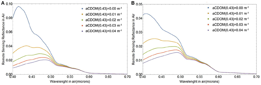
Figure 11. Spectral remote sensing reflectance R_rs(λ) (in sr⁻¹) from the free liths shed by N_cc = 10⁹ E. huxleyi cells m⁻³ in waters with a_ph(λ) = 0 and varying CDOM absorption, when (A) all cores have died, F_sc = 0 and when (B) all cores survived, F_sc = 1. The coccolith size distribution had a mean of 1.7 μm and standard deviation of 0.15 μm and the coccospheres were coated with four layers of liths.

In coccolithophore blooms characterized by high concentrations of PIC (>0.003 mol C m⁻³) the ocean color remote sensing algorithm of Gordon et al. (2001) is used to derive PIC. Because bands at shorter wavelengths often saturate in these bloom conditions, the algorithm uses R_rs(λ) in three bands in the red and near-infrared (0.670, 0.765, and 0.865 μm) to estimate b_b from R_rs at 0.670 μm assuming R_rs = 0 in the 0.765 and 0.865 μm bands to perform the aerosol scattering correction. From the range of coccolith concentrations used in Figure 8C we find R_rs at 0.765 and 0.865 μm much lower than R_rs at 0.670 μm, thereby providing support for the atmospheric correction approach of Gordon et al. (2001). We suggest that our model may be used to improve on the atmospheric correction approach of Gordon et al. (2001).

We have assumed throughout this work that the detached coccoliths are randomly oriented with respect to incident light, which allows us to apply the theorem of Cauchy (1850) to calculate the average geometric cross-section via Equation 3. However, it has recently been shown that large phytoplankton cells and marine aggregates have a tendency to orient horizontally in natural waters (Nayak et al., 2018). If coccoliths, even though much smaller in size, have just a slight tendency to orient horizontally with respect to incident light, the influence on backscattering will be significant, because light is scattered off a larger surface. As a consequence the difference in backscattering between oriented coccoliths and coccolithophores will be much larger. We can estimate the limits of this effect by taking the ratio of the randomly oriented liths surface to the surface at normal incidence.

$\begin{array}{ll}{R}_{ori}\approx \frac{\pi ab}{\left[\frac{2\pi ab+2\pi \left(a+b\right){\tau }_l}{4}\right]}=\frac{2}{1+\left(1+r\right)\left(\frac{{\tau }_l}{a}\right)}& (69)\end{array}$

For completely oriented very thin liths the cross-section is therefore approximately twice that of randomly oriented liths. To distinguish this orientation effect in natural waters, new observational approaches such as circular polarization will be needed to study preferential particle orientation.

Besides the assumption of random orientation of the coccoliths and coccolithophores, our approach is also based on the assumption that the unity-normalized angular distribution of reflection from any randomly oriented convex body is independent of shape and size (van de Hulst, 1957), implicit in Equation (3). When backscattering is dominated by reflection, such as for high refractive index coccoliths and coccolithophores, this implies that the scattering efficiency Q_bb is independent of shape and size and only dependent on the relative amount of rough and smooth surfaces comprising the particle. This angular constancy is the physical underpinning of our analytical light backscattering model and also allows us to carry out the averaging of Q_bb over a size distribution. The fact that our modeled backscattering cross-sections for circular disk-like coccoliths compared successfully with exact scattering solutions from the discrete dipole approximation (Fournier and Neukermans, 2017) provides general support to our assumptions. We expect the validity of the angular constancy assumption to break down as the particle shapes become more complex and self-shadowing (non-convexity) becomes significant, which can be investigated using exact light scattering codes such as discrete dipole approximation, T-Matrix, or Finite Difference Time Domain (FDTD) approaches (e.g., Gordon and Du, 2001; Hedley, 2012; Zhai et al., 2013).

A thorough validation of our light scattering model for E. huxleyi requires simultaneous measurements of E. huxleyi coccolith morphology, size distribution, and spectral light backscattering, which can be obtained in laboratory cultures. Further validation work will also entail conjunct in situ observations of (hyperspectral) remote sensing reflectance, inherent optical properties, E. huxleyi coccoliths and coccolithophore size distribution and morphology, and characterization of other optically active constituents during E. huxleyi blooms. Such measurements in the laboratory and in natural waters are essential to the evaluation of the current model and will inform on potential modeling improvements.

Author Contributions

GN and GF conceptualized the study; GF developed the model. Both authors discussed results and wrote the manuscript.

Funding

GN is supported by a European Union's Horizon 2020 Marie Sklodowska-Curie grant (no. 749949).

Conflict of Interest Statement

The authors declare that the research was conducted in the absence of any commercial or financial relationships that could be construed as a potential conflict of interest.

Acknowledgments

We would like to thank Dariusz Stramski and Aimee Neeley for providing the spectral absorption coefficient for an Emiliania huxleyi culture.

Supplementary Material

The Supplementary Material for this article can be found online at: https://www.frontiersin.org/articles/10.3389/fmars.2018.00146/full#supplementary-material

References

Aas, E. (1996). Refractive index of phytoplankton derived from its metabolite composition. J. Plankton Res. 18, 2223–2249. doi: 10.1093/plankt/18.12.2223

CrossRef Full Text | Google Scholar

Albert, A., and Mobley, C. (2003). An analytical model for subsurface irradiance and remote sensing reflectance in deep and shallow case-2 waters. Opt. Exp. 11:2873. doi: 10.1364/OE.11.002873

PubMed Abstract | CrossRef Full Text | Google Scholar

Armstrong, R. A., Lee, C., Hedges, J. I., Honjo, S., and Wakeham, S. G. (2001). A new, mechanistic model for organic carbon fluxes in the ocean based on the quantitative association of POC with ballast minerals. Deep Sea Res. Part II Top. Stud. Oceanogr. 49, 219–236. doi: 10.1016/S0967-0645(01)00101-1

CrossRef Full Text | Google Scholar

Babin, M., Stramski, D., Ferrari, G. M., Claustre, H., Bricaud, A., Obolensky, G., et al. (2003). Variations in the light absorption coefficients of phytoplankton, nonalgal particles, and dissolved organic matter in coastal waters around Europe. J. Geophys. Res. 108:3211. doi: 10.1029/2001JC000882

CrossRef Full Text | Google Scholar

Balch, W. M., Drapeau, D. T., Bowler, B. C., Lyczskowski, E., Booth, E. S., and Alley, D. (2011). The contribution of coccolithophores to the optical and inorganic carbon budgets during the southern ocean gas exchange experiment: new evidence in support of the “great calcite belt” hypothesis. J. Geophys. Res. 116:C00F06. doi: 10.1029/2011JC006941

CrossRef Full Text | Google Scholar

Balch, W. M., Gordon, H. R., Bowler, B. C., Drapeau, D. T., and Booth, E. S. (2005). Calcium carbonate measurements in the surface global ocean based on moderate-resolution imaging spectroradiometer data. J. Geophys. Res. 110:C07001. doi: 10.1029/2004JC002560

CrossRef Full Text | Google Scholar

Balch, W. M., Holligan, P. M., Ackleson, S. G., and Voss, K. J. (1991). Biological and optical properties of mesoscale coccolithophore blooms in the Gulf of Maine. Limnol. Oceanogr. 36, 629–643. doi: 10.4319/lo.1991.36.4.0629

CrossRef Full Text | Google Scholar

Balch, W. M., Kilpatrick, K. A., Holligan, P., Harbour, D., and Fernandez, E. (1996). The 1991 coccolithophore bloom in the central North Atlantic. 2. Relating optics to coccolith concentration. Limnol. Oceanogr. 41, 1684–1696. doi: 10.4319/lo.1996.41.8.1684

CrossRef Full Text | Google Scholar

Balch, W. M., Kilpatrick, K., Holligan, P. M., and Cucci, T. (1993). Coccolith production and detachment by Emiliania huxleyi (Prymnesiophyceae). J. Phycol. 29, 566–575. doi: 10.1111/j.0022-3646.1993.00566.x

CrossRef Full Text | Google Scholar

Broecker, W., and Clark, E. (2009). Ratio of coccolith CaCO₃ to foraminifera CaCO₃ in late Holocene deep sea sediments. Paleoceanography 24:PA3205. doi: 10.1029/2009PA001731

CrossRef Full Text | Google Scholar

Brown, C. W., and Yoder, J. A. (1994). Coccolithophorid blooms in the global ocean. J. Geophys. Res. 99:7467. doi: 10.1029/93JC02156

CrossRef Full Text | Google Scholar

Cauchy, A.-L. (1850). Mémoire sur la Rectification des Courbes et la Quadrature des Surfaces Courbes. Mémoires l'académie des Sci. tome XXII, 167–177. Available online at: http://gallica.bnf.fr/ark:/12148/bpt6k901828/f173 (Accessed March 26, 2018).

Cook, S. S., Whittock, L., Wright, S. W., and Hallegraeff, G. M. (2011). Photosynthetic pigment and genetic differences between two Southern Ocean morphotypes of Emiliania huxleyi (haptophyta). J. Phycol. 47, 615–626. doi: 10.1111/j.1529-8817.2011.00992.x

PubMed Abstract | CrossRef Full Text | Google Scholar

Fournier, G., and Neukermans, G. (2017). An analytical model for light backscattering by coccoliths and coccospheres of Emiliania huxleyi. Opt. Express 25:14996. doi: 10.1364/OE.25.014996

PubMed Abstract | CrossRef Full Text | Google Scholar

Gordon, H. R. (2006). Backscattering of light from disklike particles: is fine-scale structure or gross morphology more important? Appl. Opt. 45:7166. doi: 10.1364/AO.45.007166

PubMed Abstract | CrossRef Full Text | Google Scholar

Gordon, H. R., Boynton, G. C., Balch, W. M., Groom, S. B., Harbour, D. S., and Smyth, T. J. (2001). Retrieval of coccolithophore calcite concentration from SeaWiFS Imagery. Geophys. Res. Lett. 28, 1587–1590. doi: 10.1029/2000GL012025

CrossRef Full Text | Google Scholar

Gordon, H. R., and Du, T. (2001). Light scattering by nonspherical particles: application to coccoliths detached from Emiliania huxleyi. Limnol. Oceanogr. 46, 1438–1454. doi: 10.4319/lo.2001.46.6.1438

CrossRef Full Text | Google Scholar

Gordon, H. R., and Morel, A. Y. (1983). Remote Assessment of Ocean Color for Interpretation of Satellite Visible Imagery: A Review. Washington, DC: American Geophysical Union.

Google Scholar

Gordon, H. R., Smyth, T. J., Balch, W. M., Boynton, G. C., and Tarran, G. A. (2009). Light scattering by coccoliths detached from Emiliania huxleyi. Appl. Opt. 48:6059. doi: 10.1364/AO.48.006059

PubMed Abstract | CrossRef Full Text | Google Scholar

Groom, S. B., and Holligan, P. M. (1987). Remote sensing of coccolithophore blooms. Adv. Sp. Res 7, 73–78. doi: 10.1016/0273-1177(87)90166-9

CrossRef Full Text | Google Scholar

Hagino, K., Bendif, E. M., Young, J. R., Kogame, K., Probert, I., Takano, Y., et al. (2011). New evidence for morphological and genetic variation in the cosmopolitan coccolithophore Emiliania huxleyi (prymnesiophyceae) from the COX1b-ATP4 genes. J. Phycol. 47, 1164–1176. doi: 10.1111/j.1529-8817.2011.01053.x

PubMed Abstract | CrossRef Full Text | Google Scholar

Hedley, J. (2012). Modelling the optical properties of suspended particulate matter of coral reef environments using the finite difference time domain (FDTD) method. Geo-Mar. Lett. 32, 173–182. doi: 10.1007/s00367-011-0265-8

CrossRef Full Text | Google Scholar

Hoffmann, R., Kirchlechner, C., Langer, G., Wochnik, A. S., Griesshaber, E., Schmahl, W. W., et al. (2015). Insight into Emiliania huxleyi coccospheres by focused ion beam sectioning. Biogeosciences 12, 825–834. doi: 10.5194/bg-12-825-2015

CrossRef Full Text | Google Scholar

Holligan, P. M., Fernández, E., Aiken, J., Balch, W. M., Boyd, P., Burkill, P. H., et al. (1993). A biogeochemical study of the coccolithophore, Emiliania huxleyi, in the North Atlantic. Glob. Biogeochem. Cycles 7, 879–900. doi: 10.1029/93GB01731

CrossRef Full Text | Google Scholar

Hopkins, J., Henson, S. A., Painter, S. C., Tyrrell, T., and Poulton, A. J. (2015). Phenological characteristics of global coccolithophore blooms. Glob. Biogeochem. Cycles 29, 239–253. doi: 10.1002/2014GB004919

CrossRef Full Text | Google Scholar

Iglesias-Rodríguez, M. D., Brown, C. W., Doney, S. C., Kleypas, J., Kolber, D., Kolber, Z., et al. (2002). Representing key phytoplankton functional groups in ocean carbon cycle models: Coccolithophorids. Glob. Biogeochem. Cycles 16, 47-1–47-20. doi: 10.1029/2001GB001454

CrossRef Full Text | Google Scholar

Matrai, P. A., and Keller, M. D. (1993). Dimethylsulfide in a large-scale coccolithophore bloom in the Gulf of Maine. Cont. Shelf Res. 13, 831–843. doi: 10.1016/0278-4343(93)90012-M

CrossRef Full Text | Google Scholar

Monteiro, F. M., Bach, L. T., Brownlee, C., Bown, P., Rickaby, R. E., Poulton, A. J., et al. (2016). Why marine phytoplankton calcify. Sci. Adv. 2:e1501822. doi: 10.1126/sciadv.1501822

PubMed Abstract | CrossRef Full Text | Google Scholar

Moore, T. S., Dowell, M. D., and Franz, B. A. (2012). Detection of coccolithophore blooms in ocean color satellite imagery: a generalized approach for use with multiple sensors. Remote Sens. Environ. 117, 249–263. doi: 10.1016/j.rse.2011.10.001

CrossRef Full Text | Google Scholar

Morel, A., and Bricaud, A. (1981). Theoretical results concerning light absorption in a discrete medium, and application to specific absorption of phytoplankton. Deep Sea Res. Part A. Oceanogr. Res. Pap. 28, 1375–1393. doi: 10.1016/0198-0149(81)90039-X

CrossRef Full Text | Google Scholar

Morel, A., and Bricaud, A. (1986). Inherent optical properties of algal cells, including picoplankton. Theoretical and experimental results. Can. Bull. Fish. Aquat. Sci. 214, 521–559.

Google Scholar

Nayak, A. R., McFarland, M. N., Sullivan, J. M., and Twardowski, M. S. (2018). Evidence for ubiquitous preferential particle orientation in representative oceanic shear flows. Limnol. Oceanogr. 63, 122–143. doi: 10.1002/lno.10618

PubMed Abstract | CrossRef Full Text | Google Scholar

Neeley, A. R., Freeman, S. A., and Harris, L. A. (2015). Multi-method approach to quantify uncertainties in the measurements of light absorption by particles. Opt. Express 23:31043. doi: 10.1364/OE.23.031043

PubMed Abstract | CrossRef Full Text | Google Scholar

Neukermans, G., and Fournier, G. (2018). “Rrs_bbp_Ehux: analytical model for remote sensing reflectance and backscattering coefficient from Emiliania huxleyi blooms,” GitHub. doi: 10.5281/zenodo.1222124

CrossRef Full Text

Neukermans, G., Oziel, L., and Babin, M. (2018). Increased intrusion of warming Atlantic water leads to rapid expansion of temperate phytoplankton in the Arctic. Glob. Chang. Biol. doi: 10.1111/gcb.14075. [Epub ahead of print].

PubMed Abstract | CrossRef Full Text | Google Scholar

Paasche, E. (2001). A review of the coccolithophorid Emiliania huxleyi (Prymnesiophyceae), with particular reference to growth, coccolith formation, and calcification-photosynthesis interactions. Phycologia 40, 503–529. doi: 10.2216/i0031-8884-40-6-503.1

CrossRef Full Text | Google Scholar

Riebesell, U., Bach, L. T., Bellerby, R. G. J., Monsalve, J. R. B., Boxhammer, T., Czerny, J., et al. (2016). Competitive fitness of a predominant pelagic calcifier impaired by ocean acidification. Nat. Geosci. 10, 19–23. doi: 10.1038/ngeo2854

CrossRef Full Text | Google Scholar

Stramski, D., Bricaud, A., and Morel, A. (2001). Modeling the inherent optical properties of the ocean based on the detailed composition of the planktonic community. Appl. Opt. 40:2929. doi: 10.1364/AO.40.002929

PubMed Abstract | CrossRef Full Text | Google Scholar

Tyrrell, T., and Merico, A. (2004). “Emiliania huxleyi: bloom observations and the conditions that induce them,” in Coccolithophores, eds H. R. Thierstein and J. R. Young (Berlin; Heidelberg: Springer), 75–97.

Google Scholar

van de Hulst, H. C. (1957). Light Scattering by Small Particles, 1st edn. New York, NY: John Wiley and Sons.

Google Scholar

Voss, K. J., Balch, W. M., and Kilpatrick, K. A. (1998). Scattering and attenuation properties of Emiliania huxleyi cells and their detached coccoliths. Limnol. Oceanogr. 43, 870–876. doi: 10.4319/lo.1998.43.5.0870

CrossRef Full Text | Google Scholar

Winter, A., Henderiks, J., Beaufort, L., Rickaby, R. E. M., and Brown, C. W. (2014). Poleward expansion of the coccolithophore Emiliania huxleyi. J. Plankton Res. 36, 316–325. doi: 10.1093/plankt/fbt110

CrossRef Full Text | Google Scholar

Young, J., Geisen, M., Cros, L., Kleijne, A., Sprengel, C., Probert, I., et al. (2003). A guide to extant coccolithophore taxonomy. J. Nannoplankt. Res. Spec. Issue. Available at: http://img.algaebase.org/pdf/0AC815A50cb2e16CA4NsK420A55E/35021.pdf [Accessed February 5, 2018].

Google Scholar

Young, J. R., Poulton, A. J., and Tyrrell, T. (2014). Morphology of Emiliania huxleyi coccoliths on the northwestern European shelf – is there an influence of carbonate chemistry? Biogeosciences 11, 4771–4782. doi: 10.5194/bg-11-4771-2014

CrossRef Full Text | Google Scholar

Zhai, P.-W., Hu, Y., Trepte, C. R., Winker, D. M., Josset, D. B., Lucker, P. L., et al. (2013). Inherent optical properties of the coccolithophore: Emiliania huxleyi. Opt. Express 21:17625. doi: 10.1364/OE.21.017625

PubMed Abstract | CrossRef Full Text | Google Scholar