Integrating Dynamic Subsurface Habitat Metrics Into Species Distribution Models

Introduction

Species distribution models (SDMs) have become a common method to study species spatial ecology, often to support environmental management and conservation (Robinson et al., 2011, 2017). Building SDMs and exploring resultant environmental drivers requires data on species' presence and corresponding environmental information (Elith and Leathwick, 2009; Robinson et al., 2017). In the marine realm, such corresponding environmental information can be obtained from satellite platforms, in situ sources (i.e., data loggers, moorings, under sea vehicles, surveys), and ocean circulation models. Data-assimilative ocean circulation models incorporate available environmental information from satellite and in situ platforms while also adding value in the form of increased spatial and temporal data resolution and elimination of data gaps. Importantly, ocean circulation models can also provide spatiotemporal resolution of the vertical structure of the ocean. These benefits have resulted in the increasing use of ocean circulation models in SDM development (Becker et al., 2016; Scales et al., 2017b).

SDM applications are often used to understand and predict the horizontal and/or vertical spatiotemporal distribution of species (Guisan and Thuiller, 2005; Elith and Leathwick, 2009; Robinson et al., 2017). For marine species, there can often be separation in temporal scales when comparing horizontal and vertical distributions. For example, vertical distribution often reflects behavior on short temporal scales (e.g., diving and foraging occur from minutes to hours), whereas changes in horizontal distributions generally reflect longer temporal scales (e.g., habitat use and migratory behavior occurring over days to months) (Block et al., 2011; Bestley et al., 2015). These vertical and horizontal movements are often linked, and thus integrating both horizontal and vertical dimensions in SDMs could result in model improvement provided that appropriate data are available. The availability of subsurface data from ocean circulation models, compels the need to explore what, if any, benefit comes from integrating vertical biophysical features in SDMs.

Species occurrence data appropriate for use in SDM development can encompass a variety of spatiotemporal scales (Elith et al., 2006). Many sources of marine species occurrence data are not vertically informed, such as fisheries catch data where there is no available information of the depth of catch (Brodie et al., 2015). Despite this data limitation, subsurface metrics that characterize the physical structure of the water column on a horizontal plane can be informative in SDMs. For example, previous studies have used the climatology of the mixed layer depth as a variable (e.g., Dell et al., 2011; Carlisle et al., 2017). Mixed layer depth is an important characteristic of the vertical water column structure (typically 25–200 m depth; Kara et al., 2003) that effects the vertical distribution of nutrients, plankton and corresponding higher trophic levels (Huisman et al., 2006; Behrenfeld and Boss, 2014; Schroeder et al., 2014). The use of climatological subsurface data is common but does not reflect the contemporaneous conditions animals experience and instead indicates the long-term state of the environment (Mannocci et al., 2017). Ocean circulation models, in contrast, can provide subsurface biophysical data at scales contemporaneous to species occurrence data (Scales et al., 2017b).

The goal of this study is to explore the effect of integrating dynamic, model-derived, subsurface variables into SDMs, and the persistence of effect across species. We do this by comparing three SDM simulations: (1) models that only use static variables; (2) models that use a combination of static and dynamic variables but no vertical variables; and (3) models that use a combination of static and dynamic variables, including vertical variables. Here, simulation 1 is not intended as an appropriate option for building a SDM, but rather provides a null model to comparatively assess the value of no dynamic environmental information, while simulation 2 assesses the added value of dynamic surface variables, and finally simulation 3 assesses the added value from dynamic subsurface variables. We use presence-absence catch data for four comparative species that co-exist in the California Current study region: swordfish Xiphias gladius, blue sharks Prionace glauca, common thresher sharks Alopias vulpinus, and shortfin mako sharks Isurus oxyrinchus. The use of four species allows for a broader comparison of the effect of vertical variables in SDMs. Based on existing knowledge of distribution, behavior, diet, and physiology, these species are known to differ in their horizontal and vertical habitat use (Table 1). All four study species exhibit some degree of diel vertical migration (Table 1), a behavioral phenomenon in pelagic ecosystems where oceanic organisms ascend to the photic zone during night and descend to mesopelagic depths (typically 200–1,000 m) during the day (Robison, 2004). As a result of this daily migration, it is likely that subsurface variables will be important in structuring the horizontal distribution of the study species. We explore the effect of two subsurface variables that quantify the structure and stability of the water column, isothermal layer depth and bulk buoyancy frequency. Given the role subsurface features have on structuring ecosystems, understanding the contribution of subsurface variables on SDM power and performance of pelagic species can further demonstrate the utility of SDMs in support of marine conservation and spatial planning efforts.

TABLE 1

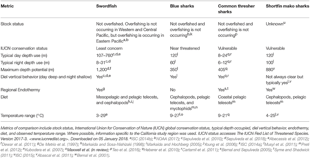
Table 1. Ecological comparison of swordfish, blue sharks, common thresher sharks, and shortfin mako sharks based on published sources.

Methods

Species and Environmental Data

Species occurrence data were obtained from the NOAA fisheries observer program from the California drift gillnet fishery, which operates at night along the US West Coast (Figure 1). This fishery targets swordfish, but also retains other species including common thresher sharks and shortfin mako sharks. Catch of all species, including bycaught species such as blue sharks, are recorded in the observer program which operates at ~15% coverage across the fishery. The catch data contained the presence or absence of an animal in each set, with species size data not universally available for analysis. The data were temporally limited to 1997 through 2017 to match the availability of environmental data, namely satellite-derived chlorophyll-a (Table 1). All analyses described below were performed using R statistical computing (R Core Team, 2017).

FIGURE 1

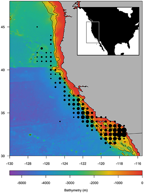
Figure 1. Study area off the US West Coast indicating the bathymetry (m; color scale) and location of fishing sets during 1997–2017 (dots) within the Regional Ocean Modeling System (ROMS) domain (inset). Fishing sets locations are aggregated to the nearest 0.5°, and dot size indicates relative frequency of sets. The 1,000 and 2,000 m bathymetric contours are shown.

A total of 16 environmental variables were available for inclusion in species distribution models, which included three static variables, 11 dynamic surface variables, and two dynamic subsurface variables (Table 2). Three static variables included bathymetry (z; ETOPO1 obtained from https://www.ngdc.noaa.gov/mgg/global/global.html, interpolated to 0.1°), rugosity (z_sd; calculated as the standard deviation of z over a 0.3° square), and lunar illumination from the “lunar” package in R. Lunar illumination was included in the static grouping as it does not require observation due to its definitive cyclical nature. Lunar illumination was chosen as the fishery gear is deployed at night and illumination is known to affect the vertical distribution of swordfish (Sepulveda et al., 2010; Lerner et al., 2012; Scales et al., 2017b). The majority of dynamic environmental data was sourced from daily fields of an ocean circulation model, namely a data assimilative configuration of the Regional Ocean Modeling System (ROMS) that covers the California Current System from 30 to 48 °N and from the coast to 134 °W at 0.1° (~10 km) horizontal resolution (http://oceanmodeling.ucsc.edu/ccsnrt version 2016a; Neveu et al., 2016). The ROMS 0.1° spatial resolution is considered sufficient for habitat modeling as this spatial scale combined with a fine temporal scale (daily) acts to minimize bias in similar species distribution models (Scales et al., 2017a). Vertical structure in the ROMS model is resolved by 42 terrain-following vertical levels (Veneziani et al., 2009). Importantly, the ROMS model employed here assimilates available data from satellites and in situ platforms (e.g., ships, moorings, buoys) to provide environmental information that is better than either the model or the observations in isolation. The temporal scale of our study spanned two ROMS iterations, a historical re-analysis (1980–2010; Neveu et al., 2016) and a near real-time product (2011-present) and as such all ROMS variables were assessed for consistency across the two temporal periods using a time-series analysis.

TABLE 2

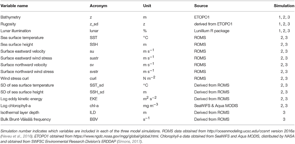
Table 2. Summary of 16 environmental variables included in species distribution models.

Eleven dynamic surface ROMS variables chosen included sea surface temperature (SST) and its standard deviation (SST_sd; calculated over a 0.3° square), sea surface height (SSH) and its standard deviation (SSH_sd; calculated over a 0.3° square), surface eastward and northward velocity (su; sv), surface eastward and northward wind stress (sustr; svstr), wind stress curl, and eddy kinetic energy (EKE) (Table 2). We also included chlorophyll-a as a dynamic surface variable, but as the assimilative ROMS model is purely physical, we used a combination of satellite-derived products (SeaWiFS and Aqua MODIS, distributed by NASA and obtained from SWFSC Environmental Research Division's ERDDAP; Simons, 2017). Chlorophyll-a and EKE were highly right skewed and were log_e transformed prior to analysis.

Dynamic subsurface ROMS variables included isothermal layer depth (ILD) and bulk buoyancy frequency (BBV, also known as Brunt-Väisälä frequency). Both variables provide indices of water column structure, respectively the depth of surface mixing and degree of stratification in the upper water column. ILD (m) was calculated as the depth corresponding to a 0.5°C temperature difference relative to sea surface temperature (Monterey and Levitus, 1997). Daily mean surface temperature was used as a reference point because the typical 10 m reference point is not suitable for regions with strong upwelling, like the California Current (de Boyer Montégut et al., 2004). ILD provides a daily horizontal field (0.1° resolution) comparable to dynamic surface variables (Scales et al., 2017b). BBV (s⁻¹) offers a measure of the upper water column stability and was averaged over the upper 200 m of the water column to produce a daily horizontal field (0.1° resolution), where higher BBV values indicate a more stable water column. In areas <200 m deep, BBV was averaged over the entire water column. The two-dimensional structure of ILD and BBV described water column properties best suited SDM development as the catch data used here were not vertically informed (i.e., depth of catch).

Species Distribution Models

Three species distribution models were built for each species (swordfish, blue sharks, common thresher sharks, and shortfin mako sharks) using fishery catch data. The probability of species presence was modeled as a function of environmental variables (described above) using a boosted regression tree (BRT) framework from the “dismo” R package (Elith et al., 2008). Three combinations of environmental variables were used to explore the importance of dynamic vertical variables on models. Simulation 1: static only variables (z, z_sd, lunar); simulation 2: static and dynamic surface variables with no vertical variables; simulation 3: models with static and dynamic surface variables and vertical variables (Table 2). Co-linearity between environmental variables was not a prohibitive issue as the BRT framework automatically handles any co-linearity effects (Elith et al., 2008). All BRT models were built using a Bernoulli family appropriate to the response variable of presence (1) and absence (0). The BRTs had a learning rate of 0.01, a tree complexity of 3, and a bag fraction of 0.6 (Elith et al., 2008). The resultant species distribution models describe the probability of species presence, here termed “habitat suitability” due to our use of fisheries catch data as a response variable.

Species distribution models were evaluated using explained deviance, Area Under the receiver operating Curve (AUC), and true skill statistic (TSS). Explained deviance (%) gives an indication of how well the model explains the data, while AUC and TSS assess the predictive performance of models on new data. Explained deviance was calculated as an average of 50 model iterations. This evaluation approach is possible because the bag fraction (0.6) of each model ensures a random selection of data to each tree, resulting in each model iteration being unique. The AUC and TSS were calculated as the average of 50 model iterations, where each iteration was built using 75% of the data and assessed against the remaining 25% of the data. This approach for model evaluation was done for each species (n = 4) and each model simulation (n = 3) and used a learning rate of 0.001 to improve convergence on the reduced dataset (75%). Differences in evaluation metrics between model simulations were assessed for significance using ANOVA and a Tukey Honest Significance Differences (HSD) post-hoc test (Fournier et al., 2017) in the R “stats” package (R Core Team, 2017).

Final SDMs were used to predict and visualize species habitat suitability on two example days, 1st December 2012 and 2015. December was chosen as fishery catch peaks during this month (Urbisci et al., 2016). 2012 represents a neutral year in the California Current ecosystem, with no strong ENSO influences (Bjorkstedt et al., 2012), while 2015 was a year when the California Current was strongly affected by the combination of an El Niño and pre-existing warm anomalies (Jacox et al., 2016). Habitat suitability predictions were made for each species (n = 4), and for model simulations 2 and 3 (dynamic simulations with and without vertical variables). The differences in habitat suitability between simulations 2 and 3 were calculated to visualize the effect of adding vertical variables into models.

Results

Species catch data along the California coast were not evenly distributed, with the majority of effort concentrated in the southern region (Figure 1). A total of 4,719 drift gillnet sets were used in the analysis. There were more swordfish present (n = 2986) than absent in these sets. In contrast, there were more shark species absent than present (blue sharks n = 2163; common thresher sharks n = 1074; shortfin mako sharks n = 2048) in sets.

Species distribution models revealed complex relationships among species presence and environmental variables. The relative importance of each variable varied among species, but the dynamic subsurface variables (BBV and ILD) ranked in the top six variables across all species (Figure 2; Table S1). The contribution of BBV and ILD was most prevalent in the swordfish model relative to the shark models (Figure 2).

FIGURE 2

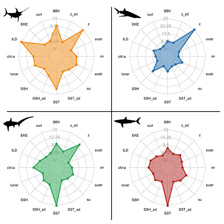
Figure 2. Spider plots of the relative influence (%) of each environmental variable within species distribution models: swordfish (yellow); blue sharks (blue); common thresher sharks (green); shortfin mako sharks (red). Variable acronyms are described in Table 2.

Variable response curves revealed how the probability of species presence was influenced by each variable (Figure 3; Figure S1). For brevity, we describe results for the two vertical variables (ILD, BBV; Figure 3), with the remaining variable response curves provided in the Supplementary Material (Figure S1). For swordfish, the probability of presence had a positive correlation with ILD (peaking 40–120 m) and a non-monotonic correlation with BBV (preference between 0.009 and 0.013 s⁻¹). For blue sharks, the probability of presence had a positive correlation with ILD (peaking 40–120 m) and a positive correlation with BBV (plateauing at 0.009 s⁻¹). For shortfin mako sharks, the probability of presence had a positive correlation with ILD (less steep slope between 20 and 120 m) and a negative correlation with BBV (plateauing at 0.009 s⁻¹). For common thresher sharks, the probability of presence had a positive correlation with ILD (sharp increase >70 m) and a complex non-linear correlation with BBV (two troughs at 0.009 and 0.013 s⁻¹).

FIGURE 3

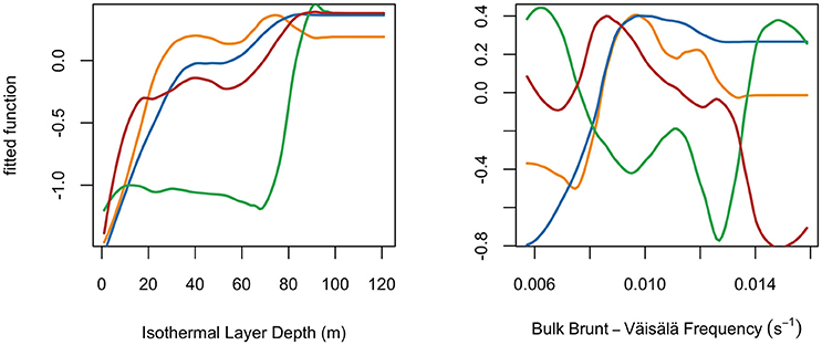
Figure 3. Species partial response curves for two example variables, Isothermal Layer Depth and Bulk Brunt-Väisälä frequency. Species indicated by color: swordfish (yellow), blue sharks (blue), common thresher sharks (green), and shortfin mako sharks (red). Lines use a loess smoother fitted to the boosted regression tree response curves.

The addition of dynamic surface and subsurface variables (simulations 2 and 3) to the static model (simulation 1) significantly improved model explanatory power and predictive performance across all species (Figure 4; Table 3; p < 0.001). Furthermore, the addition of vertical variables (simulation 3) to a non-vertical variable model (simulation 2) typically increased model explanatory power and predictive performance (Figure 4; Table 3). However, post-hoc analyses revealed the improvement in predictive performance between simulation 2 and 3 was not statistically significant for species with strong responses to bathymetry (blue sharks and common thresher sharks; Figure 4). Further, blue sharks were the only species where adding vertical variables (simulation 3) did not significantly improve explained deviance (Figure 4; Table 3). The addition of vertical variables (simulation 3) to a non-vertical variable model (simulation 2) also resulted in changes to dynamic variable response curves (Figure S2).

FIGURE 4

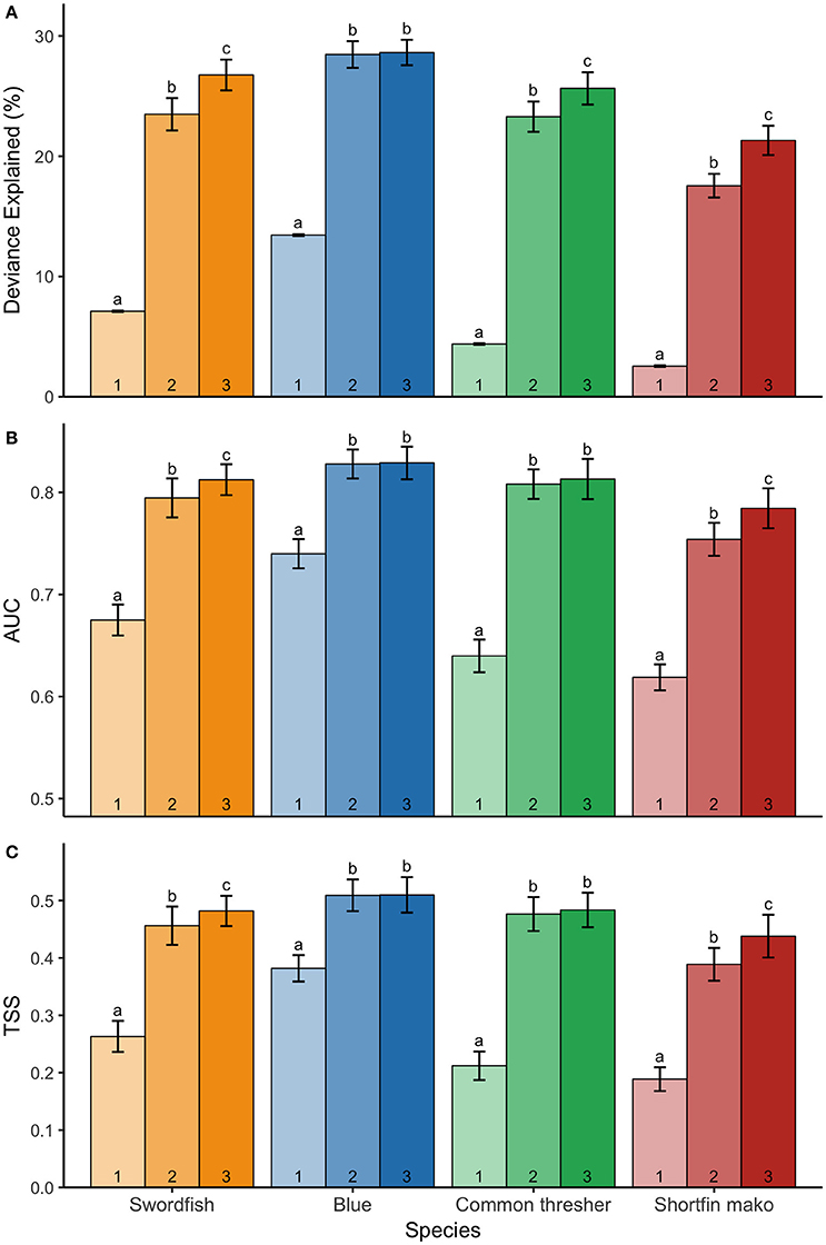
Figure 4. Mean ± S.D. (A) deviance explained; (B) AUC; and (C) TSS for three model simulations indicated numerically: simulation 1 (static variables only); simulation 2 (static and dynamic surface variables); and simulation 3 (static and dynamic surface and subsurface variables). Species' model simulations were run 50 times to generate mean ± S.D, with significance denoted by letters (ANOVA and Tukey HSD, p < 0.05). Models for each species are shown: swordfish (yellow), blue sharks (blue), common thresher sharks (green), and shortfin mako sharks (red). Letters are only comparable among simulations of the same species.

TABLE 3

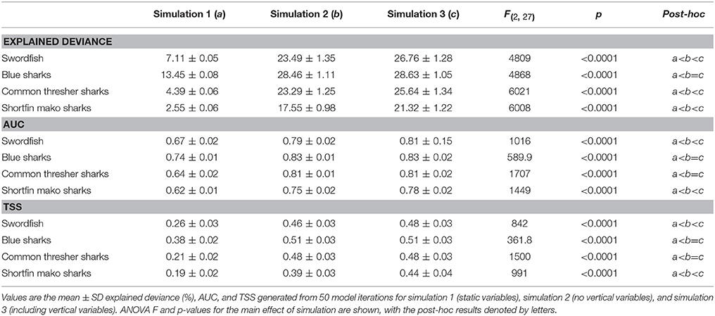
Table 3. ANOVA and Tukey HSD post-hoc results from species distribution model simulation comparison.

Predicted species' habitat suitability for 1st December 2012 and 2015 revealed spatial differences among species, with common thresher shark habitat predicted more suitable inshore of the 1,000 m isobath and the other three species habitat predicted to be more suitable offshore of the 1,000 m isobath and in the Southern California Bight (Figure 5; Figure S3). The effect of adding of ILD and BBV to species distribution models was evident in each species spatial prediction (Figure 5; Figure S3). Differences in the predicted habitat suitability between simulations 2 and 3 indicated that the vertical variables ILD and BBV contributed to model predictions primarily at a sub-mesoscale level (<100 km). Comparison of species spatial predictions between a neutral year (2012; Figure 5) and an El Niño year (2015; Figure S3) revealed that during 2015 all species predicted habitat expanded, and the contribution of ILD and BBV was more prominent in the swordfish and blue shark models.

FIGURE 5

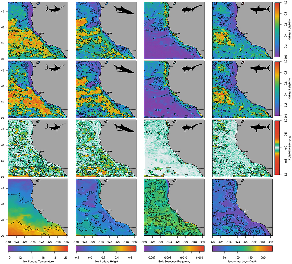
Figure 5. Predicted habitat suitability for each species for an example day, 1 December 2012. The first row shows predicted habitats using simulation 2 (static and dynamic surface variables), the second row shows predicted habitats using simulation 3 (static and dynamic surface and subsurface variables), and the third row shows the difference in probabilities between simulations 2 and 3. The fourth row shows four example dynamic variables for the same day (Sea Surface Temperature, Sea Surface Height, Bulk Buoyancy Frequency, and Isothermal Layer Depth). Species are indicated by a black silhouette: swordfish (first column), blue sharks (second column), common thresher sharks (third column), and shortfin mako sharks (fourth column). Contours on the first and second row are at 0.6 and 0.2, contours on the third row are at 0.1 and −0.1, and contours on the fourth row equate to the 25 and 75% quantiles.

Discussion

Species distribution models (SDMs) are increasingly used to characterize and understand the distributions of marine species. The prevalence of vertical movement behavior in pelagic top predators substantiates the importance of integrating vertical water column structure into SDMs. Using evaluation metrics for SDMs, we showed that integrating dynamic subsurface variables increased explanatory power across all species models, although the degree of improvement to model predictive performance was species-dependent. Inter-specific variability in results is likely a result of individual species ecology, where species with strong correlations with static variables were less affected by the addition of dynamic subsurface variables (e.g., blue sharks). The positive effect of including dynamic subsurface variables supports their utility in marine SDM development and encourages further exploration of the vertical dimension to species' horizontal distributions and movements. The use of dynamic subsurface variables in SDM development provided further understanding of the processes driving species distributions, which has clear implications for the ongoing management and conservation of marine megafauna.

Species Ecological Responses to Variables

The SDMs built here reveal the complex responses four top predators have to static and dynamic environmental variables. The wide range of variables used in model development represent direct (e.g., temperature-dependent physiological effects; Altringham and Block, 1997; Brown, 2004) and indirect (e.g., chlorophyll-a as an indicator of productivity; Armstrong et al., 1995; Polovina et al., 2008) effects on the distribution of these top predators. Here, the dynamic subsurface variables included in SDMs, namely bulk buoyancy frequency (BBV) and isothermal layer depth (ILD), likely have direct and indirect effects on top predator distribution and therefore influence their susceptibility to catch (see below). These variables characterized subsurface water properties on a horizontal plane, and in doing so indicated relative temperature (direct effects) and availability of prey fields (indirect effects).

Bulk buoyancy frequency (BBV) quantifies water column stability, where high BBV values reflect a more stable water column. Increased stability (a more stratified water column) acts as a barrier for upward nutrient flux into the photic zone, affecting the productivity and distribution of prey fields (Haug et al., 1986; Susini-Ribeiro et al., 2013; Behrenfeld and Boss, 2014). Here, top predator response to BBV differs among species, with swordfish, blue sharks, and shortfin mako sharks showing an increased probability of occurrence in areas with intermediate BBV values. Lower BBV values correspond to waters that are highly mixed and less stable, typical of upwelled waters that are cold and oxygen poor (Grantham et al., 2004). While these species are physiologically and biomechanically equipped for foraging in cold and hypoxic waters (Table 1; Dickson and Graham, 2004; Wegner et al., 2010; Abecassis et al., 2012), surface waters support recovery from deep vertical dives by allowing thermal regulation of body temperature and a reduction of oxygen debt (Dagorn et al., 2000; Dewar et al., 2011). As a result, intermediate BBV levels may provide a middle ground between prey availability (low BBV values) and suitability of surface waters for recovering from vertical movements (high BBV values). In contrast, common thresher sharks preferred extreme BBV values (low and high), which likely reflects their predominantly coastal distribution (shallow bathymetry preference) as such areas can have the most extreme BBV values (Figure 5).

Isothermal layer depth (ILD) was an important variable in the SDMs, and its relative influence was similar among species. Isothermal layer depth is a proxy for mixed layer depth, and indicates the depth where physical water properties (i.e., temperature, salinity, nutrients, oxygen) change dramatically (Robison, 2004). All four species showed a preference for waters with deeper ILDs which indicates a thick homogenous surface layer in the epipelagic zone where temperature and oxygen are higher. This surface layer may provide a thermal and oxygen refuge for pelagic predators (Prince and Goodyear, 2006; Dewar et al., 2011; Carlisle et al., 2017), as many pelagic predators, including the study species, spend much of their time in surface waters despite foraging in waters below the mixed layer (Table 1). The common thresher shark partial response curve showed a unique response to ILD, which appears to be related to a weak negative correlation between ILD and SST (−0.54 Pearson correlation coefficient). As SST has a greater relative influence on common thresher sharks than ILD, the preference for colder SST values better describes occurrence, which results in no strong pattern seen with ILD <70m. This disconnect between partial effect curves is typical, and while plot interpretation can be challenging when variables are correlated, these plots represent an effective way of visualizing the effects of each variable (Elith et al., 2008). Given the response common thresher sharks showed here, future work could explore the utility of other subsurface variables in describing their habitat suitability, including model-based upwelling indices (e.g., Jacox et al., 2014) that would spatially align with their predominantly coastal distribution.

Integration of the Vertical Dimension in SDMs

Integrating dynamic subsurface variables into marine SDMs had a positive effect on describing the horizontal habitat suitability of four pelagic species. The mechanism behind this result is likely a combination of the main effect of ILD and BBV within the model framework, as well as the co-variation with other variables (Figure S2). This co-variation occurs as a result of including multiple variables in the statistical framework. While certain variables had a higher relative effect than others, no single variable could perform as well as the multi-variable models, or even perform at a standard required for conservation planning (AUC > 0.75; Table S2) (Pearce and Ferrier, 2000). There is a trade-off in the number of variables to include in a SDM, where a simple model is easier to interpret but may come at a cost of decreased predictive performance, while a complex model is challenging to interpret ecologically (and especially as response curves change) but may have increased predictive performance (Friedman et al., 2001). Furthermore, there is potential for overfitting to occur as the number of variables included in SDMs increases, however regularization methods advised for boosted regression trees reduces the risk of overfitting (Elith et al., 2008). Future research could build on our results by including additional species and additional model frameworks (e.g., generalized linear and additive models; machine learning). There is further scope to explore subsurface variables in SDMs (e.g., oxygen) and we acknowledge that the subsurface variables explored here (BBV and ILD) may not be sufficient for all marine species. Typically, environmental variables included in SDMs are best informed from a priori expectations based on species ecology (Fourcade et al., 2018).

Using ocean circulation models for SDM development can maximize the use of catch data and allow model prediction to be done on large spatiotemporal scales. However, not all ocean circulation models are equal and care must be taken to ensure outputs are appropriate for use. The dynamic surface variables obtained from this ocean circulation model are a best-case scenario of data availability, in that data from satellites and quarterly in situ data surveys are incorporated (data assimilative) but typical issues with satellite-derived information are avoided (i.e., cloud cover, patchiness, resolution mismatch, temporal span of products; Scales et al., 2017a). Ocean circulation models also provide a consistent framework to access data across periods of changing observational assets (i.e., different satellite eras). Output from regional ocean models, and especially data-assimilative models, is unfortunately limited to certain regions and time periods such that its use will be precluded in some SDM development. However, when data are available for the time period and spatial domain of interest, the added benefits of using ocean circulation data can be powerful (Becker et al., 2016; Scales et al., 2017b).

Integrating dynamic subsurface variables improved the explanatory power and predictive performance of SDMs for highly migratory species. The benefits to model explanatory power support the future use and inclusion of such variables, where possible, to get the best ecological understanding of the environmental drivers on species distributions. Improvements to predictive performance, while significant, were not large for a model that already incorporates many dynamic surface variables. For an operational version of such a model (e.g., Hazen et al., 2018) the benefits of including subsurface variables should be weighed against the resources needed to obtain them and evaluate their contribution. However, more generally there is added benefit in using ocean circulation models—whether variables are vertical or horizontal, or both—in SDM applications, as ocean circulation models: (i) eliminate data gaps that are prevalent in satellite data and in situ sources; (ii) provide continuity across periods of changing observational assets; (iii) provide all variables at common spatial and temporal resolutions; and (iv) can be configured to predict into the future. Operational models require continuous collection and collation of data products, a process that is greatly streamlined by having a single source for ocean circulation model output rather than multiple remotely sensed data providers. This improved efficacy can support conservation planning, decision-making, and management (Hobday et al., 2018; Stelzenmüller et al., 2018) on near real-time (Maxwell et al., 2015), seasonal (Brodie et al., 2017), and longer timescales (Almpanidou et al., 2016; Ban et al., 2016).

Author Contributions

SB, MJ, SJB, HW, HD, KS, SM, DB, CE, LC, RL, and EH contributed to writing and reviewing of the manuscript. SB, MJ, SJB, HW, KS, and EH contributed to project design. SB, MJ, CE, HD, KS, DB, and SM contributed to data collation. SB conducted analyses and prepared manuscript figures.

Conflict of Interest Statement

The authors declare that the research was conducted in the absence of any commercial or financial relationships that could be construed as a potential conflict of interest.

Acknowledgments

Funding was provided by NASA Earth Science Division/Applied Sciences ROSES Program (NNH12ZDA001N-ECOF); NOAA Modeling, Analysis, Predictions and Projections MAPP Program (NA17OAR4310108); NOAA Coastal and Ocean Climate Application COCA Program (NA17OAR4310268); NOAA's Integrated Ecosystem Assessment program; NOAA Bycatch Reduction Engineering Program Funding Opportunity (NA14NMF4720312); NOAA NMFS Office of Science and Technology; and the California Sea Grant Program (NA140AR4170075). We also thank Lucie Hazen for project management, and Suzy Kohin for assistance and advice on data compilation.

Supplementary Material

The Supplementary Material for this article can be found online at: https://www.frontiersin.org/articles/10.3389/fmars.2018.00219/full#supplementary-material

References

Abascal, F. J., Quintans, M., Ramos-Cartelle, A., and Mejuto, J. (2011). Movements and environmental preferences of the shortfin mako, Isurus oxyrinchus, in the southeastern Pacific Ocean. Mar. Biol. 158, 1175–1184. doi: 10.1007/s00227-011-1639-1

CrossRef Full Text | Google Scholar

Abecassis, M., Dewar, H., Hawn, D., and Polovina, J. (2012). Modeling swordfish daytime vertical habitat in the North Pacific Ocean from pop-up archival tags. Mar. Ecol. Prog. Ser. 452, 219–236. doi: 10.3354/meps09583

CrossRef Full Text | Google Scholar

Almpanidou, V., Schofield, G., Kallimanis, A. S., Türkozan, O., Hays, G. C., and Mazaris, A. D. (2016). Using climatic suitability thresholds to identify past, present and future population viability. Ecol. Indic. 71, 551–556. doi: 10.1016/j.ecolind.2016.07.038

CrossRef Full Text | Google Scholar

Altringham, J. D., and Block, B. A. (1997). Why do tuna maintain elevated slow muscle temperatures? Power output of muscle isolated from endothermic and ectothermic fish. J. Exp. Biol. 200, 2617–2627.

PubMed Abstract | Google Scholar

Armstrong, R. A., Sarmiento, J. L., and Slater, R. D. (1995). “Monitoring ocean productivity by assimilating satellite chlorophyll into ecosystem models,” in Ecological Time Series, eds T. M. Powell and J. H. Steele (Boston, MA: Springer), 371–390.

Google Scholar

Ban, S. S., Alidina, H. M., Okey, T. A., Gregg, R. M., and Ban, N. C. (2016). Identifying potential marine climate change refugia: a case study in Canada's Pacific marine ecosystems. Glob. Ecol. Conserv. 8, 41–54. doi: 10.1016/j.gecco.2016.07.004

CrossRef Full Text | Google Scholar

Becker, E. A., Forney, K. A., Fiedler, P. C., Barlow, J., Chivers, S. J., Edwards, C. A., et al. (2016). Moving towards dynamic ocean management: how well do modeled ocean products predict species distributions? Remote Sens. 8:149. doi: 10.3390/rs8020149

CrossRef Full Text | Google Scholar

Behrenfeld, M. J., and Boss, E. S. (2014). Resurrecting the ecological underpinnings of ocean plankton blooms. Ann. Rev. Mar. Sci. 6, 167–194. doi: 10.1146/annurev-marine-052913-021325

PubMed Abstract | CrossRef Full Text | Google Scholar

Bernal, D., and Sepulveda, C. A. (2005). Evidence for temperature elevation in the aerobic swimming musculature of the common thresher shark, Alopias vulpinus. Copeia 2005, 146–151. doi: 10.1643/CP-04-180R1

CrossRef Full Text | Google Scholar

Bernal, D., Sepulveda, C., and Graham, J. B. (2001). Water-tunnel studies of heat balance in swimming mako sharks. J. Exp. Biol. 204, 4043–4054.

PubMed Abstract | Google Scholar

Bestley, S., Jonsen, I. D., Hindell, M. A., Harcourt, R. G., and Gales, N. J. (2015). Taking animal tracking to new depths: synthesizing horizontal–vertical movement relationships for four marine predators. Ecology 96, 417–427. doi: 10.1890/14-0469.1

PubMed Abstract | CrossRef Full Text | Google Scholar

Bjorkstedt, E. P., Goericke, R., McClatchie, S., Weber, E., Watson, W., Lo, N., et al. (2012). State of the California current 2011–2012: ecosystems respond to local forcing as La Niña wavers and wanes. CalCOFI Report, 53.

Block, B., Jonsen, I., Jorgensen, S., Winship, A., Shaffer, S. A., Bograd, S., et al. (2011). Tracking apex marine predator movements in a dynamic ocean. Nature 475, 86–90. doi: 10.1038/nature10082

PubMed Abstract | CrossRef Full Text | Google Scholar

Brodie, S., Hobday, A. J., Smith, J. A., Everett, J. D., Taylor, M. D., Gray, C. A., et al. (2015). Modelling the oceanic habitats of two pelagic species using recreational fisheries data. Fish. Oceanogr. 24, 463–477. doi: 10.1111/fog.12122

CrossRef Full Text | Google Scholar

Brodie, S., Hobday, A. J., Smith, J. A., Spillman, C. M., Hartog, J. R., Everett, J. D., et al. (2017). Seasonal forecasting of dolphinfish distribution in eastern Australia to aid recreational fishers and managers. Deep Sea Res. Part II Top. Stud. Oceanogr. 140, 222–229. doi: 10.1016/j.dsr2.2017.03.004

CrossRef Full Text | Google Scholar

Brown, J. H. (2004). Toward a metabolic theory of ecology. Ecology 85, 1771–1789. doi: 10.1890/03-9000

CrossRef Full Text | Google Scholar

Carlisle, A. B., Kochevar, R. E., Arostegui, M. C., Ganong, J. E., Castleton, M., Schratwieser, J., et al. (2017). Influence of temperature and oxygen on the distribution of blue marlin (Makaira nigricans) in the Central Pacific. Fish. Oceanogr. 26, 34–48. doi: 10.1111/fog.12183

CrossRef Full Text | Google Scholar

Cartamil, D. P., Sepulveda, C. A., Wegner, N. C., Aalbers, S. A., Baquero, A., and Graham, J. B. (2011). Archival tagging of subadult and adult common thresher sharks (Alopias vulpinus) off the coast of southern California. Mar. Biol. 158, 935–944. doi: 10.1007/s00227-010-1620-4

PubMed Abstract | CrossRef Full Text | Google Scholar

Dagorn, L., Bach, P., and Josse, E. (2000). Movement patterns of large bigeye tuna (Thunnus obesus) in the open ocean, determined using ultrasonic telemetry. Mar. Biol. 136, 361–371. doi: 10.1007/s002270050694

CrossRef Full Text | Google Scholar

de Boyer Montégut, C., Madec, G., Fischer, A. S., Lazar, A., and Iudicone, D. (2004). Mixed layer depth over the global ocean: an examination of profile data and a profile-based climatology. J. Geophys. Res. Oceans 109:C12003. doi: 10.1029/2004JC002378

CrossRef Full Text | Google Scholar

Dell, J., Wilcox, C., and Hobday, A. J. (2011). Estimation of yellowfin tuna (Thunnus albacares) habitat in waters adjacent to Australia's East Coast: making the most of commercial catch data. Fish. Oceanogr. 20, 383–396. doi: 10.1111/j.1365-2419.2011.00591.x

CrossRef Full Text | Google Scholar

De Metrio, G., Ditrich, H., and Palmieri, G. (1997). Heat-producing organ of the swordfish (Xiphias gladius): a modified eye muscle. J. Morphol. 234, 89–96.

PubMed Abstract | Google Scholar

Dewar, H., Prince, E. D., Musyl, M. K., Brill, R. W., Sepulveda, C., Luo, J., et al. (2011). Movements and behaviors of swordfish in the Atlantic and Pacific Oceans examined using pop-up satellite archival tags. Fish. Oceanogr. 20, 219–241. doi: 10.1111/j.1365-2419.2011.00581.x

CrossRef Full Text | Google Scholar

Dickson, K. A., and Graham, J. B. (2004). Evolution and consequences of endothermy in fishes. Physiol. Biochem. Zool. 77, 998–1018. doi: 10.1086/423743

PubMed Abstract | CrossRef Full Text | Google Scholar

Elith, J., Graham, C. H., Anderson, R. P., Dudik, M., Ferrier, S., Guisan, A., et al. (2006). Novel methods improve prediction of species' distributions from occurrence data. Ecography 29, 129–151. doi: 10.1111/j.2006.0906-7590.04596.x

CrossRef Full Text | Google Scholar

Elith, J., and Leathwick, J. R. (2009). Species distribution models: ecological explanation and prediction across space and time. Annu. Rev. Ecol. Evol. Syst. 40, 677–697. doi: 10.1146/annurev.ecolsys.110308.120159

CrossRef Full Text | Google Scholar

Elith, J., Leathwick, J. R., and Hastie, T. (2008). A working guide to boosted regression trees. J. Anim. Ecol. 77, 802–813. doi: 10.1111/j.1365-2656.2008.01390.x

PubMed Abstract | CrossRef Full Text | Google Scholar

Fourcade, Y., Besnard, A. G., and Secondi, J. (2018). Paintings predict the distribution of species, or the challenge of selecting environmental predictors and evaluation statistics. Glob. Ecol. Biogeogr. 27, 245–256. doi: 10.1111/geb.12684

CrossRef Full Text | Google Scholar

Fournier, A., Barbet-Massin, M., Rome, Q., and Courchamp, F. (2017). Predicting species distribution combining multi-scale drivers. Glob. Ecol. Conserv. 12, 215–226. doi: 10.1016/j.gecco.2017.11.002

CrossRef Full Text | Google Scholar

Friedman, J., Hastie, T., and Tibshirani, R. (2001). The Elements of Statistical Learning. New York, NY: Springer.

Google Scholar

Grantham, B. A., Chan, F., Nielsen, K. J., Fox, D. S., Barth, J. A., Huyer, A., et al. (2004). Upwelling-driven nearshore hypoxia signals ecosystem and oceanographic changes in the northeast Pacific. Nature 429, 749–754. doi: 10.1038/nature02605

PubMed Abstract | CrossRef Full Text | Google Scholar

Guisan, A., and Thuiller, W. (2005). Predicting species distribution: offering more than simple habitat models. Ecol. Lett. 8, 993–1009. doi: 10.1111/j.1461-0248.2005.00792.x

CrossRef Full Text | Google Scholar

Haug, T., Kjørsvik, E., and Solemdal, P. (1986). Influence of some physical and biological factors on the density and vertical distribution of Atlantic halibut Hippoglossus hippoglossus eggs. Mar. Ecol. Prog. Ser. 33, 207–216. doi: 10.3354/meps033207

CrossRef Full Text | Google Scholar

Hazen, E., Scales, K., Maxwell, S., Briscoe, D., Welch, H., Bograd, S., et al. (2018). A dynamic ocean management tool to reduce bycatch and support sustainable fisheries. Sci. Adv. 4:eaar3001. doi: 10.1126/sciadv.aar3001

PubMed Abstract | CrossRef Full Text | Google Scholar

Heberer, C., Aalbers, S., Bernal, D., Kohin, S., DiFiore, B., and Sepulveda, C. (2010). Insights into catch-and-release survivorship and stress-induced blood biochemistry of common thresher sharks (Alopias vulpinus) captured in the southern California recreational fishery. Fish. Res. 106, 495–500. doi: 10.1016/j.fishres.2010.09.024

CrossRef Full Text | Google Scholar

Hobday, A. J., Spillman, C. M., Eveson, J. P., Hartog, J. R., Zhang, X., and Brodie, S. (2018). A framework for combining seasonal forecasts and climate projections to aid risk management for fisheries and aquaculture. Front. Mar. Sci. 5:137. doi: 10.3389/fmars.2018.00137

CrossRef Full Text | Google Scholar

Huisman, J., Thi, N. N. P., Karl, D. M., and Sommeijer, B. (2006). Reduced mixing generates oscillations and chaos in the oceanic deep chlorophyll maximum. Nature 439, 322–325. doi: 10.1038/nature04245

PubMed Abstract | CrossRef Full Text | Google Scholar

ISC (2014a). Annex 13 Stock Assessment and Future Projections of Blue Shark in the North Pacific Ocean. Report of the Shark Working Group. International Scientific Committee for Tuna and Tuna-like Species in the North Pacific Ocean.

ISC (2014b). North Pacific Swordfish (Xiphiaus gladius) Stock Assessment in 2014. Report of the Billfish Working Group. International Scientific Committee for Tuna and Tuna-like Species in the North Pacific Ocean.

ISC (2015). Annex 12 Indicator-based Analysis of the Status of Shortfin Mako Shark in the North Pacific Ocean. Report of the shark working group. International Scientific Committee for Tuna and Tuna-like Species in the North Pacific Ocean.

Jacox, M. G., Hazen, E. L., Zaba, K. D., Rudnick, D. L., Edwards, C. A., Moore, A. M., et al. (2016). Impacts of the 2015–2016 El Niño on the california current system: early assessment and comparison to past events. Geophys. Res. Lett. 43, 7072–7080. doi: 10.1002/2016GL069716

CrossRef Full Text | Google Scholar

Jacox, M. G., Moore, A. M., Edwards, C. A., and Fiechter, J. (2014). Spatially resolved upwelling in the california current System and its connections to climate variability. Geophys. Res. Lett. 41, 3189–3196. doi: 10.1002/2014GL059589

CrossRef Full Text | Google Scholar

Kara, A. B., Rochford, P. A., and Hurlburt, H. E. (2003). Mixed layer depth variability over the global ocean. J. Geophys. Res. Oceans 108:3079. doi: 10.1029/2000JC000736

CrossRef Full Text | Google Scholar

Kubodera, T., Watanabe, H., and Ichii, T. (2007). Feeding habits of the blue shark, Prionace glauca, and salmon shark, Lamna ditropis, in the transition region of the Western North Pacific. Rev. Fish Biol. Fish. 17:111. doi: 10.1007/s11160-006-9020-z

CrossRef Full Text | Google Scholar

Lerner, J. D, Kerstetter, D. W, Prince, E. D., Talaue-McManus, L., Orbesen, E. S., Mariano, A., et al. (2012). Swordfish vertical distribution and habitat use in relation to diel and lunar cycles in the western north atlantic. Trans. Am. Fish. Soc. 142, 95–104. doi: 10.1080/00028487.2012.720629

CrossRef Full Text | Google Scholar

Mannocci, L., Boustany, A. M., Roberts, J. J., Palacios, D. M., Dunn, D. C., Halpin, P. N., et al. (2017). Temporal resolutions in species distribution models of highly mobile marine animals: recommendations for ecologists and managers. Divers. Distrib. 23, 1098–1109. doi: 10.1111/ddi.12609

CrossRef Full Text | Google Scholar

Markaida, U., and Hochberg, F. (2005). Cephalopods in the diet of swordfish (Xiphias gladius) caught off the west coast of Baja California, Mexico. Pac. Sci. 59, 25–41. doi: 10.1353/psc.2005.0011

CrossRef Full Text | Google Scholar

Markaida, U., and Sosa-Nishizaki, O. (1998). Food and Feeding Habits of Swordfish, Xiphias Gladius L., off Western Baja California. Biology and Fisheries of Swordfish, Xiphias Gladius. NOAA Technical Report.

Maxwell, S. M., Hazen, E. L., Lewison, R. L., Dunn, D. C., Bailey, H., Bograd, S. J., et al. (2015). Dynamic ocean management: defining and conceptualizing real-time management of the ocean. Mar. Policy 58, 42–50. doi: 10.1016/j.marpol.2015.03.014

CrossRef Full Text | Google Scholar

Monterey, G. I., and Levitus, S. (1997). Seasonal Variability of Mixed Layer Depth for the World Ocean. Washington, DC: US Department of Commerce, National Oceanic and Atmospheric Administration, National Environmental Satellite, Data, and Information Service.

Musyl, M. K., Brill, R. W., Curran, D. S., Fragoso, N. M., McNaughton, L. M., Nielsen, A., et al. (2011). Postrelease survival, vertical and horizontal movements, and thermal habitats of five species of pelagic sharks in the central Pacific Ocean. Fish. Bull. 109, 341–368.

Google Scholar

Neveu, E., Moore, A. M., Edwards, C. A., Fiechter, J., Drake, P., Crawford, W. J., et al. (2016). An historical analysis of the California Current circulation using ROMS 4D-Var: system configuration and diagnostics. Ocean Modell. 99, 133–151. doi: 10.1016/j.ocemod.2015.11.012

CrossRef Full Text | Google Scholar

NOAA (2017). National Marine and Fisheries Service 3rd Quarter 2017 Update. Table, A. Summary of Stock Status for FSSI Stocks. National Oceanic and Atmospheric Administration.

Pearce, J., and Ferrier, S. (2000). Evaluating the predictive performance of habitat models developed using logistic regression. Ecol. Modell. 133, 225–245. doi: 10.1016/S0304-3800(00)00322-7

CrossRef Full Text | Google Scholar

Polovina, J. J., Howell, E. A., and Abecassis, M. (2008). Ocean's least productive waters are expanding. Geophys. Res. Lett. 35:L03618. doi: 10.1029/2007GL031745

CrossRef Full Text | Google Scholar

Preti, A., Soykan, C. U., Dewar, H., Wells, R. D., Spear, N., and Kohin, S. (2012). Comparative feeding ecology of shortfin mako, blue and thresher sharks in the California Current. Environ. Biol. Fishes 95, 127–146. doi: 10.1007/s10641-012-9980-x

CrossRef Full Text | Google Scholar

Prince, E. D., and Goodyear, C. P. (2006). Hypoxia-based habitat compression of tropical pelagic fishes. Fish. Oceanogr. 15, 451–464. doi: 10.1111/j.1365-2419.2005.00393.x

CrossRef Full Text | Google Scholar

R Core Team (2017). R: A Language and Environment for Statistical Computing. R Foundation for Statistical Computing. Vienne: R Core Team.

Robinson, L. M., Elith, J., Hobday, A. J., Pearson, R. G., Kendall, B. E., Possingham, H. P., et al. (2011). Pushing the limits in marine species distribution modelling: lessons from the land present challenges and opportunities. Glob. Ecol. Biogeogr. 20, 789–802. doi: 10.1111/j.1466-8238.2010.00636.x

CrossRef Full Text | Google Scholar

Robinson, N. M., Nelson, W. A., Costello, M. J., Sutherland, J. E., and Lundquist, C. J. (2017). A systematic review of marine-based Species Distribution Models (SDMs) with recommendations for best practice. Front. Mar. Sci. 4:421. doi: 10.3389/fmars.2017.00421

CrossRef Full Text | Google Scholar

Robison, B. H. (2004). Deep pelagic biology. J. Exp. Mar. Biol. Ecol. 300, 253–272. doi: 10.1016/j.jembe.2004.01.012

CrossRef Full Text | Google Scholar

Scales, K. L., Hazen, E. L., Jacox, M. G., Edwards, C. A., Boustany, A. M., Oliver, M. J., et al. (2017a). Scale of inference: on the sensitivity of habitat models for wide-ranging marine predators to the resolution of environmental data. Ecography 40, 210–220. doi: 10.1111/ecog.02272

CrossRef Full Text | Google Scholar

Scales, K. L., Hazen, E. L., Maxwell, S. M., Dewar, H., Kohin, S., Jacox, M. G., et al. (2017b). Fit to predict? Eco-informatics for predicting the catchability of a pelagic fish in near real time. Ecol. Appl. 27, 2313–2329. doi: 10.1002/eap.1610

PubMed Abstract | CrossRef Full Text | Google Scholar

Schroeder, I. D., Santora, J. A., Moore, A. M., Edwards, C. A., Fiechter, J., Hazen, E. L., et al. (2014). Application of a data-assimilative regional ocean modeling system for assessing California Current System ocean conditions, krill, and juvenile rockfish interannual variability. Geophys. Res. Lett. 41, 5942–5950. doi: 10.1002/2014GL061045

CrossRef Full Text | Google Scholar

Sepulveda, C. A., Knight, A., Nasby-Lucas, N., and Domeier, M. L. (2010). Fine-scale movements of the swordfish Xiphias gladius in the Southern California Bight. Fish. Oceanogr. 19, 279–289. doi: 10.1111/j.1365-2419.2010.00543.x

CrossRef Full Text | Google Scholar

Sepulveda, C. A., Aalbers Scott, A., Heberer, C., Kohin, S., and Dewar, H. (2018). Movements and behaviors of swordfish Xiphias gladius in the United States Pacific Leatherback Conservation Area. Fish. Oceanogr. 27, 381–394. doi: 10.1111/fog.12261

CrossRef Full Text | Google Scholar

Simons, R. A. (2017). ERDDAP. Monterey, CA: NOAA/NMFS/SWFSC/ERD. Available online at: https://coastwatch.pfeg.noaa.gov/erddap

Stelzenmüller, V., Coll, M., Mazaris, A. D., Giakoumi, S., Katsanevakis, S., Portman, M. E., et al. (2018). A risk-based approach to cumulative effect assessments for marine management. Sci. Total Environ. 612, 1132–1140. doi: 10.1016/j.scitotenv.2017.08.289

PubMed Abstract | CrossRef Full Text | Google Scholar

Susini-Ribeiro, S. M., Pompeu, M., Gaeta, S. A., de Souza, J. S., and Masuda, L. S. (2013). Topographical and hydrographical impacts on the structure of microphytoplankton assemblages on the Abrolhos Bank region, Brazil. Cont. Shelf Res. 70, 88–96. doi: 10.1016/j.csr.2013.09.023

CrossRef Full Text | Google Scholar

Syme, D. A., and Shadwick, R. E. (2011). Red muscle function in stiff-bodied swimmers: there and almost back again. Philos. Trans. R. Soc. B Biol. Sci. 366, 1507–1515. doi: 10.1098/rstb.2010.0322

PubMed Abstract | CrossRef Full Text | Google Scholar

Teo, S., Rodrigues, E., and Sosa-Nishizaki, O. (2016). “Status of common thresher sharks, Alopias Vulpinus, along the west coast of North America,” in Technical Memorandum. San Diego, CA: National Marine and Fisheries Service, National Oceanic and Atmospheric Administration.

Google Scholar

Urbisci, L. C., Stohs, S. M., and Piner, K. R. (2016). From sunrise to sunset in the California drift gillnet fishery: an examination of the effects of time and area closures on the catch and catch rates of pelagic species. Mar. Fish. Rev. 78, 3–4. doi: 10.7755/MFR.78.3–4.1

CrossRef Full Text | Google Scholar

Veneziani, M., Edwards, C., Doyle, J., and Foley, D. (2009). A central California coastal ocean modeling study: 1. Forward model and the influence of realistic versus climatological forcing. J. Geophys. Res. Oceans 114:C04015. doi: 10.1029/2008JC004774

CrossRef Full Text | Google Scholar

Wegner, N. C., Sepulveda, C. A., Bull, K. B., and Graham, J. B. (2010). Gill morphometrics in relation to gas transfer and ram ventilation in high-energy demand teleosts: scombrids and billfishes. J. Morphol. 271, 36–49. doi: 10.1002/jmor.10777

PubMed Abstract | CrossRef Full Text | Google Scholar

Young, J., Lansdell, M., Riddoch, S., and Revill, A. (2006). Feeding ecology of broadbill swordfish, Xiphias gladius, off eastern Australia in relation to physical and environmental variables. Bull. Mar. Sci. 79, 793–809.

Google Scholar