Assessing the Use of Area- and Time-Averaging Based on Known De-correlation Scales to Provide Satellite Derived Sea Surface Temperatures in Coastal Areas

Introduction

Water temperature is an important predictor of coastal diversity (Tittensor et al., 2010) and distribution (Block et al., 2011; Last et al., 2011; Wernberg et al., 2011) across a wide range of taxa. This is not surprising given that temperature is a key factor influencing reproduction (Pankhurst, 1997; Byrne et al., 2009), survival (Pepin, 1991; Eggert, 2012), growth (Morrongiello and Thresher, 2015; Singh and Singh, 2015) and behavior (Biro et al., 2010; Allan et al., 2015) of many marine species. Satellite derived sea surface temperature (SST) measurements are widely used as a proxy for water temperature (Block et al., 2011; Brodie et al., 2015), due to readily available data, broad spatial coverage and long-time series (albeit at low spatial resolution) in the absence of in situ recordings (which are often at short time scales and spatially limited). Although such (skin) SST measurements are only representative of the first microns of the sea surface (or ~10 m depth if foundation SST is used), they are regularly used as a proxy for temperatures at greater water depths (≥10 m) in ecological and biological studies (e.g., animal tracking: Papastamatiou et al., 2013; Lea et al., 2015; fisheries data- Brodie et al., 2015; Montero-Serra et al., 2015). SST, however, may not be available for coastal areas due to contamination in the satellite-derived images [noisier radar returns from land and sea (Brooks et al., 1990) and improper instrument corrections (Shum et al., 1998)]. In addition, previous studies have demonstrated biases in SST data when comparing it to in situ measurements within coastal areas (Smale and Wernberg, 2009; Lathlean et al., 2011; Stobart et al., 2016), with some studies recording up to 6°C differences (Smit et al., 2013). These biases are due to contamination of the satellite processing due to the presence of coastal features such as the shoreline, estuaries and embayments as well as complex coastal dynamics such as tides and upwelling (Smit et al., 2013) that vary over short spatial scales. Despite this well documented bias of satellite SST data in coastal areas, no studies have assessed if using spatial area averaging (based on known decorrelation length and/or time scales) can reduce the bias or increase the availability of satellite derived temperature data.

To avoid coastal contamination some authors have used either a single satellite pixel offshore from the study location (e.g. Lathlean et al., 2011), or an area averaged value whereby the mean SST measurements is calculated over a set number of pixels, including pixels offshore (Smit et al., 2013; Delgado et al., 2014; Stobart et al., 2016). Stobart et al. (2016) assessed the daily temperature differences between satellite-derived and in situ measurements and averaged all the satellite-derived SST measurements within a 20 km² box centered on the in situ logger locations. While Smit et al. (2013) used an average over the adjacent nine SST data points and Delgado et al. (2014) used 3 × 2 and 3 × 3 satellite pixels to compare with coastal and inner-shelf in situ measurements, respectively. For the latter study this area averaging, as well as incorporating time-scales over which the satellites passed the area, produced high correlations (R² of 0.99) between the two datasets. Although these methods crudely overcome the problem of coastal contamination by extending the areas offshore, the choice of the number of pixels over which to sample is arbitrary and does not use known oceanographic de-correlation scales derived from in situ data to inform the users choice of spatial averaging.

Similarly, cloud cover can contaminate or prevent satellite measurement leading to missing data, especially if the study site is restricted in size, which can decrease the usefulness of this readily available data-source. To overcome this some researchers have used rolling means over a set number of days to interpolate any missing measurements (e.g., Nardelli et al., 2013; Carroll et al., 2016). However, the most appropriate period of time over which to apply a rolling mean will depend on local oceanographic conditions and de-correlation time scales. Although the use of de-correlation time scales have been used to impute missing satellite data (e.g., Romanou et al., 2006), use of such methods is limited, particularly in coastal areas where dynamic oceanographic conditions may occur.

Subtropical western boundary currents (WBC) are hotspots for SST warming due to climate change (Wu et al., 2012), thus accurate representation of in situ measurements across wide spatial and temporal scales within these regions is vital for ongoing marine ecosystem management. The East Australian Current (EAC) is the WBC in the South Pacific subtropical gyre. Formation of the EAC occurs in the Coral Sea (~10–15°S) and results in oligotrophic tropical waters flowing southward along the continental shelf break until it separates from the coast, typically at ~31–32°S (Cetina Heredia et al., 2014). Here, it bifurcates into an eastern flow across the Tasman Sea and a southward mesoscale eddy field that flows poleward. Coastal areas along the whole of the EAC are strongly influenced by cross-shelf processes, including upwelling mechanisms (Roughan and Middleton, 2002). Previous studies have quantified the de-correlation length scales (Schaeffer et al., 2016) and time scales (Roughan et al., 2015) along the EAC. However, these have not been previously incorporated into analyses to assess if these variables can be used to inform how to process satellite-derived SST measurements in coastal areas.

In this paper, we aim to: (a) determine the differences between satellite derived SST foundation and in situ temperatures at a range of latitudes and water depths along the EAC, (b) assess if de-correlation length scales can be used to overcome contamination in satellite derived temperature observations in coastal areas and (c) determine de-correlation times for each site and assess if these can be used to fill data gaps in satellite measurements due to cloud cover.

Methods

Study Area

This study covered 20 locations across ~8° latitude (~890 km of coastline) along the coast of southeastern Australia (Figure 1) extending from subtropical to temperate zones. In situ temperature was collated from a number of sources (see descriptions below), however all the temperature loggers were deployed between 0.001 and 11.09 km offshore (mean distance: 0.42 km) and deployed between 8.5 and 20 m depth.

FIGURE 1

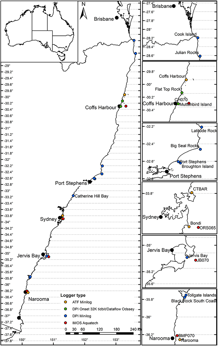
Figure 1. Study site map showing the location of each in situ mooring and logger. Horizontal lines indicate the 0.20° of latitude that is used to average the data in the remaining figures.

Datasets

In situ IMOS Mooring Data

In situ water temperature was collected by the NSW-Integrated Marine Observing System (IMOS) mooring team (Roughan and Morris, 2011; Roughan et al., 2015) and was obtained from the IMOS Data Portal (https://portal.aodn.org.au) for four moorings (CH070, ORS065, JB070, and BMP070) deployed at latitudes between ~ 30° to 36°S (Table 1, red dots on Figure 1). In addition to measuring current velocity (not used here), each mooring consisted of a line of thermistors (Aquatech 520 temperature and temperature/pressure loggers; resolution ±0.05°C) at 4-m (ORS065 only) or 8-m intervals through the water column extending from the bottom to a sub-surface float (15–20 m below the surface; see Roughan et al., 2015 for full details of the mooring configuration). All data were logged internally at 5 min intervals and downloaded at servicing every 8–12 weeks. The depth of the thermocline was calculated for each mooring location (per 5 min intervals) by determining the largest temperature difference across the string of temperature loggers (from minimum depth to 45 m). If a temperature difference between the shallowest depths was evident and constant, the thermocline was assumed to coincide with the minimum depth, i.e. no mixed layer. All depths within or below the thermocline were excluded as this water mass would be decoupled from the shallower waters. The minimum thermocline depth was 19 m (mean 37 m). Data were collected between 2006 and 2017, however the temporal period of available data differed between each mooring and depth, with data coverage ranging from 94 to 3,676 days per mooring/depth (Table 1).

TABLE 1

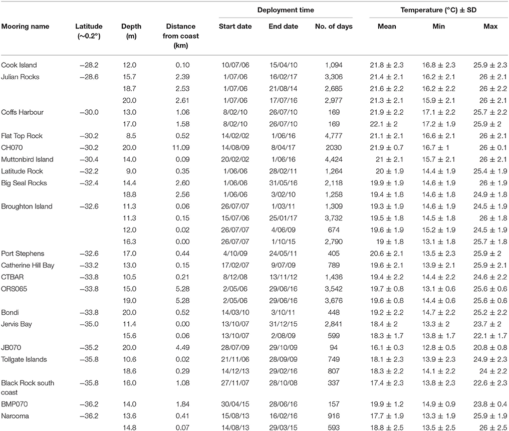
Table 1. Table of in situ IMOS moorings and NSW DPI-Fisheries loggers included in study given from north to south with deployment dates, number of days with data available, mean, minimum and maximum temperatures recorded by site and depth.

In situ NSW DPI-Fisheries Logger Data

NSW DPI-Fisheries and the IMOS Animal Tracking Facility (IMOS-ATF) (hereafter collectively referred to as “NSW DPI-Fisheries” loggers) deployed in situ temperature loggers at 16 sites (Figure 1), with a total of 26 loggers (Table 1). Data were collected for different periods of time at each deployment location (Table 2). Two models of Minilog Temperature Data Loggers (Vemco - Amirix Systems Inc., Halifax, Canada) were deployed by NSW DPI-Fisheries at nine of the 16 sites from 2006 to the present. Each logger was deployed approximately 1 m above the seabed together with a passive acoustic listening station (Otway and Ellis, 2011). Initially, Minilog 8TR loggers were used (2006–2010) and recorded the water temperature once every 60 min. These loggers were later replaced with Minilog II-T loggers (2011 to present), which also recorded water temperature once every 60 min. Both loggers had a resolution of 0.01°C, were accurate to ±0.10°C and deployed for periods of up to 12 months with retrieval and re-deployment done by scuba divers.

TABLE 2

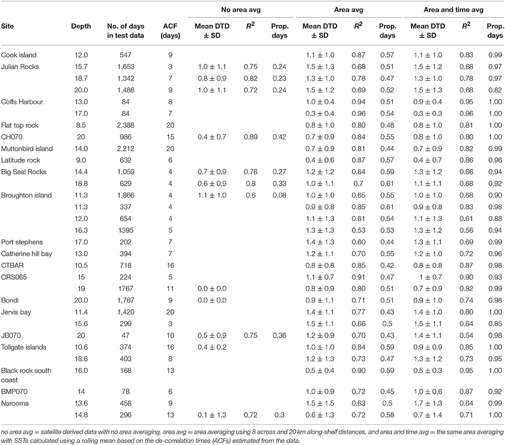
Table 2. Table of data obtained from in situ IMOS moorings and NSW DPI-Fisheries loggers given from north to south with de-correlation times (ACF, days), mean daily temperature difference (daily satellite SST minus in situ temperature- DTD), R² values from linear regressions against the in situ data and proportion of study days (prop days) with corresponding satellite data.

IMOS-ATF also deployed Minilog II-T loggers at Coffs Harbour, Port Stephens, Sydney (Manly, and Bondi) and Narooma (Figure 1). Like the NSW DPI-Fisheries instruments, loggers were deployed approximately 1 meter above the seabed on passive acoustic listening stations and retrieved every 12 months.

At Muttonbird Island and Flat Top Point (Figure 1) Onset 32 K TidbiT loggers (Onset Computer Corporation, MA, USA; resolution 0.16°C) were used from 2001 to 2006. Dataflow Odyssey loggers (Dataflow Systems Ltd, New Zealand; resolution 0.02°C) were used from 2006 to 2011, Reefnet Sensus loggers from 2011 to 2014, and thereafter Onset Hobo Pro V2 loggers. Loggers were accurate to within 0.16°C from trial comparisons (Malcolm et al., 2011). All loggers were deployed for up to 12 months and recorded the water temperature every 30 min.

Any data from loggers that were deployed deeper than the estimated thermocline depth (calculated from data at the mooring deployed closest to the logger location) were excluded. For example, if the thermocline was estimated to be at 19 m for a particular mooring then all loggers deployed in the vicinity of that mooring and at depths >19 m were excluded.

Satellite Derived SST

Daily day-night composites (L3S product) of satellite-derived SST foundation (~10 m depth) measurements obtained by the advanced very high resolution radiometer (AVHRR) aboard the NOAA series of satellites were accessed from the IMOS Ocean Portal (https://portal.aodn.org.au) (Imos, 2017). SST foundation was used instead of skin-SST (~10–20 μm water depth) as it is largely free of diurnal temperature variability (Beggs et al., 2011). As part of routine data processing, IMOS calculate SST from multiple sensors at a spatial resolution of 0.02° latitude × 0.02° longitude (Beggs et al., 2010). Each gridded cell contains the average of all the highest available quality SSTs that overlap with this cell, weighted by area of overlap (Beggs et al., 2010). These data are then flagged according to bias (median bias over all measurements over the time window of consideration- “sses bias” variable field in the data) and data quality (based on relationship to land, atmospheric quality and the distance to the nearest cloud—“l2_flag” and “quality_level” variable fields in the data—Griffin et al., 2017). We subtracted the sses bias from the L3S SST measurements (as recommended by http://imos.org.au/facilities/srs/sstproducts/sstdata0/reading-data/) and filtered according to the data quality so that only “acceptable” or “best” quality (quality level ≥ 4) data were used. Thus the SST data subsequently used in this paper did not include any data close to clouds (>5 km) or land, and thus were not available for all the same dates as the in situ measurements.

Data Analysis

Differences Between in situ and Satellite-Derived SST

Temperatures from all the in situ loggers were used to describe the thermal environment across the different latitudes and depths of our study locations (daily mean and range averaged across each month, annual maxima and minima). The daily temperature mean and range (maximum minus minimum temperature) were calculated for each logger and averaged across all the locations within 0.20° latitudes (~20 km along-shore to match the distances used in the area averaging, see below, and within temperature decorrelation lengths- Schaeffer et al., 2016) and within 2 m depth intervals (8–9.9, 10–11.9, 12–13.9, 14–15.9, 16–17.9, and 18–20.0 m) for each month. Data were not differentiated by across-shelf distances as all sites were less than the known decorrelation length scales, even at depth (all sites were ≤ 11.09 km offshore; decorrelation length scales: 19 km on the surface and 14 km at 50 m depth- Schaeffer et al., 2016).

The data from each in situ logger were split into two independent datasets representing two different temporal periods: (1) 50% of the data from the first deployment was used as a “training” dataset to calculate the daily temperature difference and find the “optimal” across- and along-shelf distances (see below); (2) the remaining 50% of the data, the “test” data, was used to validate the correction methods using decorrelation length- and time-scales. To determine the differences between the in situ and satellite data, the daily mean was calculated for each in situ logger locations in the training dataset to match the temporal resolution of the satellite-derived data. Each in situ recording was matched to a corresponding satellite SST measurement extracted from the satellite pixel directly over the sampling location (hereafter referred to as “no area averaging”). Daily temperature differences (daily satellite SST minus in situ temperature, hereafter DTD) were calculated to examine short term and seasonal variation in differences between in situ and satellite measurements, in a manner synonymous with Stobart et al. (2016). These matchups were used to compare the average DTDs for each month for each 0.20° latitudinal range and depth interval.

Using De-Correlation Length Scales from in situ Data to Inform Area- Averaging of SSTs

The EAC flow is typically anisotropic, meaning the flow dominates in one direction, in this case along-shore to the south (poleward). Schaeffer et al. (2016) determined that the mean temperature de-correlation length scales at a latitude of ~29.5–33.0°S, upstream of the EAC separation point, were 19 and 29 km in the across- and along- shelf directions in the surface mixed layer. The across-shelf (along-shelf) distances decreased (increased) with increasing water depth. Varying across- and along-shelf distances were used to area average the satellite derived SST measurements. Across-shelf distances of 4–20 km (increments of 2 km, which is approximately the resolution of the satellite pixels) and along-shelf distances of 5–45 km (increments of 5 km) were used to calculate the area-averaged estimate of SST. Across-shelf distances were extended offshore from the in situ location while along-shelf distances were centered on the latitude of the in situ logger. The mean across all the satellite pixels were used as the satellite derived SST measurement as shown below:

$\begin{array}{l}SS{T}_{areaavg}=\frac{1}{n}\times {\displaystyle \sum _{i,j=1}^n}{x}_{ij}\end{array}$

where i = latitude coordinate of the in situ logger ± 0.5*the along-shelf distance (4–20 km were tested), j = longitude coordinate + the across-shelf distance (5–45 km were tested) and n = the total number of satellite pixels in the i and j distances. Note: j is positive in this study so that the distance extends offshore; this would be negative along a western coastline. The output (SST_areaavg) is a single value for each in situ location for each day.

The “optimal” across- and along-shelf distances to use were assessed from the differences between in situ (from the training dataset) and satellite data, and the correlation (Pearson's correlation) between the two measurements. The daily area averaged SST value from the “optimal” across- and along-shelf distances (8 and 20 km respectively- see section Results) were then compared to the corresponding in situ test data using a linear regression to determine if there was a statistically significant difference between the two measurements.

Gap Filling Using De-Correlation Times Scales

Generally temperature in the mesoscale ocean changes fairly slowly (far less quickly than say diurnal temperature changes in the atmosphere over land). Roughan et al. (2015) found that the de-correlation times of oceanic temperature (including the same IMOS mooring data that is included in this paper) vary from 2.3 to 20 days (in 98 to ~10 m water depth, respectively). Autocorrelation functions (ACF) were used to determine the sea temperature de-correlation times using the in situ test data from all locations and the methods of Roughan et al. (2015). The hourly mean temperature for each in situ location was calculated for periods of time when there were no gaps in the logger data and the de-correlation time was taken as the maximum lag with an ACF greater than 0.7. These de-correlation times, along with across- and along-shelf distances of 8 and 20 km respectively, were then used to calculate a rolling mean SST (centered on the day of interest) from the satellite derived data to fill gaps when data was filtered out due to poor data quality flags (e.g., there was cloud cover) as shown in equation below.

$\begin{array}{l}SS{T}_{areaandtimeavg}=\frac{1}{n}\times {\displaystyle \sum _{i,j,k=1}^n}{x}_{ijk}\end{array}$

where i = latitude coordinate of the in situ logger ± 0.5*the along-shelf distance, j = longitude coordinate + the across-shelf distance, k = date of in situ logger recording ±0.5*the de-correlation time (as calculated by ACF) and n = the total number of satellite pixels in the i and j distances over k time. Note: j is positive in this study so that the distance extends offshore; this would be negative along a western coastline. Again, the output (SST_{area and time avg}) is a single value for each in situ location for each day.

The total number of days before and after the gap filling and DTDs were calculated. Again, a linear regression was used to compare the single daily area- and time- averaged SST value with the corresponding in situ test data.

Comparison of Satellite Processing Methods

Pairwise (paired) t-tests were used to compare the SST measurements per location (i.e., the location of the in situ loggers) from each of the three satellite processing methods [no area averaging, area averaging (using across- and along-shelf distances) and area- and time- averaging [using the rolling mean to input missing days in the satellite data]) to determine if there was any significant difference between the methods. In addition, t-tests were used to determine if there was an overall difference between the SST measurements from each method across all locations and for each depth interval. Similarly, Wilcoxon tests were used to determine if there was an overall difference in the R² values and proportion of days from each method across all locations and for each depth interval. Wilcoxon tests were used for the latter as the data was non-normally distributed.

A linear mixed model (LMM) was used to determine the influence of the satellite processing method, depth, latitude, and distances to estuary and coast on the DTDs (response variable). The unique site name was used as a random effect to account for the repeated measures on the same site (Zuur et al., 2009). The full equation for the LMM is shown below:

$\begin{array}{l}DT{D}_{ij}~\alpha +sa{t}_{ij}+{\beta }_{1}dept{h}_{ij}+{\beta }_{2}la{t}_{ij}+{\beta }_{3}es{t}_{ij}+{\beta }_{4}coas{t}_{ij}\\ +a_j+{\epsilon }_{ij}\end{array}$

where sat is the method used to process the satellite data; lat is latitude; est is the distance to estuary; coast is the distance to the coast; α is the random intercept for each in situ logger (indexed by j) for each day (indexed by i), while the ε is a Gaussian error term.

The LMM was implemented using the lme4 R package (Bates et al., 2014). Prior to modeling, data exploration was conducted following the general protocol of Zuur et al. (2010) using Cleveland dot plots, boxplots, and scatterplots to identify patterns and any outliers. A variance inflation factor (VIF) was used to determine if the explanatory variables were correlated and no co-linearity was evident (all VIF values < 3). Model selection for the best model was based on the Akaike Information Criterion (AIC). Any models with a difference in AIC (ΔAIC) of less than or equal to two had “strong support”; ΔAIC of four to seven showed “substantial support” and ΔAIC greater than 10 showed “no support” (Burnham and Anderson, 2002). If more than one model had ΔAIC of 10 or less, model averaging was used to calculate the variable coefficients (Bolker et al., 2009) and relative importance of each variable using the MuMIn R package (Barton, 2012). The relative importance is the sum of the AIC weights across all the models with a ΔAIC of 10 or less that contain the explanatory variable.

Results

In situ Temperature

Annual mean temperatures at the in situ locations ranged from 16.1 to 22.1°C (Table 1). Annual mean and minimum temperatures decreased polewards, while maximum temperatures were approximately 26°C from the northern most part of the study area (28°S) to 33°S and then decreased with increasing latitude (Table 1). The mean temperatures showed clear seasonal patterns across each of the different latitudes included in this study (Figure 2). Similar temperatures were recorded for the different depths (8–20 m) at each latitude (Figure 2). The daily temperature ranges averaged for each month and 0.20° latitude also showed clear seasonal patterns with larger temperature ranges at the start of the year (Figure 3) with average daily temperature fluctuations of 1.21°C (and up to 4.20°C). Temperature ranges were smallest in the austral winter months with the smallest short-term fluctuations in June–August (months 6–8 on Figure 3; mean seasonal temperature ranges: summer: 2.04°C, autumn: 1.12°C, winter: 0.56°C, and spring: 1.18°C).

FIGURE 2

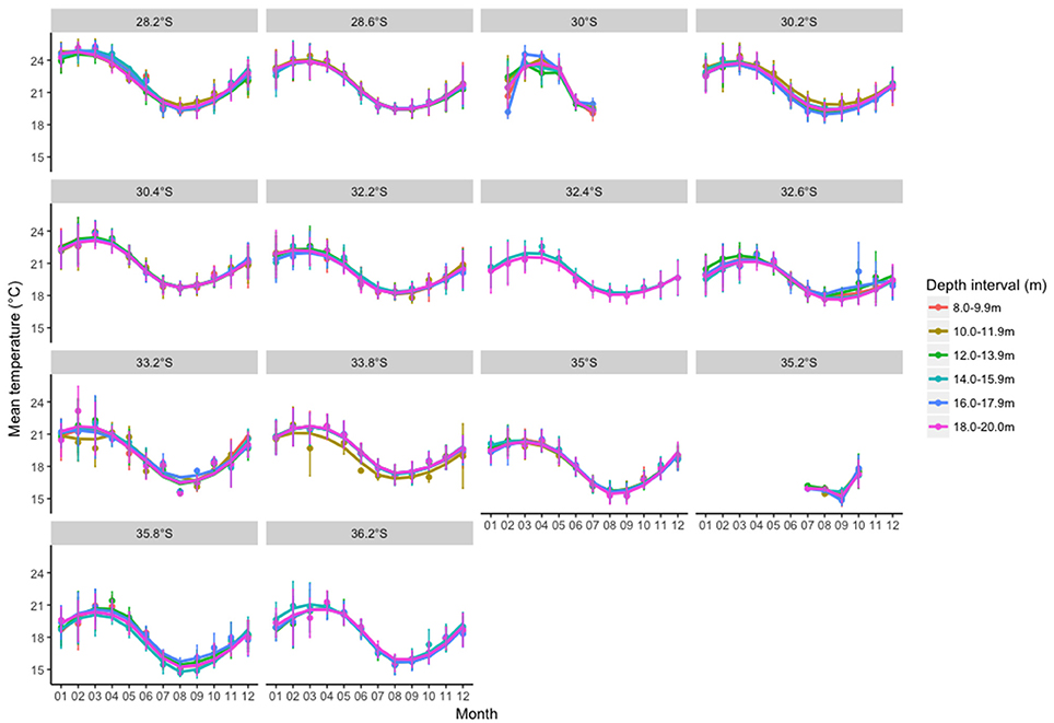
Figure 2. Mean monthly temperatures for in situ locations across each 0.20° latitude and 10 m depth intervals.

FIGURE 3

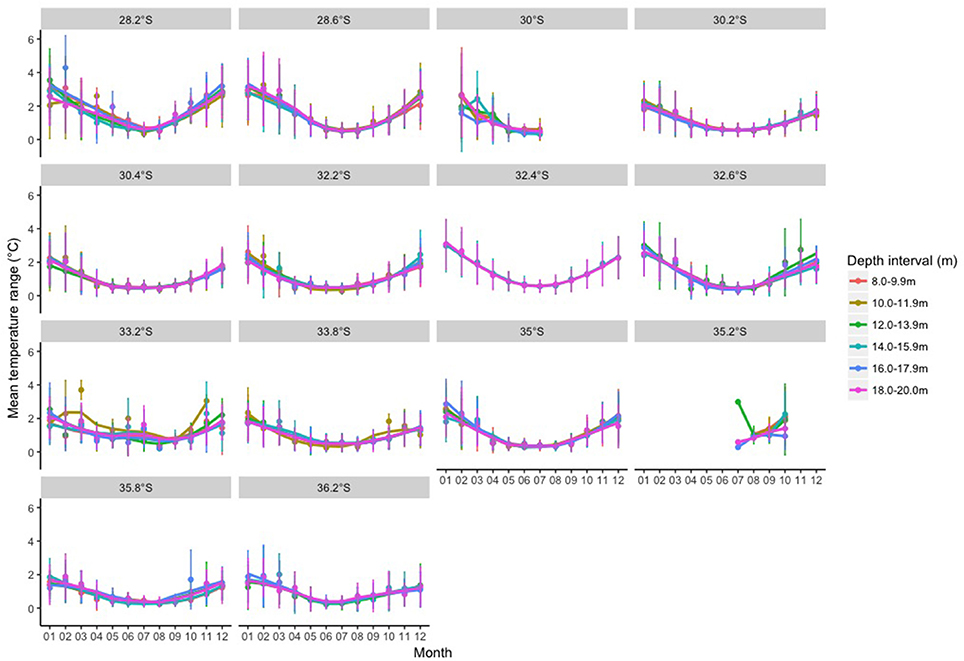
Figure 3. Mean monthly temperature ranges (averaged from daily ranges) for in situ locations across each 0.20° latitude and 10 m depth intervals.

Assessing Across- and Along-Shelf Distances to Inform Area- Averaging of SSTs

The correlation between in situ and satellite derived sea temperatures was variable depending on the across-shelf distance used to area average the satellite values (Figure 4). The correlation decreased with increasing across shelf distances used for the area averaging for all of the latitudes and depths, albeit at different rates (Figure 4), except for 12–13.9 and 16–17.9 m at 30.0°S, which increased from 4 to ~12 km before decreasing or plateauing across the remaining distances. Moreover, correlations were greatest at highest and lowest latitudes and shallower depths (e.g., correlations were > 0.75 at 28.2 and 35.8°S, and greater at 10–11.9 m vs. ≥12 m at 33.8°S or 12–13.9 vs. 16–17.9 m at 30.0 and 35.0°S). The only exception to the latter was at 35.8°S where the correlations at 16–17.9 m were less than at 18–20 m (Figure 4). The proportion of days that the in situ loggers had corresponding satellite values increased as the across-shelf distances used in the area averaging increased (Figure 5). Thus, taking into account the relative change in correlation for different across shelf distances and proportion of days with satellite data, an across-shelf distance of 8 km was used for the remaining analyses. This is approximately half the known across-shelf de-correlation length scale estimated for surface waters upstream of the EAC separation zone (Schaeffer et al., 2016).

FIGURE 4

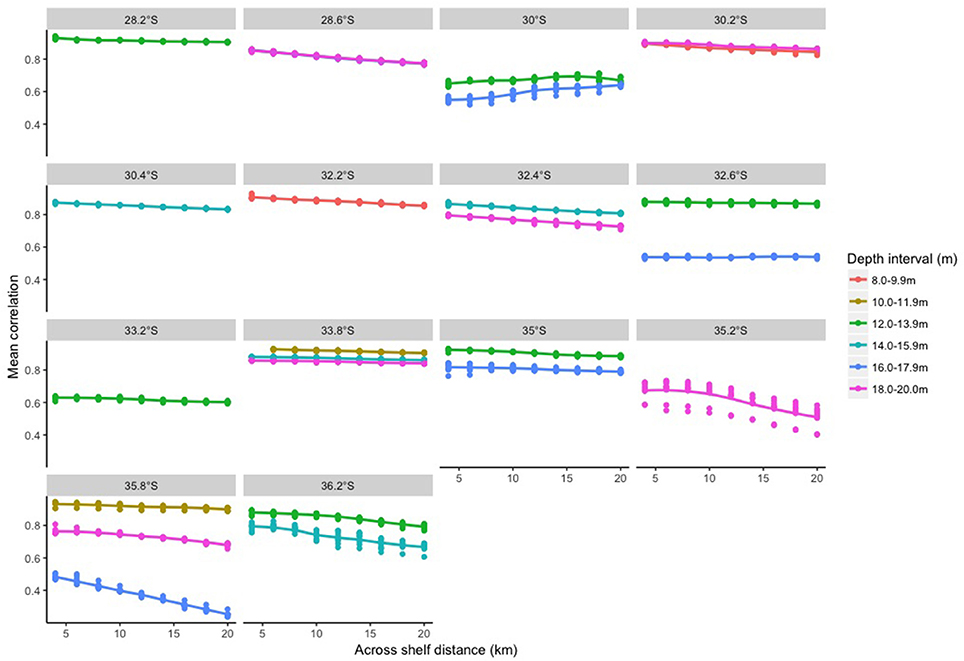
Figure 4. Mean Pearson's correlation between satellite data and in situ data for different across-shelf distances.

FIGURE 5

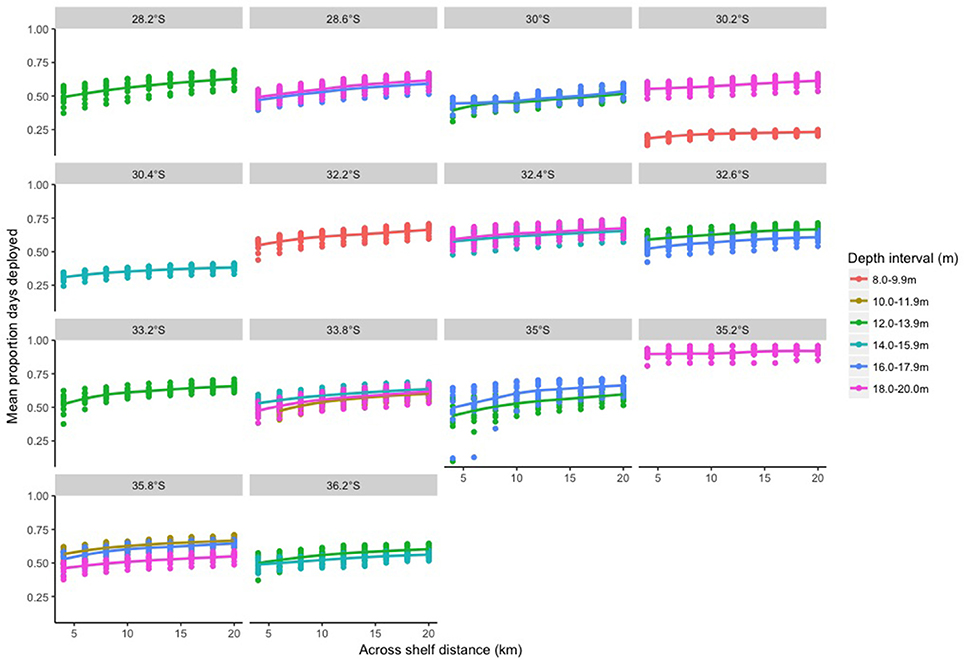
Figure 5. Mean proportion of days that loggers were deployed that had corresponding satellite data for different across-shelf distances.

The along-shelf distances used in the area averaging had less of an effect on the correlations than the across-shelf distances (Figure 6). For many of the latitudes and depths, increasing the along-shelf distance used in the area averaging did not alter the correlations (e.g., all correlations at 28.2°S were ~0.90 and all depths at 33.8°S remained constant). In contrast, the correlation of the in situ data and the satellite derived data decreased from ~0.75 to ~ 0.66 with along-shelf distances of 5–20 km at 30.0°S and 16–17.9 m depth while it increased over the same distances for temperatures from 18 to 20 m at 35.2°S, and 12–13.9 m at 36.2°S. The proportion of days with corresponding satellite values also increased with larger along-shelf distances used in the area averaging (Figure 7). Overall, the average correlation values remained the same (0.78) and the mean proportion of days with corresponding satellite data across all the sites increased from 0.47 to 0.54 with along-shelf distances of 5 and 20 km. Thus, an along-shelf distance of 20 km was used for the remaining analyses, which is within the range of known along-shelf de-correlation distances of 29 km for surface waters (Schaeffer et al., 2016).

FIGURE 6

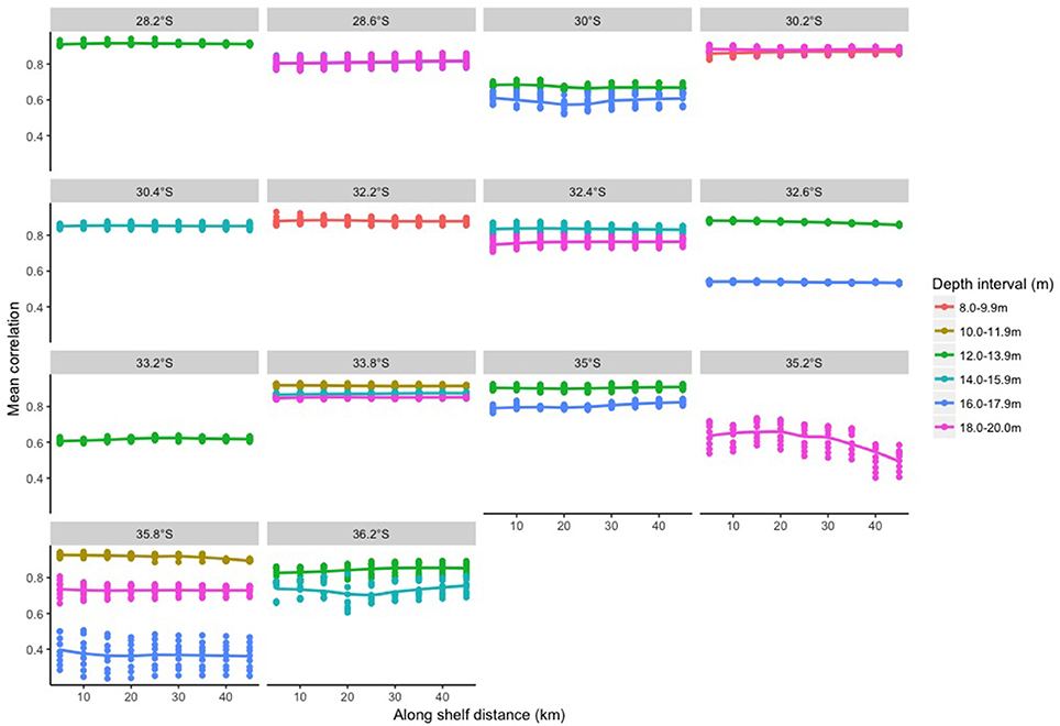
Figure 6. Mean Pearson's correlation between satellite data and in situ data for different along-shelf distances.

FIGURE 7

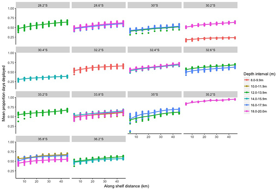
Figure 7. Mean proportion of days that loggers were deployed that had corresponding satellite data for different along-shelf distances.

De-Correlation Time Scales

De-correlation times varied between 3 and 20 days at the in situ locations (Table 2) with no clear pattern evident between latitudes. However, data from the deeper moorings showed a decreasing de-correlation time with increasing water depth (Table 2) in agreement with Roughan et al. (2013, 2015).

Differences Between in situ and Satellite Temperatures

Satellite SST foundation temperatures obtained directly over the sampling locations (i.e., no area averaging) were only 39% of the sites (12 out of 31; Table 2). For these sites, the satellite SSTs were significantly different from the in situ measurements except for at 10–11.9 m depth (Table 3). However, all the satellite derived values (except for no area-averaging at 10–11.9 m depth) were significantly different from the in situ measurements, regardless of how the data were processed (Table 3). Nevertheless, using the area averaging and the area- and time- averaging methods increased the overall proportion of days compared to no area averaging (Table 3), although there was only significant increase overall and between the area and area- and time-averaging methods (Table 3).

TABLE 3

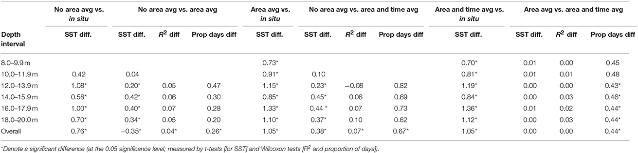
Table 3. Table showing the pairwise comparisons of the different satellite processing methods, including mean differences in SST (SST diff) between the different methods and the in situ data, R² (R² diff) and proportion of days with satellite measurements (prop days diff) per depth interval and for all locations (overall).

For the sites where satellite SST foundation data was available for the no area averaging, only 27% of the study days had corresponding satellite measurements (Table 2). However, using the area averaging significantly increased the number of days to 52%, while using both the area- and time-averaging approach overall increased this to 96% (values for each site given in Tables 2, 3 for value per depth and all sites combined). Unsurprisingly, as the de-correlation time for a particular site increased so did the proportion of days that data could be filled in using the time-averaging (rolling mean) method (Table 2).

The mean DTD per site for satellite data with no area averaging ranged from 0.11 to 1.08°C, which was lower than the satellite data with area averaging (0.28 to 1.50°C) and area averaging with a rolling mean (0.30 to 1.70°C; Table 2). Both the area and area- and time-averaged methods were significantly different to the no area averaging approach except for at 10–11.9 m, but there was no difference between the two area averaging methods (Table 3). The mean DTD per month varied greatly over the year for all satellite data processing methods (Figures 8–10), with the highest DTDs corresponding to the months with the highest daily temperature ranges (Figure 3). The DTDs were similar over the different latitudes but increased with increasing water depth (Figures 8–10).

FIGURE 8

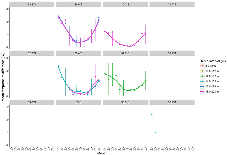
Figure 8. Mean temperature differences between in situ and satellite that was processed at each logger location (i.e. no area averaging).

FIGURE 9

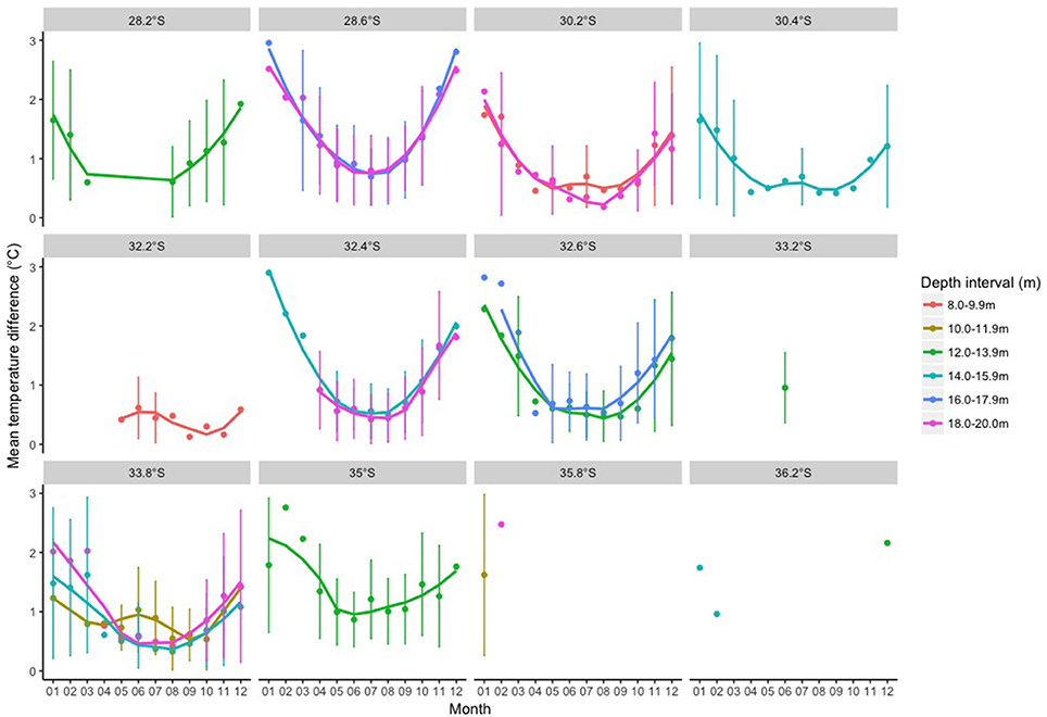
Figure 9. Mean temperature differences between in situ and satellite that was processed at each logger location using an area average of 8 km across shelf and 20 km along shelf (i.e. area averaged values).

FIGURE 10

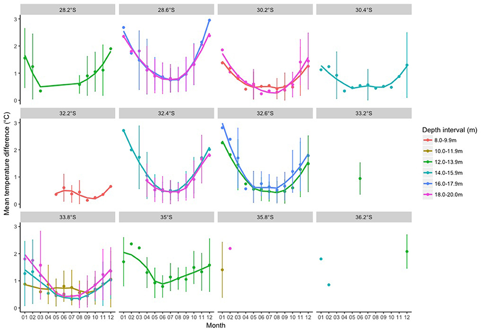
Figure 10. Mean temperature differences between in situ and satellite that was processed at each logger location using an area average of 8 km across shelf and 20 km along shelf with a rolling mean based on the de-correlation time for the in situ location to fill in missing data (i.e. area- and time- averaged values).

Model selection of the LMM produced eight model candidates with a ΔAIC of 10 or less (Table 4). Model averaging showed that satellite data processing method and depth were the most important variables influencing DTDs (both had relative importance [rel. imp.] of 1.00). This was followed by distance to estuary (rel. imp. 0.78), distance to coast (rel. imp. 0.34) and, lastly, latitude (rel. imp. 0.28). DTDs were significantly larger for the area averaging and area averaging with rolling mean methods of processing the satellite data compared to no area averaging (Table 5). The DTDs significantly increased with increasing depth (Table 5) and, although DTDs decreased with increasing distance from the nearest estuary, from the coast and latitude (i.e., north to south), these differences were not significant.

TABLE 4

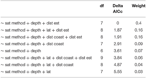
Table 4. Table of the most parsimonious linear mixed models (all models with ΔAIC ≤ 10). df, the degrees of freedom.

TABLE 5

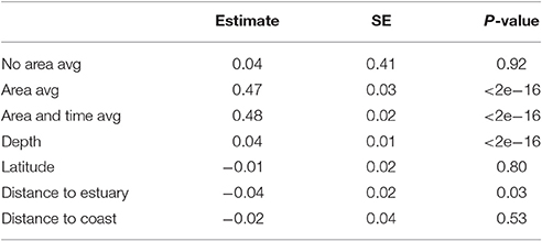
Table 5. Table of the model averaged estimates, standard errors (SE) and p-values from all the most parsimonious linear mixed models.

Discussion

This study demonstrates that using well-chosen area averaged satellite SST data can increase the likelihood of obtaining an SST measurement for coastal areas. Only 39% of sites had satellite data directly over the logger locations for ~27% of the study time. In contrast, area averaged satellite SST data was available for all sites 52% of the study time, which increased to 96% when also incorporating a time-averaged component (rolling mean) based on de-correlation times to impute missing data. Although the differences between in situ and satellite SST foundation temperature data were larger for area averaged measurements, the difference in temperature measurements was only on average 1.05°C and less than the maximum daily temperature fluctuations observed in situ (Figure 3). Therefore, known across- and along-shelf de-correlation lengths can be used to inform how many satellite pixels should be used to obtain an appropriate area averaged SST. In addition the de-correlation time scales (estimated from the in situ temperature data) can be used to gap fill the satellite derived temperature record for days when no satellite data are available (e.g., too much cloud cover). Together, these two methods can increase the total number of days for which satellite data are available for a sampling location (Figures 5, 7; Tables 2, 3), thus reducing the effect of missing data on studies.

Seasonal Temperature Cycle

As shown in Figure 2, the in situ temperature exhibited a clear seasonal cycle, with highest mean temperatures in the late austral summer/early autumn (March to April; months 3–4) and lowest in late winter/early spring (August/September; months 8/9). This pattern was evident across all latitudes, however the mean temperature peaked in April (month 4) rather than March (month 3) for sites further south. Seasonal vertical temperature stratification is due to local wind forcing driving upwelling during the summer months and mixing during the winter months (Wood et al., 2016). This also influenced the seasonal in situ daily temperature ranges (averaged across each month) observed in this study (Figure 3). In situ daily temperature ranges were greatest (up to 4.20°C) in the austral summer and early autumn months (January to March- months 1–3 on Figure 3), which corresponded with the strongest vertical temperature stratification (Wood et al., 2016). These larger daily temperature fluctuations in the summer and early autumn in turn correlated with greater differences between the in situ and satellite temperatures (Figures 8–10).

Correlations Between in situ vs. Satellite-Derived Temperatures

The findings of this study are consistent with previous studies that have compared in situ temperature data from intertidal (Lathlean et al., 2011), subsurface (Pearce et al., 2006), and shallow waters (Smale and Wernberg, 2009; Stobart et al., 2016) with satellite SST data. However, all of these studies used either the closest satellite pixel to their study location (Malcolm et al., 2011; Baldock et al., 2014), an average of all the satellite data within an arbitrary distance (e.g., 20 km² box centered on logger location: Stobart et al., 2016), or number of pixels (Delgado et al., 2014) from the logger locations. This study demonstrates how the choice of the number of satellite pixels used in across- and along-shelf directions affect the correlation of the data to in situ measurements. As the EAC flow is typically anisotropic (dominant along-shore flow), the choice of the number of satellite pixels used in the alongshore direction had less of an effect on the correlations than number of pixels used in the across shore direction.

Correlations between the in situ and satellite data were greater upstream and downstream of the EAC separation zone (i.e., greatest at higher and lower latitudes). Although the EAC separation zone can occur anywhere between 28° and 38°S, it predominately occurs at 30.7°-32.4°S (Cetina Heredia et al., 2014). Across- and along-shelf correlations at 20–29 m depth decreased by ~0.06 at latitudes within the separation zone (32.2° and 32.4°S respectively; Figures 4, 6) compared to the latitudes immediately north (30.4°S: decrease of 0.03) and south (32.6°S: decrease of 0.01). Mesoscale eddies regulate the temporal variability in the EAC separation zone, with a southward progression as eddies develop and then an abrupt retraction in latitude after the detachment of an eddy (Cetina Heredia et al., 2014). These eddies may be warm core (anti-cylonic) or cold core (cyclonic), with deep or shallow mixed layer depths respectively. Thus the area within and south of the separation zone has increased anomalies of sea level, surface temperature and surface chlorophyll a (Everett et al., 2012, 2014) resulting in a highly dynamic area in which temperatures change over shorter across-shelf distances and depths. This is particularly evident at 35.8°S where there was a larger difference between the correlation between in situ and satellite data (against different across-shelf distances) at different depths other latitudes (Figure 4).

Even with the lower correlations within the EAC separation zone, the correlations between in situ and satellite data were ≥0.73 in water depths of 8–16 m within all across- and along-shelf distances tested in this study. This indicates that satellite SST foundation temperatures (~10 m water depth) can be used as a proxy for water depths < 16 m but must be used with caution for deeper waters, as correlations decreased to ≤ 0.66. Therefore, long-term in situ monitoring is needed for water depths >16 m, as this is information that is not available from satellite data. It has been shown that extreme marine temperature events (e.g., marine heatwaves: Schaeffer and Roughan, 2017) can occur throughout the water column, and their intensity and duration may be either not detected or underestimated by satellite SST. Such events can have devastating consequences on marine biota (Smale and Wernberg, 2012; Wernberg et al., 2013). Without long-term national monitoring locations, such as the Australian National Reference Station network, which provide sub-surface temperature information (Lynch et al., 2014), the frequency and severity of such events may be underestimated and thus omitted from marine management strategies.

Latitude, distance to the coast and nearest estuary did not influence the difference between the in situ and satellite data as much as the water depth. A number of the loggers used in this study were deployed close to marine/tide dominated estuaries (e.g., Jervis Bay) with low and intermittent freshwater inflows (and thus shallow intermittent river plumes, e.g., Johnston et al., 2015). This is in agreement with Stobart et al. (2016), who also found that the proximity to estuaries did not explain differences between in situ and satellite data in the vicinity of low flow/tide-dominated estuaries. Thus in proximity to low flow estuaries, ocean dynamics (which manifest as temperature changes at depth, latitude and season) play a greater role in influencing temperature (and thus biases in satellite derived data).

Area Averaging and Gap Filling Satellite Data

It was only possible to extract satellite data directly over the sampling locations for 12 out of the 31 sites included in this study due to their proximity to the coast. Therefore, although the difference between the in situ and satellite data increased when using an area averaging approach, data were available for all sites and a longer proportion of the study time. In addition, the overall temperature differences between the in situ and satellite data only increased by ~0.29°C, which was substantially less than the mean daily temperature ranges of up to 1.21°C (and maximum of up to 4.20°C) experienced in the austral summer/early autumn. Although this approach allowed more sites close to the coast to be sampled, up to 57% of the time satellite data were still missing (due to cloud cover). Complex, multivariate approaches can be used to interpolate missing data [e.g., the Data Interpolating Empirical Orthogonal Functions (DINEOF)- (Alvera-Azcárate et al., 2007)], however here we showed that using a rolling mean based on the de-correlation time of each site produced data on average for 96% of the study time, while changes in the differences between the in situ data were minimal. The combined area averaging and use of a rolling mean (i.e., the area- and time-averaged method) provides researchers working in coastal areas with simple method by which SST data can be extracted for stationary, point locations. Future studies using satellite data as a proxy for in situ temperatures should consider the dominant oceanographic conditions of their study site, preferably using known de-correlation length and time scales (such as those quantified by Schaeffer et al., 2016 and Roughan et al., 2015, repsectively), to determine the appropriate number of satellite pixels for obtaining their SST measurements and the number of days over which to average. However, users should be aware that SST measurements from polar-orbiting satellites (even with no area averaging) may be significantly different from in situ measurements and may not capture the full seasonal variability in short-term changes in temperature (such as the daily temperature ranges observed from the in situ data in this study). Such areas may be of high biological or ecological importance (Scales et al., 2014), thus the suitability of using SST as a proxy for in-water temperature will depend on localized conditions and specific temperature value of interest (e.g., weekly SST versus identifying “frontal” systems). For example, satellite derived measurements (regardless of whether they are area- and/or time-averaged) will not be able to capture the full variability in the ranges of temperatures experienced over short time scales (of hours rather than days) within the dynamic EAC separation zone, where, as previously discussed, warm- and cold-core eddies regularly detach from the EAC poleward flowing jet (Cetina Heredia et al., 2014). Likewise, satellites will not detect upwellings or marine heatwaves that do not reach the surface. In both of these examples the use of an area- (and time-) averaging approach may further reduce the ability to truly represent these short-term changes, as the measurements will be representative over a wider spatial area (and temporal period).

Implications for Future Research

Studies using satellite SST to determine the influence of seasonal water temperature should be aware of the seasonal biases and differences with in situ data. In addition, satellite data may not reflect the full range of temperature variation that may be ecologically important for marine biota, particularly at short-term scales and at depth. This sentiment reflects that of previous research, whereby Smale and Wernberg (2009) concluded that satellite SST data do not “adequately detect ecologically important small-scale variability or provide reliable information on temperature extremes” and Stobart et al. (2016), who highlighted that SST was only reliable for broad temperature patterns. These, together with increasing frequency of extreme temperature events (e.g., marine heatwaves; Schaeffer and Roughan, 2017), makes long-term monitoring programs critical especially those that provide high resolution temperature over a range of spatial scales (including depth).

In conclusion, our results show that de-correlation length and time scales can be used to process satellite data to overcome coastal contamination and missing data, however, care must be taken when using such data and the suitability should be assessed on a case-by-case basis. The correlation between satellite derived SST and in situ data is dependent on the latitude, depth of data acquisition and the time of year. Local oceanographic and weather conditions will differentially affect water temperatures through the water column and over shorter temporal scales than satellite data are measured. However, our results show that with careful consideration of the above factors, satellite derived SST can be used as a proxy for temperature in the top 15 m along the coast of SE Australia, in a highly dynamic WBC regime.

Author Contributions

NO, HM, and MR all provided in situ temperature data. KL analyzed all the data, sourced the satellite-derived data and wrote the manuscript, with all other authors contributing to editing the drafts.

Conflict of Interest Statement

MR held joint appointments at UNSW Australia and MetOcean Solutions Ltd (New Zealand MetService Group).

The remaining authors declare that the research was conducted in the absence of any commercial or financial relationships that could be construed as a potential conflict of interest.

Acknowledgments

MR held joint appointments at UNSW Australia and MetOcean Solutions Ltd. (New Zealand MetService Group). All other authors declare no competing interests. Oceanographic data were sourced from the Integrated Marine Observing System (IMOS), – IMOS is a national collaborative research infrastructure, supported by the Australian Government. Data from the ocean reference station (ORS065) were provided by Sydney Water Corporation. KL was partly supported by a Research Attraction and Acceleration Program (RAAP) from the NSW Office of Science and Research and administered through the NSW State and Revenue. We specially thank Brett Louden and the technicians and contractors working with NSW DPI-Fisheries and NSW-IMOS for assisting in the collection of the in situ data. We also thank the two reviewers for their comments that helped improve this manuscript.

References

Allan, B. J., Domenici, P., Munday, P. L., and Mccormick, M. I. (2015). Feeling the heat: the effect of acute temperature changes on predator–prey interactions in coral reef fish. Conserv. Physiol. 3:cov011. doi: 10.1093/conphys/cov011

PubMed Abstract | CrossRef Full Text | Google Scholar

Alvera-Azcárate, A., Barth, A., Beckers, J. M., and Weisberg, R. H. (2007). Multivariate reconstruction of missing data in sea surface temperature, chlorophyll, and wind satellite fields. J. Geophys. Res. Oceans 112:C03008. doi: 10.1029/2006JC003660

CrossRef Full Text | Google Scholar

Baldock, J., Bancroft, K. P., Williams, M., Shedrawi, G., and Field, S. (2014). Accurately estimating local water temperature from remotely sensed satellite sea surface temperature: a near real-time monitoring tool for marine protected areas. Ocean Coastal Manag. 96, 73–81. doi: 10.1016/j.ocecoaman.2014.05.007

CrossRef Full Text | Google Scholar

Barton, K. (2012). MuMIn: Multi-Model Inference. R Package Version 1.7.7. Available online at: http://CRAN.R-project.org/package=MuMIn

Bates, D., Maechler, M., Bolker, B., and Walker, S. (2014). lme4: Linear Mixed-Effects Models Using Eigen and S4. R package Version 1.1-7. Available online at: http://CRAN.R-project.org/package=lme4

Beggs, H., Majewski, L., Paltoglou, G., Schulz, E., Barton, I., and Verein, R. (2010). “Report to GHRSST11 from Australia–BLUElink and IMOS,” in Proceedings of the 11th GHRSST Science Team Meeting (Lima), 21–25.

Google Scholar

Beggs, H., Zhong, A., Warren, G., Alves, O., Brassington, G., and Pugh, T. (2011). RAMSSA—an operational, high-resolution, regional australian multi-sensor sea surface temperature analysis over the Australian region. Aust. Meteorol. Oceanogr. J. 61:1. doi: 10.22499/2.6101.001

CrossRef Full Text | Google Scholar

Biro, P. A., Beckmann, C., and Stamps, J. A. (2010). Small within-day increases in temperature affects boldness and alters personality in coral reef fish. Proc. R. Soc. London B Biol. Sci. 277, 71–77. doi: 10.1098/rspb.2009.1346

PubMed Abstract | CrossRef Full Text | Google Scholar

Block, B. A., Jonsen, I. D., Jorgensen, S. J., Winship, A. J., Shaffer, S. A., Bograd, S. J., et al. (2011). Tracking apex marine predator movements in a dynamic ocean. Nature 475, 86–90. doi: 10.1038/nature10082

PubMed Abstract | CrossRef Full Text | Google Scholar

Bolker, B. M., Brooks, M. E., Clark, C. J., Geange, S. W., Poulsen, J. R., Stevens, M. H. H., et al. (2009). Generalized linear mixed models: a practical guide for ecology and evolution. Trends Ecol. Evolut. 24, 127–135. doi: 10.1016/j.tree.2008.10.008

PubMed Abstract | CrossRef Full Text | Google Scholar

Brodie, S., Hobday, A. J., Smith, J. A., Everett, J. D., Taylor, M. D., Gray, C. A., et al. (2015). Modelling the oceanic habitats of two pelagic species using recreational fisheries data. Fish. Oceanogr. 24, 463–477. doi: 10.1111/fog.12122

CrossRef Full Text | Google Scholar

Brooks, R. L., Lockwood, D. W., and Hancock, D. W. (1990). Effects of islands in the Geosat footprint. J. Geophys. Res. Oceans 95, 2849–2855. doi: 10.1029/JC095iC03p02849

CrossRef Full Text | Google Scholar

Burnham, K. P., and Anderson, D. R. (2002). Model Selection and Multimodal Inference: A Practical Information-Theoretic Approach. New York, NY: Springer-Verlag.

Google Scholar

Byrne, M., Ho, M., Selvakumaraswamy, P., Nguyen, H. D., Dworjanyn, S. A., and Davis, A. R. (2009). Temperature, but not pH, compromises sea urchin fertilization and early development under near-future climate change scenarios. Proc. R. Soc. Lond. B Biol. Sci. 276, 1883–1888. doi: 10.1098/rspb.2008.1935

CrossRef Full Text | Google Scholar

Carroll, G., Everett, J. D., Harcourt, R., Slip, D., and Jonsen, I. (2016). High sea surface temperatures driven by a strengthening current reduce foraging success by penguins. Sci. Rep. 6:22236. doi: 10.1038/srep22236

PubMed Abstract | CrossRef Full Text | Google Scholar

Cetina Heredia, P., Roughan, M., Van Sebille, E., and Coleman, M. (2014). Long-term trends in the East Australian Current separation latitude and eddy driven transport. J. Geophys. Res. Oceans 119, 4351–4366. doi: 10.1002/2014JC010071

CrossRef Full Text | Google Scholar

Delgado, A. L., Jamet, C., Loisel, H., Vantrepotte, V., Perillo, G. M., and Piccolo, M. C. (2014). Evaluation of the MODIS-Aqua Sea-Surface Temperature product in the inner and mid-shelves of southwest Buenos Aires Province, Argentina. Int. J. Remote Sens. 35, 306–320. doi: 10.1080/01431161.2013.870680

CrossRef Full Text | Google Scholar

Eggert, A. (2012). “Seaweed responses to temperature,” in Seaweed Biology Vol Ecological Studies (Analysis and Synthesis), Vol. 219, eds C. Wiencke, K. Bischof K. (Heidelberg: Springer), 47–66.

Google Scholar

Everett, J. D., Baird, M. E., Oke, P. R., and Suthers, I. M. (2012). An avenue of eddies: quantifying the biophysical properties of mesoscale eddies in the Tasman Sea. Geophys. Res. Lett. 39:L16608. doi: 10.1029/2012GL053091

CrossRef Full Text

Everett, J. D., Baird, M. E., Roughan, M., Suthers, I. M., and Doblin, M. A. (2014). Relative impact of seasonal and oceanographic drivers on surface chlorophyll a along a Western Boundary Current. Prog. Oceanogr. 120, 340–351. doi: 10.1016/j.pocean.2013.10.016

CrossRef Full Text | Google Scholar

Griffin, C., Beggs, H., and Majewski, L. (2017). GHRSST Compliant AVHRR SST products Over the Australian Region – Version 1. Technical Report, Bureau of Meteorology, Melbourne, VIC, Australia, 151.

Imos (2017). SRS SATELLITE - SST L3S - 01 Day Composite - Day And Night Time Composite. Available online at: https://portal.aodn.org.au/search (Data Accessed November 1, 2016, Feburary 15, 2017, and May 24, 2016).

Johnston, E., Mayer-Pinto, M., Hutchings, P., Marzinelli, E., Ahyong, S. T., Birch, G., et al. (2015). Sydney Harbour: what we do and do not know about a highly diverse estuary. Mar. Freshw. Res. 66, 1073–1087. doi: 10.1071/MF15159

CrossRef Full Text | Google Scholar

Last, P. R., White, W. T., Gledhill, D. C., Hobday, A. J., Brown, R., Edgar, G. J., et al. (2011). Long-term shifts in abundance and distribution of a temperate fish fauna: a response to climate change and fishing practices. Glob. Ecol. Biogeogr. 20, 58–72. doi: 10.1111/j.1466-8238.2010.00575.x

CrossRef Full Text | Google Scholar

Lathlean, J. A., Ayre, D. J., and Minchinton, T. E. (2011). Rocky intertidal temperature variability along the southeast coast of Australia: comparing data from in situ loggers, satellite-derived SST and terrestrial weather stations. Mar. Ecol. Prog. Ser. 439, 83–95. doi: 10.3354/meps09317

CrossRef Full Text | Google Scholar

Lea, J. S., Wetherbee, B. M., Queiroz, N., Burnie, N., Aming, C., Sousa, L. L., et al. (2015). Repeated, long-distance migrations by a philopatric predator targeting highly contrasting ecosystems. Sci. Rep. 5:11202. doi: 10.1038/srep11202

PubMed Abstract | CrossRef Full Text | Google Scholar

Lynch, T. P., Morello, E. B., Evans, K., Richardson, A. J., Rochester, W., Steinberg, C. R., et al. (2014). IMOS national reference stations: a continental-wide physical, chemical and biological coastal observing system. PLoS ONE 9:e113652. doi: 10.1371/journal.pone.0113652

PubMed Abstract | CrossRef Full Text | Google Scholar

Malcolm, H. A., Davies, P. L., Jordan, A., and Smith, S. D. (2011). Variation in sea temperature and the East Australian current in the solitary islands region between 2001–2008. Deep Sea Res. II Topic.Stud. Oceanogr. 58, 616–627. doi: 10.1016/j.dsr2.2010.09.030

CrossRef Full Text | Google Scholar

Montero-Serra, I., Edwards, M., and Genner, M. J. (2015). Warming shelf seas drive the subtropicalization of European pelagic fish communities. Glob. Change Biol. 21, 144–153. doi: 10.1111/gcb.12747

PubMed Abstract | CrossRef Full Text | Google Scholar

Morrongiello, J. R., and Thresher, R. E. (2015). A statistical framework to explore ontogenetic growth variation among individuals and populations: a marine fish example. Ecol. Monogr. 85, 93–115. doi: 10.1890/13-2355.1

CrossRef Full Text | Google Scholar

Nardelli, B. B., Tronconi, C., Pisano, A., and Santoleri, R. (2013). High and ultra-high resolution processing of satellite sea surface temperature data over Southern European seas in the framework of myocean project. Remote Sens. Environ. 129, 1–16. doi: 10.1016/j.rse.2012.10.012

CrossRef Full Text | Google Scholar

Otway, N., and Ellis, M. (2011). Pop-up archival satellite tagging of Carcharias taurus: movements and depth/temperature-related use of south-eastern Australian waters. Mar. Freshwater Res. 62, 607–620. doi: 10.1071/MF10139

CrossRef Full Text | Google Scholar

Pankhurst, N. (1997). “Temperature effects on the reproductive performance of fish,” in Global Warming: Implications for Freshwater and Marine Fish, Society for Experimental Biology Seminal Series, Vol. 61, eds C. M. Wood, D. G. Mcdonald (Cambridge: Cambridge University Press), 159–176.

Google Scholar

Papastamatiou, Y. P., Meyer, C. G., Carvalho, F., Dale, J. J., Hutchinson, M. R., and Holland, K. N. (2013). Telemetry and random-walk models reveal complex patterns of partial migration in a large marine predator. Ecology 94, 2595–2606. doi: 10.1890/12-2014.1

PubMed Abstract | CrossRef Full Text | Google Scholar

Pearce, A., Faskel, F., and Hyndes, G. (2006). Nearshore sea temperature variability off Rottnest Island (Western Australia) derived from satellite data. Int. J. Remote Sens. 27, 2503–2518. doi: 10.1080/01431160500472138

CrossRef Full Text | Google Scholar

Pepin, P. (1991). Effect of temperature and size on development, mortality, and survival rates of the pelagic early life history stages of marine fish. Can. J. Fish. Aquat. Sci. 48, 503–518. doi: 10.1139/f91-065

CrossRef Full Text | Google Scholar

Romanou, A., Rossow, W. B., and Chou, S.-H. (2006). Decorrelation scales of high-resolution turbulent fluxes at the ocean surface and a method to fill in gaps in satellite data products. J. Clim. 19, 3378–3393. doi: 10.1175/JCLI3773.1

CrossRef Full Text | Google Scholar

Roughan, M., and Middleton, J. H. (2002). A comparison of observed upwelling mechanisms off the east coast of Australia. Cont. Shelf Res. 22, 2551–2572. doi: 10.1016/S0278-4343(02)00101-2

CrossRef Full Text | Google Scholar

Roughan, M., and Morris, B. D. (2011). “Using high-resolution ocean timeseries data to give context to long term hydrographic sampling off Port Hacking,” in 2011, Article number 6107032 MTS/IEEE Kona Conference, OCEANS'11 (Kona, HI).

Google Scholar

Roughan, M., Schaeffer, A., and Kioroglou, S. (2013). Assessing the Design of the NSW-IMOS Moored Observation Array From 2008–2013: Recommendations for the Future IEEE Conference (San Diego, CA), 1–7.

Google Scholar

Roughan, M., Schaeffer, A., and Suthers, I. M. (2015). “Chapter 6 - Sustained Ocean Observing along the Coast of Southeastern Australia: NSW-IMOS 2007–2014,” in Coastal Ocean Observing Systems, eds H. Kerkering and R. H. Weisberg (Boston, MA: Academic Press), 76–98.

Google Scholar

Scales, K. L., Miller, P. I., Hawkes, L. A., Ingram, S. N., Sims, D. W., and Votier, S. C. (2014). On the front line: frontal zones as priority at-sea conservation areas for mobile marine vertebrates. J. Appl. Ecol. 51, 1575–1583. doi: 10.1111/1365-2664.12330

CrossRef Full Text | Google Scholar

Schaeffer, A., and Roughan, M. (2017). Subsurface intensification of marine heatwaves off southeastern Australia: the role of stratification and local winds. Geophys. Res. Lett. 44, 5025–5033. doi: 10.1002/2017GL073714

CrossRef Full Text | Google Scholar

Schaeffer, A., Roughan, M., Jones, E. M., and White, D. (2016). Physical and biogeochemical spatial scales of variability in the East Australian Current separation from shelf glider measurements. Biogeosciences 13, 1967–1975. doi: 10.5194/bg-13-1967-2016

CrossRef Full Text | Google Scholar

Shum, C. K., Parke, M. E., Schutz, B. E., Abusali, P. A. M., Gutierrez, R., and Pekker, T. (1998). Improvement of TOPEX/POSEIDON altimeter data for global change studies and coastal applications. AVISO Altimetry Newslett. 6, 102–103.

Google Scholar

Singh, S., and Singh, P. (2015). Effect of temperature and light on the growth of algae species: a review. Renew. Sustain. Energy Rev. 50, 431–444. doi: 10.1016/j.rser.2015.05.024

CrossRef Full Text | Google Scholar

Smale, D. A., and Wernberg, T. (2009). Satellite-derived SST data as a proxy for water temperature in nearshore benthic ecology. Mar. Ecol. Prog. Ser. 387, 27–37. doi: 10.3354/meps08132

CrossRef Full Text | Google Scholar

Smale, D. A., and Wernberg, T. (2012). Ecological observations associated with an anomalous warming event at the Houtman Abrolhos Islands, Western Australia. Coral Reefs 31, 441–441. doi: 10.1007/s00338-012-0873-4

CrossRef Full Text | Google Scholar

Smit, A. J., Roberts, M., Anderson, R. J., Dufois, F., Dudley, S. F., Bornman, T. G., et al. (2013). A coastal seawater temperature dataset for biogeographical studies: large biases between in situ and remotely-sensed data sets around the coast of South Africa. PLoS ONE 8:e81944. doi: 10.1371/journal.pone.0081944

PubMed Abstract | CrossRef Full Text | Google Scholar

Stobart, B., Mayfield, S., Mundy, C., Hobday, A., and Hartog, J. (2016). Comparison of in situ and satellite sea surface-temperature data from South Australia and Tasmania: how reliable are satellite data as a proxy for coastal temperatures in temperate southern Australia? Mar. Freshw. Res. 67, 612–625. doi: 10.1071/MF14340

CrossRef Full Text | Google Scholar

Tittensor, D. P., Mora, C., Jetz, W., Lotze, H. K., Ricard, D., Berghe, E. V., et al. (2010). Global patterns and predictors of marine biodiversity across taxa. Nature 466:1098. doi: 10.1038/nature09329

CrossRef Full Text

Wernberg, T., Russell, B. D., Thomsen, M. S., Gurgel, C. F. D., Bradshaw, C. J., Poloczanska, E. S., et al. (2011). Seaweed communities in retreat from ocean warming. Curr. Biol. 21, 1828–1832. doi: 10.1016/j.cub.2011.09.028

PubMed Abstract | CrossRef Full Text | Google Scholar

Wernberg, T., Smale, D. A., Tuya, F., Thomsen, M. S., Langlois, T. J., et al. (2013). An extreme climatic event alters marine ecosystem structure in a global biodiversity hotspot. Nat. Clim. Chang. 3:78. doi: 10.1038/nclimate1627

CrossRef Full Text | Google Scholar

Wood, J., Schaeffer, A., Roughan, M., and Tate, P. (2016). Seasonal variability in the continental shelf waters off southeastern Australia: fact or fiction? Cont. Shelf Res. 112, 92–103. doi: 10.1016/j.csr.2015.11.006

CrossRef Full Text | Google Scholar

Wu, L., Cai, W., Zhang, L., Nakamura, H., Timmermann, A., Joyce, T., et al. (2012). Enhanced warming over the global subtropical western boundary currents. Nat. Clim. Chang. 2:161. doi: 10.1038/nclimate1353

CrossRef Full Text | Google Scholar

Zuur, A. F., Ieno, E. N., and Elphick, C. S. (2010). A protocol for data exploration to avoid common statistical problems. Methods Ecol. Evolut. 1, 3–14. doi: 10.1111/j.2041-210X.2009.00001.x

CrossRef Full Text | Google Scholar

Zuur, A. F., Ieno, E. N., Walker, N., Saveliev, A. A., and Smith, G. M. (2009). Mixed Effects Models and Extensions in Ecology with R. New York, NY: Springer.

Google Scholar