Modeled Effect of Coastal Biogeochemical Processes, Climate Variability, and Ocean Acidification on Aragonite Saturation State in the Bering Sea

Pilcher, Darren J.; Naiman, Danielle M.; Cross, Jessica N.; Hermann, Albert J.; Siedlecki, Samantha A.; Gibson, Georgina A.; Mathis, Jeremy T.

doi:10.3389/fmars.2018.00508

ORIGINAL RESEARCH article

Front. Mar. Sci., 09 January 2019
Sec. Marine Biogeochemistry
Volume 5 - 2018 | https://doi.org/10.3389/fmars.2018.00508

Modeled Effect of Coastal Biogeochemical Processes, Climate Variability, and Ocean Acidification on Aragonite Saturation State in the Bering Sea

Darren J. Pilcher^1,2*

Danielle M. Naiman^2,3

Jessica N. Cross²

Albert J. Hermann^1,2

Samantha A. Siedlecki⁴

Georgina A. Gibson⁵

Jeremy T. Mathis⁶

¹Joint Institute for the Study of the Atmosphere and Ocean, University of Washington, Seattle, WA, United States
²NOAA Pacific Marine Environmental Laboratory, NOAA, Seattle, WA, United States
³Jacobs School of Engineering, University of California, San Diego, San Diego, CA, United States
⁴Department of Marine Sciences, University of Connecticut, Groton, CT, United States
⁵International Arctic Research Center, University of Alaska Fairbanks, Fairbanks, AK, United States
⁶Georgetown University, Washington, DC, United States

The Bering Sea is highly vulnerable to ocean acidification (OA) due to naturally cold, poorly buffered waters and ocean mixing processes. Harsh weather conditions within this rapidly changing, geographically remote environment have limited the quantity of carbon chemistry data, thereby hampering efforts to understand underlying spatial-temporal variability and detect long-term trends. We add carbonate chemistry to a regional biogeochemical model of the Bering Sea to explore the underlying mechanisms driving carbon dynamics over a decadal hindcast (2003–2012). The results illustrate that coastal processes generate considerable spatial variability in the biogeochemistry and vulnerability of Bering Sea shelf water to OA. Substantial seasonal biological productivity maintains high supersaturation of aragonite on the outer shelf, whereas riverine freshwater runoff loaded with allochthonous carbon decreases aragonite saturation states (Ω_Arag) to values below 1 on the inner shelf. Over the entire 2003–2012 model hindcast, annual surface Ω_Arag decreases by 0.025 – 0.04 units/year due to positive trends in the partial pressure of carbon dioxide (pCO₂) in surface waters and dissolved inorganic carbon (DIC). Variability in this trend is driven by an increase in fall phytoplankton productivity and shelf carbon uptake, occurring during a transition from a relatively warm (2003–2005) to cold (2010–2012) temperature regime. Our results illustrate how local biogeochemical processes and climate variability can modify projected rates of OA within a coastal shelf system.

Introduction

The global ocean has absorbed ∼41% of all anthropogenic carbon dioxide (CO₂) emissions resulting from the combustion of fossil fuels and industrial processes (Khatiwala et al., 2009), thereby mitigating some of the warming associated with climate change. When CO₂ dissolves in seawater, it can react with water molecules to form a weak acid, carbonic acid (H₂CO₃). The dissociation of this acid shifts the marine carbonate system, generating a decline in surface pH and reduced carbonate saturation states (Ω), a process referred to as ocean acidification (OA). This process is expected to negatively impact the growth and survival of a wide-range of marine organisms, particularly marine calcifiers (Doney et al., 2009; Kroeker et al., 2013). OA has already generated a pH decline of 0.1 units globally, equivalent to a ∼30% increase in acidity since the beginning of the Industrial Revolution (Orr et al., 2005). High-latitude regions are particularly vulnerable to this expected change as these waters are already naturally low in carbonate ion concentrations, due to ocean circulation patterns and the effect of colder water temperatures increasing CO₂ gas solubility (Fabry et al., 2009).

The Bering Sea is one of the most productive marine ecosystems in the world and supports a $3 billion annual U.S. fishery that constitutes approximately 40% of all U.S. commercial fish landings (Wiese et al., 2012). Many of the marine organisms that comprise this ecosystem are vulnerable to OA, posing a large risk to Alaskan commercial and subsistence fisheries (Mathis et al., 2015a). Bivalves such as the Pacific Oyster (Crassostrea gigas) display reduced growth and survival rates under conditions of low pH and Ω (Barton et al., 2012; Waldbusser et al., 2015). Survival rates of larval and juvenile red king crab (Paralithodes camtschaticus) and tanner crab (Chionoecetes bairdi) are also negatively impacted at lower pH (Long et al., 2013; Long et al., 2016), which may lead to significant reductions in catch and profits for these fisheries (Punt et al., 2016). Pelagic fish appear to have relatively greater resilience to direct impacts of OA. For instance, no significant negative impacts from OA have been found for walleye Pollock (Gadus chalcogrammus) larval and juvenile growth rates (Hurst et al., 2012; Hurst et al., 2013). However, pelagic fish may still be vulnerable due to indirect effects of OA on the food web, particularly by reducing prey abundance and behavior. Pteropods are an important prey source for many subarctic and arctic fish species and are already exhibiting shell dissolution due to OA in the Southern Ocean (Orr et al., 2005; Bednarsek et al., 2012).

Many of these biological experiments testing organismal response to OA consist of monitoring the organism in a controlled setting of constant low pH/high CO₂ water. However, the natural environment displays substantial spatial-temporal variability, particularly in dynamic coastal settings where the underlying biogeochemistry is impacted by a range of land, ocean, and atmosphere processes. For example, freshwater runoff from terrestrial (Semiletov et al., 2016) and glacial (Evans et al., 2014; Siedlecki et al., 2017) sources, in addition to wind-driven upwelling (Feely et al., 2008) produce localized regions of corrosive water conditions on seasonal timeframes. Thus, while long-term trends in open ocean pH are expected to emerge within a 10–15 years timeframe (Rodgers et al., 2015; Sutton et al., 2017), trends in coastal pH have been substantially more difficult to detect (Duarte et al., 2013). Nonetheless, these coastal regions are a variable but increasing sink of atmospheric CO₂ (Laruelle et al., 2018), suggesting that OA is occurring. Furthermore, the interplay of these coastal processes with OA can produce accelerated rates of pH decline compared to the open oceans (Chavez et al., 2017; Carstensen et al., 2018).

The remote geographic location, harsh winters, and large spatial extent of the Bering Sea shelf are additional challenges that observational field campaigns in this region face. Nonetheless, previous work stemming from the 2008 to 2010 Bering Sea Ecosystem Study (BEST) and Bering Sea Integrated Research Project (BSIERP) cruises illustrated distinctive variability, even at low spatial-temporal resolution, and greatly expanded our understanding of the underlying carbon cycle and vulnerability to OA (Wiese et al., 2012; Mathis et al., 2015b). Similar to other high-latitude regions, the Bering Sea shelf has a highly seasonal carbon cycle, with periods of carbon efflux to the atmosphere in winter and carbon influx to the ocean in summer and fall (Cross et al., 2014). Net carbon uptake on annual timeframes results from substantial summer-fall biological productivity, especially along the outer shelf “green belt” region where mixing processes supply off shelf nitrate and coastally derived iron (Mathis et al., 2010; Bates et al., 2011; Cross et al., 2012; Lomas et al., 2012). This organic carbon eventually sinks and is remineralized by bacteria at depth, producing conditions of aragonite undersaturation (Ω_Arag < 1) in bottom waters for at least several months starting in June (Mathis et al., 2014). Periods of aragonite undersaturation have also been observed in surface waters along the inner Bering Sea Shelf, near sources of freshwater runoff from the Yukon and Kuskokwim rivers (Mathis et al., 2011). This river runoff is supersaturated with terrestrial-derived carbon and supports significant respiration and net heterotrophic conditions in nearshore coastal waters (Striegl et al., 2007; Cross et al., 2012). The Bering Sea shelf also displays substantial interannual variability in sea ice extent and water temperature due to natural climate variability. This variability has recently coalesced into 4–5 years regimes of persistent cold, high sea ice (e.g., 2007–2012) or warm, low sea ice (e.g., 2001–2005) conditions, which have had significant effects on the Bering Sea ecosystem (Stabeno et al., 2012; Heintz et al., 2013; Eisner et al., 2014). This physical variability likely also produces substantial variability in the biogeochemistry and carbonate system, however, the available data are insufficient to resolve this effect (Mathis et al., 2010; Cross et al., 2012).

Computational regional models grounded in observable data have emerged as a useful tool to help elucidate spatial-temporal variability due to their much finer spatial and temporal resolution (Xue et al., 2016; Siedlecki et al., 2017). A regional physical-biological model was developed as part of BEST-BSIERP and utilized in previous work to understand biophysical variability and project changes to the Bering Sea ecosystem under future climate change scenarios (Gibson and Spitz, 2011; Hermann et al., 2016) Here, we add carbonate chemistry to this Bering Sea model and run a 10-year hindcast simulation from 2003 to 2012. The 2003–2012 timeframe was selected as it: (1) provides a full decadal timeframe, (2) encompasses the 2008–2010 period when shipboard measurements of TA and DIC were collected throughout the Bering Sea shelf, and (3) also encompasses both a warm (2003–2005) and a cold (2010–2012) temperature regime. The purpose of this hindcast simulation is to elucidate (1) the underlying mechanisms of spatial variability in Ω_Arag, (2) the impact of climate variability on the shelf carbon cycle, and (3) how this climate variability impacts the expected rate of OA.

Materials and Methods

Physical Model Description

We use the Regional Ocean Modeling System (ROMS; Shchepetkin and McWilliams, 2005; Haidvogel et al., 2008) configured to the Bering Sea by Hermann et al. (2013) following an implementation for the Northeast Pacific (NEP-5) described by Danielson et al. (2011). This configuration (known as the “Bering10K” model) has ∼10km spatial horizontal resolution with 10 vertical layers (Figure 1). The use of 10 sigma-coordinate vertical layers significantly decreases model run time, while still maintaining many of the physical and biological dynamics produced by a 60-vertical layer implementation (Hermann et al., 2013). The Bering10K model simulates both sea ice (Budgell, 2005) and tidal mixing. The version used here includes recent corrections to the ice thermodynamics terms, which improved the seasonal timing of ice formation and retreat. The Climate Forecast System Reanalysis (CFSR; Saha et al., 2010) and subsequent CFSv2 operational analysis (CFSv2; Saha et al., 2014) provide the atmospheric forcing of air temperature, winds, specific humidity, rainfall, and shortwave and longwave radiation.

FIGURE 1

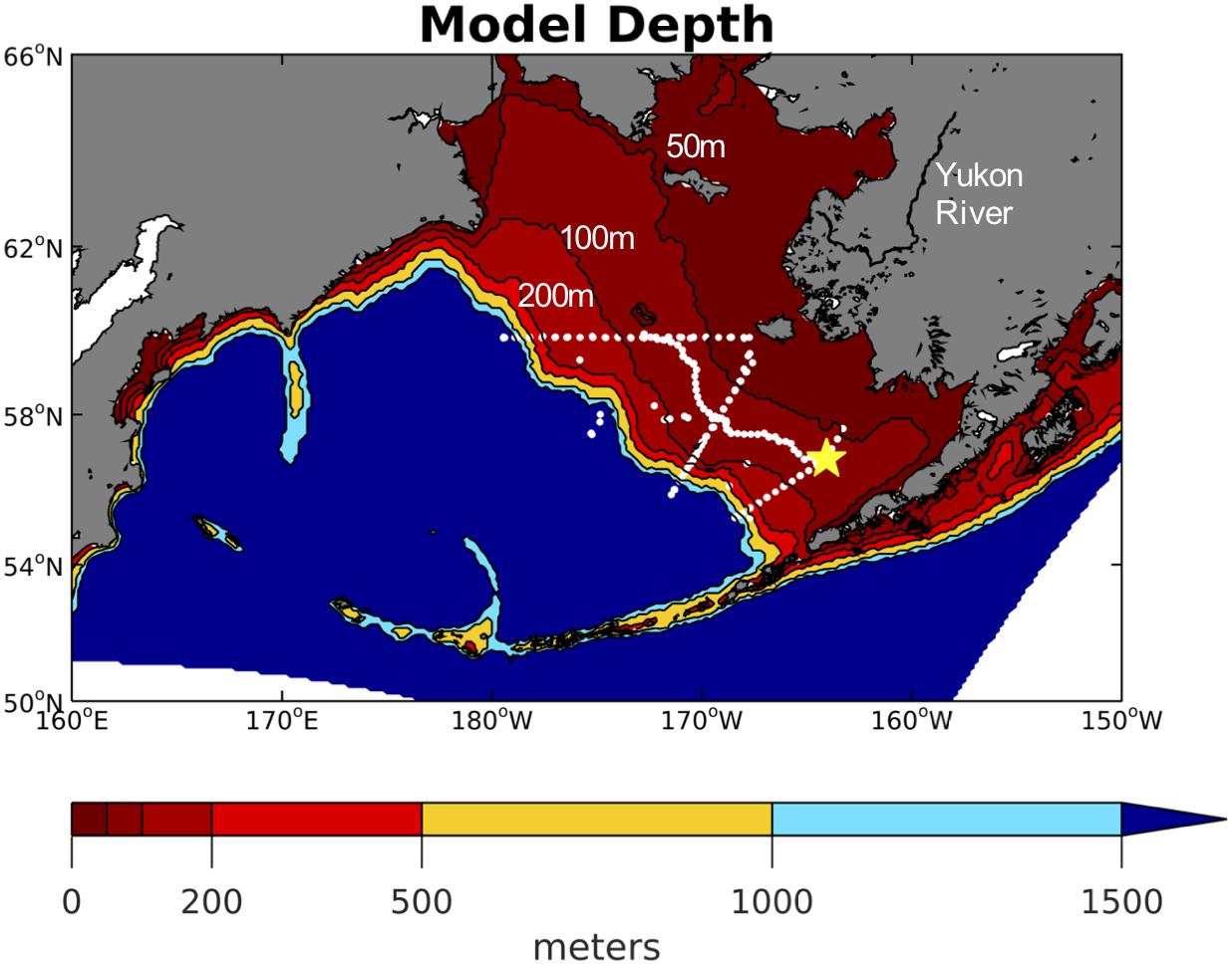
Figure 1. Model domain with contoured color shading for model depth. The contour lines for the 50, 100, and 200 m isobaths are also labeled as these represent the generalized boundaries for the inner, middle, and outer Bering Sea shelf domains. White dots signify station locations from the 2008–2010 BEST-BSIERP cruises and the yellow star signifies the locating of the M2 mooring.

Biogeochemical Model Description

We use the biological model developed as part of the BEST program by Gibson and Spitz (2011) (BEST-NPZD). This model contains 12 total pelagic state variables (Figure 2) – large and small phytoplankton, microzooplankton, small and large copepods, euphausiids, jellyfish, iron, nitrate, ammonium, and slow (1 m/day) and fast (10 m/day) sinking detritus. Coupled to this pelagic model is a 3-component ice-biology submodel which simulates ice algae, nitrate, and ammonium within the bottom 2 cm of the ice. Benthic processes are simulated in a 2-component benthic submodel consisting of benthic fauna and benthic detritus. Phytoplankton and detritus that sinks out of the bottom water layer enters the benthic detritus component. Of this flux, 20% is removed to simulate burial and off-shelf transport, based on observations at the M2 mooring (Figure 1; Gibson and Spitz, 2011). An additional 1% is removed due to de-nitrification, which is relatively low in the Bering Sea (Gibson and Spitz, 2011).

FIGURE 2

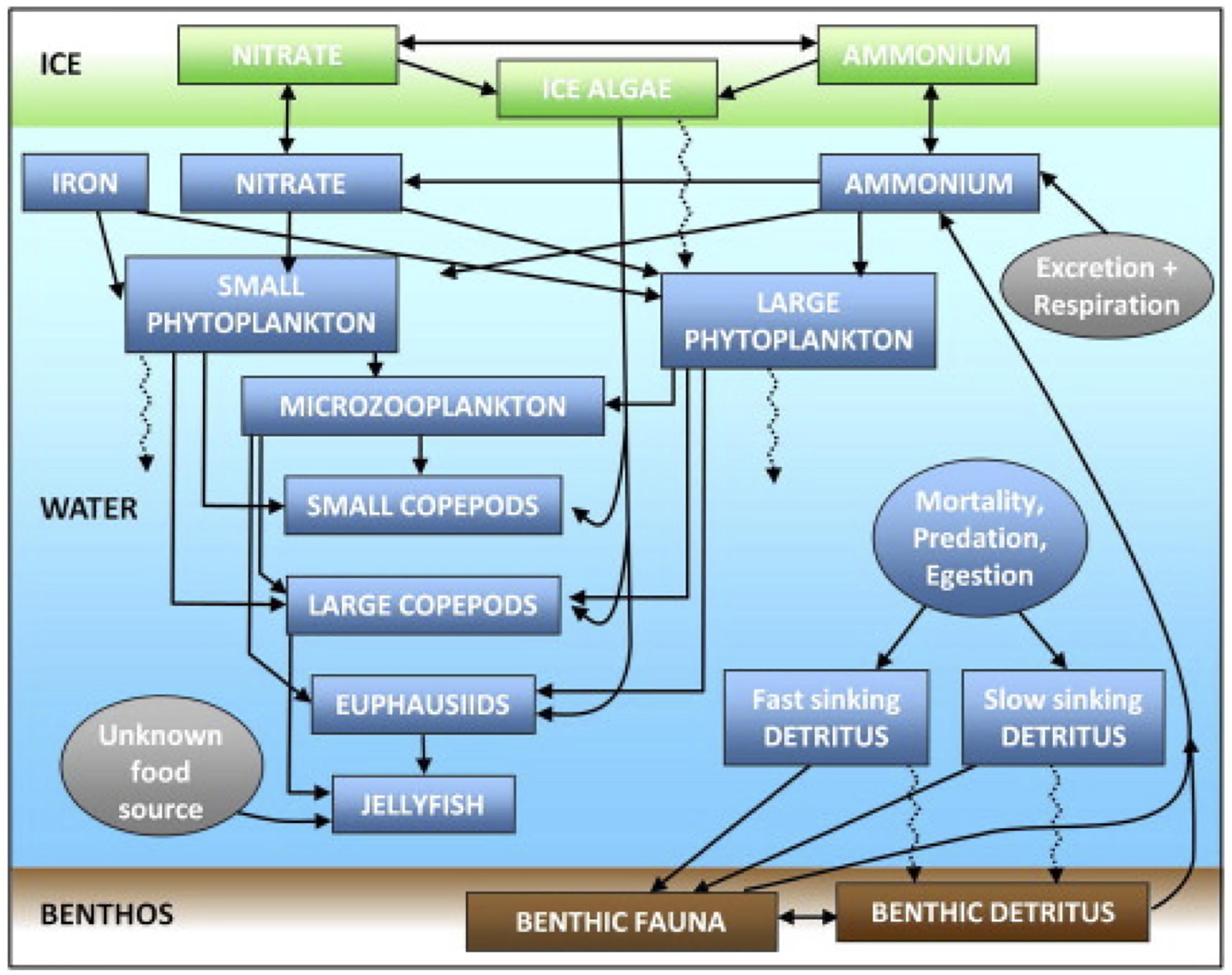
Figure 2. Schematic diagram of the model ecosystem structure, reprinted from Gibson and Spitz (2011) with permission from Elsevier.

We add dissolved inorganic carbon (DIC) and total alkalinity (TA) cycling to this existing biological model, following the framework of Fennel et al. (2008) for DIC and Siedlecki et al. (2017) for TA. The model is coded in units of carbon and is converted to nitrogen when necessary (e.g., for nitrate, ammonium, TA) following a constant C:N ratio of 106:16 (Sarmiento and Gruber, 2006). The time evolution of DIC is as follows:

\begin{array}{l} \frac{\partial D I C}{\partial t} = & r e m i n * D - P_{i} * μ_{i} (L i g h t, N) + R e s p (P_{i}) + \\ Z_{i} * G r a z_{i} (P_{i}) + a d v e c t i o n + d i f f u s i o n (1) \end{array}

\frac{\partial D I C}{\partial t} |_{b o t t o m} = \frac{1}{Δ z} (w_{D} \frac{d D}{d z} |_{z = b o t t o m}) (2)

\frac{\partial D I C}{\partial t} |_{s u r f a c e} = \frac{V_{C O 2}}{Δ z} * {[C O_{2}]}_{s o l} * ({[C O_{2}]}_{a i r} - [C O_{2}] |_{z = s u r f a c e}) (3)

V_{C O 2} = 0.31 u^{2} {(\frac{S c}{660})}^{- 0.5} (4)

where remin is the detrital (D) remineralization rate, P is the phytoplankton group, μ is the phytoplankton growth rate which is a function of light and nutrients (N), Resp is the respiration rate, Z is the zooplankton group, Graz is the zooplankton grazing rate, w_D is the sinking rate of 1 m/day for slow sinking detritus and 10 m/day for fast sinking detritus, [CO₂]_sol is the CO₂ solubility calculated from Weiss (1974), V_CO2 is the gas transfer velocity, u is the wind speed, Δz is the vertical thickness of the model grid cell, z = bottom is the bottom water model grid cell, and Sc is the Schmidt number from Wanninkhof (1992). The atmospheric CO₂ concentration ([CO₂]_air) is set to a spatially mean value at monthly time resolution from 2002 to 2012, calculated for the Bering Sea from the NOAA Earth System Research Laboratory’s CarbonTracker 2016 product (CT2016; Peters et al., 2007). Atmospheric CO₂ increases from 370 μatm to 393 μatm over the 10-year model hindcast.

Alkalinity cycling follows many of the same processes as DIC, except with the addition of nitrification and the lack of air-sea exchange:

\begin{array}{l} \frac{\partial T A}{\partial t} = & P_{i} * μ_{i} (L i g h t, N O_{3}) - P_{i} * μ_{i} (L i g h t, N H_{4}) + \\ r e m i n * D + r e s p (P_{i}) + Z_{i} * G r a z_{i} (P_{i}) - 2 * N i t r i f + \\ a d v e c t i o n + d i f f u s i o n (5) \end{array}

\frac{\partial T A}{\partial t} |_{b o t t o m} = \frac{1}{Δ z} (w_{D} \frac{d D}{d Z} |_{z = b o t t o m}) (6)

where Nitrif is nitrification. Phytoplankton uptake of nitrate (NO₃^-) increases TA while the uptake of ammonium (NH₄⁺) decreases TA (Brewer and Goldman, 1976; Goldman and Brewer, 1980; Zeebe and Wolf-Gladrow, 2001; Siedlecki et al., 2017). Nitrification decreases TA due to the production of H⁺ from the conversion of ammonium to nitrate (Brewer and Goldman, 1976).

DIC and TA are not explicitly simulated within the ice sub-model, however, surface layer DIC and TA concentrations are directly modified by ice algae growth, in order to ensure mass conservation. For example, growth of ice algae decreases surface water DIC, which is then transferred back to the water column following ice algae senescence, grazing, or sinking. A caveat of this simplified approach is that it ignores any additional dynamics between sea ice and TA/DIC, which may have significant local effects in Arctic environments. For example, the formation of ikaite crystals in sea ice can have a greater impact on surface water pCO₂ concentrations than ice algae production (Rysgaard et al., 2012; Moreau et al., 2014). To our knowledge, this effect has not been quantified in a 3D biogeochemical model, so we leave this to future work. The presence of sea ice also acts to inhibit the magnitude of the air-sea CO₂ flux according to the percentage of the grid cell covered by ice. For example, a grid cell that is 40% covered with sea ice will have the flux magnitude reduced by 40%.

Boundary Conditions

Oceanic horizontal open boundary conditions are interpolated from the CFSR/CFSv2 global model reanalysis/analysis (for all physical state variables) and climatological estimates (for BEST-NPZ state variables). Values for TA and DIC are derived from empirical relationships with salinity, calculated from shipboard data collected as part of the BEST-BSIERP program from 2008 to 2010. Sampling typically occurred between April and July, with an additional late September to early October cruise in 2009. The values are calculated using the following robust linear regressions:

S < 32.6 D I C = 58.5 * S + 191.2 (7)

S \geq 32.6 D I C = 140.4 * S - 2478.7 (8)

S < 33.6 T A = 49.6 * S + 600.6 (9)

S \geq 33.6 T A = 141.8 * S - 2494.4 (10)

This method was previously employed by Siedlecki et al. (2017) for the Gulf of Alaska, which yielded similar fits, suggesting that the fits are robust throughout the region. All of the fits display strong R² values (0.75–0.95), except for the DIC fit at salinity values less than 32.6 psu (R² = 0.21). This fit can be moderately improved by increasing the value of the salinity cutoff between the two fits, however, this leads to a discontinuity where the two regressions intersect. This discontinuity can generate substantial differences in DIC values between two very similar salinities and is therefore less suitable for our purpose of simulating the model boundary conditions.

Freshwater terrestrial runoff reduces salinity in nearshore gridpoints, with monthly climatological magnitude calculated from Dai et al. (2009). The freshwater runoff also has a seasonally varying concentration of DIC and TA following data collected from the mouth of the Yukon River (Table 1). The Yukon River supplies a substantial portion of the total freshwater runoff to the Bering Sea, and is therefore a reasonable representation of total runoff flux of DIC and TA to the Bering Sea. Model water column iron, nitrate, and ammonium are relaxed to climatological values on a 1-year timescale in order to reduce any long-term drift issues that may develop on decadal model timeframes (Hermann et al., 2013). Climatology values are based on observational data collected in the Bering Sea (e.g., BEST-BSIERP), with some additional tuning based on model ecosystem development and multidecadal hindcast analysis (Gibson and Spitz, 2011; Hermann et al., 2013). This climatological relaxation was found to have no discernable impact on 4-year timeframes, but is essentially for multidecadal runs (Hermann et al., 2013). Model surface salinity values are relaxed to monthly values from the Polar Science Center Hydrographic Climatology (PHC; Steele et al., 2001), using the same 1-year relaxation timescales as was used for the nutrients. Model initial conditions for all prognostic variables except TA and DIC are interpolated from a long-term spinup of the Bering10K model, started in 1970 and fully described in Hermann et al. (2013). Initial conditions for TA and DIC are calculated from the salinity regressions.

TABLE 1

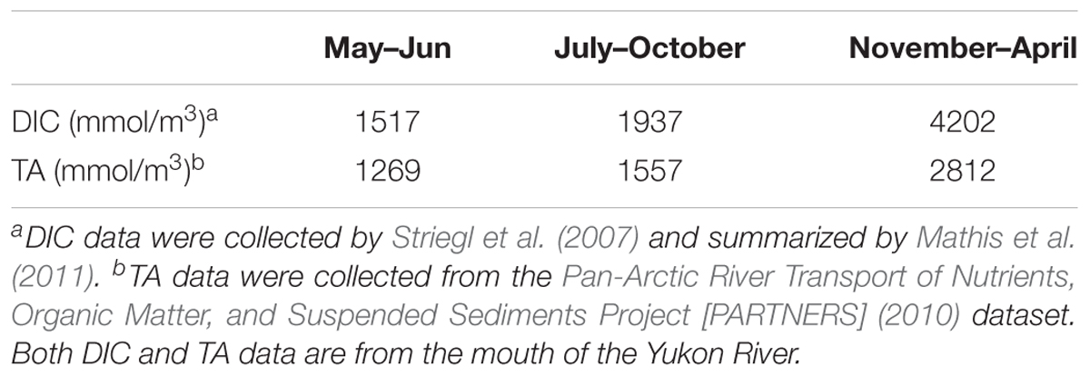
Table 1. Seasonal concentrations of DIC and TA in freshwater runoff.

Model Skill Assessment

We use observational shipboard data collected during the 2008–2010 BEST-BSIERP cruises for model validation. These data were collected during the spring (April/May) and summer (June/July) seasons, with an additional fall (September/October) sampling in 2009. The sampling covered three cross-shelf transects and one line along the 70 m isobath (Figure 1). Model output is compared to co-located discrete measurements of temperature, salinity, nitrate, DIC, and TA. Values of pCO₂ and Ω_Arag were calculated from TA and DIC by Cross et al. (2012, 2013) using CO2SYS version 1.05 (Lewis and Wallace, 1998). Model comparisons to observed data are summarized with target diagrams (Jolliff et al., 2009). Target diagrams allow for easy visualization of a model’s bias and variance compared to the observed data. Location on the y-axis indicates either a positive (Y > 0) or negative (Y < 0) model bias, while location on the x-axis (calculated as the normalized unbiased RMSD between model and data, multiplied by the sign of modeled minus observed standard deviation) indicates whether the model has a larger (X > 0) or smaller (X < 0) standard deviation compared to the observed data. The radial distance from the origin is also related to the modeling efficiency metric (MEF; Stow et al., 2009). Model fields that lie within the circle have a MEF value of less than 1, indicating better than average model performance as compared to using the mean of the observations. A “perfect” fit would result in all points at X = 0, Y = 0.

Model Hindcast Setup

The model hindcast was run from 2002 to 2012. The year 2002 serves as the model spin-up year for the DIC and TA tracers, therefore we only display results from 2003 to 2012. To ensure sufficient model spin-up, we also tested using two consecutive years of 2002 forcing, but found no substantial subsequent model differences compared to the single year of 2002 forcing. Upon model completion, the model output is re-gridded from the curvilinear, sigma-coordinate grid to a regular latitude-longitude-depth grid to facilitate plotting and comparison to observational data.

Results

Model Performance

The Bering10K model with the BEST-NPZD ecosystem model has been previously validated and utilized in a variety of studies exploring biophysical variability in the Bering Sea in both hindcast and decadal projection simulations (Gibson and Spitz, 2011; Hermann et al., 2013, 2016; Ortiz et al., 2016). The model version presented in this manuscript incorporates updated algorithms for the vertical absorption of shortwave radiation in the water column and sea ice growth described in Hermann et al. (2016). These updated algorithms significantly improved model-data comparisons of water temperature and sea ice coverage. The model does contain a few previously described biases, including a late sea ice retreat and colder water temperatures in the northern regions (Hermann et al., 2016). This late sea ice retreat also delays the timing of the spring bloom and tends to generate somewhat lower total phytoplankton biomass in spring and greater biomass in fall (Ortiz et al., 2016). The model version used in the present study also includes recent corrections to the ice thermodynamics terms, which reduce but do not completely eliminate these biases (K. Kearney, personal communication).

Most model fields compare well with the observations and fall within the MEF < 1 circle, suggesting that the model is skillful at reproducing the observed system (Figure 3). The lack of any significant mean biases suggest that the model is especially useful for simulating mean-state conditions, particularly near the surface. Only surface TA and NO₃^- values fall outside of the circle, underestimating and overestimating the observed variability respectively. This bias in variability for surface NO₃^- suggests that the model may be producing more variability in nutrient transport or primary productivity. The biases described above by Ortiz et al. (2016) support the latter mechanism. However, if primary productivity variability is overestimated, we may also expect to see an overestimate in DIC variability. On the contrary, DIC variability is underestimated. Thus, either this mechanism is not present, is not of sufficient magnitude to produce a similar bias in DIC, or is compensated by additional factors governing DIC variability (e.g., TA, air-sea CO₂ flux, solubility).

FIGURE 3

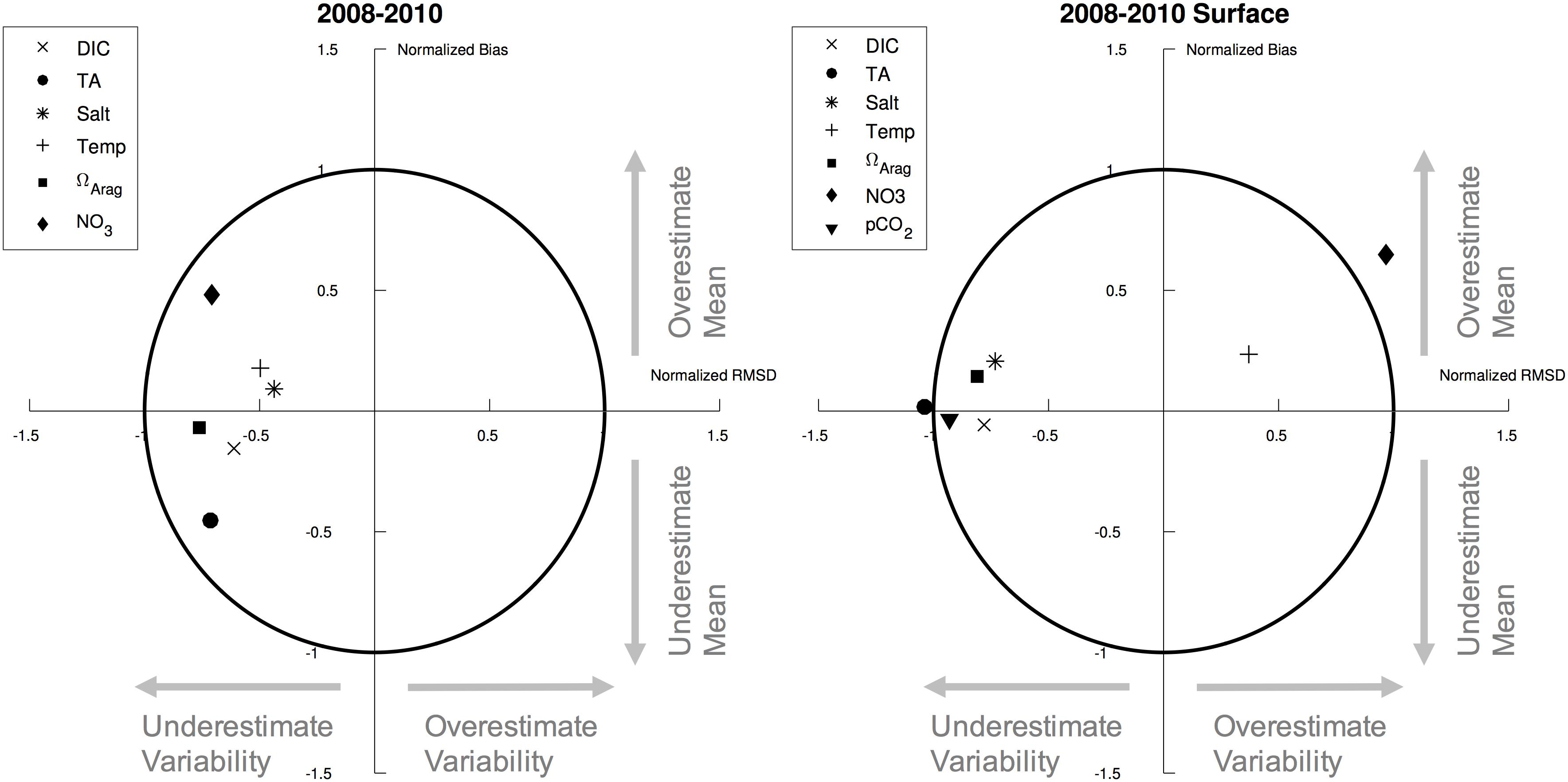
Figure 3. Target diagrams for model variables compared to observed variables from the 2008–2010 BEST-BSIERP cruises for (left) the full water column and (right) surface layer. X-axis is the normalized unbiased RMSD between model and data, multiplied by the sign of the difference between modeled standard deviation and observed standard deviation. Y-axis is the normalized mean bias between model and data. The symbol locations thus illustrate whether the model contains a positive (Y > 0) or negative (Y < 0) bias, whether the model standard deviation is larger (X > 0) or smaller (X < 0) compared to the observations, and the normalized unbiased RMSD between model and data (absolute value of X).

Seasonal and Spatial Patterns

The direction of the air-sea flux of CO₂ is determined by the gradient between the pCO₂ of the surface ocean (pCO₂^ocn) of the atmosphere (pCO₂^atm). Here we define this gradient as the ΔpCO₂ (pCO₂^ocn – pCO₂^atm), where a negative value indicates a flux direction from the atmosphere into the ocean. Thus, regions of negative ΔpCO₂ are associated with regions of net ocean carbon uptake.

Values of ΔpCO₂ are generally neutral on the Bering Sea shelf throughout most of the winter and spring, but become largely negative in summer and fall (Figure 4). In particular, June–October ΔpCO₂ values are strongly undersaturated with respect to the atmosphere, typically ranging from -100 to -200 μatm. However, much of the coastal ocean near western Alaska and Nunivak Island contains positive ΔpCO₂ values, particularly near the Yukon River delta. In the deep-water basin off of the Bering Sea shelf, ΔpCO₂ remains slightly positive or neutral for nearly the entire year. CO₂ flux values display a similar seasonal pattern but with differences in relative magnitude due to the influence of wind speed and sea ice (Figure 5). For example, sea ice inhibits air-sea exchange on the inner and middle coastal shelf during winter and spring months, leading to relatively low CO₂ flux values. Conversely, frequent storms and strong wind speeds produce substantial positive CO₂ flux values of 20–30 mmolC/m²/day in the deep Bering Sea basin despite relatively low ΔpCO₂ values (∼ 25–50 μatm).

FIGURE 4

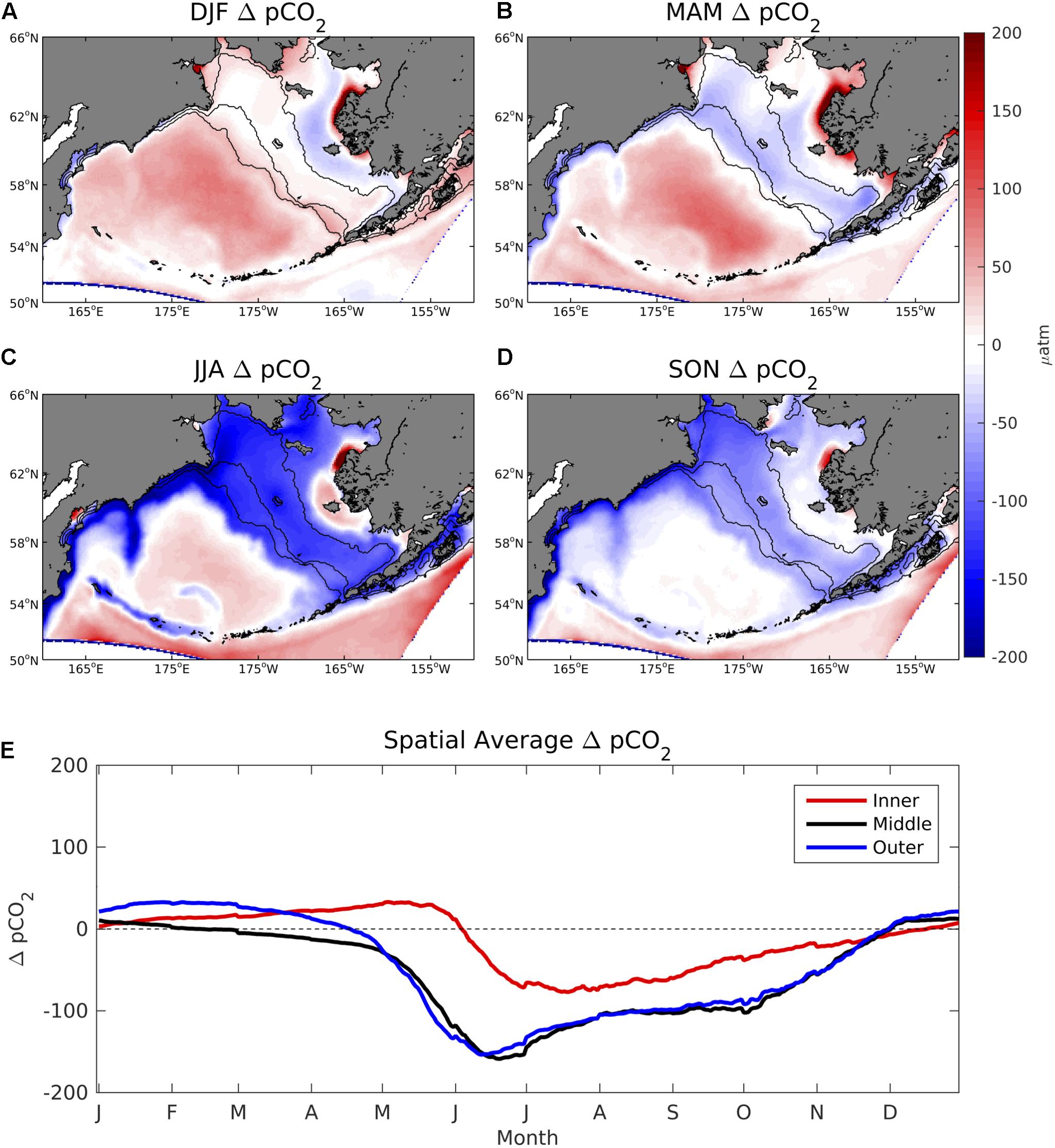
Figure 4. (A–D) Seasonal plots of model ΔpCO₂ averaged over the 2003–2012 timeframe and (E) time series of area-weighted spatial mean ΔpCO₂ for the three shelf domains, denoted by the 50, 100, and 200 m isobath lines shown in Figure 1.

FIGURE 5

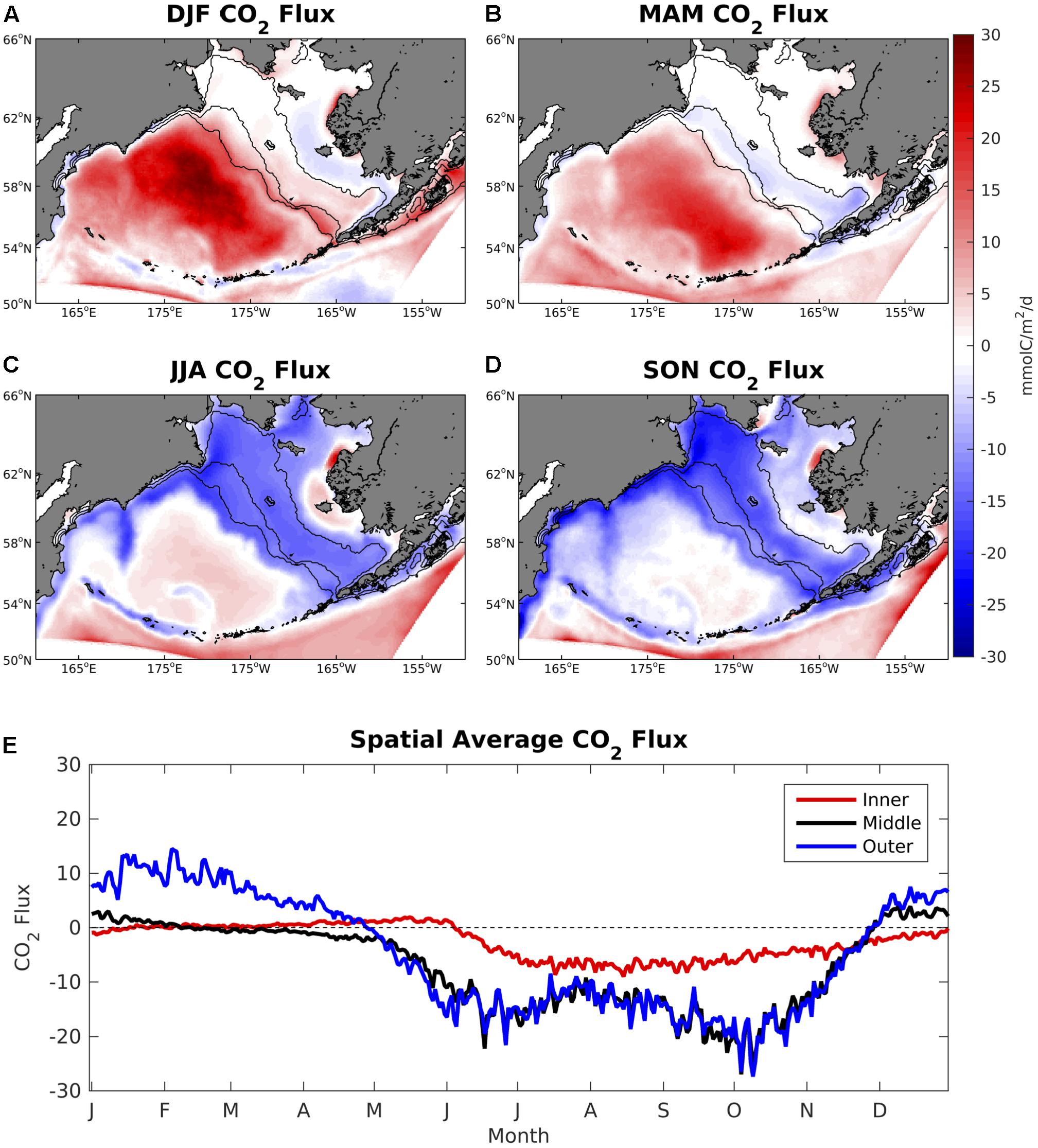
Figure 5. (A–D) Seasonal plots of model air-sea CO₂ flux averaged over the 2003–2012 timeframe and (E) time series of area-weighted spatial mean CO₂ flux for the three shelf domains. A positive value signifies a flux of carbon from the ocean to the atmosphere.

Values of surface Ω_Arag are relatively low throughout winter and spring, with values in coastal regions along the western Alaskan shoreline consistently below 1 (Figure 6). Ω_Arag values increase to 2–3 during summer and fall for most of the Bering Sea shelf, except for coastal regions near Nunivak Island and the Yukon River delta where Ω_Arag remains less than 2 and less than 1 in a few isolated locations. Bottom water Ω_Arag values are lower compared to the surface and display a more subdued seasonal cycle compared to surface Ω_Arag (Figure 7). Coastal waters along the western Alaskan shoreline are persistently undersaturated in aragonite through winter and spring similar to surface waters, however, coastal regions near Siberia are also undersaturated for large portions of the year. Regions along the middle and outer Bering Sea shelf also display an inverse seasonal cycle compared to surface Ω_Arag. That is, bottom water Ω_Arag values decrease during the winter-summer transition, as opposed to surface Ω_Arag values which increase.

FIGURE 6

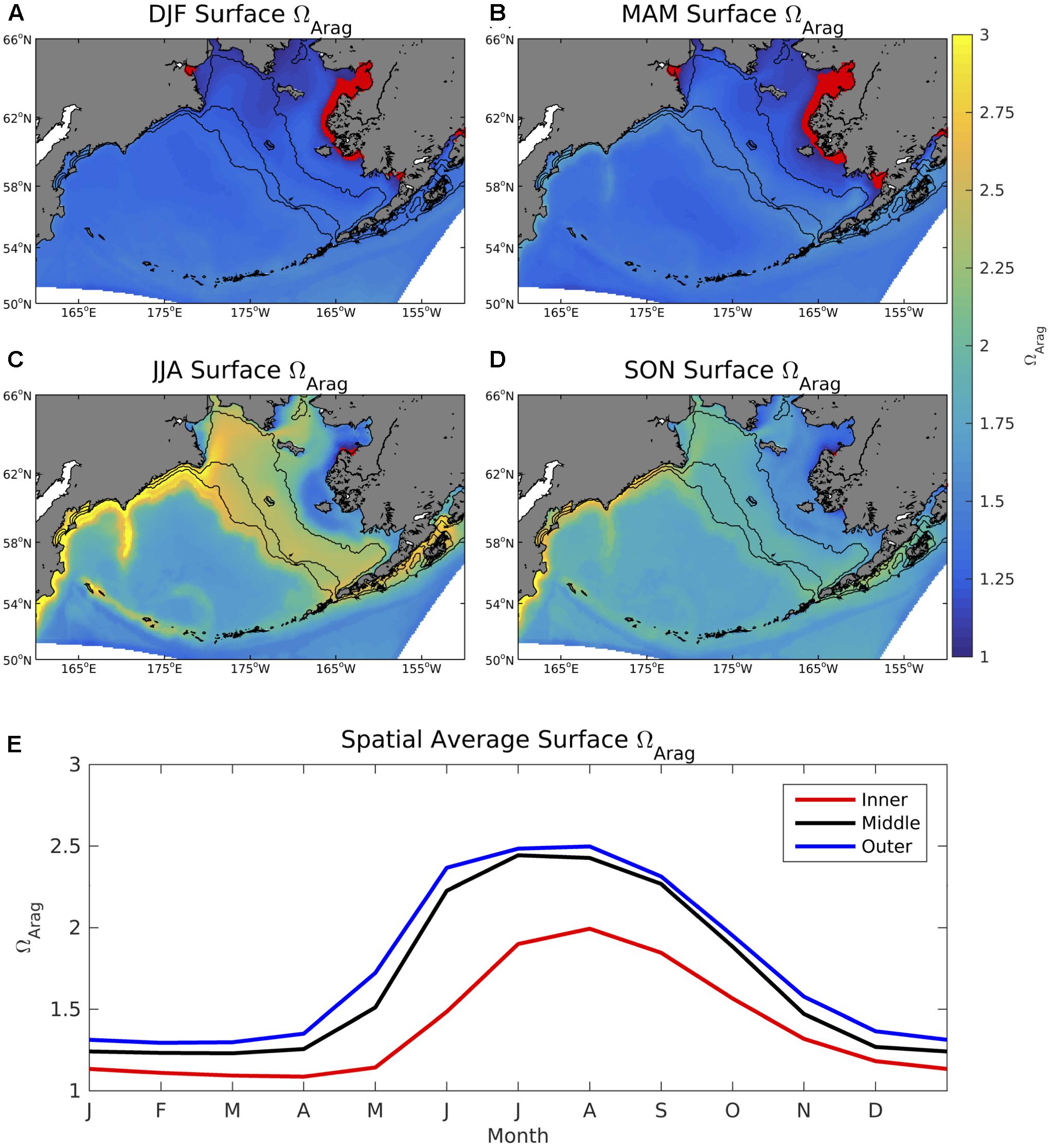
Figure 6. (A–D) Seasonal plots of model surface Ω_Arag averaged over the 2003–2012 timeframe and (E) time series of area-weighted spatial mean Ω_Arag for the three shelf domains The red dots signify locations where Ω_Arag < 1.

FIGURE 7

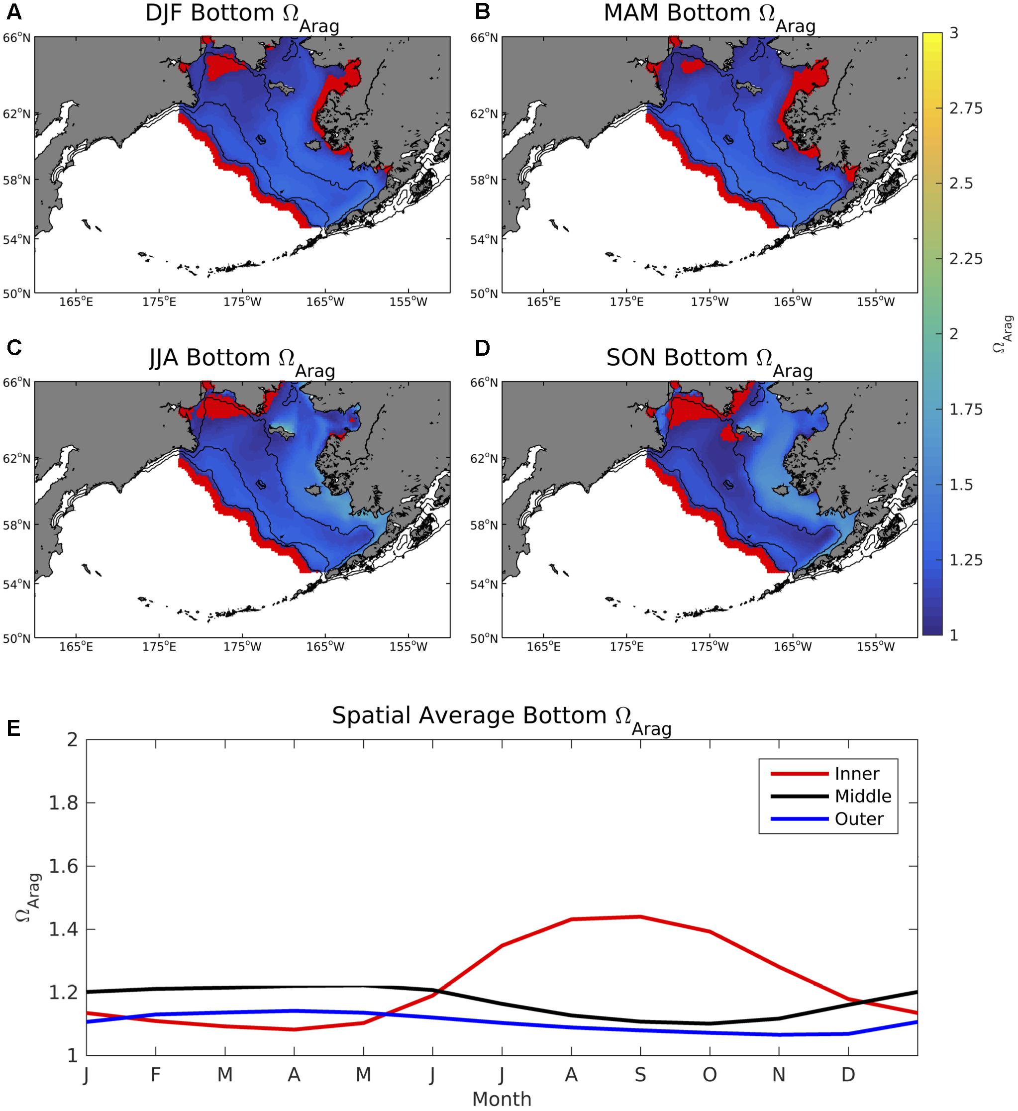
Figure 7. (A–D) Seasonal plots of model bottom water Ω_Arag averaged over the 2003–2012 timeframe and (E) time series of area-weighted spatial mean bottom Ω_Arag for the three shelf domains. The red dots signify locations where Ω_Arag < 1. Regions deeper than the Bering Sea coastal shelf break (>1500 m) are whited out.

The spatial differences between the inner and outer Bering Sea shelf also manifest on annual timescales, with important implications to the underlying carbon chemistry (Figure 8). Salinity, DIC, and TA are all substantially lower along the inner shelf compared to the rest of the model domain, and particularly within Norton Sound, indicative of outflow from the neighboring Yukon River delta. Plotting the TA/DIC ratio (Figure 8E) illustrates the relative buffering capacity of the water, with lower values indicating a reduced buffering capacity. Values along the inner shelf are relatively lower compared to the outer shelf, indicating this reduced buffering capacity. The spatial pattern of the TA/DIC ratio correlates very strongly with the spatial pattern in Ω_Arag (r = 0.996, Figure 8F), illustrating the utility of this ratio in identifying regions of corrosive water conditions. Relatively low phytoplankton productivity on the inner shelf and high productivity on the outer shelf (Figure 8B) further contributes to the spatial pattern of this ratio through changes in DIC.

FIGURE 8

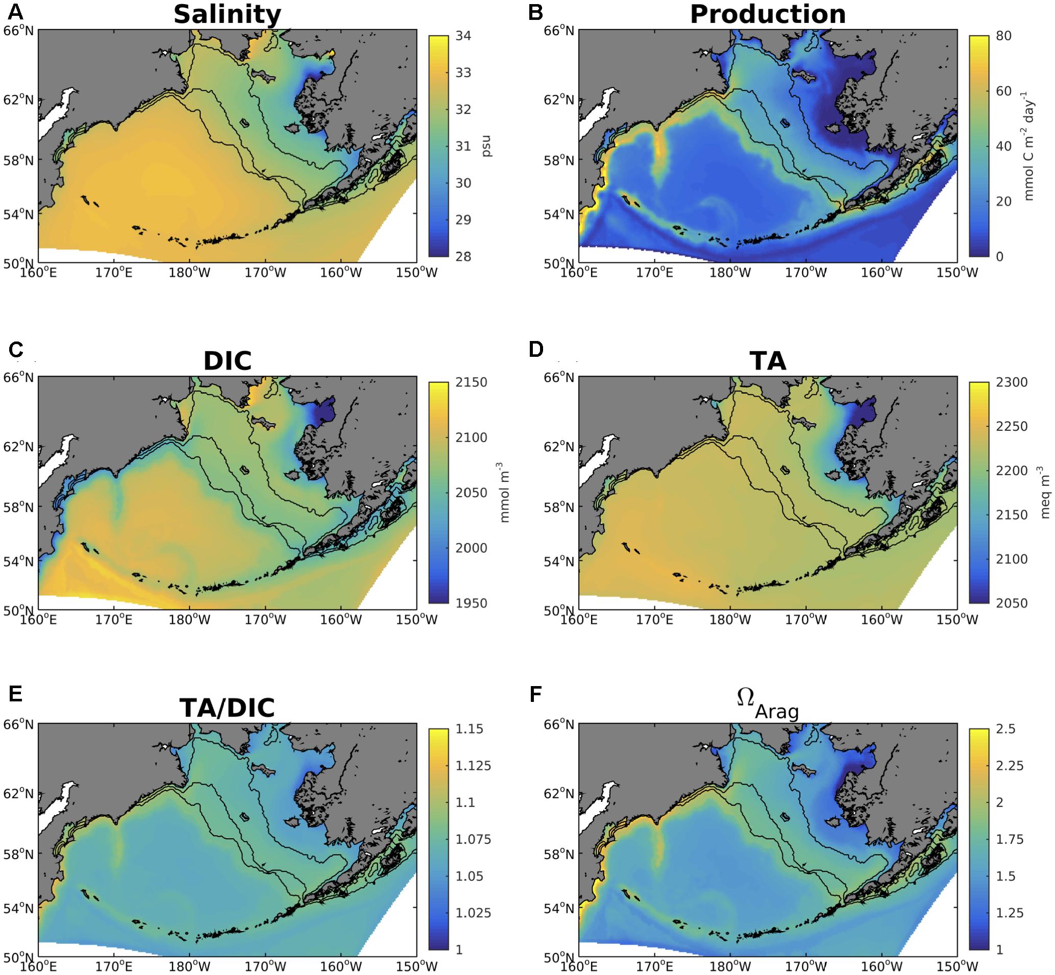
Figure 8. Annual average plots of model (A) surface salinity, (B) primary production integrated over the top 200 m of the water column, (C) surface DIC, (D) surface TA, (E) surface TA/DIC ratio, and (F) surface Ω_Arag. All variables are averaged over the 2003–2012 timeframe.

Warm and Cold Regimes

The model hindcast timeframe covers two distinct observed temperature regimes: a period of warm, relatively low sea ice extent years (2003–2005) and a period of cold, relatively high sea ice extent years (2010–2012). Surface water temperatures during the cold regime are generally 1–2°C colder throughout most of the shelf region, and up to 4°C colder along the southeastern middle and outer shelf domains (Figures 9A–C). Similarly, sea ice extent is 20–40% greater during the cold regime (Figures 9D–F). Primary production increases for the outer shelf and the northwestern shelf, but remains largely unchanged or slightly decreases through most of the inner shelf and for Bristol Bay (Figures 9G–I). Surface salinity slightly decreases for the outer and middle shelf, but slightly increases for the inner shelf (Figures 9J–L). During the transition from a warm to a cold period, surface Ω_Arag decreases by ∼ 0.2 units throughout most of the Bering Sea shelf, with locations south of Nunivak Island and in Bristol Bay decreasing by up to 0.3 units (Figures 10A–C). Surface Ω_Arag also decreases in the Bering Sea Basin, though to a lesser extent (∼0.1 units) compared to the shelf. Surface DIC increases by 20 mmol/m³ for most of the shelf, with a smaller increase of 5–10 mmol/m³ along the shelf break region (Figures 10D–F). However, the area around Nunivak Island remains largely unchanged. Surface TA remains relatively unchanged for the middle and outer coastal shelf, but decreases by ∼20 meq/m³ for large portions of the inner shelf near Nunivak Island (Figures 10G–I). The change in air-sea CO₂ flux is more spatially heterogeneous than the change in Ω_Arag and DIC (Figures 10J–L). Following a similar pattern to primary production (Figures 9G–I), CO₂ flux becomes more negative (i.e., increased ocean carbon uptake) over the outer and northwestern shelf regions, but more positive over the inner shelf. In particular, the outer shelf region near the Aleutian Island chain transitions from a neutral or weak carbon source to a significant carbon sink. Carbon efflux from the deep Bering Sea basin also decreases, though the region remains a significant carbon source on annual timeframes.

FIGURE 9

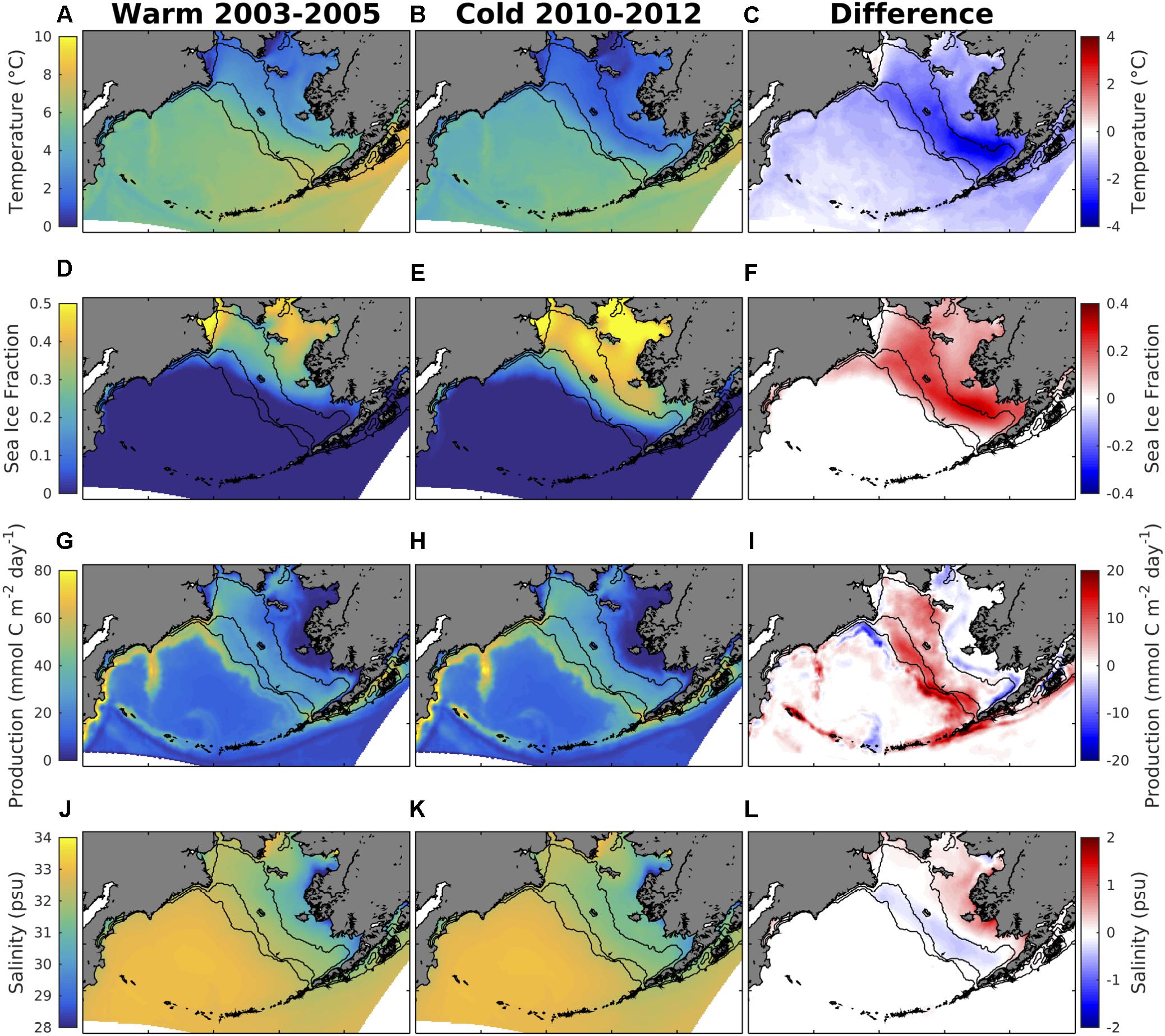
Figure 9. (left) Model annual mean variables averaged over the warm and (middle) cold temperature regimes, and (right) the difference generated by the transition from warm to cold conditions. (A–C) Surface temperature, (D–F) fraction of grid cell covered by sea ice, (G–I) production integrated over the top 200 m of the water column, and (J–L) surface salinity.

FIGURE 10

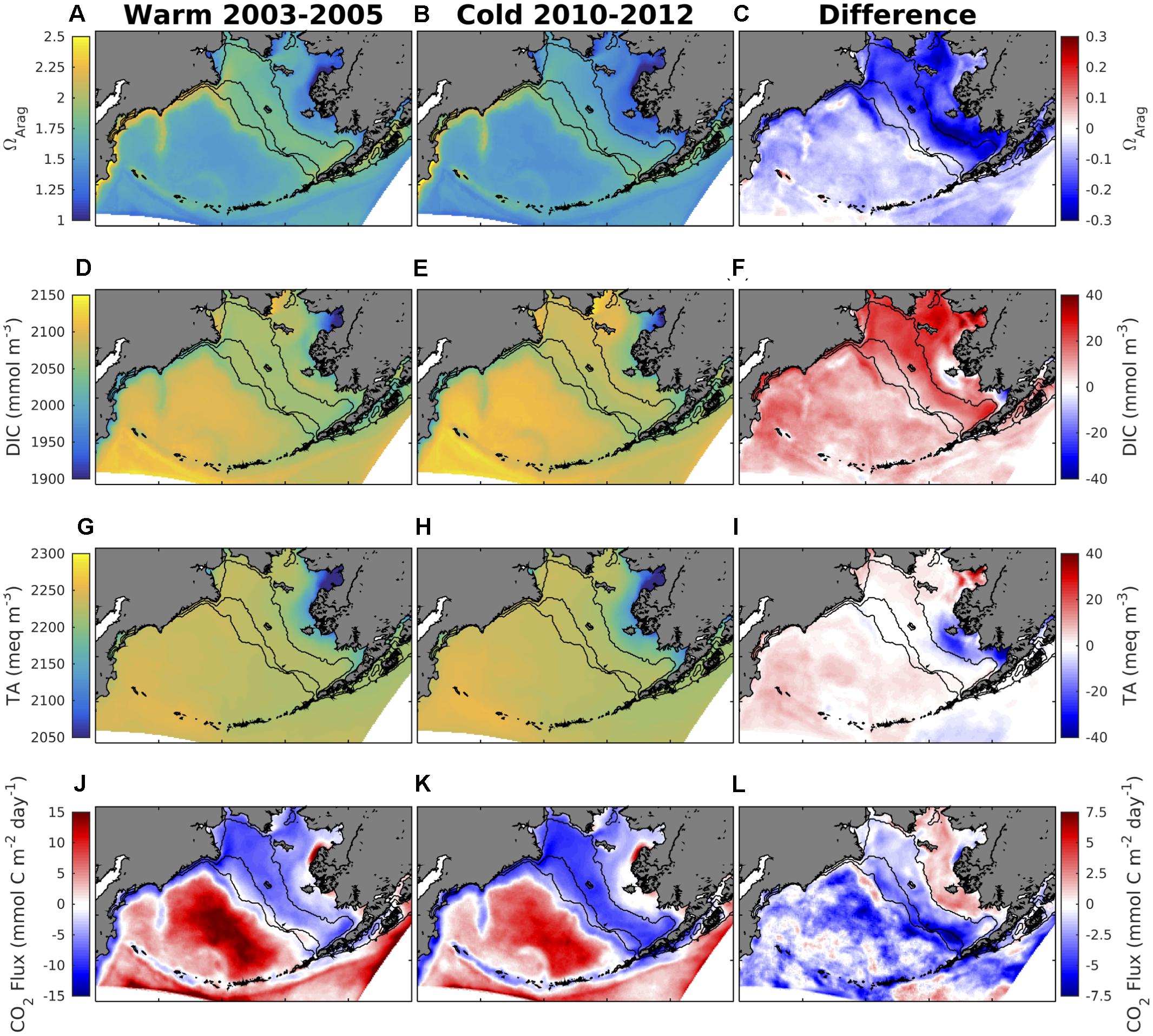
Figure 10. (left) Model annual mean variables averaged over the warm and (middle) cold temperature regimes, and (right) the difference generated by the transition from warm to cold conditions. (A–C) Surface Ω_Arag, (D–F) surface DIC, (G–I) surface TA, and (J–L) air-sea CO₂ flux (where a positive value indicates a flux out of the ocean).

Decadal Trends

Statistically significant trends (p-value < 0.05) of decreasing Ω_Arag are evident throughout most of the Bering Sea shelf, with magnitudes ranging from 0.025 – 0.04 units/year (Figure 11). These regions also correspond to significant positive trends in DIC of 2.5 – 4.0 mmol/m³/year. Localized regions of negative trends in TA of -2.5 to -5.0 mmol/m³/year are also present in the southeastern inner shelf. Trends in pCO₂ and ΔpCO₂ are largely positive along the inner and northwestern middle Bering Sea shelf, but large portions of the outer and southeastern middle shelf display a negative trend, particularly for ΔpCO₂. These areas of significant negative ΔpCO₂ trends correspond to regions of significant negative trends in CO₂ flux, indicating an increase in ocean carbon uptake.

FIGURE 11

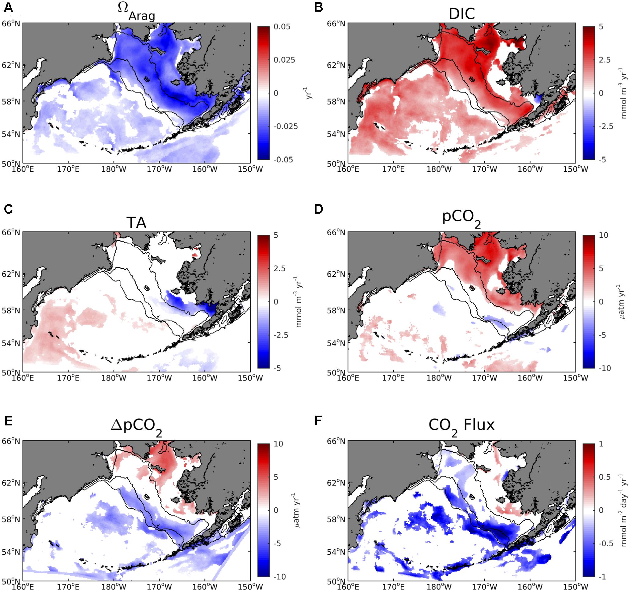
Figure 11. Linear trends in annual average surface model (A) Ω_Arag, (B) DIC, (C) TA, (D) pCO₂, (E) ΔpCO₂, and (F) air-sea CO₂ flux. Linear trends are calculated using the 2003–2012 timeframe. Only trend values that are significant at the 95% confidence level are displayed.

The negative trends in CO₂ flux drive positive trends in surface pCO₂ and DIC, along with a substantial increase in the total carbon uptake of the entire Bering Sea shelf (Figure 12). Surface ocean pCO₂ largely follows the estimated, expected increase in ocean pCO₂ based on the air-sea pCO₂ disequilibrium calculated in 2002 and the increase in atmospheric CO₂ over the model hindcast timeframe (Figure 12A). We then recalculate DIC using CO2SYS and the ocean pCO₂ values calculated in Figure 12A (dashed line), along with model TA, salinity, and temperature (Figure 12B). This allows for comparison between the model increase in surface DIC and the expected increase in DIC, calculated from the increase in ocean pCO₂ associated with the increase in atmospheric CO₂. The goal is to understand the extent to which the change in model pCO₂ and DIC is driven by the increase in atmospheric CO₂. Figure 12B illustrates that the two values track closely, similar to Figure 12A. Shelf annual total carbon uptake increases from 15.9 TgC/year in 2003 to 26.3 TgC/year in 2012, and total benthic carbon increases slightly from 2.61 TgC in 2003 to 2.78 TgC in 2012 (Figures 12D,E). Surface Ω_Arag decreases from 1.7 to 1.5, while bottom Ω_Arag decreases from 1.2 to 1.1. Thus, the decrease at the surface is approximately twice as great as the decrease at the bottom.

FIGURE 12

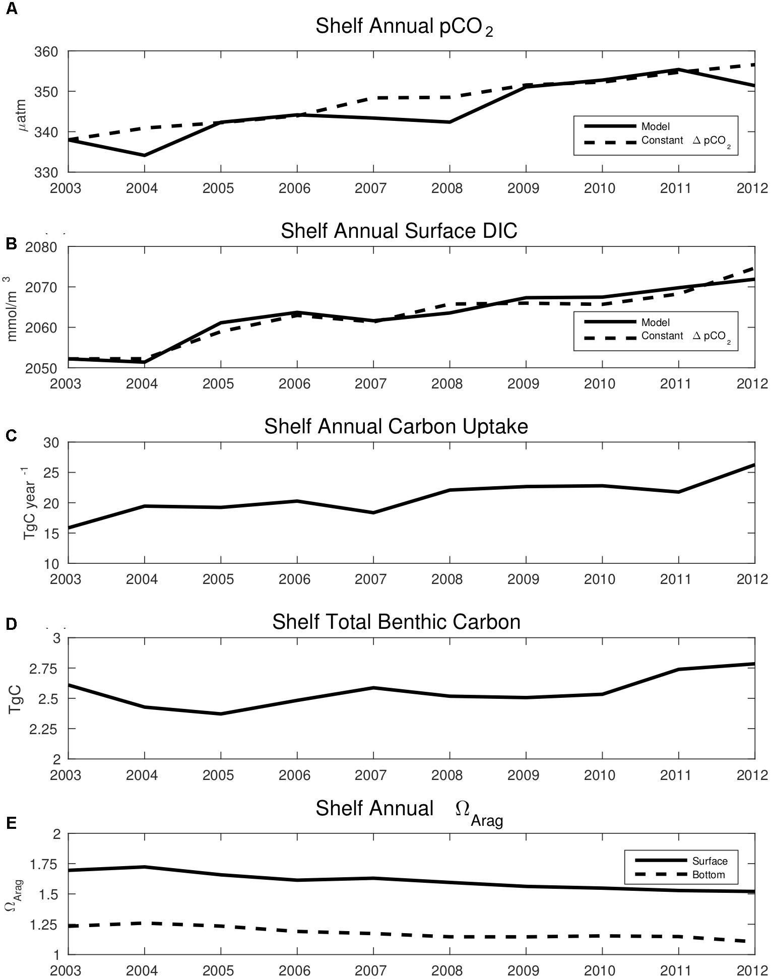
Figure 12. Time series plots of annual average model (A) surface ocean pCO₂ and (B) surface DIC. The dashed line in (A) represents the expected increase in surface ocean pCO₂ based on the model air-sea pCO₂ disequilibrium in 2003, combined with the yearly increase in atmospheric CO₂. The dashed line in (B) represents the excepted increase in surface ocean DIC, calculated from the expected surface pCO₂ values shown in the dashed line of (A), and the model values of total alkalinity, salinity, and temperature. (C) Total ocean carbon uptake and (D) total benthic carbon over the entire Bering Sea shelf. (E) Annual average values of surface Ω_Arag (solid line) and bottom water Ω_Arag (dashed line).

Discussion

The model simulates significant spatial variability in carbonate chemistry on the Bering Sea shelf, resulting from local biogeochemical processes. The inner shelf region contains low values of Ω_Arag, with some areas near the Yukon Delta and Norton Sound experiencing nearly year-round Ω_Arag < 1 conditions. These corrosive water conditions result from river inputs of terrestrial carbon from the Yukon River combined with low coastal productivity, which both drive a reduced TA/DIC ratio. Previous studies using shipboard data have also noted relatively low productivity and Ω_Arag waters along the inner shelf (Mathis et al., 2011; Cross et al., 2014), though the corrosive conditions in Norton Sound are difficult to verify due to a lack of data. Norton Sound contains a relatively small red king crab fishery, but the life cycle of these crab is largely unknown (Norton Sound Economic Development Corporation [NSEDC], 2016). The sound may therefore be a natural analog to future OA conditions and an ideal location for experimental testing on the impacts of OA on red king crab growth, survival, and adaptability. However, observational data are first needed to verify these corrosive water conditions.

In contrast to the inner shelf, the middle and outer shelf regions have greater values of Ω_Arag, particularly during the summer and fall, due to substantial productivity and minimal influence of freshwater runoff. While this productivity boosts Ω_Arag in surface waters, carbon remineralization at depth generates bottom water Ω_Arag values close to 1. This result is supported by observational evidence (Mathis et al., 2014) and is noteworthy because the region is home to substantial tanner and red king crab fisheries, which are negatively impacted at Ω_Arag values less than 1 (Long et al., 2013; Mathis et al., 2015a; Long et al., 2016). Furthermore, while summer and fall surface Ω_Arag is highly saturated due to productivity, winter and early spring values are much lower at 1.0–1.5. Thus, while productivity may buffer Ω_Arag against OA during the summer and fall, biological organisms are still highly vulnerable to winter and early spring conditions as Ω_Arag values are already near 1.

Modeled total annual carbon uptake for the Bering Sea shelf is 15–25 TgC/year, which is within the 2–67 TgC/year range of previous estimates, but is significantly greater than the most recent estimate of 6.8 TgC/year (Cross et al., 2014). This difference between the latter estimate and the model results from substantially greater modeled carbon uptake in fall. Cross et al. (2014) report average CO₂ flux values of -5.0 and -0.48 mmolC/m²/day in September and October respectively, whereas model average flux values are between -10 and -15 mmolC/m²/day for these months. These higher magnitude model flux values are caused by a fall phytoplankton bloom, generated by vertical mixing of nutrients under still-optimal light and temperature conditions (Figure 13). Similar fall blooms are observed on the eastern Bering Sea shelf (Sigler et al., 2014) and reproduced in other biogeochemical models (Cheng et al., 2016), but their prevalence has received less attention compared to the spring bloom. This fall biological drawdown is not apparent to the same extent in the Cross et al. (2014) analysis, though they still calculate a pCO₂ drawdown of 50–100 μatm in September and October due to biological productivity. The data are also sparser in September and October compared to the spring and summer months, primarily consisting of a north-south transect line from the Aleutian Islands to the Bering Strait. In this transect, relatively larger ΔpCO₂ of ∼150 μatm are located on the outer and middle shelf region south of Nunivak Island, similar to the region of enhanced model primary productivity. It is possible that the finer spatial and temporal resolution of the model is capturing this fall productivity signal that is largely absent in the observed pCO₂ data, though the model is also likely biased considering the stronger magnitude fall bloom (Ortiz et al., 2016).

FIGURE 13

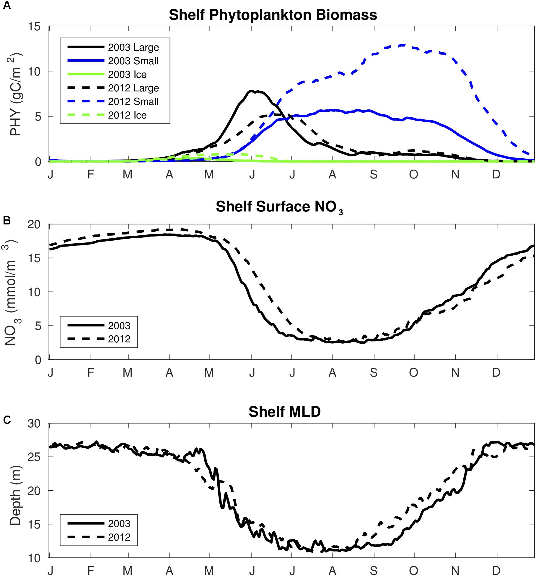
Figure 13. Time series plots of area-weighted spatial mean (A) 30 m column integrated phytoplankton biomass, (B) surface NO₃^-, and (C) mixed layer depth for model year 2003 and 2012. Phytoplankton biomass is divided into the large phytoplankton (black line), small phytoplankton (blue line), and ice algae (green line) functional groups.

The strengthening of this fall phytoplankton bloom is also the primary mechanism behind the ∼10 TgC/year increase in total carbon uptake from 2003 to 2012. This is a substantial increase in total carbon uptake over only a 10-year timeframe, though we note that this change equates to approximately one-sixth of the total variability between the various observationally based estimates for Bering Sea shelf carbon uptake. Comparing Figures 9, 10 illustrates that the increase in carbon uptake is co-located with the increase in primary production in outer shelf regions. Colder water temperatures will also decrease pCO₂ values which can generate enhanced ocean carbon uptake by enhancing negative ΔpCO₂ values. Indeed, the regions of greatest increasing carbon uptake (i.e., the southeastern outer shelf) are located where both mechanisms (i.e., increased productivity and colder temperatures) are present. Though there is a slight decreasing trend in annual wind speed (∼0.05 m/s/year) through large portions of the coastal shelf, the trend is not statistically significant. The substantial increase in ice cover during the cold period can also impact shelf carbon uptake by further inhibiting air-sea exchange and by meltwater dilution of surface DIC and TA concentrations. The latter mechanism is evident by the freshening of the outer shelf waters during the cold period (Figure 9L), though the effect is not as apparent with DIC and TA. Implementing mechanistic connections between sea ice formation/melt and DIC and TA concentrations (e.g., Rysgaard et al., 2012) that are currently not included in our model may help resolve this connection for future work.

Previous studies have noted significant variability in temperature and sea ice extent between the 2003–2005 and 2010–2012 timeframes, which likely impacted the marine ecosystem (Stabeno et al., 2012). There is considerable debate regarding whether warmer water temperatures and reduced sea ice extent will increase or decrease primary productivity (Lomas et al., 2012; Brown and Arrigo, 2013; Eisner et al., 2014; Banas et al., 2016; Liu et al., 2016). In the Bering Sea, warmer years have been tied to reduced large copepod and euphausiid populations and subsequent weaker summer/fall lipid content and survival of age-0 walleye Pollock and Pacific cod recruits, which consume the copepods and euphausiids (Hunt et al., 2011; Mueter et al., 2011; Stabeno et al., 2012). However, this response is thought to be tied specifically to the strength of the spring diatom bloom supporting spring zooplankton populations (e.g., copepods and euphausiids) as opposed to annual net productivity. Our model results suggest that warmer years are less productive overall, though with slightly more productivity on the inner shelf. A similar response with zooplankton (i.e., warmer temperatures generating less zooplankton overall, but slightly more on inner shelf) was noted by Hermann et al. (2016) in climate change projections out to 2040 using the Bering10K model. Thus, we expect that the modeled increase in primary productivity from 2003 to 2012 is temporary and will revert to lower values with the return of warm conditions and future warming.

For this study, our primary interest in productivity stems from the biogeochemical connection to the carbonate system. An increase in productivity and carbon export can decrease surface DIC concentrations, and thereby mask the expected increase in surface DIC and corresponding decrease in Ω_Arag due to OA. However, shelf DIC increases at a rate similar to that expected due to increasing atmospheric CO₂ (Figure 12). This increase in DIC accounts for the rapid decrease in Ω_Arag, but it is perhaps less intuitive as to why the DIC is increasing at a rate comparable to the expected rate from increasing atmospheric CO₂, despite the increase in productivity. This discrepancy results from the composition (i.e., small phytoplankton) and fall timing of the increase in productivity. For instance, the cold period drives enhanced negative ΔpCO₂ values in fall due to colder water temperature and increased productivity. However, this productivity is in the form of small phytoplankton, which have a significantly slower sinking rate compared to large phytoplankton (0.05 m/day vs. 1.0 m/day, respectively). Thus, this organic carbon is not permanently buried (Figure 12D), but rather remineralized back to DIC during the winter and retained in the water column due to ice inhibition of air-sea exchange. This process combined with the increase in atmospheric CO₂ results in a net annual increase in DIC, despite the increased productivity.

It is possible that the model is overestimating the trend in productivity and thereby shelf carbon uptake, which would exacerbate the previously described mechanism. Ortiz et al. (2016) noted that model fall productivity is likely biased high, particularly due to strong small phytoplankton blooms. These fall blooms are further enhanced during the cold period, due to relatively deeper mixed layer depths and enhanced vertical transport of sub-surface nitrate. The colder period is also defined by a comparatively weaker spring diatom bloom, leaving more nitrate in the summer surface layer for small phytoplankton (Figure 13). Model surface DIC does not contain a significant bias though, suggesting a reasonable seasonal biological drawdown of carbon. Surface NO₃^- is the only model variable that displays much greater variability compared to the observations (Figure 3), though model NO₃^- is also biased somewhat high compared to the observations, which is not what we would expect if model productivity is biased high. Ammonium inhibition of nitrate uptake could also lead to the higher nitrate concentrations, though this process is modeled to prevent the complete limitation of nitrate uptake at high ammonium concentrations (Gibson and Spitz, 2011).

Over the 10-year model hindcast, statistically significant increasing trends in surface ocean DIC and pCO₂, along with a decreasing trend in Ω_Arag are apparent throughout most of the Bering Sea shelf. These are the long-term changes expected due to OA. That these trends emerge within a 10-year timeframe is surprising considering the highly variable coastal setting and substantial temperature variability. The transition from warm to cold water conditions acts to decrease surface ocean pCO₂ values, due to increased gas solubility and primary production. Yet, surface ocean pCO₂ values largely increase at a rate comparable to that expected due to increasing atmospheric CO₂ (Figures 11, 12). For pCO₂, the temperature driven signal and the atmospheric CO₂ driven signal act in opposition. Conversely, both colder water temperatures and increasing atmospheric CO₂ act to decrease Ω_Arag values. For Ω_Arag, the transition from a warm to cold regime acts to accelerate the decreasing trend. Comparing Figures 9C, 10C illustrates that the region of greatest temperature decrease in the southeastern middle shelf corresponds to the region of greatest Ω_Arag decrease. However, warm conditions returned to the Bering Sea starting in 2014 (Duffy-Anderson et al., 2017), thus this mechanism likely did not continue.

The Community Earth System Model (CESM) projects that, under RCP 8.5, annual average surface Ω_Arag will decrease by an additional 0.70 units by the end of the century and reach the saturation threshold (i.e., Ω_Arag < 1) by 2062 (Mathis et al., 2015a). If extrapolated forward in time, our model results suggest a faster timeline, with annual average Ω_Arag values < 1 by 2040. However, this estimate is highly uncertain due to the simplistic extrapolation method and likely biased by significant variability encapsulated within our model timeframe. Furthermore, observed and modeled spatial variability suggests that this timeframe may vary by up to several decades between different shelf regions. Future work will utilize ESM output to dynamically downscale OA projections using the Bering10K model (Hermann et al., 2016; Wallhead et al., 2017). This method will reduce the uncertainty of these critical threshold years and provide information on their spatial variance throughout the Bering Sea.

Conclusion

We use a regional model of the Bering Sea to illustrate how coastal biogeochemical processes and climate variability impact aragonite saturation state over a 10-year timeframe. Freshwater runoff from the Yukon River reduces surface Ω_Arag values to < 1 from December-May along the inner shelf region, particularly in Norton Sound. Conversely, substantial primary productivity increases Ω_Arag values to >2 along the outer shelf and shelf break regions, though Ω_Arag still decreases to ∼1.5 during winter months. A shift from relatively warm, low sea ice conditions (2003–2005) to relatively cold, high sea ice conditions (2010–2012) produces a significant increase in fall productivity and ocean carbon uptake throughout the outer shelf region. Surface DIC increases at a rate of 2.5–4.0 mmol/m³/year and surface Ω_Arag decreases at a rate of 0.025 – 0.04 units/year. These trends are statistically significant throughout most of the middle and inner shelf domains, though they are likely enhanced by the transition from the warm to cold period. Nonetheless, these trends are relatively greater than those observed for the open ocean, illustrating how high-latitude coastal shelf regions serve as hotspots of global change. Future work will utilize statistical downscaling to project these changes through 2100 in order to determine critical threshold years for persistent annual Ω_Arag undersaturation and variability in this projected change between the inner and outer shelf regions.

Author Contributions

DP and JM conceived the project. DP and DN were responsible for the model simulations, analysis, and producing the manuscript figures. JC provided the observational data. AH provided the model forcing fields. AH, SS, and GG provided guidance and support for model development. DP wrote the first draft of the manuscript. All authors provided feedback and contributed to the final manuscript.

Funding

Part of this research was performed while DP held a National Research Council Research Associateship award at the Pacific Marine Environmental Laboratory. Funding was provided by the NOAA Arctic Research Program and through the Joint Institute for the Study of the Atmosphere and Ocean (JISAO) NOAA Cooperative Agreement NA15OAR4320063 (2015–2020). Funding for DN was provided by the NOAA Hollings Scholarship Program. This is PMEL contribution number 4802 and JISAO contribution number 2018-0158. Model output data supporting the conclusions of this manuscript will be made available by the authors, without undue reservation, to any qualified researcher.

Conflict of Interest Statement

The authors declare that the research was conducted in the absence of any commercial or financial relationships that could be construed as a potential conflict of interest.

Acknowledgments

We would like to acknowledge high-performance computing support from Yellowstone (ark:/85065/d7wd3xhc) provided by NCAR’s Computational and Information Systems Laboratory, sponsored by the National Science Foundation. Use of the Yellowstone system was provided by a postdoctoral allocation for DP.

References

Banas, N. S., Zhang, J., Campbell, R. G., Sambrotto, R. N., Lomas, M. W., Sherr, E., et al. (2016). Spring plankton dynamics in the Eastern Bering Sea, 1971-2050: mechanisms of interannual variability diagnosed with a numerical model. J. Geophys. Res. Oceans. 121, 1476–1501. doi: 10.1002/2015JC011449

ORIGINAL RESEARCH article

Modeled Effect of Coastal Biogeochemical Processes, Climate Variability, and Ocean Acidification on Aragonite Saturation State in the Bering Sea

Introduction

Materials and Methods

Physical Model Description

Biogeochemical Model Description

Boundary Conditions

Model Skill Assessment

Model Hindcast Setup

Results

Model Performance

Seasonal and Spatial Patterns

Warm and Cold Regimes

Decadal Trends

Discussion

Conclusion

Author Contributions

Funding

Conflict of Interest Statement

Acknowledgments

References

This article is part of the Research Topic

People also looked at