Utilizing Eutrophication Assessment Directives From Transitional to Marine Systems in the Thames Estuary and Liverpool Bay, UK

Introduction

Coastal marine ecosystems have been impacted globally by a range of anthropogenic activities including elevated inputs of nutrients (Jickells, 1998; Conley et al., 2009; Rabalais et al., 2009). Inputs of nutrients from direct discharge of waste water and diffuse sources including agricultural runoff and atmospheric deposition have led to many regions experiencing eutrophication, which includes undesirable changes in the marine ecosystem including increased primary production, accumulation of organic matter and an associated decrease in oxygen concentration (Nixon, 1995, 2009; Cloern, 2001; Cloern and Jassby, 2010; Breitburg et al., 2018). Coastal eutrophication is likely to continue into the future due to the increasing use of fertilizers, discharge of human waste and hydrologic modifications, with these impacts exacerbated by the warming climate (Rabalais et al., 2009; Seitzinger et al., 2010; Paerl et al., 2014).

Humans have significantly altered the balance of the nitrogen (N) and phosphorous (P) cycles which has led to documented changes in riverine and coastal N:P ratios with potential consequences for marine phytoplankton communities, including altered species composition and reduced biodiversity (Turner et al., 2003; Philippart et al., 2007; Grizzetti et al., 2012; Paerl et al., 2014; Burson et al., 2016). Nutrient inputs to riverine and coastal systems may come from diffuse sources (e.g., agricultural run-off and atmospheric deposition) and point sources (e.g., sewage treatment and industrial discharge). Measures to reduce nitrogen and phosphorous inputs are frequently more successful at reducing a single source of nutrients via targeted policies rather than all nutrients and it is recognized that parallel reductions in both nitrogen and phosphorous inputs are required to reduce coastal eutrophication and the impacts associated with a changing nutrient regime (Conley et al., 2009).

In Europe, environmental directives exist for assessing the status of freshwater, coastal and marine environments. These include the Nitrates Directive (EC, 1991), Water Framework Directive (WFD, see EU, 2000) and more recently, the Marine Strategy Framework Directive (MSFD, see EU, 2008). Agreements on eutrophication assessments have also been made under the Oslo and Paris Conventions for the Protection of the Marine Environment of the North-East Atlantic (OSPAR, see OSPAR, 2013) and the Baltic Marine Environment Protection Commission-Helsinki Commission (HELCOM, see Andersen et al., 2011). These environmental frameworks are used for making harmonized assessments of marine eutrophication through the assessment of several key criteria which detail the cause and impact of increased nutrient delivery. Whilst each directive or process is different in terms of scope, assessment area and integration rules, there is a set of common indicators across all the directives. These common or “primary” indicators include dissolved inorganic nutrients, chlorophyll-a, phytoplankton abundance and dissolved oxygen to assess conditions relative to thresholds identifying an accepted ecological state (Devlin et al., 2007a, 2011; Foden et al., 2011; Tett et al., 2013). Each directive typically relates to the assessment of criteria within a set of geographical or political boundaries which do not always represent an ecological boundary. These geographical constraints can mean that assessments are not always coordinated across a river to coast continuum, making it difficult to align with a program of measures that can be developed through the river basin management plans (UK Gov, 2016).

Within the United Kingdom (UK), there are several national agencies with responsibility for collecting data and reporting on the assessment of coastal and marine environmental status under the requirements of the WFD, OSPAR Common Procedure (OSPAR CP) and the MSFD. To date in the UK, assessments under the WFD and OSPAR have been made separately based on geographically defined regions (Foden et al., 2011; UK National Report, 2017), which does not necessarily provide a coordinated assessment across a river basin. WFD assessments are carried out at a waterbody level, where waterbodies are differentiated by estuarine and coastal typologies. Specific reference conditions have been developed for each type of system where waterbody type is defined by characteristics including tidal range, mixing, exposure and salinity (Devlin et al., 2011). Waterbodies are typically estuarine or coastal areas and range from between 0.05 and 1,200 km². The OSPAR CP screens for problem, potential problem and non-problem areas. The full assessment under OSPAR CP is only applied to problem or potential problem areas. All WFD waterbodies are designated based on the WFD assessment criteria and processes. For the OSPAR CP reporting, a WFD waterbody that has been designated as moderate, poor or bad under the WFD assessment is designated as a problem area under the OSPAR CP. The WFD data used to make the initial WFD assessment is not included in the OSPAR assessment of the regional seas areas.

The aim of this work was to improve our understanding of the eutrophication status across the salinity gradient in two study areas that receive significant anthropogenic freshwater nutrients: the Thames estuary and Liverpool Bay in England, by reporting individual criteria that are common to both WFD and OSPAR, and by exploring the outcomes of these criteria across several different assessment areas. The Thames and Liverpool Bay marine area catchments differ in terms of their geology, agriculture, population and land-use, resulting in different patterns of nutrient discharge. Both have historically received significant anthropogenic nutrient inputs. The primary indicators of eutrophication were applied to alternative ecologically relevant typologies in addition to the WFD- and OSPAR-defined typologies to examine whether changing the geographical boundaries of the assessment areas alters the outcomes of the primary indicators. Metrics from both WFD and OSPAR were applied to the different assessment areas and tested over a 10-year period (2006–2015). The objective was not to repeat or test the recent WFD or OSPAR outcomes but to investigate the stability of the metrics as the assessment areas are shifted into more ecologically relevant areas. Additional reporting of state was also tested by the inclusion of community-based indicators through the assessment of the long-term change in functional phytoplankton life forms. The outcomes of the metrics were also used to improve understanding of the effects of anthropogenic nutrient loading across the river to marine continuum.

Materials and Methods

Study Areas

Two study areas were selected: Thames in the south east of England and Liverpool Bay in the north west of England (Figure 1). In the Thames catchment, the total farmed area is 1,398 × 10³ hectares, of which 12% is permanent pasture and 78% is arable land. In contrast, in the catchment area of Liverpool Bay, the total farmed area is 940 × 10³ hectares, of which 62% is permanent pasture and 21% is arable land (Defra, 2018). The remainder of farmed land in both catchments is used for dairy herds, pigs and poultry. This difference in agricultural land use contributes to different nutrient loadings between the two study areas. Both study areas also have large centers of population within their catchments. The population in the Thames River Basin District is over 15 million people (Environment Agency, 2018a) and it is nearly 7 million people in the North West River Basin District, which encompasses the Liverpool Bay study area (Environment Agency, 2018b).

FIGURE 1

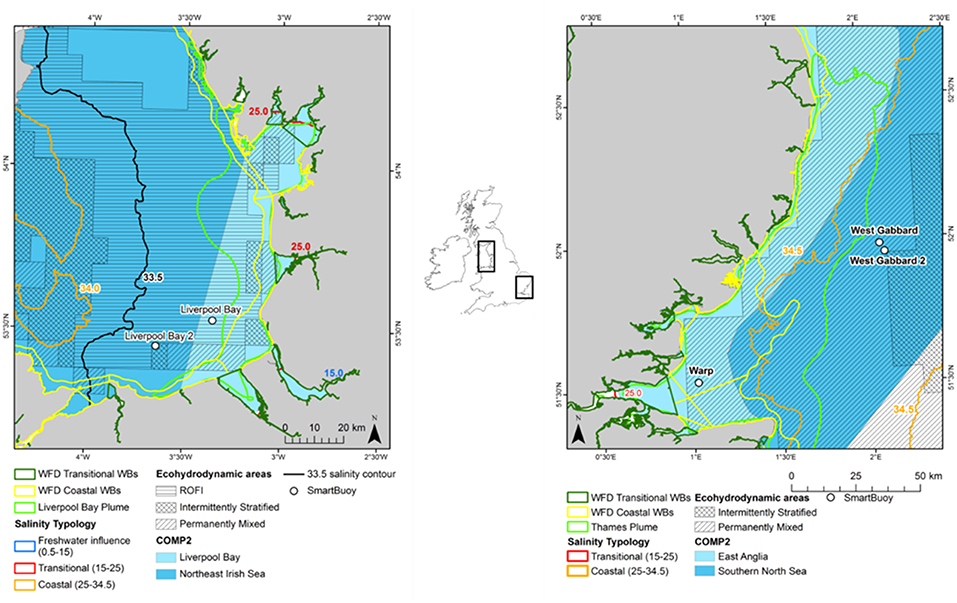
Figure 1. Location of the Liverpool Bay (left) and Thames (right) study areas with the typologies assigned.

Datasets

Datasets for salinity, dissolved inorganic nutrients, chlorophyll-a, suspended particulate matter (SPM), dissolved oxygen (DO) and phytoplankton community in the period from 2006 to 2015, which covered a range of spatial and temporal scales, were compiled from different sources (see Supplementary Table 1 for a summary) described in detail below. Trends in freshwater nutrient inputs were assessed between 1994 and 2016 as an indicator of long-term pressure on the two study areas.

Freshwater Flow and Inorganic Nutrient Loads

Riverine inputs of freshwater and inorganic nutrients for 1994–2016 were processed from raw data provided by the Environment Agency and the National River Flow Archive, with permission from the Welsh government to use the Welsh data from these datasets. Data for each river were calculated as the sum of river only loads plus direct sources (sewage plus industrial discharges) downstream of the last tidal gauge point. Loads were catchment corrected to account for ungauged areas. Further details are given in Lenhart et al. (2010) and van Leeuwen et al. (2015). Data for annual loads of nitrate, nitrite, ammonium, dissolved inorganic nitrogen (DIN) and dissolved inorganic phosphorus (DIP) were calculated. Dissolved inorganic nitrogen (DIN) was calculated by summing the concentrations of nitrate, nitrite and ammonium. Annual molar ratios of DIN:DIP were also calculated. Data from the following rivers were summed for each study area. Some rivers include late-joining tributaries (where the river is already tidal) or separate rivers that join in the estuary. Some rivers have data for flow only and not nutrient loads. This detail is included in brackets as necessary after the river name.

Thames: Thames (Beam, Beverley Brook, Brent, Crane, Ingrebourne, Lee, Mardyke, Ravensbourne, Roding, Thames, and Wandle), Chelmer (Chelmer and Blackwater), Colne, Medway, Stour, Deben (flow only), Alde (Alde and Ore, flow only).

Liverpool Bay: Clwyd (Clwyd and Elwy), Alt, Conwy, Dee, Derwent, Douglas, Ethen (flow only), Ellen (flow only), Esk (Esk and Lyne), Kent (Kent and Beela), Leven, Lune, Mersey, Ribble (Ribble and Darwen), Weaver, Wyre.

The yearly trends in the nutrients from both Liverpool Bay and Thames were assessed using Generalized Additive Models (GAMs, Wood, 2006), fitted by restricted maximum likelihood. This approach was adopted because the trends are not all linear and so a method that could fit more flexible trends was needed. The fit of the GAMs is shown in Supplementary Figure 1 for Thames estuary and Supplementary Figure 2 for Liverpool Bay. The statistical significance of the trend was assessed using a likelihood ratio test against the null model of no trend. The residuals from the GAMs were checked for temporal autocorrelation by plotting the empirical autocorrelation function for various lags and comparing this with the values expected if the series was uncorrelated. The residuals from these models did not exhibit any autocorrelation and so uncorrelated GAM models were used.

Ship Based Sampling—Estuarine to Coastal

Samples were usually collected at 2 m depth using a CTD. The sites are well mixed and samples from 2 m depth are considered to be representative of the surface water. Samples were filtered for inorganic nutrient analysis (nitrate, nitrite, ammonium, phosphate and silicate), chlorophyll-a and SPM. Salinity and dissolved oxygen were determined using YSI handheld conductivity and oxygen meters. Details of sample collection and analysis are given in Kennington et al. (1999).

Ship Based Sampling—Coastal to Offshore

Samples were collected using Niskin bottles mounted on a CTD rosette and from the non-toxic pumped supply on research vessels for the years 2006–2015. For Liverpool Bay, research cruises occurred, on average, eight times per year between 2006 and 2011 and on average six times per year from 2012 onwards. For Thames, research cruises occurred, on average, eight times per year between 2006 and 2013 and on average four times per year from 2014 onwards. In addition, samples were collected on other ad hoc research cruises in both study areas. Details of sample analysis and quality assurance for dissolved inorganic nutrients are given in Gowen et al. (2002). Methods for the analysis of dissolved oxygen, suspended particulate matter, chlorophyll-a and salinity are given in Greenwood et al. (2010).

SmartBuoy

Instrumented moorings (“SmartBuoy”) have been deployed in the Thames region and Liverpool Bay since 2000 and 2003 respectively (see Supplementary Table 2 for details). The instrumentation, parameters measured and methods are described elsewhere (Weston et al., 2008; Greenwood et al., 2010). Daily average values for salinity, SPM, chlorophyll-a and DO were calculated from 10-min burst measurements made every half an hour over a 24-h period. Total oxidized nitrogen (TOxN) was measured between every 2 h and every 4 days depending on the instruments deployed. Data for total oxidized nitrogen (TOxN), chlorophyll-a, DO and phytoplankton species composition and abundance were used in this study. Seven-day average values were calculated as SmartBuoy data is temporally correlated with a range of approximately 7 days (Capuzzo et al., 2015). Ammonium (NH₄) is not determined on SmartBuoy, therefore DIN was set equal to TOxN. Historical data from CTD and underway samples at these locations for November to February (the assessment period for nutrients) show that TOxN accounted for 97% of DIN at the Thames SmartBuoy and 86% of DIN at the Liverpool Bay SmartBuoy between 2006 and 2015.

Phytoplankton

Water samples (150 ml) were collected on SmartBuoys using automated water samplers into pre-spiked bags containing acidified Lugol's iodine. Samples were collected weekly and returned for analysis at Cefas when moorings were recovered every 1–3 months. Samples were decanted from the sample bags into 175 ml glass jars and topped up with 1 ml of acidified Lugol's iodine. A minimum of one sample per month was selected for analysis from each deployment location where sample availability allowed. Samples were analyzed at Cefas using the Utermöhl method (Utermöhl, 1958) under inverted Olympus IX71 microscopes within 1 year of collection. Species were identified and enumerated in the samples and counts recorded in cells per liter.

Since the inception of WFD monitoring from late 2006, Environment Agency (EA) phytoplankton samples have been collected from sites in WFD waterbodies from a combination of Coastal Survey Vessels, rigid hulled inflatable boats (RIBs), and rarely from jetties or bridges in estuaries (Devlin et al., 2012). The frequency of sampling in WFD transitional and coastal waters is typically one sample per calendar month from 3 to 5 sites per water body. Ideally, samples should be 28–31 days apart throughout the year. There must be at least a 14-day interval between sampling occasions at each site. The phytoplankton samples are collected from the mixed surface layer usually between 1 and 2 m below the water surface using a standard NIO/Niskin-style water sampler, avoiding the surface film and without disturbing bottom sediments. In coastal waters or non-turbid waters >5 m depth, where the diurnal vertical migration of phytoplankton with light availability must be accounted for, samples for phytoplankton were mainly collected during daylight hours. However, for some samples, the use of integrated depth sampling using a Lund-type tube system negated the need to constrain the sampling window to daylight hours.

Samples of 250 ml volume were collected in clear PET bottles filled to approximately 90%, leaving sufficient headspace to allow for preservation and homogenization. Samples were preserved with acidified Lugol's iodine, stored in the dark, ideally at a temperature of 3°C ± 2°C for no longer than 6 months. The samples were analyzed using the Utermöhl method (Utermöhl, 1958) under inverted microscopes. Analysis was conducted at Cefas until 2013 then at both Cefas and an external laboratory from 2013 onwards. One in every 30 samples was analyzed by multiple analysts as a check for quality assurance and inter-analyst comparability.

Satellite Suspended Particulate Matter

Spatially gridded (1.1 km resolution) monthly averages (from daily images) of non-algal Suspended Particulate Matter (SPM) were downloaded from the Cefas Data Hub (doi: 10.14466/CefasDataHub.31). This is an interpolated and merged dataset from SeaWiFS, MODIS, MERIS and VIIRS satellite sensors. SPM was derived using the Ifremer OC5 algorithm (Gohin, 2011) and full processing details are given in Cefas (2016).

Biogeochemical Model (Thames Only)

Data for nitrate, phosphate, chlorophyll-a, salinity and DO were extracted from the Cefas 50-year hindcast of the North Sea (using the GETM-ERSEM-BFM model) covering 1958–2008 as described in van der Molen et al. (2014) and van Leeuwen et al. (2013, 2015) with an extension of the hindcast run to 2010.

Assessment Areas

The assessment areas tested in this work come from several sources including the WFD typologies for transitional and coastal waterbodies defined under (EC, 2003) and the coastal and offshore areas described in Foden et al. (2011) for the 2009 OSPAR comprehensive assessment (COMP2). The WFD waterbodies are split into coastal and transitional waters with transitional waters defined as ‘bodies of surface water in the vicinity of river mouths which are partly saline in character as a consequence of their proximity to coastal waters, but which are substantially influenced by freshwater flows' (EC, 2003). WFD Coastal waters are defined as mean ‘surface water on the landward side of a line, every point of which is at a distance of one nautical mile on the seaward side from the nearest point of the baseline' (EC, 2003). These waterbodies represent the classification and management unit under the WFD assessment approach.

In addition to these typologies, an additional three typologies defined using ecological and bio-physical characteristics were investigated, including (i) eco-hydrodynamic areas, (ii) salinity-derived areas and (iii) river plume-influenced areas. The typologies were created using ArcGIS 10.5 and exported as shapefiles. The open-source language R and environment were used to assign typologies to the input datasets (R Core Team, 2017). The resulting assessment areas are shown in Figure 1. Note that the offshore areas used in COMP2 (Southern North Sea in Thames and Northeast Irish Sea in Liverpool Bay) extend beyond the areas considered in this study (Foden et al., 2011).

Ecohydrodynamic Areas

Ecohydrodynamic regions were identified as five distinct hydrodynamic regimes, based on stratification characteristics from the results of a 51-year simulation (Thames) and a 15-year simulation (Liverpool Bay) using the coupled hydro-biogeochemical model GETM-ERSEM-BFM. The five regimes are as follows: permanently stratified, seasonally stratified (not applicable for the areas of interest in this study), intermittently stratified, permanently mixed and region of freshwater influence, or ROFI (van Leeuwen et al., 2015; Figure 1).

Salinity-Derived Areas

Salinity was used to define additional assessment areas given its importance in determining physical conditions, biological processes and a useful proxy to define riverine influence (Foden et al., 2008). A combination of Cefas and EA ship data selected between 2006–2016 and 0.5–35.5 salinity were used to interpolate a salinity surface. Since the combined salinity dataset was autocorrelated but not normally distributed and salinity was expected to be similar locally, the Inversed Distance Weighted (IDW) interpolation was selected (Stachelek and Madden, 2015). The sensitivity analysis on the IDW input parameters was conducted using a cross-validation dataset (10% of the input dataset), and the surface with the lowest root-mean-square error and absolute error was chosen. The interpolated salinity surface was divided into three regions. The area for the region of freshwater influence (ROFI) and a salinity range between 0.5 and 15 was 2.3 km² and 0 km² for Liverpool Bay and Thames, respectively. The area for transitional waters was selected based on a salinity range between 15 and 25 and covered 108 km² for Liverpool Bay and 34 km² for the Thames. The area for coastal waters was selected based on a salinity range between 25 and 34.5 and covered 10,820 km² for Liverpool Bay and 4,809 km² for the Thames.

River Plume-Influenced Areas

The riverine plume assessment areas for Liverpool Bay and Thames were defined by the extent of the riverine-influenced turbidity. Whole river plumes were defined based on the mean satellite SPM between 2006 and 2015. Transects at 10 km intervals running from the coast toward the sea were plotted to identify the steepest gradient in SPM with distance from the coast as an estimate of the extent of the river plume. The value of SPM at the point of steepest gradient was extracted (25 mg l⁻¹ for Thames and 10 mg l⁻¹ for Liverpool Bay). This threshold was used to map out the influence of the Thames and Liverpool river flow from the mean satellite SPM. The areas designated as plume using this method are 5,724 km² for Thames and 1,792 km² for Liverpool Bay (Figure 1).

Assessment Methods

The primary indicators for eutrophication, DIN, DIP, chlorophyll-a and DO and the secondary indicator of phytoplankton abundances (counts) were applied over each assessment area, where there were sufficient data for each parameter. Data limitations meant that not all indicators could be run for all assessment areas. The indicators followed the OSPAR harmonized criteria (Malcolm et al., 2002; Foden et al., 2011; UK National Report, 2017) and the WFD nutrient (Devlin et al., 2007b) and marine plant assessment tools (Best et al., 2007; Devlin et al., 2007c, 2012). Data were divided into three salinity ranges; transitional (<30), coastal (Thames 30–34.5, Liverpool Bay 30–34) and offshore (Thames ≥ 34.5, Liverpool Bay ≥ 34) according to Foden et al. (2011). All available data from all sources were pooled in calculations. We recognize that in some cases this may bias results toward more temporally or spatially rich data sources, an important issue that relates to data aggregation which is the focus of future research.

Degree of Nutrient Enrichment

A flowchart showing the processing steps for nutrients is given in Supplementary Figure 3. The assessment procedures followed UK National Report (2017) for OSPAR and Devlin et al. (2007b) for WFD. DIN and DIP data were selected for the winter assessment period from November to February, inclusive using data for the whole water column. Observations with corresponding salinity < 5 were excluded based on the WFD method. Data for DIN in the transitional range were normalized based on their salinity classification to salinity 25 (transitional), salinity 32 (coastal) and salinity 34.5 (Thames offshore) or 34 (Liverpool Bay offshore). This process involved fitting a linear regression to the DIN vs. salinity relationship for all data within each region and using that regression to determine the expected DIN at the normalization salinity. The OSPAR assessment of DIN was calculated as the normalized mean of all data for each assessment year. The mean was compared with the appropriate threshold; transitional waters (30 μmol l⁻¹), coastal waters (18 μmol l⁻¹) and offshore waters (15 μmol l⁻¹).

Under WFD, the assessment of DIN for transitional and coastal waters is modified where suspended particulate matter (SPM) was >10 mg l⁻¹. If the threshold was exceeded, the 99th percentile of salinity-normalized DIN was calculated. Waterbodies were classified by SPM as intermediate (10 < SPM < 70 mg l⁻¹), turbid (70 < SPM < 300 mg l⁻¹) or very turbid (>300 mg l⁻¹), dependent on the mean annual SPM. The 99th percentile threshold value was calculated from a sliding scale between these three conditions of SPM and the maxima (99th percentile) value of annual DIN; 70, 180, and 270 μmol l⁻¹ for intermediate, turbid and very turbid waters, respectively.

To provide the OSPAR assessment, the annual value of mean salinity-normalized DIN for each assessment year is reported as above (+) or below (–) the threshold or identified as insufficient (?) where there was not enough data to calculate a mean. The overall assessment for the 10-year period was made by summing the result for each individual year and assigning a color indicating predominantly above or below thresholds in the results table (Table 1). The WFD assessment of DIN was made in the same way as for OSPAR but data for all 10 years were pooled to calculate a single mean salinity-normalized DIN. This was compared to the same thresholds as for the OSPAR assessment of DIN. The thresholds used for the WFD assessment of DIN are the boundaries between good and moderate status (Devlin et al., 2007b).

TABLE 1

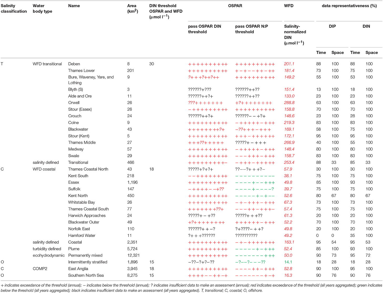
Table 1. Summary of outcomes for nutrient assessment tools for Thames estuary.

The OSPAR assessment of DIN:DIP was made by calculating the molar ratio of all co-observed DIN and DIP data between November and February inclusive for each assessment year. The ratio was compared to the thresholds of >8 and <24 for all salinity ranges. The individual year assessments were combined as for the assessment of DIN.

Phytoplankton (Chlorophyll-a and Phytoplankton Counts)

The assessment procedures followed UK National Report (2017) for OSPAR and Devlin et al. (2007c) for WFD. Flowcharts showing the processing steps for chlorophyll-a and phytoplankton are given in Supplementary Figures 4, 5. Assessment of coastal and offshore waters was applied in the growing season from March to October, inclusive. In contrast, assessment of transitional waters was applied to the full year. For the OSPAR assessment of phytoplankton, only chlorophyll-a was considered. The chlorophyll-a assessment for coastal and offshore waters is the calculation of the 90th percentile of all growing season chlorophyll-a data and reported for each assessment year. This annual value is compared with the appropriate threshold; coastal (15 μg l⁻¹) and offshore (10 μg l⁻¹). Scoring for each year was the same as described for DIN. For the WFD (coastal) assessment of phytoplankton in coastal and offshore waters, the 90th percentile of all data between March and October was calculated for the entire 10-year period, with data first averaged monthly. This single value was compared to the assessment threshold of 15 μg l⁻¹. The chlorophyll metric was then combined with the WFD phytoplankton outcomes.

For the WFD coastal metric, the percent of all taxa counts >10⁶ cells l⁻¹ and the percent of chlorophyll-a observations >10 μg l⁻¹ were calculated. The mean of these two values was calculated and a re-scaled metric from 0 to 1 was calculated based on the percent exceedance (Devlin et al., 2007a). The percentages of diatoms and dinoflagellates below a certain monthly reference were determined. The mean of these two values was calculated and a re-scaled metric from 0 to 1 was calculated based on the percent exceedance. The 90th percentile chlorophyll-a concentration was re-scaled to give a value between 0 and 1. The mean of these three metrics was calculated and compared to the WFD good-moderate boundary of 0.6.

The WFD transitional assessment is similarly composed of chlorophyll-a and phytoplankton counts components. A chlorophyll-a multi-metric for different statistical measures was determined (Devlin et al., 2007c) by splitting the data into two salinity ranges (5–25 and 25–30) and then calculating the following 5 metrics, with corresponding thresholds given in brackets: mean (<15 μg l⁻¹) and median (<12 μg l⁻¹) chlorophyll-a concentrations, and the percent of observations <10 μg l⁻¹ (>70%), <20 μg l⁻¹ (>85%) and >50 μg l⁻¹ (<5%). These calculations used monthly averaged values. For each of the 5 thresholds that was not exceeded in each salinity class with observations from at least 10 months of the year, a score of 1 was assigned, with the final score being the average over the 5 or 10 metric components depending on if both high and low salinity data are available. The resulting 0–1 metric was not compared with a threshold but was combined with the phytoplankton assessment.

The WFD transitional phytoplankton counts metric is composed of two components, the percent of counts for all taxa (combined) exceeding 10⁶ cells l⁻¹ and the percent of counts for any one taxa exceeding 500,000. Both metrics were assessed against a threshold of <20%. A re-scaled metric from 0–1 was calculated based on the percent exceedance (Devlin et al., 2007c). The mean of this phytoplankton metric and the chlorophyll-a metric above were calculated and compared to the WFD good-moderate boundary of 0.6.

Dissolved Oxygen

A flowchart showing the processing steps for DO is given in Supplementary Figure 6. The OSPAR assessment for DO was made for coastal and offshore waters. Data were filtered for the stratification assessment period (July to October inclusive) and only data from within 10 m of the seabed were used. The mean of the lowest quartile of DO was calculated for each assessment year and compared with the threshold >6 mg l⁻¹. Scoring for the 10-year period was carried out as for DIN.

The WFD assessment for DO was made for transitional and coastal waters. Data for the whole year from within 10 m of the surface were used. The 5th percentile DO was calculated for the whole 10-year period. For coastal waters this was compared with the threshold >4 mg l⁻¹. For transitional waters, this was compared with a variable threshold > 0.0286*salinity + 5 mg l⁻¹. The threshold used for the WFD assessment of DO is the boundary between good and moderate status (Best et al., 2007).

A comparison of the OSPAR and WFD assessment methods for each indicator is provided in Supplementary Table 3.

Representativeness of the Data

Confidence in assessment results was investigated, in part, by the representativeness of the data for each parameter as used in the assessment calculations over the 10-year assessment period and the spatial extent of each typology. The calculation of spatial and temporal representativeness followed García-García et al. (2019) which is a modification of the method described by Brockmann and Topcu (2014). The spatial representativeness was assessed by dividing the assessment area into 0.12° (latitude and longitude) grid cells (approximately 10 x 10 km grid) as described in the UK National Report (2017). For some of the smaller WFD regions, this coarse resolution means that they are composed of only one grid cell, which was deemed appropriate for the purposes of comparison to larger areas; a finer scale would have required different-sized grid cells based on the size of the assessment region and in consideration of the monitoring program's sampling density. The width of the temporal intervals for the calculation of the temporal representativeness was set to 1 month following the UK National Report (2017) and which is in line with the WFD monitoring schedule. The representativeness was calculated by determining the number of temporal intervals or spatial grid cells in which observations were available and dividing by the maximum possible temporal intervals within that assessment or spatial grid cells whose centers fell within the assessment area. This method is more conservative than that of Brockmann and Topcu (2014), who assigned a non-zero representativeness to intervals without observations based on the size of the data gap and the steepness of the gradient of nearest available data.

Plankton Index Tool

Phytoplankton taxa names were matched to biological trait information (Tett et al., 2007, 2008) and analyzed using the Phytoplankton Index (PI) method (e.g., Whyte et al., 2017) in Matlab (Tett, 2016). Briefly, lifeform data at monthly temporal resolution are corrected for a zero value and log transformed [log (counts + z)] and plotted against one another. For diatoms z is set to 70 cells l⁻¹ and for dinoflagellates, z is set to 700 cells l⁻¹, which approximate the limits of detection as determined when analyzing a subsample of the original sample volume. The distribution of data during a “reference period” in lifeform-lifeform space is used to define a “reference envelope” containing 90% of observations. The plankton index for any comparison dataset is then calculated as the ratio of the comparison data points which fall within the reference envelope in lifeform-lifeform space to the total number of compared points. A PI value of 1–0.9 thus represents no change from the reference period, while a PI of 0 indicates no similarities between the two observation periods. For this study the reference envelope was defined using data from the final 3 years of the assessment period: 2013–2015. PI values for the years 2006–2012 thus report on the degree of change from the selected reference period. The diatom-dinoflagellate pairing is considered in this study, referred to as lifeform 1 (LF1).

Results

Changes in Freshwater Inputs

Freshwater nutrient loads to the Thames marine area are dominated by the rivers Thames (79.3% of total riverine DIN load and 83% of total riverine DIP load) and Medway (13.6% of total riverine DIN load and 10.6% of total riverine DIP load). Together they contribute 93% of total riverine DIN and 94% of total riverine DIP loads to the study area. In Liverpool Bay, the river Mersey contributes the greatest proportion of riverine DIN load (36%) and riverine DIP load (47%) but there are also significant contributions from the rivers Ribble, Dee, Weaver, Douglas and Clwyd. Together these six rivers contribute 82% to riverine DIN load and 89% of riverine DIP load to Liverpool Bay.

There are large variations in annual freshwater discharge and inorganic nutrient loads to the Thames estuary and Liverpool Bay (Figures 2A, 3A). Between 1994 and 2016, mean freshwater discharge to Liverpool Bay was 16.1 ± 3.0 × 10⁹ m³ y⁻¹ and ranged between 10.6 × 10⁹ m³ y⁻¹ and 21.8 × 10⁹ m³ y⁻¹. This is over three times greater than that to the Thames, which has a mean freshwater discharge of 4.8 ± 1.5 × 10⁹ m³ y⁻¹ with a range between 2.3 × 10⁹ m³ y⁻¹ and 7.6 × 10⁹ m³ y⁻¹. However, loads of DIN and DIP are similar between the two study areas. Loads of DIN to the Thames marine area ranged between 23,700 and 60,500 tones (Figure 2B) compared with between 35,800 and 58,500 tones to Liverpool Bay (Figure 3B). In both study areas, DIN is dominated by nitrate. Loads of DIP to Thames ranged between 2,700 and 8,000 tones (Figure 2B) compared with between 3,000 and 6,200 tons to Liverpool Bay (Figure 3B). There is strong seasonality in freshwater discharge and nutrient loads to both Thames and Liverpool Bay (Supplementary Figures 7, 8). Discharge and loads of DIN and DIP are greatest in December to February and lowest between June and September.

FIGURE 2

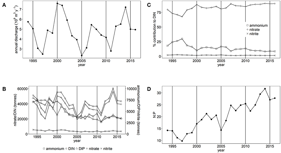
Figure 2. (A) Annual freshwater discharge, (B) Annual nutrient load, (C) % contribution of nitrate, nitrite and ammonium to DIN and (D) the molar N:P ratio for Thames study area.

FIGURE 3

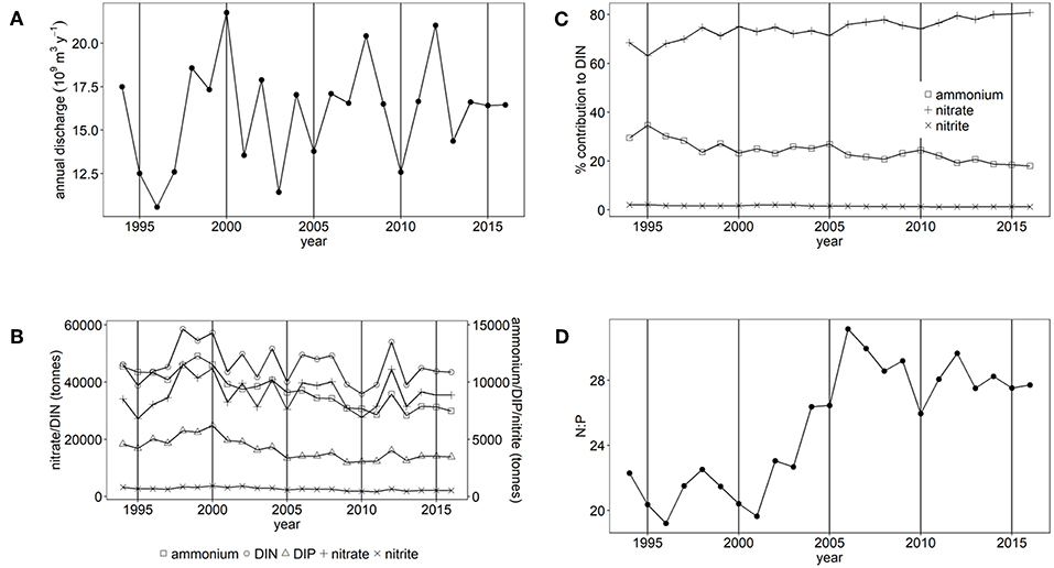
Figure 3. (A) Annual freshwater discharge, (B) Annual nutrient load, (C) % contribution of nitrate, nitrite and ammonium to DIN and (D) the molar N:P ratio for Liverpool Bay study area.

There have been statistically significant decreasing trends (p < 0.001) in the loads of ammonium, nitrite and DIP between 1994 and 2016 to both the Thames estuary and Liverpool Bay study areas (Figures 2B, 3B). There have been no statistically significant trends in loads of nitrate or DIN. Due to the decrease in ammonium loads, the percent contribution from ammonium to DIN has decreased from 30 to 9% in the Thames (Figure 2C) and from 35 to 18% in Liverpool Bay (Figure 3C). There has therefore been an increase in the percent contribution of nitrate to DIN from 68 to 90% in the Thames (Figure 2C) and from 63 to 81% in Liverpool Bay (Figure 3C). Nitrite contributes between 1 and 2% to DIN over the time period. The percent contribution to total nitrate from the six main rivers to Liverpool Bay (Mersey, Ribble, Dee, Douglas, Clwyd, Weaver) has changed over time. The annual nitrate load and therefore relative contribution from the Mersey has increased from 22 to 42% as the annual load and relative contribution from the other rivers has decreased. Nitrate loads show a strong correlation with average freshwater flow in the Thames estuary (Figure 4A, R² = 0.942, p < 0.001). The correlation between nitrate load and average freshwater flow is weaker in the Liverpool Bay study area (Figure 4B, R² = 0.642, p < 0.001).

FIGURE 4

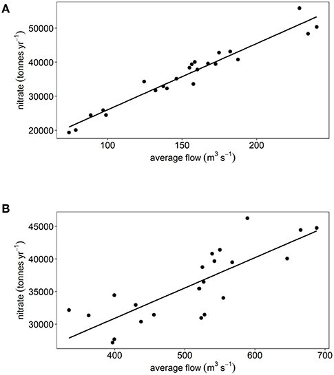
Figure 4. Annual nitrate load plotted against average flow rate for (A) Thames and (B) Liverpool Bay.

There has been a large and statistically significant increase (p < 0.001) in the ratio N:P in riverine loads to both the Thames estuary (Figure 2D) and Liverpool Bay (Figure 3D) since 1994 due to a larger relative decrease in P compared to N. In the Thames, N:P was a minimum of 9.8:1 in 1997, well below the Redfield ratio of 16:1, increasing to a maximum of 31.7:1 in 2006, well above Redfield ratio. In Liverpool Bay, the N:P ratio was a minimum of 19.2:1 in 1997, just above the Redfield ratio and reached a maximum of 31.1:1 in 2006, well above Redfield ratio. The statistical significance of the trends in nutrient loads and N:P to Thames and Liverpool Bay marine areas are summarized in Supplementary Table 4.

Application of the Assessment Indicators and Metrics

Outcomes Relative to Assessment Thresholds

In the Thames, all transitional assessment areas exceed the threshold for DIN (OSPAR and WFD) and N:P (OSPAR) (Table 1 and Figure 5). Salinity-normalized DIN ranges from 133.0 to 288.8 μmol l⁻¹. All coastal assessment areas exceed the DIN threshold under both the OSPAR indicator and WFD metric, with salinity-normalized DIN ranging from 38.1 to 67.3 μmol l⁻¹. The offshore assessment area ‘intermittently stratified' was below the thresholds for DIN (OSPAR and WFD) and N:P (OSPAR), with a mean salinity-normalized DIN of 14.1 μmol l⁻¹, but there was an insufficient amount of data for making an assessment for OSPAR DIN over this time period. The salinity-normalized DIN for the Southern North Sea assessment area was above the threshold for both OSPAR and WFD (16.3 μmol l⁻¹) but below the threshold for the OSPAR N:P indicator. The spatial representativeness is high in most assessment areas, with a few notable exceptions including the salinity-defined transitional area, Hamford Water DIP, salinity-defined coastal area and intermittently stratified eco-hydrodynamic area. The temporal representativeness is low for the intermittently stratified ecohydrodynamic area, variable in the WFD transitional and coastal assessment areas and high for the salinity-defined, turbidity-defined and ecohydrodynamic areas.

FIGURE 5

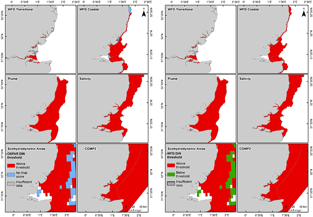
Figure 5. Outcomes for the OSPAR DIN assessment (left) and WFD DIN assessment (right) for Thames Estuary.

In Liverpool Bay, all transitional assessment areas (except two with insufficient data) exceed the OSPAR and WFD threshold for DIN (Table 2 and Figure 6) and all except one exceed the N:P OSPAR threshold. Salinity-normalized DIN ranges from 43.2 to 191.5 μmol l⁻¹. Seven of the 12 coastal assessment areas (one with insufficient data) exceed the OSPAR DIN threshold and eight of 12 exceed the WFD threshold. Salinity-normalized DIN ranges from 12.6 to 119.2 μmol l⁻¹. The spatial representativeness is high in all assessment areas. The temporal representativeness is more variable with lower values for some of the WFD transitional and coastal assessment areas.

TABLE 2

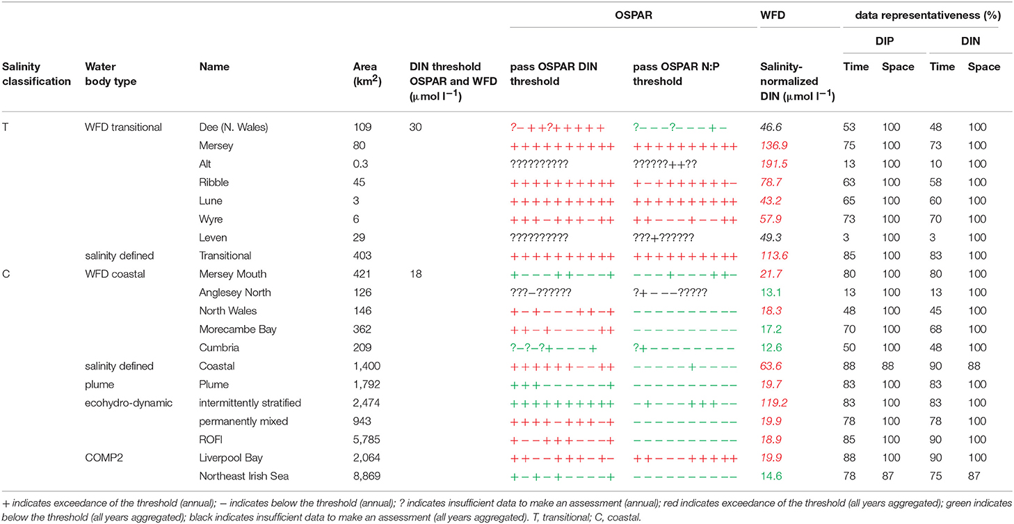
Table 2. Summary of outcomes for nutrient assessment tools for Liverpool Bay.

FIGURE 6

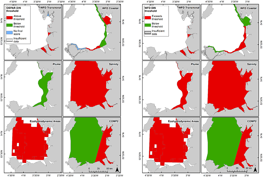
Figure 6. Outcomes for the OSPAR DIN assessment (left) and WFD DIN assessment (right) for Liverpool Bay.

The 90th percentile growing season mean chlorophyll for coastal assessment areas was below the threshold (15 μg l⁻¹) for all areas, ranging between 5.1 and 14.8 μg l⁻¹ (average 8.8 μg l⁻¹, Table 3 and Figure 7). Offshore areas were below the threshold (10 μg l⁻¹), ranging between 1.0 and 5.6 μg l⁻¹ (average 3.3 μg l⁻¹). One transitional area (Stour in Kent) was below the minimum threshold (0.6) for the combined chlorophyll + phytoplankton metric, with values for all other areas between 0.66 and 1.00 (average 0.87). All coastal and offshore assessment areas were greater than the minimum threshold for the combined chlorophyll + phytoplankton metric, with values for all other areas between 0.72 and 1.00 (average 0.87). The spatial representativeness for chlorophyll is high in all WFD assessment areas whereas the temporal representativeness is more variable. The spatial representativeness for phytoplankton is variable in the WFD assessment areas and higher than the temporal representativeness. The spatial and temporal representativeness for chlorophyll is reasonable in most of the salinity-defined, turbidity-defined and eco-hydrodynamic areas and greater than the spatial and temporal representativeness for phytoplankton.

TABLE 3

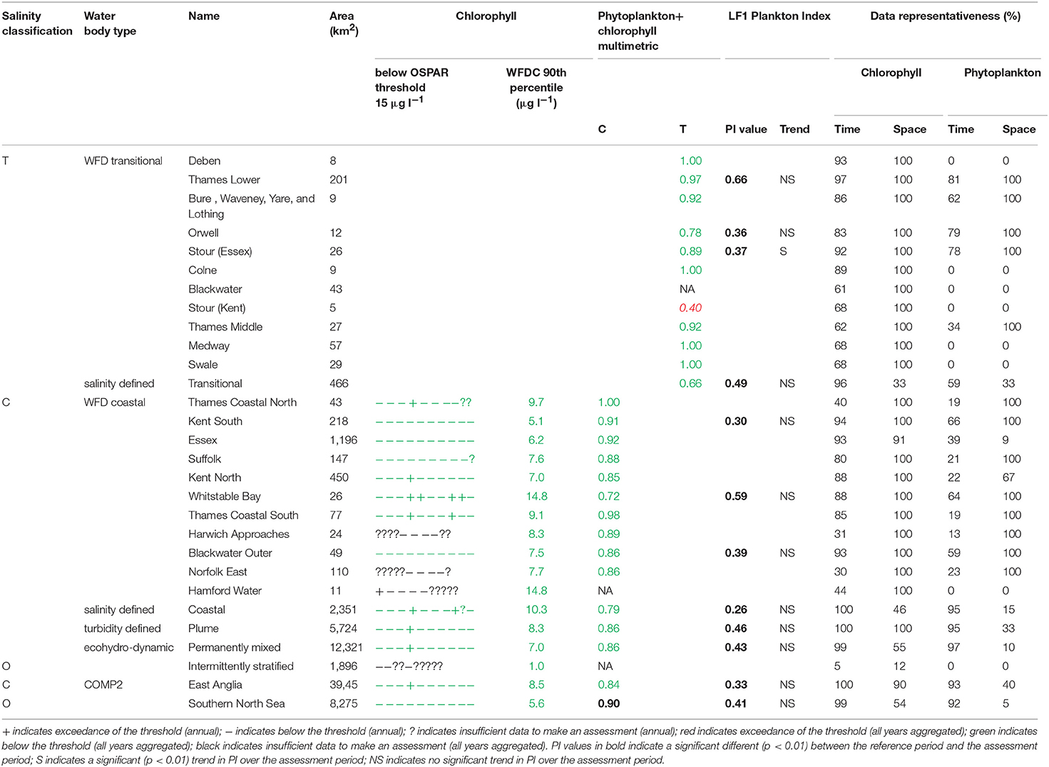
Table 3. Summary of outcomes for chlorophyll and phytoplankton assessment tools for Thames estuary.

FIGURE 7

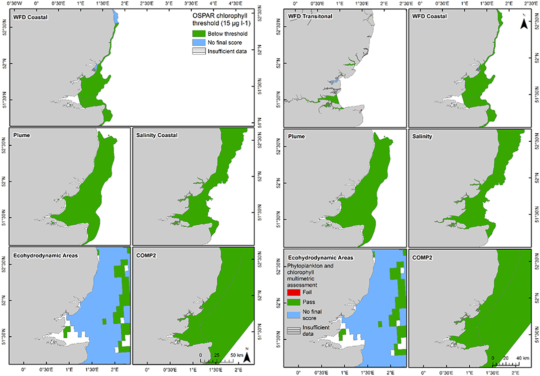
Figure 7. Outcomes for the OSPAR chlorophyll-a assessment (left) and WFD combined chlorophyll-phytoplankton assessment (right) for Thames Estuary.

Where there are sufficient data for PI values to be calculated, PI values for LF1 (diatom-dinoflagellate lifeform pairing) for all assessment areas show a statistically significant change (p < 0.01) due to increasing numbers of dinoflagellates in all assessment areas (Table 3). PI values for the four transitional areas assessed were between 0.36 and 0.66 (average of 0.47) and for the eight coastal and offshore areas were between 0.26 and 0.59 (average of 0.40). An example plot for the plume assessment area is shown in Figure 8, which is typical for all the assessment areas where there are sufficient data. Except for the transitional assessment area Stour (Essex), there was no significant trend in PI for LF1.

FIGURE 8

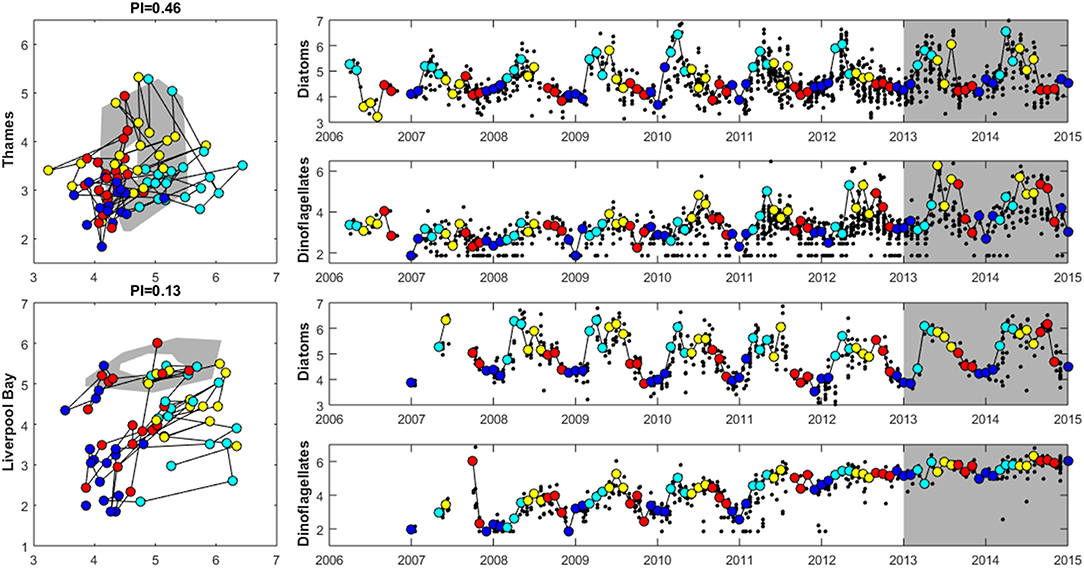
Figure 8. Plankton Index results for the Thames (top) and Liverpool Bay (bottom) plume typologies. The plots on the left show the data for 2006 to 2012 plotted compared to the reference envelope (2013–2015) in gray. The time series on the right show log10 (cell counts) for diatoms and dinoflagellates. Small black dots in the time series represent every observation, and the colored points (and line connecting them) match those in the PI diagram with colors indicating season: The reference period data (highlighted in gray in the timeseries) are not shown in the PI diagram. Dark blue: December–February, light blue = March–May, yellow = June–August, red = September–November.

In Liverpool Bay the 90th percentile growing season mean chlorophyll for coastal assessment areas was between 1.7 and 20.8 μg l⁻¹ (average 10.6 μg l⁻¹, Table 4 and Figure 9), with three of the coastal assessment areas (Mersey Mouth, salinity coastal and Liverpool Bay) exceeding both the OSPAR and WFD coastal chlorophyll thresholds (15 μg l⁻¹). In addition, Morecambe Bay exceeds the WFD coastal chlorophyll threshold. The results against the WFD combined chlorophyll + phytoplankton metric give very nearly the same result; the values for the combined metric for Morecambe Bay, salinity coastal and Liverpool Bay are below the minimum threshold of 0.6, while Mersey Mouth just exceeds the threshold with a value of 0.62. Across all coastal areas, values for the combined chlorophyll + phytoplankton metric ranged between 0.55 and 0.94 (average 0.74). In the transitional assessment areas, values of the combined chlorophyll + phytoplankton metric were between 0.27 and 0.89 (average 0.47), with six of the eight transitional assessment areas below the minimum threshold (0.6). The spatial representativeness for chlorophyll is 100% in all WFD assessment areas whereas the temporal representativeness is more variable. The spatial representativeness for phytoplankton is 100% in the WFD assessment areas except for three WFD coastal water bodies where there are no phytoplankton data. The levels of spatial and temporal representativeness for chlorophyll and phytoplankton are high in most of the salinity-defined, turbidity-defined and eco-hydrodynamic areas.

TABLE 4

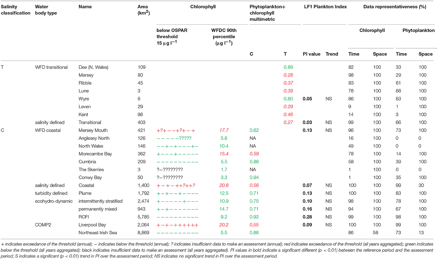
Table 4. Summary of outcomes for chlorophyll and phytoplankton assessment tools for Liverpool Bay.

FIGURE 9

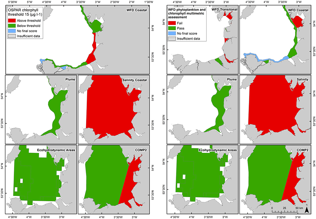
Figure 9. Outcomes for the OSPAR chlorophyll-a assessment (left) and WFD combined chlorophyll-phytoplankton assessment (right) for Liverpool Bay.

Where there are sufficient data for PI values to be calculated, PI values for LF1 (diatom-dinoflagellate lifeform pairing) for all assessment areas show a statistically significant change (p < 0.01) driven by increasing numbers of dinoflagellates in all typologies (Table 4). PI values for the two transitional areas assessed were between 0.03 and 0.05 (average of 0.04) and for the seven coastal areas were between 0.07 and 0.28 (average 0.14). An example for the plume assessment area is shown in Figure 8, which is typical of the other assessment areas where there are sufficient data. Lower PI values in Liverpool Bay indicate that changes in Liverpool Bay are greater than in the Thames. Across all assessment areas, the average PI for LF1 for Liverpool Bay is 0.12 compared to 0.42 for Thames. There were no significant trends in LF1.

In the Thames estuary, the 5th percentile DO concentrations (WFD metric) for the Thames (middle) and the transitional salinity assessment areas are below the oxygen minimum threshold (4.5 and 4.6 mg l⁻¹ respectively, Table 5). In all other transitional assessment areas, the 5th percentile DO concentrations are between 5.3 and 7.5 mg l⁻¹ (average 6.1 mg l⁻¹), greater than the minimum oxygen threshold. In coastal and offshore assessment areas, the 5th percentile DO concentrations are above the minimum threshold (4.0 mg l⁻¹), with values ranging between 6.2 and 8.0 mg l⁻¹ (average 7.0 mg l⁻¹) and the means of the lower 25th percentile (OSPAR indicator) are greater than the minimum oxygen threshold of 6 mg l⁻¹. The spatial representativeness for DO is high in nearly all WFD assessment areas whereas the temporal representativeness is more variable. The spatial and temporal representativeness for DO in the salinity-defined, turbidity-defined and eco-hydrodynamic areas assessment areas is variable, with low values for the Southern North Sea, intermittently stratified and salinity-transitional assessment areas.

TABLE 5

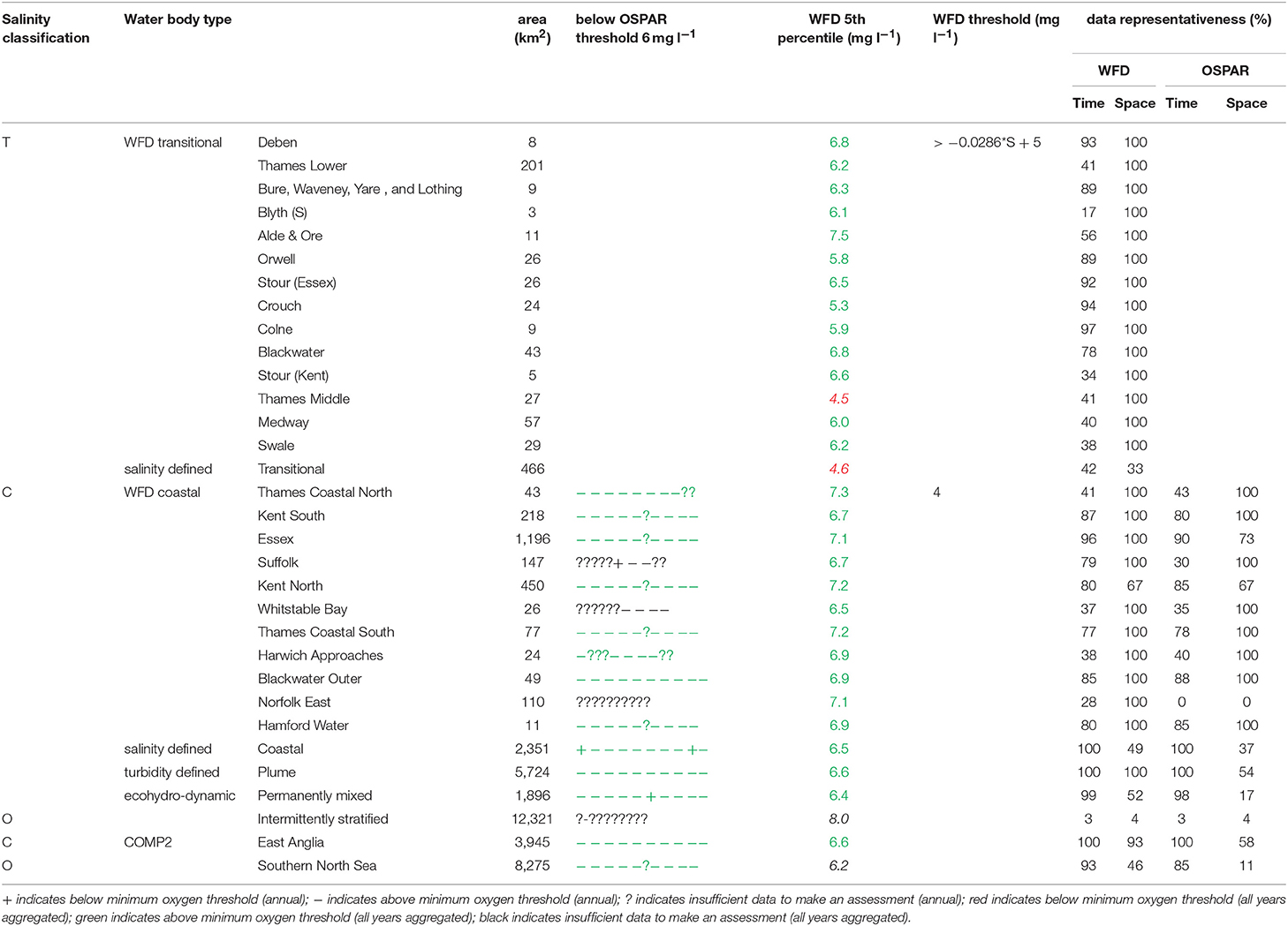
Table 5. Summary of outcomes for oxygen assessment tools for Thames estuary.

In Liverpool Bay, the 5th percentile DO concentrations and means of the lower 25th percentile are greater than the minimum oxygen thresholds in all assessment areas (Table 6). Values of 5th percentile DO concentrations were between 5.4 and 9.7 mg l⁻¹ (average 7.2) for transitional areas and between 6.5 and 7.5 mg l⁻¹ (average 7.0 mg l⁻¹) for coastal areas. The spatial representativeness for DO is 100% in all WFD assessment areas whereas the temporal representativeness is more variable. The spatial and temporal representativeness for DO in the salinity-defined, turbidity-defined and ecohydrodynamic areas assessment areas is mostly high apart from low spatial representativeness in the Northeast Irish Sea assessment area.

TABLE 6

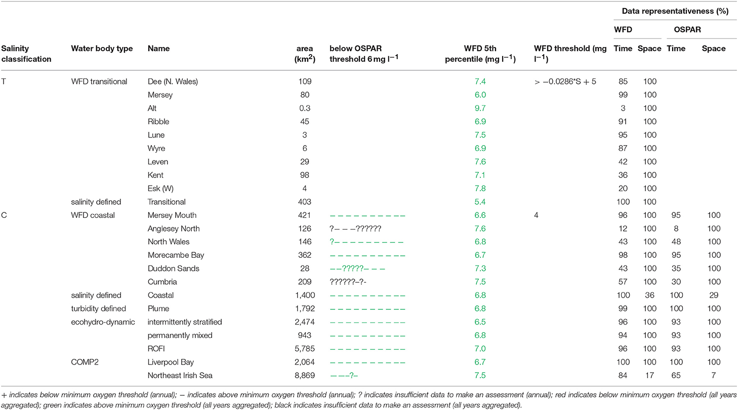
Table 6. Summary of outcomes for oxygen assessment tools for Liverpool Bay.

Comparison of Outcomes Between OSPAR and WFD Methods

Comparison of the WFD nutrient metric (aggregated over a 10-year period) with the reporting of the annual OSPAR primary nutrient indicators gave similar results for both Thames and Liverpool Bay despite the differences in temporal aggregation. The WFD nutrient metric is a salinity-normalized winter mean for the entire 10-year period. The OSPAR nutrient indicator is the same but assessed on 10 individual years and then reported as a final assessment based on the number of (non) exceedances for the 10-year period. In the Thames, there were some assessment areas with missing years where there were insufficient data to make an overall assessment against OSPAR DIN, but a value of WFD salinity-normalized DIN was always calculated for the entire 10-year period (Table 1). There were three notable differences in the DIN outcomes for Liverpool Bay where both Mersey Mouth and Liverpool Bay plume areas passed the OSPAR DIN assessment but exceeded the WFD salinity-normalized threshold. In contrast, Morecambe Bay failed the OSPAR DIN assessment but was below the WFD salinity-normalized threshold (Table 2).

The Thames coastal and offshore assessment areas have the same outcomes against the OSPAR chlorophyll indicator and the WFD phytoplankton metric (Table 3). The only differences were the assessment areas for where there was insufficient data to make an overall assessment against the OSPAR chlorophyll indicator. For Liverpool Bay, the outcomes against the OSPAR chlorophyll indicator, WFD coastal chlorophyll indicator and the WFD combined chlorophyll + phytoplankton metric were the same except for the Morecambe Bay assessment area (Table 4).

Outcomes for the coastal assessment areas in Thames and Liverpool Bay against the OSPAR DO indicator and WFD DO metric were the same, although different thresholds and different statistics were applied in the two assessment processes.

Discussion

Freshwater Nutrient Loads

Recent concerns about changing nutrient ratios (Turner et al., 2003; Philippart et al., 2007; Grizzetti et al., 2012; Paerl et al., 2014; Burson et al., 2016) highlight the impact of altered nutrient ratios on phytoplankton communities as a worldwide problem that needs to be considered in the future assessment of eutrophication levels in UK marine waters. Bowes et al. (2018) have shown that concentrations of phosphorous in the upper river Thames have decreased since 1997. These reductions are attributed to improved phosphorous stripping at sewage treatment works leading to reduced phosphorous loads from effluent rather than a reduction in agricultural inputs of phosphorous. A small reduction in nitrate was attributed to a reduction in diffuse sources such as agricultural inputs and not a reduction in nitrate load in sewage effluent. The changes in riverine nutrient loads observed in this study support the outcomes of these studies and highlight that policies targeted at reducing nutrient loads have led to significant decreases in DIP. However, there have been no significant decreases in DIN, particularly nitrate, and effective measures which also target reductions in nitrate are required to counter the significant increase in N:P observed.

The strong correlation between nitrate and river flow in the Thames (Figure 4A) suggests that nitrate sources to the Thames are dominated by diffuse sources (e.g., agricultural run-off). The correlation between nitrate and river flow is weaker in Liverpool Bay (Figure 4B). This may be because the nutrient load to Liverpool Bay comes from numerous rivers, the relative proportion of which have changed between 1994 and 2016. In addition, a mixed signal from point sources which are invariant with river flow (e.g., sewage treatment and industrial discharge) and diffuse sources such as agricultural run-off may lead to a weaker correlation between nitrate load and river flow.

Intra-annual Variability

The seasonal cycle in inorganic nutrients in the Thames displays maximum concentrations in the winter between December to March and a drawdown in April to June coincident with the documented spring bloom (Weston et al., 2008; Blauw et al., 2012). Concentrations of silicate reach a minimum before minimum concentrations of ToxN are observed. The PI analysis shows a strong seasonal cycle in the phytoplankton community abundance and composition at both study sites. Abundance is lowest at both sites in the winter months from December to February. The Thames shows a peak in diatom abundance in March and April, which generally decreases during June through November (Figure 8). Dinoflagellate abundance is greatest in May and June then decreases throughout the summer. The strong seasonal cycle in chlorophyll and the seasonal succession in phytoplankton community has been previously reported in Weston et al. (2008). Initially dominated by diatoms, the spring bloom then switches to dinoflagellates as silicate becomes limiting. After the spring bloom, diatoms dominate the lower summer phytoplankton biomass and microzooplankton play an important role in controlling phytoplankton growth during the summer (Weston et al., 2008). Blauw et al. (2012; Blauw et al., 2018) demonstrated that in the Thames, horizontal and vertical physical mixing processes driven by the tides are important in controlling phytoplankton concentrations at short time scales. At longer time scales of weeks to months, biological growth and loss processes driven by nutrients and light are important in controlling phytoplankton concentrations.

Previous studies have demonstrated that the seasonal cycle of winter maximum nutrient concentrations in February and drawdown in April/May in Liverpool Bay are recurrent features of this location, with the timing of the drawdown varying by several weeks between years (Foster et al., 1978, 1982a,b, 1983; Gowen et al., 2000; Greenwood et al., 2011, 2012). Concentrations of chlorophyll are low between November and March, peak in April and May and gradually decrease from June onwards. The PI analysis shows that diatom abundance is elevated between March and September with highest dinoflagellate abundances between May and September (Figure 8). Previous analysis has shown that at the Liverpool Bay SmartBuoy site the phytoplankton community is dominated by diatoms, with dinoflagellates most abundant between July and October each year (Greenwood et al., 2010, 2011). The variability in the underwater light climate and turbulent mixing are key factors controlling the timing of phytoplankton blooms.

Comparison of Outcomes From OSPAR and WFD Tools

Using nutrients, chlorophyll and dissolved oxygen is a good baseline for the assessment of eutrophication and, with appropriate thresholds, can provide a useful tool to assess the extent and impact of nutrient enrichment. The results of the assessments show that the current OSPAR and WFD assessment processes for eutrophication that are utilized in UK waters perform well in a cross comparison, showing similar outcomes from the application of the three primary indicators. Eutrophication in UK waters has typically been managed as a coastal issue, constrained to a small number of estuarine and coastal waters (WFD outcomes presented in UK National Report, 2017). Applying the primary indicators through both the WFD and OSPAR assessment approaches shows similar outcomes in the coastal assessment areas tested in this study. This is interesting given that the use of salinity and riverine plume-derived areas has extended the coastal areas beyond the one nautical mile of the coastal WFD typology. The estuarine assessment areas, which include both the WFD transitional waters and the salinity-defined estuarine area fail against the nutrient metrics under both assessment approaches, as would be expected in the heavily modified sub-catchment areas of the Thames estuary (Figure 5) and Liverpool Bay (Figure 6). The outcomes for the nutrient metrics in the coastal waterbodies are also similar between the WFD and OSPAR process. However, Harwich Approaches, Norfolk East and Hamford Water do have different outcomes between the WFD and OSPAR nutrient assessment, which is more a reflection of the limited data in several of the years than differences in assessment processes, highlighting the sensitivity of the assessments to data frequency. The salinity-defined coastal areas, the turbidity-defined plume, the ecohydrodynamic areas and the COMP2 assessment areas all have similar outcomes in the nutrient assessment, with nearly all the areas failing both the WFD and OSPAR nutrient assessment. The exception is the intermittently stratified areas, which pass the WFD nutrient assessment. The only assessment area that does not fail the nutrient assessment is the larger ecohydrodynamic areas, which reflects the larger offshore, less riverine-influenced area.

The chlorophyll metric could not be compared across the WFD and OSPAR metrics as only the WFD process has a chlorophyll metric for transitional waters. For the transitional assessment areas in the Thames, the chlorophyll metric only fails in one waterbody (Stour), reflecting the high turbidity and light-limiting characteristics of these eastern waterbodies. In contrast, the transitional assessment areas of Liverpool Bay have only two (out of eight) waterbodies (Dee and Wyre) that pass the chlorophyll sub-metric, reflecting the clearer waters with potential for higher phytoplankton growth (Cole and Cloern, 1987; Painting et al., 2007).

The coastal chlorophyll metrics for WFD and OSPAR include the assessment of the 90th percentile value of chlorophyll during the growing season. The OSPAR metric is based solely on the 90th percentile chlorophyll value whereas the WFD process has three sub-metrics: the 90th percentile chlorophyll value, phytoplankton counts and measures of seasonal succession of two major phytoplankton groups (diatoms and dinoflagellates). Despite the differences in the chlorophyll process, the comparison between WFD, OSPAR and salinity/turbidity-defined assessment areas shows similar outcomes for the Thames, with the assessment values not exceeding the thresholds in any coastal, salinity, plume defined or offshore areas (Figure 7). These non-exceedances represent the higher turbidity waters limiting phytoplankton growth, which can be seen in those lower values of biomass and abundances. These higher turbidity waters seem to extend further offshore into the larger coastal assessment areas. In Liverpool Bay there is also good comparability between results for the OSPAR and WFD chlorophyll assessments, apart from Morecambe Bay, which fails the WFD phytoplankton multimetric but not the OSPAR criteria. Interestingly, the salinity-defined coastal area (Figure 9) exceeds both the WFD and OSPAR criteria, suggesting that this larger assessment area would have a different outcome than the smaller WFD coastal areas. This may be due to decreasing turbidity in the salinity-defined coastal area, with increasing distance from the coast that permits greater phytoplankton growth and therefore elevated chlorophyll concentrations. In contrast, turbidity in the turbidity defined plume limits phytoplankton growth, and therefore chlorophyll concentrations are below the assessment threshold (Cole and Cloern, 1987; Painting et al., 2007).

The outcome for the dissolved oxygen assessment in transitional assessment areas shows that most of the transitional waters for Thames and Liverpool Bay do not fail the DO threshold. The exceptions are the Thames Middle transitional water and the salinity-defined transitional assessment area, which are similar areas and therefore have very similar results (Figure 1). The DO value for the salinity-defined transitional area in Liverpool Bay is lower than what is calculated for the individual WFD transitional waterbodies. This is because the salinity-defined transitional area is very coastal (Figure 1) and does not necessarily encompass the whole WFD transitional waterbodies and therefore only includes the very coastal subset of the WFD transitional data. The outcomes for the dissolved oxygen metrics are similar across the WFD and OSPAR criteria and are also similar across all the different assessment areas. The DO values calculated by the 5th percentile do change, with lower values in the transitional waters, increasing in all the coastal and offshore waterbodies.

To date in the UK, assessments made under WFD and OSPAR have not been integrated, and exceedances under the OSPAR assessment have not fed back into the program of measures under the WFD. However, assessments under the MSFD include WFD coastal waters and use some of the WFD tools for part of the assessment of Good Environmental Status, applied at a broader scale than an individual WFD water body. Therefore, in the future the WFD will provide support for the achievement of Good Environmental Status in marine waters. The thresholds used in the WFD and OSPAR assessments were developed at a time of limited data (prior to 2007). Given the advances in remote sensing, modeling and improved data collection, it is timely to consider testing of these thresholds to ensure they are still appropriate, such as is happening under the project JMP-EUNOSAT (Joint Monitoring Programme of the Eutrophication of the North Sea with Satellite data, 2017–2019). The UK chlorophyll threshold values were derived from the background nutrient concentration, assuming a constant Redfield C:N ratio and set C:Chlorophyll values (Foden et al., 2011). Recent research has shown seasonal variability in the uptake of carbon and phosphorous in shelf seas, which deviates from Redfield (Davis et al., in press; Poulton et al., in press). Therefore, reviewing the current chlorophyll thresholds in light of this recent research would be appropriate.

Additional Assessment Areas and Tools

The WFD transitional and coastal waterbodies are useful to flag issues at the fine spatial scale, and the smaller scale of these assessments is required to direct back to programs of measure and river basin management plans. Temporal representativeness is low in some cases, but this is expected given that they represent very small spatial areas. In the Thames estuary, the turbidity-defined plume assessment area is a large reporting area that represents the area of both the salinity-derived transitional and coastal assessment areas, and therefore represents one of the only fully integrated “catchment to coast” assessment areas. In Liverpool Bay, however, the plume assessment area includes the salinity transitional and only a fraction of the salinity coastal assessment areas. The additional process that reports across the salinity gradient, and fully encompasses the riverine influence of these large UK catchments, could provide an important component in understanding the links between river basins, land use information and downstream impacts. The smaller scale WFD waterbodies have been successfully used in identifying direct source impact, with the larger scale COMP2 areas providing a full assessment of any potential offshore issues. Both these processes could be improved by the addition of a more intermediate assessment area, providing information on the direct and diffuse nutrient loads and the full extent of these riverine loads and potential impact. In this paper we used turbidity to define such an intermediate assessment area. The Forel Ule (FU) scale is a color comparator scale used to classify the color of the oceans, regional seas and coastal waters. Remote-sensing algorithms have been developed to classify water bodies from satellite imagery (Wernand et al., 2013), and the FU scale could be used as a standardized way of defining the extent of riverine influence. In addition, ecosystem models can be used to track the extent of riverine influence on the marine environment (e.g., Figure 4 in Painting et al., 2013).

The outcomes of the lifeform tool (Tett et al., 2008; McQuatters-Gollop et al., 2019) show that the phytoplankton communities in many of the assessment areas have changed in relation to the diatom and dinoflagellate counts. Whilst many of the assessment areas show a change in the PI value, signifying a change between the reference period (2013–2015) and the assessment period (2006–2012), there is not a statistically significant linear trend over the assessment period. However, the counts of diatoms and dinoflagellates in the assessment areas show an increasing number of dinoflagellates in the last few years (see Figure 8). Whilst it is difficult to ascertain if a change in plankton community is a negative one, it does demonstrate that the more established primary indicators that measure biomass and abundances may not be measuring these more complex changes in the phytoplankton community. Future assessment of phytoplankton metrics could include these type of measures to improve our understanding of community changes as well as the more traditional eutrophication indicators.

A protocol is being developed by the wider research community to use PI values to identify key stressors (McQuatters-Gollop et al., 2019). Low PI values observed here, indicating changes in plankton community in terms of the diatom and dinoflagellate lifeforms, appear to be driven in Liverpool Bay by increasing counts of dinoflagellates, especially during winter months, and in the Thames by increasing summertime dinoflagellate counts. These changes appear consistent across the different typologies we explore, with low PI values calculated in all areas with sufficient data. The drivers of community change require further investigation, but likely include changing phytoplankton counts vs. biomass and cumulative pressures including temperature and eutrophication.

Conclusion

The outcomes of this study show that there have been significant reductions in loads to these two large UK catchments for some nutrients, particularly for phosphorus. However, the management of phosphorous has been more successful than management of diffuse nitrogen loads, reflected in the increasing nutrient ratios and a common problem facing many coastal waters in the UK, Europe and internationally. The range of tools or metrics available to assess the impact of these changing nutrient loads are explored in this paper and show a great degree of consistency in different approaches across the WFD and OSPAR process. Many criteria still show similar outcomes despite slight differences in aggregation. The testing of more ecologically appropriate areas, as defined by salinity or riverine plume influence also show a degree of consistency when applying the different assessment metrics. The use of riverine plume and salinity-derived areas do show that the coastal issues of high nutrients and elevated phytoplankton biomass can extend beyond the narrow WFD coastal areas and could be a useful approach for future assessments when looking across the full salinity continuum. Additionally, the use of the phytoplankton lifeform tool, whilst not a typical approach in the eutrophication assessment process, highlights the importance of understanding community change in relation to the long-term nutrient shifts and should also be considered as part of a future eutrophication assessment process.

Author Contributions

NG, MD, MB, LF, CG, AM, SvL and JB drafted the manuscript. NG, LF, CG, and AM analyzed the data. JB fitted the GAM models, and SvL processed the riverine data from raw archives.

Funding

The work was funded through Defra contract SLA25.

Conflict of Interest Statement

The authors declare that the research was conducted in the absence of any commercial or financial relationships that could be construed as a potential conflict of interest.

Acknowledgments

The authors would like to acknowledge all scientific and technical staff at Cefas, the EA, The National River Flow Archive (CEH) and Afbi for data collection and processing.

Supplementary Material

The Supplementary Material for this article can be found online at: https://www.frontiersin.org/articles/10.3389/fmars.2019.00116/full#supplementary-material

References

Andersen, J. H., Axe, P., Backer, H., Carstensen, J., Claussen, U., Fleming-Lehtinen, V., et al. (2011). Getting the measure of eutrophication in the Baltic sea: towards improved assessment principles and methods. Biogeochemistry 106, 137–156. doi: 10.1007/s10533-010-9508-4

CrossRef Full Text | Google Scholar

Best, M. A., Wither, A. W., and Coates, S. (2007). Dissolved oxygen as a physico-chemical supporting element in the Water Framework Directive. Mar. Pollut. Bull. 55, 53–64. doi: 10.1016/j.marpolbul.2006.08.037

PubMed Abstract | CrossRef Full Text | Google Scholar

Blauw, A. N., Beninc,à, E., Laane, R. W. P. M., Greenwood, N., and Huisman, J. (2012). Dancing with the tides: fluctuations of coastal phytoplankton orchestrated by different oscillatory modes of the tidal cycle. PLoS ONE 7:e49319. doi: 10.1371/journal.pone.0049319

PubMed Abstract | CrossRef Full Text | Google Scholar

Blauw, A. N., Beninc,à, E., Laane, R. W. P. M., Greenwood, N., and Huisman, J. (2018). Predictability and environmental drivers of chlorophyll fluctuations vary across different time scales and regions of the North Sea. Prog. Oceanogr. 161, 1–18. doi: 10.1016/j.pocean.2018.01.005

CrossRef Full Text | Google Scholar

Bowes, M. J., Armstrong, L. K., Harman, S. A., Wickham, H. D., Scarlett, P. M., Roberts, C., et al. (2018). Weekly water quality monitoring data for the River Thames (UK) and its major tributaries (2009-2013): The Thames Initiative research platform. Earth Syst. Sci. Data Discus. 10, 1637–1653. doi: 10.5194/essd-10-1637-2018

CrossRef Full Text | Google Scholar

Breitburg, D., Levin, L. A., Oschlies, A., Grégoire, M., Chavez, F. P., Conley, D. J., et al. (2018). Declining oxygen in the global ocean and coastal waters. Science 359:eaam7240. doi: 10.1126/science.aam7240

PubMed Abstract | CrossRef Full Text | Google Scholar

Brockmann, U. H., and Topcu, D. H. (2014). Confidence rating for eutrophication assessments. Mar. Pollut. Bull. 82, 127–136. doi: 10.1016/j.marpolbul.2014.03.007

PubMed Abstract | CrossRef Full Text | Google Scholar

Burson, A., Stomp, M., Akil, L., Brussaard, C. P. D., and Huisman, J. (2016). Unbalanced reduction of nutrient loads has created an offshore gradient from phosphorus to nitrogen limitation in the North Sea. Limnol. Oceanogr. 61, 869–888. doi: 10.1002/lno.10257

CrossRef Full Text | Google Scholar

Capuzzo, E., Stephens, D., Silva, T., Barry, J., and Forster, R. M. (2015). Decrease in water clarity of the southern and central North Sea during the 20th century. Glob. Chang. Biol. 21, 2206–2214. doi: 10.1111/gcb.12854

PubMed Abstract | CrossRef Full Text | Google Scholar

Cefas (2016). Suspended Sediment Climatologies Around the UK. Report for the UK Department for Business, Energy & Industrial Strategy offshore energy Strategic Environmental Assessment programme.

Cloern, J. E. (2001). Our evolving conceptual model of the coastal eutrophication problem. Mar. Ecol. Prog. Ser. 210, 223–253. doi: 10.3354/meps210223

CrossRef Full Text | Google Scholar

Cloern, J. E., and Jassby, A. D. (2010). Patterns and scales of phytoplankton variability in estuarine–coastal ecosystems. Estuaries Coasts 33, 230–241. doi: 10.1007/s12237-009-9195-3

CrossRef Full Text | Google Scholar

Cole, B. E., and Cloern, J. E. (1987). An empirical model for estimating phytoplankton productivity in estuaries. Mar. Ecol. Prog. Ser. 36, 299–305. doi: 10.3354/meps036299

CrossRef Full Text | Google Scholar

Conley, D. J., Paerl, H. W., Howarth, R. W., Boesch, D. F., Seitzinger, S. P., Havens, K. E., et al. (2009). Controlling eutrophication: nitrogen and phosphorus nitrogen and phosphorus. Science 323, 1014–1015. doi: 10.1126/science.1167755

PubMed Abstract | CrossRef Full Text | Google Scholar

Davis, C. E., Blackbird, S., Wolff, G., Woodward, M., and Mahaffey, C (in press). Seasonal organic matter dynamics in a temperate shelf sea. Progr. Oceanogr. doi: 10.1016/j.pocean.2018.02.021

CrossRef Full Text

Defra (2018). Defra Statistics: Agricultural Facts England Regional Profiles. London: Defra.

Devlin, M., Best, M., Bresnan, E., Scanlan, C., and Baptie, M. (2012). Water Framework Directive: The Development and Status of Phytoplankton Tools for Ecological Assessment of Coastal and Transitional Waters. United Kingdom. United Kingdom Water Framework Directive: United Kingdom Technical Advisory Group.

Devlin, M., Best, M., Coates, D., Bresnan, E., O'Boyle, S., Park, R., et al. (2007c). Establishing boundary classes for the classification of UK marine waters using phytoplankton communities. Mar. Pollut. Bull. 55, 91–103. doi: 10.1016/j.marpolbul.2006.09.018

PubMed Abstract | CrossRef Full Text | Google Scholar

Devlin, M., Best, M., and Haynes, D. (2007a). Implementation of the Water Framework Directive in European marine waters. Mar. Pollut. Bull. 55, 1–2. doi: 10.1016/j.marpolbul.2006.09.020

PubMed Abstract | CrossRef Full Text | Google Scholar

Devlin, M., Bricker, S., and Painting, S. (2011). Comparison of five methods for assessing impacts of nutrient enrichment using estuarine case studies. Biogeochemistry 106, 177–205. doi: 10.1007/s10533-011-9588-9

CrossRef Full Text | Google Scholar

Devlin, M., Painting, S., and Best, M. (2007b). Setting nutrient thresholds to support an ecological assessment based on nutrient enrichment, potential primary production and undesirable disturbance. Mar. Pollut. Bull. 55, 65–73. doi: 10.1016/j.marpolbul.2006.08.030

PubMed Abstract | CrossRef Full Text | Google Scholar

EC (1991). Council Directive of 12 December 1991 concerning the protection of waters against pollution caused by nitrates from agricultural sources (91/676/EEC). Off. J. Eur. Commun. 375, 1–8.

EC (2003). Common Implementation Strategy for the Water Framework Directive (2000/60/EC). Guidance Document No 5 Transitional and Coastal Waters - Typology, Reference Conditions and Classification Systems. Office for Official Publications of the European Communities Luxemburg, 119.

Environment Agency (2018a). Thames River Basin District - Summary. Last modified October 15, 2018, Available online at: https://environment.data.gov.uk/catchment-planning/RiverBasinDistrict/6/Summary

Environment Agency (2018b). NW River Basin District - Summary. Last modified October 15, 2018, Available online at: https://environment.data.gov.uk/catchment-planning/RiverBasinDistrict/12/Summary

EU (2000). Directive 2000/60/EC of the European Parliament and of the Council of 23 October 2000 establishing a framework for community action in the field of water policy. Off. J. Eur. Commun. 327, 1–72. Available online at: http://data.europa.eu/eli/dir/2000/60/oj

EU (2008). Directive 2008/56/EC of the European Parliament and of the Council of 17 June 2008 establishing a framework for community action in the field of marine environmental policy (Marine Strategy Framework Directive). Off. J. Eur. Union 164, 19–40. Available online at: http://data.europa.eu/eli/dir/2008/56/oj

Foden, J., Devlin, M. J., Mills, D. K., and Malcolm, S. J. (2011). Searching for undesirable disturbance: an application of the OSPAR eutrophication assessment method to marine waters of England and Wales. Biogeochemistry 106, 157–175. doi: 10.1007/s10533-010-9475-9

CrossRef Full Text | Google Scholar

Foden, J., Sivyer, D. B., Mills, D. K., and Devlin, M. J. (2008). Spatial and temporal distribution of chromophoric dissolved organic matter (CDOM) fluorescence and its contribution to light attenuation in UK waterbodies. Estuar. Coast. Shelf Sci. 79, 707–717. doi: 10.1016/j.ecss.2008.06.015

CrossRef Full Text | Google Scholar

Foster, P., Hunt, D. T. E., Pugh, K. B., Foster, G. M., and Savidge, G. (1978). A seasonal study of the distributions of surface state variables in Liverpool Bay. II. Nutrients. J. Exp. Mar. Biol. Ecol. 34, 55–71. doi: 10.1016/0022-0981(78)90057-6

CrossRef Full Text | Google Scholar

Foster, P., Voltolina, D., and Beardall, J. (1982a). A seasonal study of the distribution of surface state variables in Liverpool Bay. IV. The spring bloom. J. Exp. Mar. Biol. Ecol. 62, 93–115. doi: 10.1016/0022-0981(82)90085-5

CrossRef Full Text | Google Scholar

Foster, P., Voltolina, D., Spencer, C. P., Miller, I., and Beardall, J. (1982b). A seasonal study of the distributions of surface state variables in Liverpool Bay. III. An offshore front. J. Exp. Mar. Biol. Ecol. 58, 19–31. doi: 10.1016/0022-0981(82)90094-6

CrossRef Full Text | Google Scholar

Foster, P., Voltolina, D., Spencer, C. P., Miller, I., and Beardall, J. (1983). A seasonal study of the distribution of surface state variables in Liverpool Bay. V. Summer. J. Exp. Mar. Biol. Ecol. 73, 151–165. doi: 10.1016/0022-0981(83)90080-1

CrossRef Full Text | Google Scholar

García-García, L., Sivyer, D., Devlin, M., Painting, S., Collingridge, K., and van der Molen, J. (2019). Optimizing monitoring programs: a case study based on the OSPAR Eutrophication assessment for UK waters. Front. Mar. Sci. 5:503. doi: 10.3389/fmars.2018.00503

CrossRef Full Text | Google Scholar

Gohin, F. (2011). Annual cycles of chlorophyll-a, non-algal suspended particulate matter, and turbidity observed from space and in-situ in coastal waters. Ocean Sci. 7, 705–732. doi: 10.5194/os-7-705-2011

CrossRef Full Text | Google Scholar

Gowen, R. J., Hydes, D. J., Mills, D. K., Stewart, B. M., Brown, J., Gibson, C. E., et al. (2002). Assessing trends in nutrient concentrations in coastal shelf seas: a case study in the Irish Sea. Estuar. Coast. Shelf Sci. 54, 927–939. doi: 10.1006/ecss.2001.0849

CrossRef Full Text | Google Scholar

Gowen, R. J., Mills, D. K., Trimmer, M., and Nedwell, D. B. (2000). Production and its fate in two coastal regions of the Irish Sea: the influence of anthropogenic nutrients. Mar. Ecol. Prog. Ser. 208, 51–64. doi: 10.3354/meps208051

CrossRef Full Text | Google Scholar

Greenwood, N., Forster, R. M., Créach, V., Painting, S. J., Dennis, A., Cutchey, S. J., et al. (2012). Seasonal and interannual variation of the phytoplankton and copepod dynamics in Liverpool Bay. Ocean Dyn. 62, 307–320. doi: 10.1007/s10236-011-0500-x

CrossRef Full Text | Google Scholar

Greenwood, N., Hydes, D. J., Mahaffey, C., Wither, A., Barry, J., Sivyer, D. B., et al. (2011). Spatial and temporal variability in nutrient concentrations in Liverpool Bay, a temperate latitude region of freshwater influence. Ocean Dyn. 61:2181. doi: 10.1007/s10236-011-0463-y

CrossRef Full Text | Google Scholar

Greenwood, N., Parker, E. R., Fernand, L., Sivyer, D. B., Weston, K., Painting, S. J., et al. (2010). Detection of low bottom water oxygen concentrations in the North Sea; implications for monitoring and assessment of ecosystem health. Biogeosciences 7, 1357–1373. doi: 10.5194/bg-7-1357-2010

CrossRef Full Text | Google Scholar

Grizzetti, B., Bouraoui, F., and Aloe, A. (2012). Changes of nitrogen and phosphorus loads to European seas. Glob. Chang. Biol. 18, 769–782. doi: 10.1111/j.1365-2486.2011.02576.x

CrossRef Full Text | Google Scholar

Jickells, T. D. (1998). Nutrient biogeochemistry of the coastal zone. Science 281, 217–222. doi: 10.1126/science.281.5374.217

PubMed Abstract | CrossRef Full Text | Google Scholar

Kennington, K., Allen, J. R., Wither, A., Shammon, T. M., and Hartnoll, R. G. (1999). Phytoplankton and nutrient dynamics in the north-east Irish Sea. Hydrobiologia 393, 57–67. doi: 10.1023/A:1003597901156

CrossRef Full Text | Google Scholar

Lenhart, H.-J., Mills, D. K., Baretta-Bekker, H., van Leeuwen, S. M., der Molen, J., and Van Baretta, J. W. (2010). Predicting the consequences of nutrient reduction on the eutrophication status of the North Sea. J. Mar. Syst. 81, 148–170. doi: 10.1016/j.jmarsys.2009.12.014

CrossRef Full Text | Google Scholar

Malcolm, S., Nedwell, D., Devlin, M., Hanlon, A., Dare, S., Parker, R., et al. (2002). First Application of the OSPAR Comprehensive Procedure to Waters around England and Wales. Lowestoft: Cefas.

Google Scholar

McQuatters-Gollop, A., Atkinson, A., Bedford, J., Best, M., Bresnan, E., Cook, K., et al. (2019). Plankton lifeforms as a biodiversity indicator for regional policy assessment of pelagic habitats. Ecol. Indic. 101, 913–925. doi: 10.1016/j.ecolind.2019.02.010

CrossRef Full Text | Google Scholar

Nixon, S. W. (1995). Coastal marine eutrophication: A definition, social causes, and future concerns. Ophelia 41, 199–219. doi: 10.1080/00785236.1995.10422044

CrossRef Full Text | Google Scholar

Nixon, S. W. (2009). Eutrophication and the macroscope. Hydrobiologia 629, 5–19. doi: 10.1007/s10750-009-9759-z

CrossRef Full Text | Google Scholar

OSPAR (2013). Common Procedure for the Identification of the Eutrophication Status of the OSPAR Maritime Area. London: Agreement: 2013-8.

Paerl, H. W., Hall, N. S., Peierls, B. L., and Rossignol, K. L. (2014). Evolving paradigms and challenges in estuarine and coastal eutrophication dynamics in a culturally and climatically stressed world. Estuar. Coasts,37, 243–258. doi: 10.1007/s12237-014-9773-x

CrossRef Full Text | Google Scholar

Painting, S. J., Devlin, M. J., Malcolm, S. J., Parker, E. R., Mills, D. K., Mills, C., et al. (2007). Assessing the impact of nutrient enrichment in estuaries: susceptibility to eutrophication. Mar. Pollut. Bull. 55, 74–90. doi: 10.1016/j.marpolbul.2006.08.020

PubMed Abstract | CrossRef Full Text | Google Scholar

Painting, S. J., Foden, R., Forster, J., van der Molen, J., Aldridge, M., Best, P., et al. (2013). Impacts of climate change on nutrient enrichment. MCCIP Sci. Rev. 2013, 219–235. doi: 10.14465/2013.arc23.219-235

CrossRef Full Text | Google Scholar

Philippart, C. J. M., Beukema, J. J., Cadée, G. C., Dekker, R., Goedhart, P. W., Van Iperen, J. M., et al. (2007). Impacts of nutrient reduction on coastal communities. Ecosystems 10, 95–118. doi: 10.1007/s10021-006-9006-7

CrossRef Full Text | Google Scholar

Poulton, A. J., Davis, C. E., Daniels, C. J., Mayers, K. M. J., Harris, C., Tarran, G. A, et al. (in press). Seasonal phosphorus carbon dynamics in a temperate shelf sea (Celtic Sea). Progr. Oceanogr. doi: 10.1016/j.pocean.2017.11.001.

CrossRef Full Text

R Core Team (2017). R: A Language and Environment for Statistical Computing. Vienna: R Foundation for Statistical Computing. Available online at: https://www.r-project.org.

Rabalais, N. N., Turner, R. E., Díaz, R. J., and Justi,ć, D. (2009). Global change and eutrophication of coastal waters. ICES J. Mar. Sci. 66, 1528–1537. doi: 10.1093/icesjms/fsp047

CrossRef Full Text | Google Scholar

Seitzinger, S. P., Mayorga, E., Bouwman, A. F., Kroeze, C., Beusen, A. H. W., Billen, G., et al. (2010). Global river nutrient export: A scenario analysis of past and future trends. Glob. Biogeochem. Cycles 24:GB0A08. doi: 10.1029/2009GB003587

CrossRef Full Text | Google Scholar

Stachelek, J., and Madden, C. J. (2015). Application of inverse path distance weighting for high-density spatial mapping of coastal water quality patterns. Int. J. Geogr. Inf. Sci. 29, 1240–1250. doi: 10.1080/13658816.2015.1018833

CrossRef Full Text | Google Scholar

Tett, P. (2016). Guide to the Plankton Index method and software, v.3.992. Oban.

Tett, P., Carreira, C., Mills, D. K., van Leeuwen, S., Foden, J., Bresnan, E., et al. (2008). Use of a phytoplankton community Index to assess the health of coastal waters. ICES J. Mar. Sci. 65, 1475–1482. doi: 10.1093/icesjms/fsn161

CrossRef Full Text | Google Scholar

Tett, P., Gowen, R., Mills, D., Fernandes, T., Gilpin, L., Huxham, M., et al. (2007). Defining and detecting undesirable disturbance in the context of marine eutrophication. Mar. Pollut. Bull. 55, 282–297. doi: 10.1016/j.marpolbul.2006.08.028

PubMed Abstract | CrossRef Full Text | Google Scholar

Tett, P., Gowen, R. J., Painting, S. J., Elliott, M., Forster, R., Mills, D. K., et al. (2013). Framework for understanding marine ecosystem health. Mar. Ecol. 494, 1–27. doi: 10.3354/meps10539

CrossRef Full Text | Google Scholar

Turner, R. E., Rabalais, N. N., Justic, D., and Dortch, Q. (2003). Global patterns of dissolved N, P and Si in large rivers. Biogeochemistry 64, 297–317. doi: 10.1023/A:1024960007569

CrossRef Full Text | Google Scholar

UK Gov (2016). “River basin management plans: 2015.” Last modified June 22, 2018. Available online at: https://www.gov.uk/government/collections/river-basin-management-plans-2015.

UK National Report (2017). Common Procedure for the Identification of the Eutrophication Status of the UK Maritime Area. iv + 201pp. Available online at: https://www.ospar.org/work-areas/hasec/eutrophication/common-procedure. iv + 201 pp.

Utermöhl, H. (1958). Zur vervollkommung der quantitative phytoplankton metodik. Mitteilungen Int. Vereinigung Für Theoretische Und Angewandte Limnol. 9, 1–38.

Google Scholar

van der Molen, J., Smith, H. C. M., Lepper, P., Limpenny, S., and Rees, J. (2014). Predicting the large-scale consequences of offshore wind turbine array development on a North Sea ecosystem. Cont. Shelf Res. 85, 60–72. doi: 10.1016/j.csr.2014.05.018

CrossRef Full Text | Google Scholar

van Leeuwen, S., Tett, P., Mills, D., and van Der Molen, J. (2015). Stratified and nonstratified areas in the North Sea: Long-term variability and biological and policy implications. J. Geophys. Res. 120, 4670–4686. doi: 10.1002/2014JC010485

CrossRef Full Text | Google Scholar

van Leeuwen, S. M., van der Molen, J., Ruardij, P., Fernand, L., and Jickells, T. (2013). Modelling the contribution of deep chlorophyll maxima to annual primary production in the North Sea. Biogeochemistry 113, 137–152. doi: 10.1007/s10533-012-9704-5

CrossRef Full Text | Google Scholar

Wernand, M. R., Hommersom, A., and Van Der Woerd, H. J. (2013). MERIS-based ocean colour classification with the discrete Forel-Ule scale. Ocean Sci. 9, 477–487. doi: 10.5194/os-9-477-2013

CrossRef Full Text | Google Scholar

Weston, K., Greenwood, N., Fernand, L., Pearce, D. J., and Sivyer, D. B. (2008). Environmental controls on phytoplankton community composition in the Thames plume, U.K. J. Sea Res. 60, 246–254. doi: 10.1016/j.seares.2008.09.003

CrossRef Full Text | Google Scholar

Whyte, C., Davidson, K., Gilpin, L., Mitchell, E., Moschonas, G., Mcneill, S., et al. (2017). Tracking changes to a microplankton community in a North Atlantic sea loch using the microplankton index PI (mp). ICES J. Mar. Sci. 74, 311–325. doi: 10.1093/icesjms/fsw125

CrossRef Full Text | Google Scholar

Wood, S. N. (2006). Generalized Additive Models: An Introduction with R. Boca Raton, FL: Chapman and Hall; CRC.

Google Scholar