The North Atlantic Aerosol and Marine Ecosystem Study (NAAMES): Science Motive and Mission Overview

Introduction

Annual net photosynthetic carbon fixation by marine phytoplankton is roughly equivalent to that of all terrestrial plants (Field et al., 1998; Behrenfeld et al., 2001). This net primary production drives carbon dioxide (CO₂) exchange between the atmosphere and ocean and fuels carbon sequestration to the deep sea (Takahashi et al., 2009; Siegel et al., 2014), thereby playing a vital role in Earth's coupled ocean-atmosphere system. Furthermore and in stark contrast to terrestrial vegetation, the entire global ocean phytoplankton stock is consumed and regrown, on average, every week (Behrenfeld and Falkowski, 1997). This rapid turnover underpins ocean food webs, and hence fish stocks and global food supply (Chassot et al., 2010), and highlights pervasive cellular- and ecosystem-driven mortality mechanisms operating in marine systems that impact the coupling of fixed carbon to grazing, sinking, and microbial loop pathways (Bidle and Falkowski, 2004; Bidle, 2015). High latitude systems (roughly >40° latitude) are commonly “hot spots” for primary production. Many zooplankton and fish species have life cycles and migration patterns finely tuned to the historical timing of these regional plankton blooms (Longhurst, 2007). Accordingly, these systems are particularly vulnerable to climate-driven changes in the phenology and strength of the annual plankton cycle (Platt et al., 2003; Edwards and Richardson, 2004; Mackas et al., 2007; Koeller et al., 2009; Kahru et al., 2011). Species composition is also an important factor during blooms in terms of carbon cycling and trophic energy transfer. Some phytoplankton communities are particularly efficient at supporting fish stocks, others have very high carbon recycling efficiencies, and some emit high levels of aerosol-forming compounds such as dimethylsulfide (DMS) that can affect cloud formation and alter Earth's radiative budget (O'dowd et al., 2004; Andreae and Rosenfeld, 2008; Sanchez et al., 2018).

Satellite ocean color observations have provided sustained global observations of surface phytoplankton distributions and the resultant record of temporal change has clearly demonstrated that plankton ecosystems exhibit pronounced responses to climate variability (Behrenfeld et al., 2001, 2006, 2009, 2016; Gregg et al., 2003, 2005; Yoder and Kennelly, 2003; Polovina et al., 2008; Martinez et al., 2009; Vantrepotte and Mélin, 2009; Siegel et al., 2013). However, basic mechanisms underlying relationships between environmental forcing and ecosystem responses remain unresolved. Climate change simulations conducted for the Intergovernmental Panel on Climate Change (IPCC) suggest that surface ocean temperatures will warm by +1.3 to +2.8°C globally over the Twenty-First century (Bopp et al., 2013). This warming directly impacts the surface ocean properties that govern phytoplankton annual cycles, including the intensity and seasonality of water column stratification, surface mixing depths, and mixed layer light levels (Behrenfeld, 2010; Bopp et al., 2013; Behrenfeld and Boss, 2014, 2018; Behrenfeld et al., 2017). A grand challenge in Earth system research is thus to quantitatively understand how changes in the physical environment will impact plankton blooms, species composition, cell fate, aerosol emissions, clouds, and ultimately, ocean CO₂ uptake and food supply.

Over three decades ago, a link between temperature-induced phytoplankton DMS emissions, aerosol production, and cloudiness was hypothesized that created a feedback where the increase in DMS-derived secondary marine aerosol and clouds reduced the incoming solar radiation at the surface and thus the light stress on the phytoplankton (Shaw, 1983; Charlson et al., 1987). While the feasibility of this self-regulating thermostat has been called into question (Quinn and Bates, 2011), a relationship between ocean ecosystems and regional aerosol-cloud-climate impacts remains both uncertain and important to understanding Earth's climate system. The need for an improved understanding of this system is underscored by recent modeling work indicating that the most uncertain component of aerosol-cloud climate forcing (i.e., the so-called “aerosol first indirect forcing”) is from pre-industrial natural aerosol emissions, including DMS photochemical production and primary aerosol production from breaking waves (Carslaw et al., 2013). The remote oceans are an excellent area to explore the sensitivity of cloud radiative properties to naturally produced aerosols under relatively non-polluted conditions. These regions provide environmental conditions similar to what we think the pre-industrial atmosphere resembled and where the sensitivity of cloud droplet number and albedo to aerosol perturbations is thought to be greater than under more-polluted continental conditions (Carslaw et al., 2013; Moore et al., 2013b).

The North Atlantic Aerosols and Marine Ecosystems Study (NAAMES) is a 5-year, interdisciplinary Earth Venture Suborbital 2 field investigation funded by the National Aeronautics and Space Administration (NASA) that is focused on an improved understanding of the ocean ecosystem-aerosol-cloud system of the western subarctic Atlantic (https://naames.larc.nasa.gov/). Specific overarching science objectives for NAAMES are to (1) characterize plankton ecosystem properties during primary phases of the annual cycle and their dependence on environmental forcings, (2) determine how these phases interact to recreate each year the conditions for an annual plankton bloom, and (3) resolve how remote marine aerosols and boundary layer clouds are influenced by plankton ecosystems.

The first NAAMES field campaign began in November 2015 and the final NAAMES campaign was completed in April 2018. The intent of this manuscript is to familiarize the broad scientific community with NAAMES and to provide a common reference overview of the project for upcoming publications. We begin with brief summaries of the primary scientific motives for the NAAMES investigation, followed by an overall description of the experimental design and measurements, details on each of the four field campaigns, and information on data access. Two additional data reports (Mojica and Gaube, in review; Della Penna and Gaube, in review) companion the current manuscript and provide greater detail on physical features encountered during the NAAMES campaigns.

Plankton Annual Cycles

The subarctic Atlantic hosts the largest annual phytoplankton bloom in the global ocean. This bloom has captured the attention and imagination of biological oceanographers for well over a century (Mills, 2012). Modern satellite and autonomous sensor technologies now provide sustained observations of the subarctic Atlantic that have yielded new insights into the factors governing the region's roughly repeating annual cycle in phytoplankton biomass. These insights have been encapsulated in the framework of the “Disturbance-Recovery Hypothesis” (DRH) (Behrenfeld and Boss, 2018 and references therein). Some basic elements of the DRH are illustrated in Figure 1, which begins on the left with summer conditions (Figure 1 circle “A”) of a shallow mixed layer (MLD) that is nutrient depleted. During this phase of the annual cycle, phytoplankton biomass is depressed and phytoplankton division rates are modest and at near-equilibrium with loss rates (e.g., grazers, virus infection). In late summer and autumn, mixed layer depths increase and incident sunlight decreases. During this phase (Figure 1 circle “B”), decreasing division rates (i.e., “decelerations”) result in decreasing phytoplankton concentrations because of a temporal lag between changes in division and changes in loss rates (Behrenfeld and Boss, 2018). Simultaneously, physical dilution by mixed layer deepening reduces encounter rates between phytoplankton and grazers. Eventually, this dilution effect has a greater impact on loss rates than the decreasing mixed layer light levels have on phytoplankton division rates, causing the balance between division and loss to flip in favor of phytoplankton growth. At this transition (Figure 1 first red line and red box “1”), phytoplankton division first exceeds losses and biomass begins to accumulate. However, accumulation during this phase (Figure 1 circle “C”) is only expressed as an increase in depth-integrated biomass (C m⁻², integrated from the surface to the MLD) and not volumetric concentration (C m⁻³) because of the continued dilution by mixed layer deepening. The next transition occurs when winter convective mixing ends (Figure 1 second red line and red box “2”). From this point forward to the bloom climax, mixed layer shoaling and increasing sunlight cause division rates to increase. This “acceleration” allows division rates to stay ahead of loss rates (again, due to the predator-prey temporal lag) and thus phytoplankton concentrations (C m⁻³) increase (Figure 1 circle “D”) (Anderson and Menden-Deuer, 2017; Behrenfeld and Boss, 2018). The final transition in this annual cycle (Figure 1 third red line and red box “3”) corresponds to the bloom climax and it occurs when the phytoplankton division rates reached their annual maximum. Since this maximum corresponds to the point when division rates stop accelerating, loss rates quickly catch up to division, and the summertime near-equilibrium between division and loss is rapidly established.

FIGURE 1

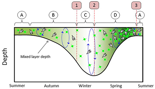
Figure 1. Stylized annual plankton cycle, beginning on left in midsummer and ending in early summer. Thick black line = mixed-layer depth (MLD). Green phytoplankton cells and green shading represent phytoplankton concentration. Gray ciliates stand for all phytoplankton predators. Circled A = summer condition of near-equilibrium between phytoplankton division and loss rates. Circled B = depletion phase. Circled C = phase where division exceeds loss but MLD is still deepening, phytoplankton concentrations are stable or decreasing, and phytoplankton biomass integrated over MLD is increasing. Circled D = accumulation phase. Boxed 1 = winter transition. Boxed 2 = transition to increasing phytoplankton concentration. Boxed 3 = climax transition.

The above description of Figure 1 is a very simplistic depiction of the DRH and a far more thorough account can be found in Behrenfeld and Boss (2018). The relevant information here is that the DRH identifies key events and phases in bloom-forming phytoplankton annual cycles and these events helped guide the design of NAAMES. Specifically, the field campaigns were conducted in early winter (November-December), early spring (March-April), late spring (May-June), and early autumn (September) to target, respectively, the “winter transition” (Figure 1 first red line and red box “1”), early stages of the “accumulation phase” (Figure 1 circle “D”), the “climax transition” (Figure 1 third red line and red box “3”), and early stages of the “depletion phase” (Figure 1 circle “B”). Thus, NAAMES is a field campaign designed to test the DRH hypothesis and advance understanding of linkages between all stages of the plankton annual cycle, which distinguishes it from many predecessor studies focused solely on the final events of the spring bloom climax.

The NAAMES proposal was based heavily on satellite, autonomous sensor, and model results and our initial expectations were that (1) significant accumulations in phytoplankton biomass would not be observed when division rates were decelerating prior to the “winter transition,” (2) that similar rates of biomass accumulation would be observed following the “winter transition,” during the “accumulation phase,” and until just prior to the “climax transition,” and (3) that the “depletion phase” would be dominated by mixed layer loss rates exceeding phytoplankton division rates. Furthermore, we expected to see a tight coupling between phytoplankton division and loss rates during all four campaigns. With respect to community composition, we anticipated a dominance of small photosynthetic eukaryotes and prokaryotes during the “winter transition” campaign, dominance of diatoms during the “climax transition” campaign, and a potentially significant contribution of dinoflagellates during the “depletion phase” campaign. We also hoped to gain new insights from NAAMES on the role of plankton community compositional changes in governing bulk properties of the phytoplankton annual cycle. One of the exciting outcomes of NAAMES is that many of our original expectations proved to be incorrect, or at the least incomplete.

Biogenic Aerosols

The global ocean is an important source of aerosols to the remote marine atmosphere. These aerosols can be either directly emitted through sea spray (so-called primary marine aerosols) or generated in the atmosphere through photochemical oxidation and gas-to-particle conversion of ocean-derived trace gases (so-called secondary organic aerosols) (Gantt and Meskhidze, 2013). Primary marine aerosols are formed from wave breaking and bubble bursting processes that eject tiny droplets into the atmosphere. As submerged air bubbles rise through the ocean water column, they collect surface-active material (including particulate organic carbon, biological fragments, and dissolved organic matter) that partitions to the bubble interface (Lewis and Schwartz, 2004). At the ocean surface, an increasingly thinner film is produced as the bubble rises up against the sea surface microlayer, until finally the bubble bursts and sends a myriad of small, organically-enriched “film drops” into the air. Subsequently, the bubble cavity collapses and in this process forms a vertical jet of seawater that fragments into discrete “jet drops” (Lewis and Schwartz, 2004).

Since sea spray particles are driven by meteorology (wind speed) and particles generated from ocean-derived trace gases are driven by biological productivity, their contributions to aerosol particle concentrations have seasonal cycles that are expected to depend on these two factors. The basic features of these two competing seasonal cycles for aerosol production are illustrated in Figure 2. Starting in the summer on the left of Figure 2, elevated ocean productivity means that DMS emissions and hence sulfate particle contributions are high and then become reduced as productivity is reduced going into winter (Lana et al., 2011). Sulfate levels increase again in spring in a manner roughly following the increase in plankton populations shown in the DRH cycle of Figure 1, which peaks in late spring. Since organic components in sea spray and other aerosol particles are also produced by phytoplankton, their contributions to mass (and number) are expected to track sulfate, although the extremes may be dampened by the large reservoir of dissolved organic carbon that is ubiquitous in the ocean (Hansell et al., 2009). In contrast, sea spray is proportional to the square of the surface wind speed (typically measured at 10 m, or U10). This means that sea spray contributions to number concentration are lowest in summer when North Atlantic regional average wind speeds are near 7 m/s and highest in winter when wind speeds are nearly doubled (Young, 1999). Since wind-driven and convective mixing are strongest in winter, it is not surprising that the highest sea spray fluxes in Figure 2 coincide with the deep winter MLDs in Figure 1.

FIGURE 2

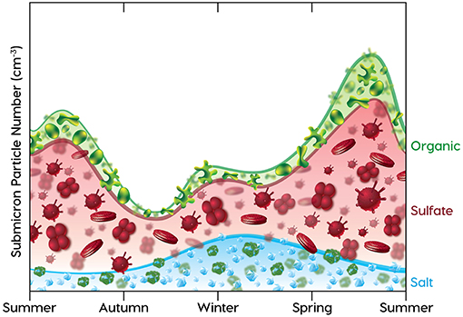
Figure 2. Stylized annual submicron aerosol number concentration cycle, beginning on left in midsummer and ending in early summer, showing contributions to number from sea spray salt (blue line), DMS-derived sulfate (red line), and ocean-derived organic (green line) components. The components are shown proportional to number, but should not be interpreted as externally-mixed particle populations. Blue line with NaCl cubes = ocean sea spray particles, scaled to interpolated monthly seasonal wind speed (U102) estimated from figure 1b of Young (1999). Red line with Prymnesiophyte (from NAAMES data) and Coccolithophore (from Bidle, 2015) images = sulfate-containing particle number concentrations scaled to monthly DMS emissions, estimated from figure 6 of Lana et al. (2011). Green line with organic component images (Hawkins and Russell, 2010) = organic-containing particle number concentrations, tracked to sulfate particle mass assuming similar seasonal productivity but 25% lower mass contribution. Relative contributions of each component to particle number concentrations are calculated from mass concentrations [for ranges reported in Table 1 of Sanchez et al. (2018)] by dividing by the cubes of modal diameters of 0.4 μm for sea spray particles, 0.2 μm for sulfate particles, and 0.3 μm for organic particles [using diameter ranges reported by Quinn et al. (2017) and Sanchez et al. (2018)].

Organic compounds play an important role in the cloud-forming potential of primary marine aerosol. While the typical concentrations of marine organics in seawater are dwarfed by the concentration of inorganic salts (i.e., on the order of a few tens of ppm organics vs. over thirty-thousand ppm salt), organics are a significant component of the primary submicron-sized aerosols that act as cloud condensation nuclei (CCN) due to their preferential partitioning to the bubble surface in the film drop formation mechanism (O'dowd et al., 2004; Facchini et al., 2008; Gantt and Meskhidze, 2013). These organics are consistent with known plankton exudate compounds (e.g., lipopolysaccharides and aliphatic chains with hydroxyl functional groups) that tend to form water-insoluble (and non-volatile) colloidal hydrogels (Verdugo et al., 2004; Facchini et al., 2008; Russell et al., 2010; Quinn et al., 2014). It also stands to reason that phytoplankton stress and mortality mechanisms also facilitate this process, especially during lytic virus infections that can lead to the massive releases of diverse cellular constituents and replicating colloidal virus particles (Bidle and Vardi, 2011). Indeed, viruses infecting coccolithophore populations in the North Atlantic have been detected within aerosols (Sharoni et al., 2015) and infection appears to stimulate the incorporation of free coccoliths into aerosols (Trainic et al., 2018). Each, in turn, may serve as particle nuclei that impact atmospheric compositional properties and dynamics of cloud formation.

Secondary marine aerosols are formed in the atmosphere through photochemical oxidation and subsequent gas-to-particle conversion of volatile sulfur-containing and organic trace gases, such as dimethylsulphide (DMS), isoprene, and other compounds (Saltzman et al., 1983; Shaw, 1983; Charlson et al., 1987; O'Dowd and de Leeuw, 2007; Quinn and Bates, 2011). This gas-to-particle conversion occurs through condensation onto pre-existing aerosols or through new particle formation (i.e., nucleation and subsequent growth) when ambient aerosol concentrations are low. Understanding the controls on marine aerosol and CCN budgets is important because they impact remote marine clouds and, hence, regional climate. Models suggest that marine clouds are particularly sensitive to CCN variability (Moore et al., 2013b) and satellite-based studies have shown periods of increased ocean biological productivity to double cloud droplet number and increase reflected solar radiation by 10 to 15 W/m² (Meskhidze and Nenes, 2006; McCoy et al., 2015). While an increase in ocean-derived biogenic aerosol is implied by these studies, a clear and direct linkage has yet to be established.

A challenge for NAAMES that was identified during the planning stage was how to distinguish the (expected) small fingerprint of ocean biology on atmospheric aerosols and clouds against a background of transported North American pollution. A surprising result from the field campaigns was that continental pollution only infrequently had a large influence on the marine boundary layer in the open ocean region of the NAAMES study. Aircraft vertical profiles did find pollution aloft in the free troposphere, but it was not clear that these transported emissions meaningfully impacted boundary layer CCN concentrations or cloud properties. Instead, the dominant seasonal driver of aerosol abundance appeared to be associated with local meteorology and effects of precipitation “cleaning” the atmosphere by removing aerosols to the ocean surface.

Scientific advances over past decades have dramatically expanded our conceptual model of the coupled ocean-atmosphere system. Major uncertainties remain, however, in quantifying the contribution of primary and secondary aerosols to the marine boundary layer CCN budget. The relative contribution of sea salt and organic aerosols to CCN have only recently become more fully understood (Sanchez et al., 2018), with the multiple NAAMES deployments uncovering the seasonal variation in each aerosol component (Figure 2). Linkages between observed atmospheric properties and variations in ocean ecosystems are not fully understood, with the atmospheric community realizing that reliance on chlorophyll-a concentration as a proxy for biological activity and emission of biogenic aerosol precursors is an oversimplification (Rinaldi et al., 2013). A key objective for NAAMES is to use a comprehensive set of ship and aircraft observations across seasons to constrain linkages between ocean ecosystem properties and biogenic aerosols, with an ultimate goal to improve predictions of marine aerosol-cloud-climate interactions from pre-industrial conditions (e.g., Carslaw et al., 2017) to those of a warmer future ocean.

NAAMES Experimental Design and Measurements

The western subarctic Atlantic (Figure 3) was chosen as the investigation site for NAAMES primarily because it (1) has been far less studied with respect to open ocean phytoplankton annual cycles than the eastern side of the subarctic basin, (2) experiences significant periods of very low atmospheric aerosol concentrations (thus increasing sensitivity to marine biogenic aerosols), (3) exhibits strong spatial and temporal variability in plankton biomass and composition (thus a large dynamic range for detecting ocean-aerosol-cloud effects), and (4) provided significant logistical advantages for the NAAMES research vessel and aircraft (e.g., shortened ship transit times from ports on the eastern margin of North America to open ocean conditions, multiple options for aircraft staging, minimal international logistics issues, etc.). Strong ocean physical features are also prominent in the western subarctic Atlantic, allowing sampling of cyclonic eddies, anticyclonic eddies, frontal zones, and non-eddy waters that are within relatively short ship transit distances. Furthermore, the NAAMES site connects long-term measurement records at multiple coastal atmospheric monitoring stations around the North Atlantic Ocean, including Mace Head, Ireland (https://www.macehead.org), Sable Island, Canada (http://afrg.peas.dal.ca/sableisland/index.php), the Azores (https://www.arm.gov/capabilities/observatories/ena), Cape Verde (https://www.ncas.ac.uk/en/cvao-home), and Barbados (Stevens et al., 2016). NAAMES C-130 transit flights between the NASA Wallops Flight Facility and St. John's, Canada, provided multiple opportunities for overflights of the Sable Island station where profiling measurements of atmospheric vertical structure were conducted over the island. Ship, aircraft, autonomous floats and drifters, and satellite observations were employed to address the science objectives of NAAMES. Ship measurements during all four of the ~26-day NAAMES cruises were conducted on the global-class research vessel (R/V) Atlantis. Ocean ecosystem properties measured on the ship focused on plankton stocks, biological rates (e.g., growth, predation), physiological stress, and community composition. A wide range of other relevant physical, chemical, and optical properties were concurrently measured with the ecosystem properties (Figure 4A). Ship-based aerosol related measurements targeted in-water aerosol precursors, sea-to-air gas flux measurements, and a detailed characterization of above-water aerosol concentrations, composition, and cloud condensation nuclei (CCN) (Figure 4B). Aircraft deployments were coordinated with the ship transect (Figure 3) and provided in situ aerosol and cloud measurements and remote sensing measurements of the ocean and atmosphere (Figure 4C). This coordinated effort was conducted to (1) broaden the spatial context of ship observations toward that of satellite remote sensing, (2) link ship-based near-surface aerosol properties to higher-altitude tropospheric aerosols and clouds, and (3) provide information on oceanic and atmospheric properties around ship sampling stations prior to arrival at and following departure from a given station. Autonomous drifters were deployed at ship stations during each NAAMES campaign to allow water tracking during station occupation and to provide a Lagrangian “bread crumb trail” for later revisits by the aircraft. In addition, 19 BioARGO floats were deployed at selected ship stations during the first three NAAMES campaigns. Each float had, at a minimum, an instrument payload measuring conductivity, temperature, pressure, chlorophyll fluorescence, oxygen, and particulate backscattering. A primary objective of the float deployments was to mechanistically link the four field campaigns within the context of the full annual plankton cycle. Floats deployed during a given campaign also provided station targets for subsequent campaigns. Finally, satellite data of winds, clouds, sea surface height, sea surface temperature (SST), and ocean color were used for ship station and flight planning and, as analyses continue, these data will provide context on year-to-year variability to assess the representativeness of the NAAMES campaigns and allow interpretation of field results in the context of the full subarctic Atlantic basin.

FIGURE 3

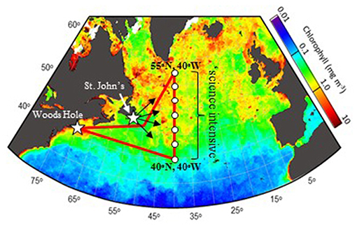
Figure 3. NAAMES study region and nominal campaign plan. Red line = ship track. White circles = ship stations. White stars = Woods Hole, MA, USA and St. John's, Newfoundland, Canada. Black arrows = aircraft flights heading toward “science intensive” region bound between 40°N and 55°N along 40°W longitude. Background color shows satellite-based surface chlorophyll concentrations for June 2002, exemplifying a typical bloom.

FIGURE 4

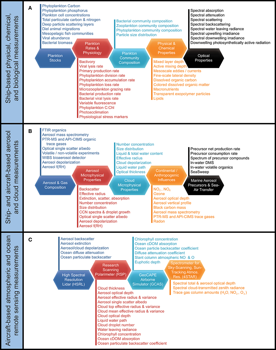
Figure 4. NAAMES measurements. (A) Ship-based measurements targeting (dark blue hexagon) plankton stocks, (red hexagon) plankton rates and physiology, (light blue hexagon) plankton community composition, (orange hexagon) physical and chemical properties, and (black hexagon) optical properties. (B) Ship- and aircraft-based measurements targeting (dark blue hexagon) aerosol and gas composition, (red hexagon) aerosol microphysical properties, (light blue hexagon) cloud microphysical properties, (orange hexagon) continental and anthropogenic influences, and (black hexagon) marine aerosol precursors and genesis. (C) Aircraft-based atmospheric and ocean remote sensing measurements from (dark blue hexagon) HSRL, (red hexagon) RSP, (light blue hexagon) GCAS, and (orange hexagon) 4STAR.

The nominal ship cruise plan (Figure 3) for each campaign entailed an initial transit from Woods Hole, Massachusetts (USA) to 40° W, during which measurements were limited to those that could be conducted underway (i.e., no station data). The primary “science-intensive” transect (~14 days) of the nominal cruise plan extended between ~40° N and ~55° N latitude along the 40° W longitude line (Figure 3), which encompasses three of the regional satellite data bins analyzed in Behrenfeld (2010) and Behrenfeld et al. (2013). Multiple sampling stations were occupied along the “science intensive” transect and were numbered sequentially for each campaign (e.g., Station 4 during the third NAAMES campaign was not geographically in the same location as Station 4 during the fourth NAAMES campaign). A key attribute of the latitudinal span of the science-intensive transect is that it temporally compresses developmental stages of the phytoplankton annual cycle. Thus, the NAAMES design traded space for time by using latitudinal gradients in seasonal phenology to sample a broader range of conditions during the 2-week intensive sampling period. Specifically, the “winter transition,” “climax transition,” “accumulation phase,” and “declining phase” all begin earlier at lower, relative to higher, latitudes of the subarctic Atlantic (Siegel et al., 2002; Behrenfeld, 2010; Behrenfeld et al., 2013). What this means is that within the limited 14-day science-intensive transect, NAAMES can sample a range of stages in the plankton annual cycle that might otherwise take months to unfold at a single location. For example, pre-climax, climax, and post-climax populations were all encountered during the single “climax transition” NAAMES campaign. An additional advantage of the latitudinal range encompassed by the science-intensive transect is that it helped ensure that the primary targeted event for a given campaign was actually encountered despite interannual variability in the timing of the event. For example, if the “climax transition” campaign was scheduled for a year where bloom development was anomalously late, then a climax community would be encountered at a lower latitude than during a year when bloom development was earlier.

The NAAMES C-130 aircraft provided a complementary perspective on regional variability in ocean and atmosphere properties around the R/V Atlantis. The aircraft was based at St. John's International Airport in Newfoundland, Canada, which is at the easternmost point of North America and thus minimized flight distances to the ship. Multiple 10-h science flights typically targeting ship stations were conducted during the first three NAAMES campaigns. A standard flight pattern was followed to provide reasonable spatial correspondence between low-altitude in situ aerosol-cloud sampling and high-altitude remote sensing of the ocean surface and overlying aerosols and clouds. The standard flight plan is shown in Figure 5 and consisted of a “Z-pattern” of ~150-km-long stacked high- and low-altitude legs with midpoints spaced approximately 50 km on either side of the R/V Atlantis (the ship position is at the midpoint of the Z diagonal). The outermost portions of the “Z-pattern” each included a descending spiral where the aircraft transitioned from the high-altitude leg to the low-altitude leg. These two spirals provided important constraints on the vertical structure of the atmosphere. After completing the first set of high- and low-altitude “Z-pattern” legs, the aircraft returned to the ship at low altitude (important for ship and aircraft instrument intercomparisons). Upon reaching the ship, the aircraft completed a series of vertically stacked legs of ~40–80 km length designed to capture below-, in-, and above-cloud aerosol and droplet microphysical and chemical properties. This “cloud module” (Figure 5) consisted of six flight legs: (1) the lowest permissible flight altitude (~90 m altitude), (2) a clear-air, below-cloud leg, (3) an in-cloud leg near cloud base, (4) a clear-air, above-cloud leg, (5) an in-cloud leg near cloud top, and (6) a high-altitude remote sensing leg at ~6 km altitude. After completing the high-altitude portion of the “cloud module,” the aircraft continued along the diagonal of the “Z-pattern” to carry out the second pair of stacked high- and low-altitude legs. The spatial orientation of the “Z-pattern” and “cloud module” legs were chosen to coincide with the median solar azimuthal angle. Orienting the aircraft close to the principal solar plane was important for some of the airborne passive remote sensor retrievals. This was particularly true for the “winter transition” NAAMES campaign (November 2015) because solar elevations were close to minimum requirements for these retrievals.

FIGURE 5

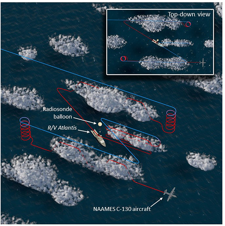
Figure 5. Nominal NAAMES aircraft sampling pattern. High-altitude, remote sensing legs (~6 km) are colored blue, while lower-level legs sampling below, in, and above clouds are colored red. The R/V Atlantis is shown at the center of the pattern near the left-most edge of the cloud module, while a radiosonde balloon is visible in the scene. The inset, top-down view shows the similarity of the flight pattern to the letter “Z,” when viewed from above.

The standard flight pattern described above accomplished a number of NAAMES ocean and atmosphere observational objectives. The length scale of the “Z-pattern” was such that the remote sensing legs transected prominent ocean eddy features. The “Z-pattern” also provided regional context for the ship-based aerosol measurements to assess variability over fine spatial scales. The combined high- and low-altitude legs offered an unparalleled data set for advancing new active and passive remote sensing retrieval algorithms for aerosols and clouds (e.g., Alexandrov et al., 2018; Sinclair et al., in review). The additional “cloud module” provided important data on marine boundary layer aerosol and cloud properties suitable for process-based studies combining models and observations. More than 20 “cloud modules” were completed during the first 3 NAAMES deployments, which will be described in a future publication.

In addition to the science benefits noted above, standardizing the flight pattern also greatly simplified the advanced planning process and reservation of air space for campaign flights. Large rectangular and stationary air space reservations were made encompassing the projected and completed NAAMES cruise track. Air space reservations were also designed to allow targeted overflights of cloud breaks in the quickly evolving cloud deck encountered during NAAMES, thus improving surface ocean observations. A typical 10-h flight consisted of an ~2 h outbound transit, ~2 h inbound transit, and, between these two transits, an ~4 h period to complete the standard pattern (Figure 5). Two additional hours of flexible flight time were thus available for condition-specific observations, such as high-altitude remote sensing surveys along the ship track, additional cloud modules targeting an atmospheric feature of interest, low-altitude in situ surveys of marine boundary layer aerosols and clouds, and Lagrangian transects of air masses that trajectory modeling indicated would impact the ship over subsequent hours to days.

Atmosphere and ocean modeling and data synthesis components are incorporated in NAAMES to (1) provide a historical background and inform pre-mission deployment planning, (2) contribute a quantitative, regional framework for interpreting field and satellite data, and (3) translate the conceptual and mechanistic findings from NAAMES into the Earth system models used to study large-scale environmental and climate change (Bonan and Doney, 2018). The primary tools for ocean modeling include physical-biogeochemical hindcast and high-resolution mesoscale simulations with the ocean component of the Community Earth System Model (CESM) (Behrenfeld et al., 2013; Moore et al., 2013a; Harrison et al., 2018). Ongoing studies are being conducted to evaluate and improve model skill using detailed comparisons against NAAMES field data, characterize the seasonal phenology and underlying dynamical balance governing phytoplankton populations of the subarctic Atlantic, and quantify biophysical mesoscale variability using geostatistical techniques applied to both eddy-resolving simulations and remote sensing data.

The main tools and data sets for tropospheric aerosol and transport modeling included the NASA Goddard Earth Observing System version 5 (GEOS-5; Rienecker et al., 2008; Molod et al., 2012) near real-time 10-day weather and aerosol forecasts (https://gmao.gsfc.nasa.gov/forecasts/), the Modern-Era Retrospective analysis for Research and Applications, version 2 (MERRA-2; Gelaro, 2017), the GEOS-Chem chemical transport model (Bey et al., 2001; Park et al., 2004), and the FLEXible PARTicle dispersion model (FLEXPART, Stohl et al., 1998). The GEOS-5 forecasts were used daily to generate animations of meteorological variables, aerosols, and pollution tracers for the western North Atlantic, as well as curtains along the planned cruise and flight tracks. These products provided critical guidance to flight planning and useful information to the NAAMES science team during the campaigns. The MERRA-2 reanalysis includes assimilation of space-based observations of aerosols (Randles et al., 2017) and is incorporated into the NAAMES data archive for comparison analysis. The GEOS-Chem model hindcast simulations were driven by the MERRA-2 meteorological reanalysis and were tested and evaluated against the NAAMES field observations, as well as other ground, in-situ, and satellite measurements. Hindcast simulations were used to examine the major transport pathways for North American pollution outflow to the study region and to quantify the terrestrial and marine sources of aerosols during NAAMES. FLEXPART simulations were conducted to estimate transport pathways and origins of air masses encountered by the ship and aircraft during NAAMES. The trajectory products are included in the NAAMES data archive (see below).

Campaign #1: Winter Transition

The first NAAMES campaign was conducted between November 5 and December 2, 2015. The ship transit began from Woods Hole, MA, headed to the planned northernmost latitude and then continued south roughly along 40°W longitude before returning to Woods Hole (Figure 6A). The science-intensive segment of the cruise spanned from ~54°N to ~40°N and included seven primary stations (labeled Station S1–S7) with Niskin bottle sampling of the water column (Table 1). Three of these stations were located inside anticyclonic eddies, two were in cyclonic eddies, and two were outside of eddies (Figure 6A; Table 1). Satellite ocean color coverage of the region was poor during NAAMES 1, but data that were available indicated low chlorophyll concentrations (Figure 6B). Surface drifters were deployed at each station and five BioARGO floats were deployed, with two floats at Station S2 and one float each at Stations S1, S3, and S4 (Figure 6C; Table 1). Sea Sweep, a sea spray aerosol generator (Bates et al., 2012), was deployed seven times during the cruise, with three deployments at Station S2, one deployment each at Stations S4 and S6, and 2 deployments at Station S7. Five 10-h C-130 flights were executed during the campaign and provided measurements spanning the full domain of the ship transit (Figure 6D; Table 2).

FIGURE 6

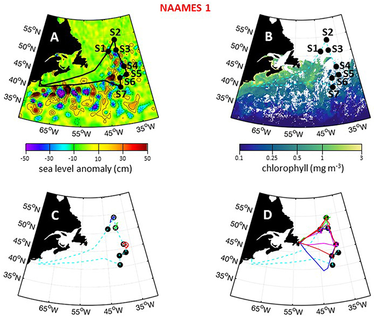
Figure 6. NAAMES 1 primary stations, autonomous floats, and flight tracks. (A) Black line = ship transit. Labeled black circles = primary sampling stations. Background color = sea surface height anomalies highlighting anticyclonic and cyclonic mesoscale eddies in red and blue/purple, respectively. (B) Climatological surface chlorophyll concentrations for the NAAMES 1 period from satellite ocean color measurements. (C) Float trajectories up to 30 days following the campaign. Star = float deployment site. (D) C-130 flight paths for the NAAMES 1 airborne campaign. Broken cyan line in (B–D) = ship track.

TABLE 1

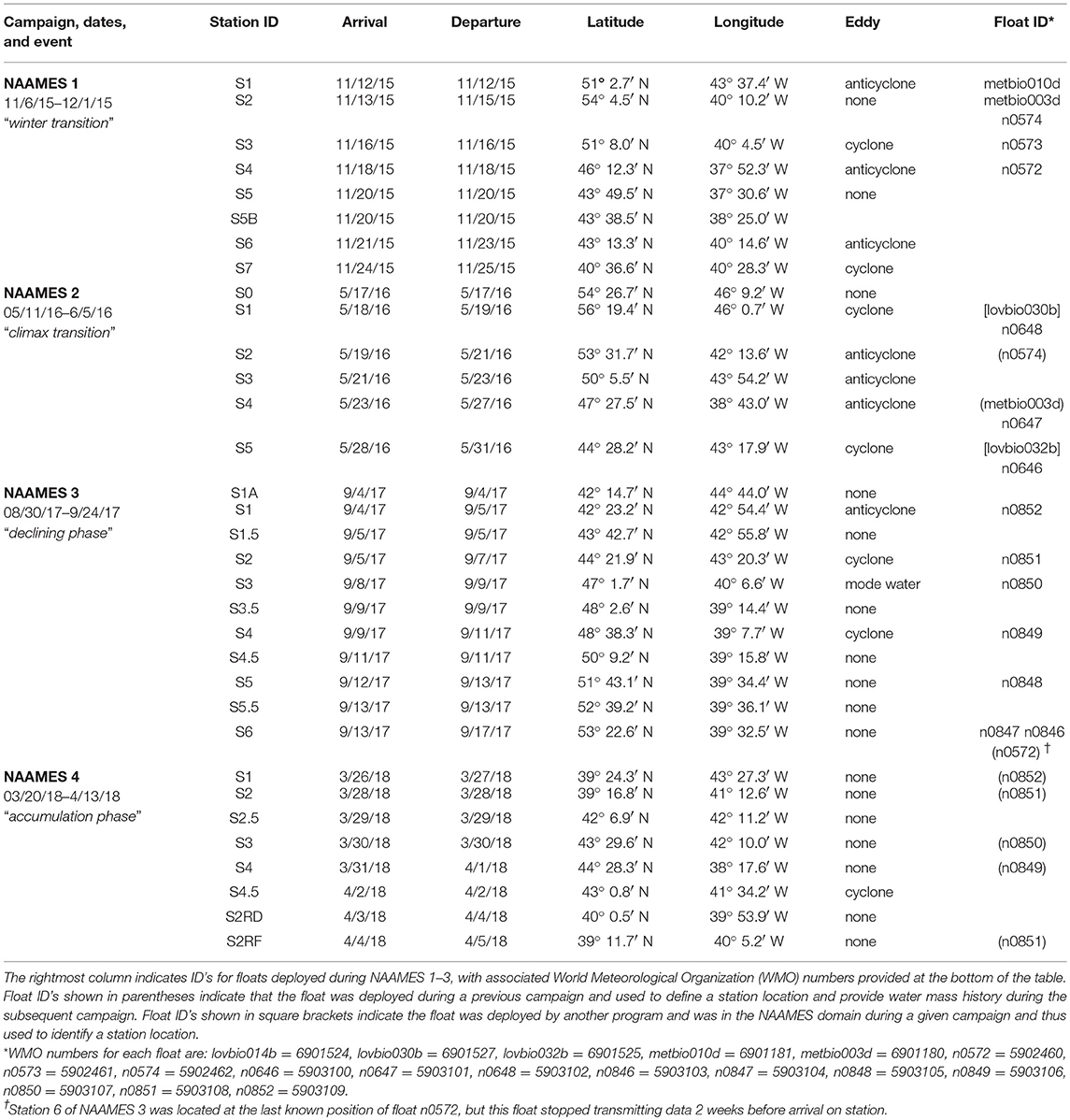
Table 1. Summary of NAAMES ship stations.

TABLE 2

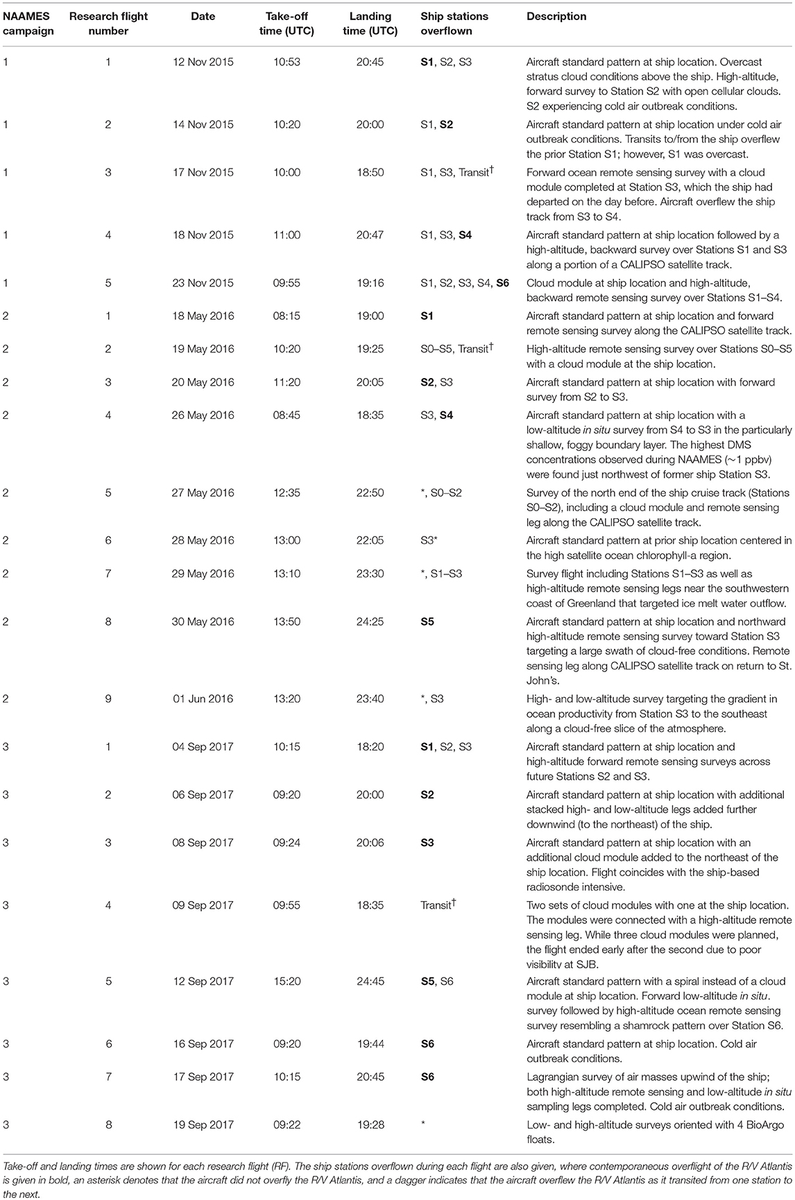
Table 2. Summary of NAAMES aircraft flights.

During NAAMES 1, SST was <10°C at the northernmost stations and >15°C at the southern stations (Figure 7A). High winds and sea states were frequently encountered during this campaign and on occasion prohibited overboard deployments. Mixed layer depths across the science-intensive segment of the cruise exceeded 100 m. Incident photosynthetically active radiation (PAR) was low and frequent cloud cover often compromised airborne observations of the sea surface. During the outbound and return transits, chlorophyll concentrations were elevated (>1 mg m⁻³) on the continental shelf (Figure 7A). In the open ocean, chlorophyll levels were modest (~0.5 to 1 mg m⁻³) at the northern stations and low (<0.2 mg m⁻³) at stations south of 45°N (Figure 7A). Phytoplankton cell concentrations were generally low during NAAMES 1 compared to the other NAAMES campaigns, but these communities were taxonomically diverse, with observations of large pennate diatoms, centric diatoms characteristic of subpolar waters (e.g., Corethron), prymnesiophytes, cryptophytes, silicoflagellates, picoeukaryotes, and prokaryotes, including even Prochlorococcus at one of the northernmost stations. Dawn values of normalized variable fluorescence (F_v/F_m) were elevated (~0.5) at all locations, suggesting low levels of physiological stress.

FIGURE 7

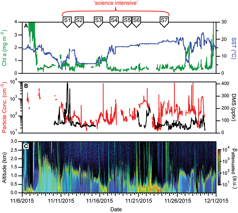
Figure 7. Ocean and atmosphere properties as a function of campaign date during NAAMES 1. (A) Surface chlorophyll concentration (green line) and sea surface temperature (SST; blue line) as a function of hours along ship transit. (B) Particle number concentration (red line) and dimethylsulfide gas mixing ratio (black line) along the ship transit. (C) Attenuated backscatter curtain in arbitrary units as detected by the ship-based ceilometer along the ship transit. The record begins on 11/6/2015 at 40° 27′ N, 70° 2′ W on the outbound transit and ends on 12/1/2015 at 41° 30′ N, 70° 41′ W on the return transit. Red bracket = “science intensive” segment of transit. Labeled symbols at top of panel indicate ship location at the beginning of each primary station (S1–S7).

For much of the cruise and flights, low aerosol and CCN concentrations of a few tens of particles per cm³ were observed in the marine boundary layer, which was often strongly influenced by polar air advected down the Labrador Strait to the NAAMES study region (Figure 7B). Anecdotally, scientists on the R/V Atlantis reported being unable to see the familiar plume of steam wafting up from their morning cup of coffee, as there were insufficient ambient particles on which water vapor could condense. DMS concentrations in the marine boundary layer were low (~30–50 pptv, Figure 7B). Clouds encountered during NAAMES 1 appeared to consist of supercooled droplets, which were observed to cause significant icing on aircraft inlets and probes as the aircraft ascended and descended through the cloud tops. Icing of the aerosol isokinetic inlet during a cloud-top leg in the first research flight was so severe that the order of the above cloud and cloud top legs were reversed for the cloud modules in all subsequent flights to avoid icing to the greatest extent possible. Conditions over the R/V Atlantis were commonly cloudy with solid stratiform clouds at Station 1 (11/12–11/13) transitioning to open cell cloud structures in the following days (Figure 7C). The period from 11/19 to 11/25 experienced shallow boundary layers and frequent precipitation (Figure 7C).

Campaign #2: Climax Transition

The second NAAMES campaign was conducted between May 11 and June 5, 2016. As with NAAMES 1, the ship transit during NAAMES 2 began from Woods Hole, MA, headed to the planned northernmost latitude and then continued south roughly along 40°W longitude before returning to Woods Hole (Figure 8A). The science-intensive segment of this cruise spanned from ~56°N to ~44°N and included five primary stations (labeled S1–S5) and one initial “test station” (labeled S0) (Table 1). Two stations were located in cyclonic eddies, three stations in anticyclonic eddies, and one station outside of eddies (Figure 8A; Table 1). Relative to NAAMES 1, satellite ocean color coverage during NAAMES 2 was improved and indicated an increasing gradient in surface chlorophyll concentration with latitude, often exceeding 1 mg m⁻³ between Stations S1 and S4 (Figure 8B). Surface drifters were deployed at each station, but manufacturer defects in the batteries caused half of these drifters to never turn on and the other half to have lifetimes of only a few weeks rather than the typical lifetime of a few years. Three BioARGO floats were deployed, with one float each at Stations S1, S4, and S5 (Figure 8C; Table 1). Six additional ARGO floats were deployed during NAAMES 2, four with only a conductivity-temperature-pressure (CTD) sensor and two with CTD and oxygen sensors. Sea Sweep was deployed eight times during the cruise, with at least one deployment at each primary station. Nine 10-h C-130 flights were executed during the campaign and provided measurements spanning the full domain of the ship transit, as well as off the southwest coast of Greenland (Figure 8D; Table 2).

FIGURE 8

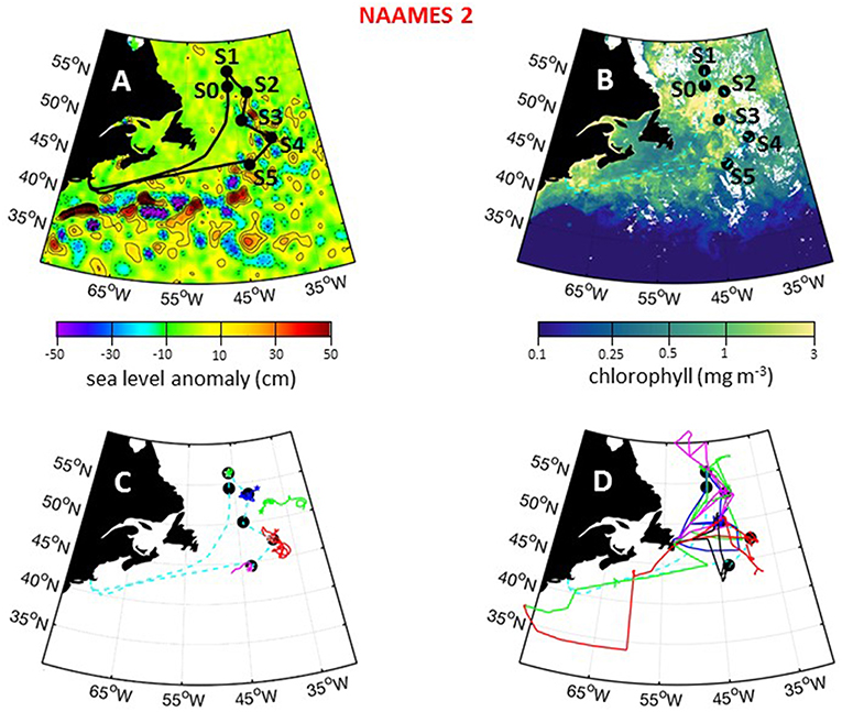
Figure 8. NAAMES 2 primary stations, autonomous floats, and flight tracks. (A) Black line = ship transit. Labeled black circles = primary sampling stations. Background color = sea surface height anomalies highlighting anticyclonic and cyclonic mesoscale eddies in red and blue/purple, respectively. (B) Climatological surface chlorophyll concentrations for the NAAMES 2 period from satellite ocean color measurements. (C) Thirty-day trajectories for floats deployed during NAAMES 2 and 130 days for floats deployed before NAAMES 2. Star = float deployment site. (D) C-130 flight paths for the NAAMES 2 airborne campaign. Broken cyan line in (B–D) = ship track.

During NAAMES 2, sea state and wind conditions were generally favorable (note exceptions below) and rarely prohibited overboard deployments. Incident PAR was elevated relative to NAAMES 1, but varied significantly from day-to-day due to frequent overcast skies that once again made airborne observations of the sea surface “opportunistic.” Mixed layer depths at all stations generally ranged from 20 to 60 m (again, note exceptions below). A sharp transition in ocean conditions was encountered along the science-intensive segment at ~50°N (Figure 9A). North of this transition, SST was generally <10°C and chlorophyll concentrations ranged from ~2 mg m⁻³ to >10 mg m⁻³ (Figure 9A). At the transition, SST was ~15°C and chlorophyll concentration dropped precipitously to <2 mg m⁻³. At all open ocean locations, phytoplankton biomass during NAAMES 2 was dominated by cells of <20 μm diameter. Dawn F_v/F_m values of ~0.5 were again observed across most of the ship transit, except between stations S4 and S5 where values decreased slightly to ~0.4.

FIGURE 9

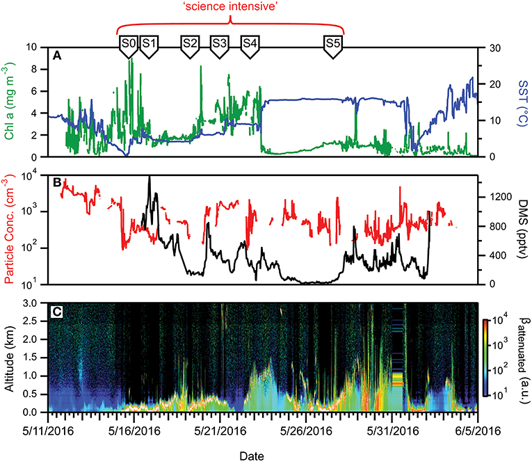
Figure 9. Ocean and atmosphere properties as a function of campaign date during NAAMES 2. (A) Surface chlorophyll concentration (green line) and sea surface temperature (SST; blue line) as a function of hours along ship transit. (B) Particle number concentration (red line) and dimethylsulfide gas mixing ratio (black line) along the ship transit. (C) Attenuated backscatter curtain in arbitrary units as detected by the ship-based ceilometer along the ship transit. The record begins on 5/11/2016 at 40° 31′ N, 70° 17′ W on the outbound transit and ends on 6/5/2016 at 41° 29′ N, 70° 41′ W on the return transit. Red bracket = “science intensive” segment of transit. Labeled symbols at top of panel indicate ship location at the beginning of each primary station (S0–S5).

Aerosol and CCN concentrations observed during NAAMES 2 were substantially higher than during NAAMES 1. Typical surface aerosol concentrations were hundreds of particles per cm³ (Figure 9B). DMS concentrations measured by the aircraft were also elevated relative to November, with a median concentration near 75 pptv and similar to DMS values measured on the ship (Figure 9B). During the 26 May 2016 research flight, DMS concentrations in an especially shallow and foggy boundary layer near Station S3 exceeded 1,000 pptv and there was also a detectable presence of dimethylsulfoxide (DMSO). The high concentrations of DMS underscore the potential importance of both ocean emissions and boundary layer dynamics in driving atmospheric concentrations of trace gas species. The atmospheric boundary layer over the R/V Atlantis was shallower during the beginning portion of the May cruise than typically observed during the November cruise (Figures 7C, 9C). Overcast cloud conditions were also frequent.

Two unique opportunities were presented during NAAMES 2. The first of these occurred during the transit between Stations S3 and S4 when a strong weather system moved into the area and deepened regional mixed layers. Upon arrival at Station S4, the water column was uniform in physical and biological properties to a depth of ~250 m. The mixed layer subsequently shoaled rapidly to <20 m (Graff and Behrenfeld, 2018). This event provided the rare opportunity to witness the “recovery” of a plankton community following an acute “disturbance” (Behrenfeld and Boss, 2018). Specifically, the deep mixing event caused a previously shallow plankton community to be diluted into a large volume of water, which is anticipated to strongly decouple phytoplankton division and loss rates due to reduced phytoplankton-zooplankton encounter rates (Behrenfeld and Boss, 2018). Subsequent shoaling of the mixed layer was expected to result in an immediate increase in phytoplankton concentration followed by a grazer response to enhanced food supply. In other words, a “recoupling” of division and loss rates. To follow this ecological event, occupation of Station S4 was prolonged to 4 days. This extended Station S4 also allowed the export of dissolved and suspended matter into the mesopelagic zone from convective mixing to be documented. Physical, chemical, ecological, and aerosol changes observed at Station S4 are topics for other manuscripts. Graff and Behrenfeld (2018) describe the physiological response of the phytoplankton community during the Station S4 occupation.

The second unique opportunity during NAAMES 2 occurred at Station S5 when the center of a strong low-pressure (993 mb) storm passed directly over the ship's location (Figure 10). While severe weather conditions during the storm prevented any overboard deployments and even access to the weather decks, the event did provide a rare opportunity to measure sea-to-air aerosol gas fluxes under extreme conditions with high wind speeds and large waves. A description of results from these measurements is anticipated in a future manuscript.

FIGURE 10

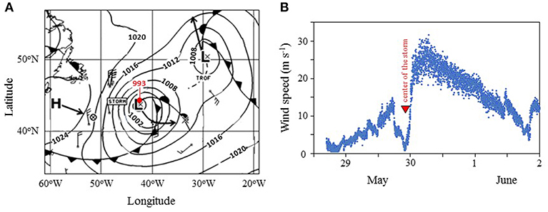
Figure 10. Meteorological conditions during occupation of Station S5 of NAAMES 2. (A) Atlantic Surface Analysis Map from 5/30/2016 at 00 UTC. Contours show surface pressure (mb). Red dot indicates location of R/V Atlantis (surface pressure = 993 mb). L = low pressure system, with arrow showing forecasted trajectory. H = high pressure system, with arrow showing forecasted trajectory. Lines with solid triangles = cold front. Lines with solid semicircles = warm front. Data from the National Oceanographic and Atmospheric Administration (NOAA). (B) Wind speed temporal record measured on the ship during occupation of Station S5 of NAAMES 2.

Campaign #3: Declining Phase

The third NAAMES campaign was conducted between August 30 and September 24, 2017. The ship transit began from Woods Hole, MA, headed to the planned southernmost latitude and then continued north roughly along 40°W longitude before returning to Woods Hole (Figure 11A). The science-intensive segment of this cruise spanned from ~42 to ~53°N and included six primary stations (S1 to S6) and five secondary stations of brief occupation (S1A, S1.5, S3.5, S4.5, S5.5) (Table 1). Two stations were located inside anticyclonic eddies, with one of these in an intrathermocline or “mode-water type” anticyclone (Table 1). Two other stations were located in cyclonic eddies and two stations were outside of eddies (Figure 11A; Table 1). Satellite ocean color coverage during NAAMES 3 was the best of all campaigns and indicated low surface chlorophyll concentrations from Stations S1A to S4 and higher concentrations at Stations S5 and S6 (Figure 11B). Surface drifters were deployed at each station and seven BioARGO floats were deployed, with one float each at Stations S1–S5 and two floats at Station S6 (Figure 11C; Table 1). Sea Sweep was deployed eight times during the cruise, with two deployments at Stations S1 and S6 and one deployment each at Stations S2–S5. Eight, 10-h C-130 flights were executed during the campaign and provided excellent coverage of the ship transit (Figure 11D; Table 2). A set of microlayer samples were collected from all stations during NAAMES 3. During NAAMES 3, SST was generally warmer than the two previous campaigns and ranged between 10°C and 28°C (Figure 12A). A hurricane passing along the US eastern seaboard caused a slight delay in departure from Woods Hole. Over the course of the ship transit, multiple hurricanes developed in the tropical Atlantic, but fortunately most of these did not threaten NAAMES work and weather conditions were generally favorable for overboard deployments. The exception to this good fortune was hurricane José, which threatened to intercept the R/V Atlantis on its return transit from Station S6 to Woods Hole. Accordingly, occupation of Station S6 was slightly foreshortened to allow sufficient time to seek refuge in inland waters if the hurricane continued along its forecasted trajectory. In the end, the NAAMES cruise got lucky once more when hurricane José changed course to the south and only peripherally influenced sea states encountered by the ship on its transit home.

FIGURE 11

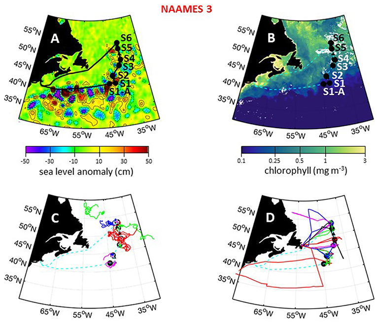
Figure 11. NAAMES 3 primary stations, autonomous floats, and flight tracks. (A) Black line = ship transit. Labeled black circles = primary sampling stations. Black triangles = in-between stations. Background color = sea surface height anomalies highlighting anticyclonic and cyclonic mesoscale eddies in red and blue/purple, respectively. (B) Climatological surface chlorophyll concentrations for the NAAMES 3 period from satellite ocean color measurements. (C) Thirty-day trajectories for floats deployed during NAAMES 3 and 130 days for floats deployed before NAAMES 3. Star = float deployment site. (D) C-130 flight paths for the NAAMES 3 airborne campaign. Background color = logarithm of MODIS surface chlorophyll concentration averaged over the campaign. Broken cyan line in (B–D) = ship track.

FIGURE 12

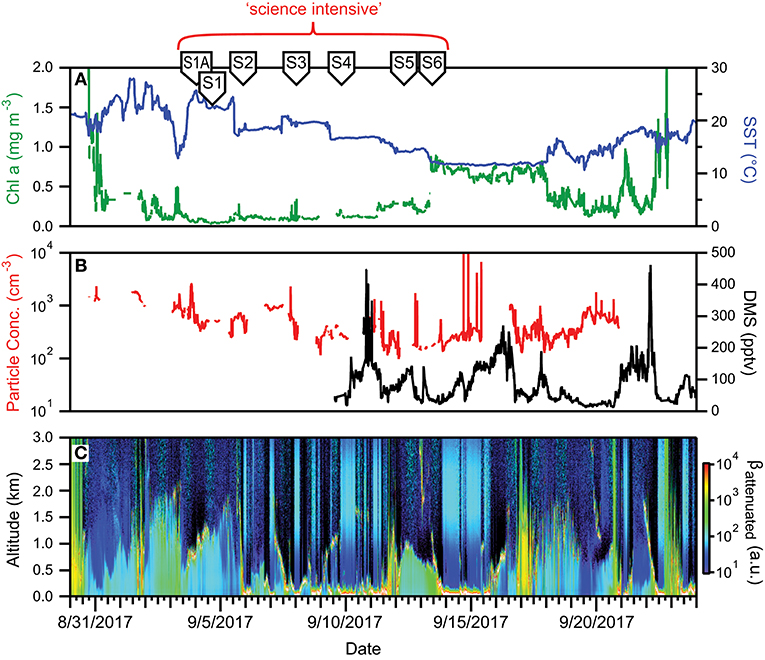
Figure 12. Ocean and atmosphere properties as a function of campaign date during NAAMES 3. (A) Surface chlorophyll concentration (green line) and sea surface temperature (SST; blue line) as a function of hours along ship transit. (B) Particle number concentration (red line) and dimethylsulfide gas mixing ratio (black line) along the ship transit. (C) Attenuated backscatter curtain in arbitrary units as detected by the ship-based ceilometer along the ship transit. The record begins on 8/30/2017 at 41° 9′ N, 70° 54′ W on the outbound transit and ends on 9/24/2017 at 41° 25′ N, 66° 59′ W on the return transit. Red bracket = “science intensive” segment of transit. Labeled symbols at top of panel indicate ship location at the beginning of each primary station (S1A–S6).

During the science-intensive segment of NAAMES 3, all stations had relatively shallow mixed layer depths that ranged from ~10 to ~40 m. Incident PAR was comparable to NAAMES 2, but less frequent cloud cover made NAAMES 3 the most successful campaign in terms of airborne observations of the sea surface. Chlorophyll-a concentrations were relatively low (<0.4 mg m⁻³) from Stations S1A to S5, but then exhibited a sharp increase to >0.7 mg m⁻³ between Stations S5 and S6 (Figure 12A). Moreover, Station S6 had the highest concentrations (by approximately an order of magnitude) of chlorophyll-b (~0.2 mg m⁻³) and chlorophyll-c (~0.25 mg m⁻³) of all four NAAMES campaigns. Between Stations S1A and S5, dawn values of F_v/F_m were ~0.45 to 0.5 and phytoplankton communities were dominated by Synechococcus, dinoflagellates, and other nano-eukaryotic cells, although a notable increase in phytodetritus was observed at some stations.

Surface aerosol concentrations measured on the ship ranged from ~1,000 cm⁻³ at the beginning of the “science intensive” transect to ~100 cm⁻³ as the ship moved northward toward S6 (Figure 12B). This transition reflected the influence of similar “cold air outbreak” conditions as in November, 2015. However, unlike NAAMES 1, aerosol and CCN concentrations never reached the ultra-low levels encountered during November, which may have been due to compensating sources of particles from either ocean surface emissions or from long-range transport. Boundary layer DMS concentrations were similar to those found in November (<100 pptv), albeit with some additional variability (Figure 12C). Cloud conditions during NAAMES 3 were most conducive for ocean remote sensing from the aircraft, as frequent breaks in the clouds were encountered (Figure 12C). Multiple periods with very shallow boundary layers (<0.5km) were also observed.

Encountering a declining phytoplankton community and both characterizing and quantifying the mortality and loss processes was of particular interest during NAAMES 3. It was spectacularly observed at Station S6, where dawn values of F_v/F_m were ~0.3 and lower than at any other station in all four NAAMES campaigns. These low F_v/F_m values suggested a phytoplankton population experiencing significant physiological stress. Routine measurements during NAAMES included diagnostic staining for reactive oxygen species (ROS) and live/dead cells (SYTOX positive) coupled with analytical flow cytometry and provided an in depth assessment of physiological stress across phytoplankton functional groups. Dinoflagellates were particularly abundant at Station S6 relative to other NAAMES stations. Satellite ocean color data suggested that Station S6 was at the southeastern end of a much larger phytoplankton die-off extending well into the Labrador Sea (Figure 13). Furthermore, prevailing winds were coming from the northwest, increasing the possibility that a strong signature of the declining population would be registered in biogenic aerosols. Because of these unique characteristics, Station S6 was occupied for the extended period of September 13–17th. Also during this time, ship-based radiosonde launch frequency was increased to every 2 h during the day and every 4 h at night in order to capture the temporal variation of the marine boundary layer temperature and humidity profiles. Back to back flights executed on September 16 and 17th included low-altitude in situ sampling surveys to the northwest of Station S6 to characterize biogenic aerosol above the plankton feature shown in Figure 13, as well as to sample air that would be advected to the ship over subsequent hours (Figure 14). The standard “Z-pattern” and “cloud module” were executed over the ship at Station S6 on September 16th. This unique Lagrangian sampling strategy will enable forthcoming process-based studies that examine the evolution of aerosols sampled by the aircraft upwind of the ship almost 24 h prior. In addition, the cold air outbreak case observed during September 16–17th, 2017, provides a contrast to that observed during November 12–14th, 2015, with an order of magnitude difference in boundary layer aerosol concentrations between the two cases.

FIGURE 13

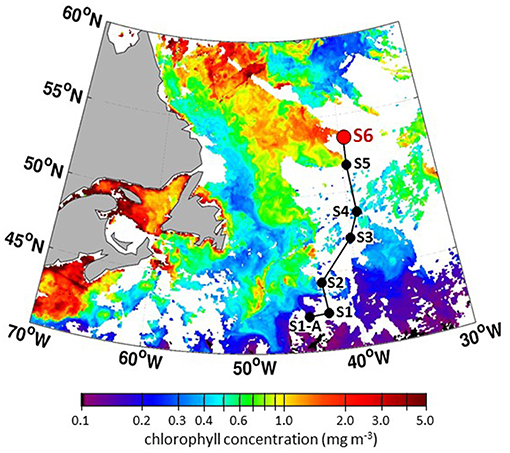
Figure 13. Composite MODIS chlorophyll concentrations for September 2–4, 2017 (dates with the best satellite coverage during NAAMES 3) showing stations along “science intensive” transit and massive feature extending from Station S6 (NAAMES 3) into the Labrador Sea.

FIGURE 14

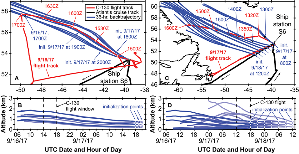
Figure 14. Summary of the Lagrangian sample experiment during NAAMES 3. Red lines in (a,b) denote the C-130 flight tracks from 16 to 17 September, while the black line denotes the R/V Atlantis cruise track in the vicinity of Station S6 (NAAMES 3). Blue lines in all panels show NOAA HYSPLIT air mass back trajectories initialized at the ship location (Station S6 on September 16th and at seven locations along the cruise track on September 17–18th). Red open circles show the UTC flight time for low-altitude sampling, while the filled blue circles on the HYPSLIT trajectories indicate the portion of the back trajectory that is spatially contemporaneous with the flight track. The vertical components of the back trajectories are shown in (b,d).

Campaign #4: Accumulation Phase

The fourth and final NAAMES campaign was conducted between March 20 and April 13, 2018. Prior to this campaign, a series of strong nor'easters passed through the western Atlantic. Fortuitously, ship scheduling of preceding R/V Atlantis cruises necessitated that NAAMES 4 departed from San Juan, Puerto Rico (rather than Woods Hole) and sailing conditions from San Juan to the first station at ~39°N, 43°W were pleasantly mild. The science-intensive segment of NAAMES 4 spanned from ~39°N to ~44.5°N (Table 1). Inclement weather prevented operations any further to the north. A total of 6 primary stations (S1–S4, S2RD, S2RF) and 1 secondary station (S2.1) were occupied during the cruise (Figure 15A), with each primary station determined by the location of operational floats deployed during previous cruises (Table 1). Regional surface chlorophyll concentrations were elevated over the continental shelf and highly variable around the NAAMES 4 stations (Figure 15B). At Station S2, the phytoplankton population was in an “accumulation” phase and chlorophyll concentrations were reasonably elevated. Between the occupation of Station S2 and S4, a storm passed through the Station S2 region and, based on available float data, significantly deepened the mixed layer. As with Station S4 of NAAMES 2, this event was expected to provide another opportunity for observing an ecological “disturbance.” Given the weather conditions to the north, it was therefore decided to re-occupy Station S2 after leaving Station S4. This re-occupation targeted the location of the Station S2 drifter (S2RD) and float (S2RF) (Figure 15A; Table 1). Unfortunately, the ship's hydroboom catastrophically failed at Station S4, so water column profiling with the CTD-rosette package was terminated and water sampling at stations S2RD and S2RF was primarily done using the flow-through system. Interestingly, our re-occupation of Station 2 did not bring us to the healthy blooming phytoplankton population we sampled during its original occupation, but rather revealed a phytoplankton community with many stressed or dead cells. Following Station S2RF, the ship transited to its home port at Woods Hole.

FIGURE 15

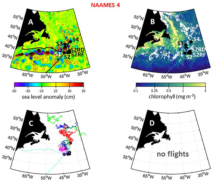
Figure 15. NAAMES 4 primary stations, autonomous floats, and flight tracks. (A) Black line = ship transit. Labeled black circles = primary sampling stations. Background color = sea surface height anomalies highlighting anticyclonic and cyclonic mesoscale eddies in red and blue/purple, respectively. (B) Climatological surface chlorophyll concentrations for the NAAMES 4 period from satellite ocean color measurements. (C) One hundred and thirty day trajectories for previously deployed floats that were still active during NAAMES 4. No new floats were deployed during NAAMES 4. Star = float deployment site. (D) No C-130 flights were conducted during NAAMES 4 due to mechanical issues with the aircraft. Broken cyan line in (B–D) = ship track.

For NAAMES 4, only Station S4.5 was in a cyclonic eddy (Table 1). This short station, however, only included sampling from the flow through system. Station S1 was on the periphery of an anticyclonic eddy and Station S2 was located between a cyclonic and anticyclonic eddy. Surface drifters were deployed at each station, but no BioARGO floats were released. The location and history of previously-deployed and active floats in the NAAMES domain during the cruise are shown in Figure 15C. Sea Sweep was deployed five times in the science-intensive region, with one deployment each at Stations S1, S2, S4, S2RD, and S2FR. No C-130 flights were conducted during NAAMES 4 due to mechanical failure of the aircraft upon arrival at the St. John's airport (Figure 15D).

Fast-moving weather systems persisted throughout NAAMES 4, which worsened sea states, slowed ship transit speeds, and challenged overboard deployments. Reasonably fair skies resulted in enhanced daily PAR flux on many days. Mixed layer depths in the science-intensive region ranged from 40 to 80 m, while SST ranged from 6 to ~18°C (Figure 16A). Perhaps one of the more notable attributes of NAAMES 4 compared to the three previous campaigns was the patchiness in chlorophyll concentration. Within the science-intensive region, chlorophyll levels were highly variable and ranged from <0.5 to >3.5 mg m⁻³, with rapid changes between low and high values often inversely related to changes in SST (Figure 16A). Ship-based measurements of aerosol concentrations were on the order of a few hundred particles per cm³, while DMS concentrations varied roughly between 100 and 400 pptv (Figure 16B). Boundary layer heights detected by the ceilometer on the ship varied from 0.5 to 2 km (Figure 16C).

FIGURE 16

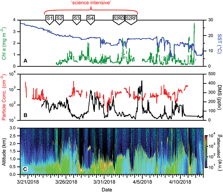
Figure 16. Ocean and atmosphere properties as a function of campaign date during NAAMES 4. (A) Surface chlorophyll concentration (green line) and sea surface temperature (SST; blue line) as a function of hours along ship transit. (B) Particle number concentration (red line) and dimethylsulfide gas mixing ratio (black line) along the ship transit. (C) Attenuated backscatter curtain in arbitrary units as detected by the ship-based ceilometer along the ship transit. The record begins on 3/20/2018 at 32° 32′ N, 51° 43′ W on the outbound transit and ends on 4/13/2018 at 41° 31′ N, 70° 40′ W on the return transit. Red bracket = “science intensive” segment of transit. Labeled symbols at top of panel indicate ship location at the beginning of each primary station (S1–S2RF).

Plankton Communities During NAAMES

During each NAAMES campaign, a wide variety of measurements were conducted to characterize plankton community composition. High-resolution taxonomic identifications of bacterial and phytoplankton cells were provided through genetic profiling. Additional information on community composition was provided by a BD Influx flow cytometer (size range = <1–64 μm), a Coulter Counter (size range = 2–50 μm), an Imaging Flowcytobot (IFCB) (size range = 5–150 μm), a FlowCam (size range = 30–300 μm), and an Underwater Video Profiler (UVP) (size range ~100–2,000 μm), along with High Performance Liquid Chromatography (HPLC) samples for phytoplankton pigments. This diversity of measurements over a broad size domain was intended not only to provide information on plankton diversity and abundance, but also to yield insights on ecological and environmental factors governing community structure over the annual cycle. It is anticipated that a number of manuscripts describing features of community composition during NAAMES will be shortly forthcoming. As a “first look,” a synoptic perspective of phytoplankton diversity across NAAMES 1, 2, and 3 is shown in Figure 17 (NAAMES 4 data were not yet available at the time of this writing). The figure ordinates phytoplankton rRNA genes by their abundance in samples, capturing about 1,000 taxa. Particularly striking is the strong correlation of axis 1 with latitude in samples from NAAMES 1 (November) and NAAMES 3 (September). A pronounced departure from this pattern is observed for NAAMES 2 (May), which largely ordinates along axis 2. Latitudinal variation in phytoplankton communities is well-recognized (Barton et al., 2010) but it emerges with unusual clarity here in the September and November data. The endmember of axis 2 is a sample cluster from Station S4 of NAAMES 2, which was the station noted above that captured initial blooming stages immediately following a deep-mixing “disturbance” event. The NAAMES 2 departure of bloom communities from the axis of latitudinal variation suggests that post-mixing blooms are communities at disequilibrium, but a more complex perspective might emerge when NAAMES 4 data are added to this analysis. The rich context of overlapping NAAMES data sets is supporting multivariate statistical approaches for studying factors controlling the composition of microbial plankton communities. For Figure 17, sequences were first parsed into a finely curated backbone tree representing phytoplankton taxonomic diversity. These data are currently being integrated with other phytoplankton diversity measurements collected during NAAMES to further resolve seasonal variation and bloom ontogeny in a richness of biological detail.

FIGURE 17

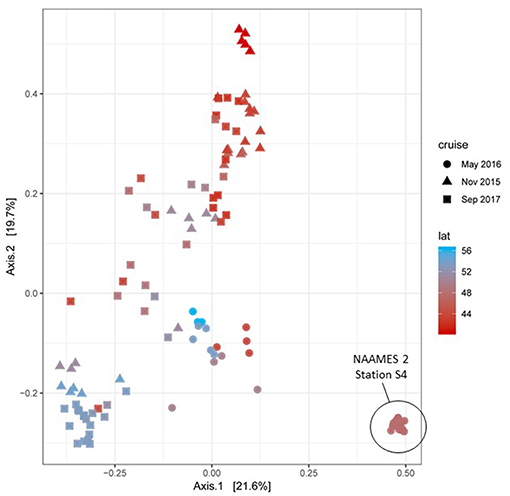
Figure 17. Principal Coordinates Analysis (PCoA) ordination of NAAMES 1, 2, and 3 phytoplankton communities based on 16S rRNA amplicon profiles. Sample datasets belonging to the upper 100m of the water column for each station were used to estimate Bray-Curtis distances between them. Datasets are colored in a red-blue gradient, with the northernmost station in navy blue and the southernmost station in red. Data point shapes identify the season when the sample was taken. Triangles = NAAMES 1 (November 2015). Circles = NAAMES 2 (May 2016). Squares = NAAMES 3 (September 2017). The variance explained by each principal coordinate is expressed in percentage and indicated on the axes.

NAAMES Data

Finalized versions of NAAMES field data, including documentation and metadata, are preserved and distributed through NASA's Distributed Active Archive Centers (DAACs). Due to the interdisciplinary diversity of the measurements collected by this project, they are divided between two different DAACs that specialize in serving different user communities (Table 3). NAAMES airborne and atmospheric measurements of trace gases, aerosol and cloud properties, and airborne-retrieved ocean properties are archived at the Atmospheric Science Data Center (ASDC; https://eosweb.larc.nasa.gov/). Ship-based and other in-water measurement data are archived in the SeaWiFS Bio-optical Archive and Storage System (SeaBASS; https://seabass.gsfc.nasa.gov/) maintained by the Ocean Biology DAAC (OB.DAAC). In addition, hyperspectral GCAS airborne data have been atmospherically corrected using approaches designed for variable platform altitudes, with iterations to account for non-zero water signal in the near-infrared wavelengths (Zhang et al., 2017, 2018). Surface spectral remote sensing reflectance from GCAS (Hierarchical Data Format-4) are available through the OB.DAAC. Currently, the transfer of data products to the ASDC is ongoing and its DOI has been reserved. In the interim, those data are available through the NASA Airborne Science Data for Atmospheric Science (ASD-AC; https://www-air.larc.nasa.gov/missions/naames/index.html). All project data are organized into standardized file formats approved by NASA Earthdata and each campaign's files are publicly released as soon as possible within a year of measurement collection. Data can be obtained through multiple methods, including entering the relevant DOI into a search engine (e.g., https://dx.doi.org) or using online tools available on the DAAC websites. SeaBASS has not historically supported distribution of plankton images, thus IFCB and UVP images and their retrieved properties (i.e., size parameters and other features derived from image analysis) have been uploaded on ECOTAXA, a web-based application that allows for the curation and annotation of images (http://ecotaxa.obs-vlfr.fr/prj/). Data from each cruise were saved as a separate project, with open access to all validated images.

TABLE 3

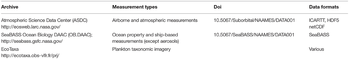
Table 3. Summary of NAAMES data access.

The NAAMES Legacy

NAAMES was based on two fundamental philosophies. First, understanding major events in plankton ecology, such as blooms, requires an evaluation of processes occurring over the full annual cycle. This philosophy stands apart from many earlier investigations where observations have often been constrained in time around a particular event. One benefit of the NAAMES approach is that it forces a broader view of ocean ecosystem functioning, where proposed mechanisms explaining one event must also be consistent with processes governing other periods of the annual cycle. The second philosophy of NAAMES was that a major advance in understanding of the coupled ocean biology and atmosphere system requires a balanced complement of integrated oceanic and atmospheric investigators sharing a common interdisciplinary research objective. This diversity of research backgrounds was fully achieved within the NAAMES science team (Table 4) and a clear cross-fertilization of data and ideas between investigators is emerging from the project.

TABLE 4

Table 4. The NAAMES team.

The NAAMES observational data set spans from details of plankton community structure and biological rates, to carbon cycling by the microbial loop, to in-water aerosol precursor concentrations and production/consumption rates, to processes regulating aerosol genesis, and the characterization of atmospheric aerosols and their links to cloud properties. At the time of this writing, only a few months had passed since the final NAAMES campaign. Nevertheless, new insights encompassed under NAAMES have been published regarding plankton annual cycles (Behrenfeld et al., 2016; Balaguru et al., 2018; Behrenfeld and Boss, 2018), phytoplankton physiology (Graff and Behrenfeld, 2018), mesoscale biology (Gaube et al., 2018; Glover et al., 2018), aerosols and cloud condensation nuclei (Quinn et al., 2017; Sanchez et al., 2018), and the biogeochemical pathways of aerosol precursor formation (Sun et al., 2016). Additional NAAMES publications have addressed improved measurement methodologies (Jones et al., 2017; Boss et al., 2018; Crosbie et al., 2018), new remote sensing algorithms (Zhang et al., 2017, 2018; Alexandrov et al., 2018; Sinclair et al., in review), and advances in satellite lidar ocean remote sensing (Behrenfeld et al., 2017; Hostetler et al., 2018). These successes are only the beginning of many additional publications we anticipate in coming years from the rich NAAMES data set that will support, as well as challenge, many ideas held on the ocean-atmosphere system before the NAAMES study was conducted.

Author Contributions

MB and RM led the writing of this manuscript. NAAMES leadership and manuscript figures, data, text, and comments were provided by CH, JG, PG, LR, GC, SD, SG, HL, CP, LB, NB, CD-M, TW, TSB, TGB, KB, EB, SB, BC, CC, KH, EH, CH, LK-B, MK, SM-D, FM, PQ, AS, BA, JC, EC, RF, JH, YH, SJ, JR, ES, MS, DS, AW, and LZ.

Conflict of Interest Statement

The authors declare that the research was conducted in the absence of any commercial or financial relationships that could be construed as a potential conflict of interest.

Acknowledgments

NAAMES was supported by the NASA Earth Venture Suborbital program. The project gratefully acknowledges the outstanding support of the R/V Atlantis and St. John's International Airport. MB would like to express his deepest appreciation for everyone listed in Table 4 for their incredible contributions to the success of NAAMES and development of the closely-knit NAAMES team. This is PMEL contribution number 4848 for PQ and TB. Airborne PTR-ToF-MS measurements during NAAMES were supported by the Austrian Federal Ministry for Transport, Innovation and Technology (bmvit) through the Austrian Space Applications Programme (ASAP; grants #833451, #840086, #847967) of the Austrian Research Promotion Agency (FFG) and by the Tiroler Wissenschaftsförderung (TWF, grant # UNI-0404/1895). Support from the PTR-TOF-MS instrument team (Phillip Eichler, Tomas Mikoviny, Markus Müller, Felix Piel, Sven Arne Schiller) and from IONICON Analytik GmbH is gratefully acknowledged.

References

Alexandrov, M. D., Cairns, B., Sinclair, K., Wasilewski, A. P., Ziemba, L., Crosbie, E., et al. (2018). Retrievals of cloud droplet size from the research scanning polarimeter data: validation using in situ measurements. Remote Sens. Env. 210, 76–95. doi: 10.1016/j.rse.2018.03.005

CrossRef Full Text | Google Scholar

Anderson, S. R., and Menden-Deuer, S. (2017). Growth, grazing, and starvation survival in three heterotrophic dinoflagellate species. J. Eukaryotic. Microbiol. 64, 213–225. doi: 10.1111/jeu.12353

PubMed Abstract | CrossRef Full Text | Google Scholar

Andreae, M. O., and Rosenfeld, D. (2008). Aerosol–cloud–precipitation interactions. Part 1. The nature and sources of cloud-active aerosols. Earth-Sci. Rev. 89, 13–41. doi: 10.1016/j.earscirev.2008.03.001

CrossRef Full Text | Google Scholar

Balaguru, K., Doney, S. C., Bianucci, L., Rasch, P. J., Leung, L. R., Yoon, J.-H., et al. (2018). Linking deep convection and phytoplankton blooms in the northern Labrador Sea in a changing climate. PLoS ONE 13:e0191509. doi: 10.1371/journal.pone.0191509

PubMed Abstract | CrossRef Full Text | Google Scholar

Barton, A. D., Dutkiewicz, S., Flierl, G., Bragg, J., and Follows, M. J. (2010). Patterns of diversity in marine phytoplankton. Science 327, 1509–1511. doi: 10.1126/science.1184961

PubMed Abstract | CrossRef Full Text | Google Scholar

Bates, T. S., Quinn, P. K., Frossard, A. A., Russell, L. M., Hakala, J., Petäjä, T., et al. (2012). Measurements of ocean derived aerosol off the coast of California. J. Geophys. Res. 117:D00V15. doi: 10.1029/2012JD017588

CrossRef Full Text | Google Scholar

Behrenfeld, M. J. (2010). Abandoning Sverdrup's critical depth hypothesis on phytoplankton blooms. Ecology 91, 977–989. doi: 10.1890/09-1207.1

PubMed Abstract | CrossRef Full Text | Google Scholar

Behrenfeld, M. J., and Boss, E. S. (2014). Resurrecting the ecological underpinnings of ocean plankton blooms. Ann. Rev. Mar. Sci. 6, 167–194. doi: 10.1146/annurev-marine-052913-021325

PubMed Abstract | CrossRef Full Text | Google Scholar

Behrenfeld, M. J., and Boss, E. S. (2018). Student's tutorial on bloom hypotheses in the context of phytoplankton annual cycles. Global Change Biol. 24, 55–77. doi: 10.1111/gcb.13858

PubMed Abstract | CrossRef Full Text | Google Scholar

Behrenfeld, M. J., Doney, S. C., Lima, I, Boss, E. S., and Siegel, D. A. (2013). Annual cycles of ecological disturbance and recovery underlying the subarctic Atlantic spring plankton bloom. Global Biogeochem. Cycl. 27, 526–540. doi: 10.1002/gbc.20050

CrossRef Full Text | Google Scholar

Behrenfeld, M. J., and Falkowski, P. G. (1997). Photosynthetic rates derived from satellite-based chlorophyll concentration. Limnol. Oceanogr. 42, 1–20. doi: 10.4319/lo.1997.42.1.0001

CrossRef Full Text | Google Scholar

Behrenfeld, M. J., Hu, Y., O'Malley, R. T., Boss, E. S., Hostetler, C. A., Siegel, D. A., et al. (2017). Annual boom–bust cycles of polar phytoplankton biomass revealed by space-based lidar. Nat. Geosci. 10, 118–122. doi: 10.1038/ngeo2861

CrossRef Full Text | Google Scholar

Behrenfeld, M. J., O'Malley, R., Siegel, D. A., McClain, C., Sarmiento, J., Feldman, G., et al. (2006). Climate-driven trends in contemporary ocean productivity. Nature 444, 752–755. doi: 10.1038/nature05317

PubMed Abstract | CrossRef Full Text | Google Scholar

Behrenfeld, M. J., O'Malley, R. T., Boss, E. S., Westberry, T. K., Graff, J. R., Halsey, K. H., et al. (2016). Revaluating ocean warming impacts on global phytoplankton. Nature Clim. Change 6, 323–330. doi: 10.1038/nclimate2838

CrossRef Full Text | Google Scholar

Behrenfeld, M. J., Randerson, J., McClain, C., Feldman, G., Los, S., Tucker, C., et al. (2001). Biospheric primary production during an ENSO transition. Science 291, 2594–2597. doi: 10.1126/science.1055071

PubMed Abstract | CrossRef Full Text | Google Scholar

Behrenfeld, M. J., Siegel, D. A., O'Malley, R. T., and Maritorena, S. (2009). Global ocean phytoplankton in State of the Climate in 2011. Bull. Amer. Meteor. Soc. 90, S68–S73.

Google Scholar

Bey, I., Jacob, D. J., Yantosca, R. M., Logan, J. A., Field, B., Fiore, A. M., et al. (2001). Global modeling of tropospheric chemistry with assimilated meteorology: model description and evaluation. J. Geophys. Res. 106, 23073–23096. doi: 10.1029/2001JD000807

CrossRef Full Text | Google Scholar

Bidle, K. D. (2015). The molecular ecophysiology of programmed cell death in marine phytoplankton. Ann. Rev. Mar. Sci. 7, 341–375. doi: 10.1146/annurev-marine-010213-135014

PubMed Abstract | CrossRef Full Text | Google Scholar

Bidle, K. D., and Falkowski, P.G. (2004). Cell death in planktonic photosynthetic microorganisms. Nature Rev. Microbiol. 2, 643–655. doi: 10.1038/nrmicro956

PubMed Abstract | CrossRef Full Text | Google Scholar

Bidle, K. D., and Vardi, A. (2011). A chemical arms race at sea mediates algal host–virus interactions. Curr. Opin. Microbiol. 14, 449–457. doi: 10.1016/j.mib.2011.07.013

PubMed Abstract | CrossRef Full Text | Google Scholar

Bonan, G. B., and Doney, S. C. (2018). Climate, ecosystems, and planetary futures: the challenge to predict life in Earth system models. Science 359:eaam8328. doi: 10.1126/science.aam8328

PubMed Abstract | CrossRef Full Text | Google Scholar

Bopp, L., Resplandy, L., Orr, J. C., Doney, S. C., Dunne, J. P., Gehlen, M., et al. (2013). Multiple stressors of ocean ecosystems in the 21st century: projections with CMIP5 models. Biogeosciences 10, 3627–3676. doi: 10.5194/bgd-10-3627-2013

CrossRef Full Text | Google Scholar

Boss, E., Haëntjens, N., Westberry, T. K., Karp-Boss, L., and Slade, W. H. (2018). Validation of the particle size distribution obtained with the laser in-situ scattering and transmission (LISST) meter in flow-through mode. Opt. Expr. 26, 11125–11136. doi: 10.1364/OE.26.011125

PubMed Abstract | CrossRef Full Text | Google Scholar

Carslaw, K. S., Gordon, H., Hamilton, D. S., Johnson, J. S., Regayre, L. A., Yoshioka, M., et al. (2017). Aerosols in the pre-industrial atmosphere. Curr. Clim. Change Rep. 3, 1–15. doi: 10.1007/s40641-017-0061-2

CrossRef Full Text | Google Scholar

Carslaw, K. S., Lee, L. A., Reddington, C. L., Pringle, K. J., Rap, A., Forster, P. M., et al. (2013). Large contribution of natural aerosols to uncertainty in indirect forcing. Nature 503, 67–71. doi: 10.1038/nature12674

PubMed Abstract | CrossRef Full Text | Google Scholar

Charlson, R. J., Lovelock, J. E., Andreae, M. O., and Warren, S. G. (1987). Oceanic phytoplankton, atmospheric sulphur, cloud albedo, and climate. Nature. 326, 655–661. doi: 10.1038/326655a0

CrossRef Full Text | Google Scholar

Chassot, E., Bonhommeau, S., Dulvy, N. K., Mélin, F., Watson, R., Gascuel, D., et al. (2010). Global marine primary production constrains fisheries catches. Ecol. Lett. 13, 495–505. doi: 10.1111/j.1461-0248.2010.01443.x

PubMed Abstract | CrossRef Full Text | Google Scholar

Crosbie, E., Brown, M. D., Shook, M., Ziemba, L., Moore, R. H., Shingler, T., et al. (2018). Development and characterization of a high-efficiency, aircraft-based axial cyclone cloud water collector. Atmos. Meas. Tech. 11, 5025–5048. doi: 10.5194/amt-11-5025-2018

CrossRef Full Text | Google Scholar

Edwards, M., and Richardson, A.J. (2004). Impact of climate change on marine pelagic phenology and trophic mismatch. Nature 430, 881–884. doi: 10.1038/nature02808

PubMed Abstract | CrossRef Full Text | Google Scholar

Facchini, M. C., Rinaldi, M., Decesari, S., Carbone, C., Finessi, E., Mircea, M., et al. (2008). Primary submicron marine aerosol dominated by insoluble organic colloids and aggregates. Geophys. Res. Lett. 35:L178314. doi: 10.1029/2008GL034210

CrossRef Full Text | Google Scholar

Field, C. B., Behrenfeld, M. J., Randerson, J. T., and Falkowski, P.G. (1998). Primary production of the biosphere: integrating terrestrial and oceanic components. Science 281, 237–240. doi: 10.1126/science.281.5374.237

PubMed Abstract | CrossRef Full Text | Google Scholar

Gantt, B., and Meskhidze, N. (2013). The physical and chemical characteristics of marine primary organic aerosol: a review. Atmos. Chem. Phys. 13, 3979–3996. doi: 10.5194/acp-13-3979-2013

CrossRef Full Text | Google Scholar

Gaube, P., Braun, C. D., Lawson, G. L., McGillicuddy, D. J., Della Penna, A., Skomal, G. B., et al. (2018). Mesoscale eddies influence the movements of mature female white sharks in the Gulf Stream and Sargasso Sea. Nat. Sci. Rep. 8:7363. doi: 10.1038/s41598-018-25565-8

PubMed Abstract | CrossRef Full Text | Google Scholar

Gelaro, R. (2017). The modern-era retrospective analysis for research and applications, version 2 (MERRA-2). J. Climate 30, 5419–5454. doi: 10.1175/JCLI-D-16-0758.1

CrossRef Full Text | Google Scholar

Glover, D. M., Doney, S. C., Oestreich, W. K., and Tullo, A. W. (2018). Geostatistical analysis of mesoscale spatial variability and error in SeaWiFS and MODIS/Aqua global ocean color data. J. Geophys. Res. Oceans 123, 22–39. doi: 10.1002/2017JC013023

CrossRef Full Text | Google Scholar

Graff, J. R., and Behrenfeld, M. J. (2018). Photoacclimation responses in subarctic Atlantic phytoplankton following a natural mixing-restratification event. Front. Mar. Sci. 5:209. doi: 10.3389/fmars.2018.00209

CrossRef Full Text | Google Scholar

Gregg, W. W., Casey, N. W., and McClain, C. R. (2005). Recent trends in global ocean chlorophyll. Geophys. Res. Lett. 32:L03606. doi: 10.1029/2004GL021808

CrossRef Full Text | Google Scholar

Gregg, W. W., Conkright, M. E., Ginoux, P., O'Reilly, J. E., and Casey, N. W. (2003). Ocean primary production and climate: global decadal changes. Geophys. Res. Lett. 30:1809. doi: 10.1029/2003GL016889

CrossRef Full Text | Google Scholar

Hansell, D. A., Carlson, C. A., Repeta, D. J., and Schlitzer, R. (2009). Dissolved organic matter in the ocean: a controversy stimulates new insights. Oceanography 22, 202–211. doi: 10.5670/oceanog.2009.109

CrossRef Full Text | Google Scholar

Harrison, C. S., Long, M. C., Lovenduski, N. S., and Moore, J. K. (2018). Mesoscale effects on carbon export: a global perspective. Glob. Biogeochem. Cycl. 32, 680–703. doi: 10.1002/2017GB005751

CrossRef Full Text | Google Scholar

Hawkins, L. N., and Russell, L. M. (2010). Polysaccharides, proteins, and phytoplankton fragments: four chemically distinct types of marine primary organic aerosol classified by single particle spectromicroscopy. Adv. Meteorol. 2010:612132. doi: 10.1155/2010/612132

CrossRef Full Text | Google Scholar

Hostetler, C. A., Behrenfeld, M. J., Hu, Y., Hair, J. W., and Schulien, J. A. (2018). Spaceborne Lidar in the Study of Marine Systems. Ann. Rev. Mar. Sci. 10, 121–147. doi: 10.1146/annurev-marine-121916-063335

PubMed Abstract | CrossRef Full Text | Google Scholar

Jones, B. M., Halsey, K. H., and Behrenfeld, M. J. (2017). Novel incubation-free approaches to determine phytoplankton net primary productivity, growth, and biomass based on flow cytometry and quantification of ATP and NAD(H). Limnol. Oceanogr. Meth. 15, 928–938. doi: 10.1002/lom3.10213

CrossRef Full Text | Google Scholar

Kahru, M., Brotas, V., Manzano-Sarabia, M., and Mitchell, B. G. (2011). Are phytoplankton blooms occurring earlier in the Arctic? Global Change Biol. 17, 1733–1739. doi: 10.1111/j.1365-2486.2010.02312.x

CrossRef Full Text | Google Scholar

Koeller, P., Fuentes-Yaco, C., Platt, T., Sathyendranath, S., Richards, A., Ouellet, P., et al. (2009). Basin-scale coherence in phenology of shrimps and phytoplankton in the North Atlantic Ocean. Science 324, 791–793. doi: 10.1126/science.1170987

PubMed Abstract | CrossRef Full Text | Google Scholar

Lana, A., Bell, T. G., Simó, R., Vallina, S. M., Ballabrera-Poy, J., Kettle, A. J., et al. (2011). An updated climatology of surface dimethlysulfide concentrations and emission fluxes in the global ocean. Glob. Biogeochem. Cycl. 25:GB1004. doi: 10.1029/2010GB003850

CrossRef Full Text | Google Scholar

Lewis, E. R., and Schwartz, S. E. (2004). Sea Salt Aerosol Production: Mechanisms, Methods, Measurements, and Models. Vol. 152. Washington, DC: American Geophysical Union.

Google Scholar

Longhurst, A. (2007). Ecological Geography of the Sea. Cambridge, MA: Academic Press.

Google Scholar

Mackas, D. L., Batten, S., and Trudel, M. (2007). Effects on zooplankton of a warmer ocean: recent evidence from the Northeast Pacific. Progr. Oceanogr. 75, 223–252. doi: 10.1016/j.pocean.2007.08.010

CrossRef Full Text | Google Scholar

Martinez, E., Antoine, D., D'Ortenzio, F., and Gentili, B. (2009). Climate-driven basin-scale decadal oscillations of oceanic phytoplankton. Science 326, 1253–1256. doi: 10.1126/science.1177012

PubMed Abstract | CrossRef Full Text | Google Scholar

McCoy, D. T., Burrows, S. M., Wood, R., Grosvenor, D. P., Elliott, S. M., Ma, P. L., et al. (2015). Natural aerosols explain seasonal and spatial patterns of Southern Ocean cloud albedo. Sci. Adv. 1:e1500157. doi: 10.1126/sciadv.1500157

PubMed Abstract | CrossRef Full Text | Google Scholar

Meskhidze, N., and Nenes, A. (2006). Phytoplankton and cloudiness in the Southern Ocean. Science 314, 1419–1423. doi: 10.1126/science.1131779

PubMed Abstract | CrossRef Full Text | Google Scholar

Mills, E. L. (2012). Biological Oceanography: An Early History, 1870-1960. Toronto, ON: University of Toronto Press.

Google Scholar

Molod, A., Takacs, L., Suarez, M., Bacmeister, J., Song, I., and Eichmann, A. (2012). The GEOS-5 Atmospheric General Circulation Model: Mean Climate and Development from MERRA to Fortuna. Technical Report Series on Global Modeling and Data Assimilation, Vol. 28. ed J. S Max, NASA GMAO, Goddard Space Flight Center, April 2012, Greenbelt, MD.

Google Scholar

Moore, J. K., Lindsay, K., Doney, S. C., Long, M. C., and Misumi, K. (2013a). Marine ecosystem dynamics and biogeochemical cycling in the Community Earth System Model CESM1(BGC), J. Climate 26, 9291–9321. doi: 10.1175/JCLI-D-12-00566.1

CrossRef Full Text | Google Scholar

Moore, R. H., Karydis, V. A., Capps, S. L., Lathem, T. L., and Nenes, A. (2013b). Droplet number uncertainties associated with CCN: an assessment using observations and a global adjoint model. Atmos. Chem. Phys. 13, 4235–4251. doi: 10.5194/acp-13-4235-2013

CrossRef Full Text | Google Scholar

O'Dowd, C. D., and de Leeuw, G. (2007). Marine aerosol production: a review of the current knowledge. Phil. Trans. R. Soc. A. 365, 1753–1774. doi: 10.1098/rsta.2007.2043

PubMed Abstract | CrossRef Full Text | Google Scholar

O'dowd, C. D., Facchini, M. C., Cavalli, F., Ceburnis, D., Mircea, M., Decesari, S., et al. (2004). Biogenically driven organic contribution to marine aerosol. Nature 431, 676–680. doi: 10.1038/nature02959

PubMed Abstract | CrossRef Full Text | Google Scholar

Park, R. J., Jacob, D. J., Field, B. D., Yantosca, R. M., and Chin, M. (2004). Natural and transboundary pollution influences on sulfate-nitrate-ammonium aerosols in the United States: implications for policy. J. Geophys. Res. 109:D15204. doi: 10.1029/2003JD004473

CrossRef Full Text | Google Scholar

Platt, T., Fuentes-Yaco, C., and Frank, K. T. (2003). Marine ecology: spring algal bloom and larval fish survival. Nature 423, 398–399. doi: 10.1038/423398b

PubMed Abstract | CrossRef Full Text | Google Scholar

Polovina, J. J., Howell, E. A., and Abecassis, M. (2008). Ocean's least productive waters are expanding. Geophys. Res. Lett. 35:L03618. doi: 10.1029/2007GL031745

CrossRef Full Text | Google Scholar

Quinn, P. K., and Bates, T. S. (2011). The case against climate regulation via oceanic phytoplankton Sulphur emissions. Nature 480, 51–56. doi: 10.1038/nature10580

PubMed Abstract | CrossRef Full Text | Google Scholar

Quinn, P. K., Bates, T. S., Schulz, K. S., Coffman, D. J., Frossard, A. A., Russell, L. M., et al. (2014). Contribution of sea surface carbon pool to organic matter enrichement in sea spray aerosol. Nature Geosci. 7, 228–232. doi: 10.1038/ngeo2092

CrossRef Full Text | Google Scholar

Quinn, P. K., Coffman, D. J., Johnson, J. E., Upchurch, L. M., and Bates, T. S. (2017). Small fraction of marine cloud condensation nuclei made up of sea spray aerosol. Nature Geosci. 10, 674–679. doi: 10.1038/ngeo3003

CrossRef Full Text | Google Scholar

Randles, C. A., Da Silva, A. M., Buchard, V., Colarco, P. R., Darmenov, A., Govindaraju, R., et al. (2017). The MERRA-2 aerosol reanalysis, 1980 onward. Part I: system description and data assimilation evaluation. J. Climate 30, 6823–6850. doi: 10.1175/JCLI-D-16-0609.1

PubMed Abstract | CrossRef Full Text | Google Scholar

Rienecker, M. M., Suarez, M. J., Todling, R., Bacmeister, J. L., Takacs, L., Liu, H.-C., et al. (2008). The GEOS-5 Data Assimilation System - Documentation of Versions 5.0.1, 5.1.0, and 5.2.0. Technical Report Series on Global Modeling and Data Assimilation, Vol. 27. NASA/TM-2008-104606.

Google Scholar

Rinaldi, M., Fuzzi, S., Decesari, S., Marullo, S., Santoleri, R., Provenzale, A., et al. (2013). Is chlorophyll-a the best surrogate for organic matter enrichment in submicron primary marine aerosol?. J. Geophys. Res. Atmos. 118, 4964–4973. doi: 10.1002/jgrd.50417

CrossRef Full Text | Google Scholar

Russell, L. M., Hawkins, L. N., Frossard, A. A., Quinn, P. K., and Bates, T. S. (2010). Carbohydrate-like composition of submicron atmospheric particles and their production from ocean bubble bursting. Proc. Nat. Acad. Sci. U.S.A. 107, 6652–6657. doi: 10.1073/pnas.0908905107

PubMed Abstract | CrossRef Full Text | Google Scholar

Saltzman, E. S., Savoie, D. L., Zika, R. G., and Prospero, J. M. (1983). Methane sulfonic acid in the marine atmosphere. J. Geophys. Res. Oceans 88, 10897–10902. doi: 10.1029/JC088iC15p10897

CrossRef Full Text | Google Scholar

Sanchez, K. J., Chen, C-L., Russell, L. M., Betha, R., Liu, J., Price, D. J., et al. (2018). Substantial seasonal contribution of observed biogenic sulfate particles to cloud condensation nuclei. Nature Sci. Rep. 8:3235. doi: 10.1038/s41598-018-21590-9

PubMed Abstract | CrossRef Full Text | Google Scholar

Sharoni, S., Trainic, M., Schatz, D., Lehahn, Y., Flores, J. M., Bidle, K. D., et al. (2015). Infection of bloom-forming phytoplankton by aerosolized marine viruses. Proc. Natl. Acad. Sci. U.S.A. 112, 6643–6647. doi: 10.1073/pnas.1423667112

CrossRef Full Text | Google Scholar

Shaw, G. (1983). Bio-controlled thermostasis involving the sulfur cycle. Climatic Change 5, 297–303. doi: 10.1007/BF02423524

CrossRef Full Text | Google Scholar

Siegel, D. A., Behrenfeld, M. J., Maritorena, S., McClain, C. R., Antoine, D., Bailey, S. W., et al. (2013). Regional to global assessments of phytoplankton dynamics from the SeaWiFS mission. Rem. Sens. Env. 135, 77–91. doi: 10.1016/j.rse.2013.03.025

CrossRef Full Text | Google Scholar

Siegel, D. A., Buesseler, K. O., Doney, S. C., Sailley, S., Behrenfeld, M. J., and Boyd, P. W. (2014). Global assessment of ocean carbon export using food-web models and satellite observations. Global Biogeochem. Cycles 28, 181–196. doi: 10.1002/2013GB004743

CrossRef Full Text | Google Scholar

Siegel, D. A., Doney, S. C., and Yoder, J. A. (2002). The North Atlantic spring bloom and Sverdrup's critical depth hypothesis. Science 296, 730–733. doi: 10.1126/science.1069174

PubMed Abstract | CrossRef Full Text | Google Scholar

Stevens, B., Farrell, D., Hirsch, L., Jansen, F., Nuijens, L., Serikov, I., et al. (2016). The Barbados Cloud Observatory: anchoring investigations of clouds and circulation on the edge of the ITCZ. Bull. Amer. Meteor. Soc. 97, 787–801. doi: 10.1175/BAMS-D-14-00247.1

CrossRef Full Text | Google Scholar

Stohl, A., Hittenberger, M., and Wotawa, G. (1998). Validation of the Lagrangian particle dispersion model FLEXPART against large-scale tracer experiment data. Atmos. Env. 32, 4245–4264. doi: 10.1016/S1352-2310(98)00184-8

CrossRef Full Text | Google Scholar

Sun, J., Todd, J. D., Thrash, J. C., Qian, Y., Qian, M. C., Temperton, B., et al. (2016). The abundant marine bacterium Pelagibacter simultaneously catabolizes dimethylsulfoniopropionate to the gases dimethyl sulfide and methanethiol. Nature Microbial. 1:16065. doi: 10.1038/nmicrobiol.2016.65

CrossRef Full Text | Google Scholar

Takahashi, T., Sutherland, S. C., Wanninkhof, R., Sweeney, C., Feely, R. A., Chipman, D. W., et al. (2009). Climatological mean and decadal change in surface ocean pCO2, and net sea–air CO2 flux over the global oceans. Deep Sea Res. II 56, 554–577. doi: 10.1016/j.dsr2.2008.12.009

CrossRef Full Text | Google Scholar

Trainic, M., Koren, I., Sharoni, S., Frada, M., Segev, L., Rudich, Y., et al. (2018). Infection dynamics of a bloom-forming alga and its virus determine airborne coccolith emission from seawater. iScience 6, 327–335. doi: 10.1016/j.isci.2018.07.017

PubMed Abstract | CrossRef Full Text | Google Scholar

Vantrepotte, V., and Mélin, F. (2009). Temporal variability of 10-year global SeaWiFS time-series of phytoplankton chlorophyll a concentration. ICES J. Mar. Sci. J. du Conseil. 66, 1547–1556. doi: 10.1093/icesjms/fsp107

CrossRef Full Text | Google Scholar

Verdugo, P., Alldredge, A. L., Azam, F., Kirchman, D. L., Passow, U., and Santschi, P. H. (2004). The oceanic gel phase: a bridge in the DOM–POM continuum. Mar. Chem. 92, 67–85. doi: 10.1016/j.marchem.2004.06.017

CrossRef Full Text | Google Scholar

Yoder, J. A., and Kennelly, M.A. (2003). Seasonal and ENSO variability in global ocean phytoplankton chlorophyll derived from 4 years of SeaWiFS measurements. Glob. Biogeochem. Cycl. 17:1112. doi: 10.1029/2002GB001942

CrossRef Full Text | Google Scholar

Young, I. R. (1999). Seasonal variability of the global ocean wind and wave climate. Internat. J. Climatol. 19, 931–950. doi: 10.1002/(SICI)1097-0088(199907)19:9&lt;931::AID-JOC412&gt;3.0.CO;2-O

CrossRef Full Text | Google Scholar

Zhang, M., Hu, C., Kowalewski, M. G., and Janz, S. J. (2018). Atmospheric correction of hyperspectral GCAS airborne measurements over the North Atlantic Ocean and Louisiana shelf. IEEE Trans. Geosci. Rem. Sens. 56, 168–179. doi: 10.1109/TGRS.2017.2744323

CrossRef Full Text | Google Scholar

Zhang, M., Hu, C., Kowalewski, M. G., Janz, S. J., Lee, Z., and Wei, J. (2017). Atmospheric correction of hyperspectral airborne GCAS measurements over the Louisiana Shelf using a cloud shadow approach. Intern. J. Rem. Sens. 38, 1162–1179. doi: 10.3390/s17051162

CrossRef Full Text | Google Scholar