Global Observations of Fine-Scale Ocean Surface Topography With the Surface Water and Ocean Topography (SWOT) Mission

Introduction

Over the last 25 years, satellite altimetric sea surface height (SSH) observations have greatly advanced our understanding of the large-scale ocean circulation and its interaction with the larger mesoscale dynamics (Fu and Cazenave, 2001; Morrow et al., 2018b). These SSH observations reflect the ocean surface pressure field and give us the ability to monitor depth-integrated ocean dynamics. Indeed altimetric SSH is the only satellite observation that so clearly responds to both surface and deeper ocean changes. Today, the noise of the classical along-track altimetric observations as well as the distance between groundtracks limits our observation of the 2D SSH field to scales greater than 150–200 km at mid-latitudes (Chelton et al., 2011). In parallel, ocean models are evolving, and global high-resolution, high-frequency models, with and without tides, are now available (e.g., HYCOM at 1/25° – Chassignet and Xu, 2017; Arbic et al., 2018; 1/48° MITgcm; 1/12° NEMO – Mercator Ocean). Yet the dynamics of these evolving high-resolution models cannot be validated today, due to the lack of global observations at these finer scales.

The future SWOT SAR-interferometry wide-swath altimeter mission is designed to provide global 2D SSH data, resolving spatial scales down to 15–30 km depending on the local SSH signal levels and measurement noise, which is a function of sea state; (Fu et al., 2012; Fu and Ubelmann, 2014, see section “Measurement Errors, SWOT Simulator, and Effective Spatial Resolution” for more details). SWOT observations will fill the gap in our knowledge of the 15–150 km 2D SSH dynamics, which are important for setting the anisotropic structure of the ocean horizontal circulation and for understanding the ocean’s kinetic energy budget. Smaller-scale horizontal gradients can also be linked to energetic vertical velocities and tracer transports (Lévy et al., 2012a), and understanding the ocean stirring and convergence at these finer scales is important for global tracer budgets, biogeochemical applications, and climate.

As the name suggests, the Surface Water and Ocean Topography (SWOT) mission will bring together two scientific communities – oceanographers and hydrologists. For the hydrology community, SWOT SAR interferometric data will enable the observation of the surface elevation of lakes, rivers, and floodplains, and will provide a global estimate of discharge for rivers >100 m wide, and water storage for lakes >250 m². SWOT will also provide unprecedented observations in coastal and estuarine regions, of interest to both communities. The 3-years of repeat data will allow a better estimate of the mean sea surface and marine geoid; the high latitude coverage should allow a better assessment of the ice caps up to 78°N and S, and may even be used for estimating sea-ice freeboard and other parameters. The science objectives covering all disciplines are outlined in the SWOT Mission Science Document (Fu et al., 2012) and in Morrow et al. (2018a).

The SWOT Science Team has been preparing for this mission and its technical and scientific challenges since 2008, and the mission was introduced in the OceanObs09 whitepaper (Fu et al., 2009). In the first part of this 2019 white paper, we will give a brief introduction to the SWOT science objectives and its observing system and errors. We will highlight how SWOT observations may be used in conjunction with other observations to improve our understanding of the ocean energy cascade, internal gravity waves, and ocean fronts, and then consider the challenges in reconstructing the fine-scale upper ocean circulation with SWOT and models. This review paper will also address how SWOT and the in situ observing system may be used to better understand the vertical structure associated with the fine-scale SWOT SSH. In particular, the first 90 days of the mission will have a 1-day repeat phase, when the rapid evolution of these fine-scale dynamics can be observed. The calibration and validation (CalVal) of SWOT will be discussed, as well as science validation opportunities.

Plans to have a global series of fine-scale experiments based on regional studies during the fast sampling phase, as part of the SWOT “Adopt-a-crossover” initiative, will be presented in a companion OceanObs2019 paper by d’Ovidio et al. “Frontiers in fine scale in-situ studies: opportunities during the SWOT fast sampling phase.”

SWOT Ocean Science Objectives

Ocean Fine-Scales and the Energy Cascade

The primary oceanographic objective of the SWOT mission is to characterize the ocean mesoscale and submesoscale circulation determined from ocean surface topography, from the large scale down to around 15 km wavelength (Fu et al., 2012; Fu and Ubelmann, 2014). Oceanic processes at fine scales from 15 to 150 km are characterized by temporal variability of days to weeks. They crucially affect the ocean physics and ecology up to the climate scale, because of their very energetic dynamics (Ferrari and Wunsch, 2009) creating strong gradients in ocean properties. These gradient regions act as one of the main gateways that connect the ocean upper layer to the interior (Lévy et al., 2001; Ferrari, 2011; McWilliams, 2016) and to its frontiers, including the sea-ice region (Manucharyan and Thompson, 2017) and the atmospheric boundary layer (Lehahn et al., 2014; Renault et al., 2018).

Today’s gridded satellite altimetry maps have given us insight into mesoscale eddies >150 km in wavelength (Chelton et al., 2011; Morrow et al., 2018b). Yet these mapped eddies “spontaneously” appear and disappear in mid-ocean, and at present we cannot observe the smaller-scale processes that generate these larger eddies, nor their cascade down to smaller dissipative scales. In regions such as the Mediterranean Sea, with a small Rossby radius and large groundtrack separations, high-resolution modeling studies suggest we may be missing 75% of the mesoscale eddies with today’s altimeter sampling (Amores et al., 2018). Although alongtrack altimetry can detect smaller SSH scales (∼70 km for Jason, 30–50 km for Saral and Sentinel-3; Vergara et al., 2019), these are 1-D slices across the dynamics, and tend to observe more of the north–south SSH variability in the tropics and subtropics. SWOT’s capability to observe the 2-D structure of small mesoscale processes down to 15–30 km in wavelength (i.e., eddy diameters of 7–15 km) will greatly improve our understanding of the generation and dissipation phases, and of mesoscale dynamics in small Rossby radius regions (high latitudes, regional seas, and coastal zones).

Ocean circulation models now have both the computational power and the theoretical support for simulating basin-scale regions with fine-scale resolving capabilities (e.g., Arbic et al., 2018; Qiu et al., 2018; http://meom-group.github.io/swot-natl60/science.html). Recent high-resolution modeling studies have highlighted the importance of the smaller scales generated, for example, by energetic instabilities in the deep winter mixed layers (Callies and Ferrari, 2013; Qiu et al., 2014; Sasaki et al., 2014; Chassignet and Xu, 2017). The late-winter surface relative vorticity has a myriad of small-scale structures and filaments, associated with strong vertical velocities at small-scales in the deep winter mixed layer and injection into the subsurface layers. In late summer, when the mixed layer is shallow, near-surface vertical velocities are weak, and the surface relative vorticity is at larger scales, driven by sub-surface eddies. These processes are mainly in geostrophic balance (Sasaki et al., 2014), and have a SSH signature which can be observed with conventional altimetry (Vergara et al., 2019). Since conventional 2D altimetry maps only capture scales greater than 150 km, the seasonal cycle is biased toward the summer peak, with no observations of the small-scale generating mechanisms in winter. These model results need to be validated by 2D observations which will be available from the SWOT mission.

Improving our understanding of these small mesoscale fields and submesoscale fronts and filaments is essential not only for quantifying the kinetic energy of ocean circulation, but also for the ocean uptake of heat and carbon that are key factors in climate change. Traditional altimeters combined with in situ data have revealed the fundamental role of larger mesoscale eddies in the horizontal transport of heat and carbon across the oceans (Dong et al., 2014). The vertical transport of heat, carbon, and nutrients is mostly accomplished by the submesoscale fronts with horizontal scales 1–50 km (e.g., Lévy et al., 2012a). The SWOT mission will open a new window for studying the SSH signature of these processes.

Balanced and Unbalanced Motions

Like other altimetric satellites, SWOT will fly at 7 km/s and cover a region of 420 km in 1 min, which will effectively provide a synoptic ‘snapshot’ of 2D SSH variations. The SWOT Science Team, working on the preparation of these fine-scale SSH 2D snapshots, has pushed the ocean community to re-assess their high-resolution, high-frequency ocean models and in situ data. Daily versus hourly averaged model outputs have a very different structure at wavelengths <200 km. Although high-frequency open ocean barotropic tides are now well estimated from models and altimetry (Stammer et al., 2014), baroclinic tides and internal gravity waves are less well known or predictable (Dushaw et al., 2011; Ray and Zaron, 2016; Zhao et al., 2016; Savage et al., 2017; Arbic et al., 2018). We have a good idea on how and where these internal tides are generated, but the location of dissipation remains a crucial question. The interaction of the internal tide with the ocean circulation and currents has been shown to be complex, with ocean currents refracting and dissipating the tide (Ponte and Klein, 2015). The dissipation of the internal tide is estimated to have an important influence on the ocean’s energy budget and the mixing of water masses (e.g., Munk, 1966), but we lack observations to validate this. Improving the 2D observation of internal tides in a changing ocean stratification and inferring their lateral energy fluxes are key issues that may be addressed with SWOT. SWOT has the potential of providing the first global SSH observations of the combined balanced flow (from eddies) and the internal gravity wave field, providing new information on how they vary geographically and seasonally and how they interact.

This is a great opportunity, but is also a challenge if we want to calculate surface currents from SSH data. In contrast to the larger SSH features observed with mapped nadir altimetry, not all of the SSH fine scales from 15 to 150 km correspond to “balanced” quasi-geostrophic currents. Disentangling the contributions from the balanced eddy field and the internal tide or internal wave field will be a major challenge. The relative strength of balanced and unbalanced motion varies geographically and in time. The spatial “transition” scale at which balanced motions dominate over unbalanced motions and the seasonal patterns of their relative strength are beginning to be better understood from modeling studies and in situ observations (Qiu et al., 2017, 2018). These studies can provide valuable a priori information for disentangling balanced and unbalanced motions. Corrections are being developed for the part of the internal tide signal that is phase-locked to the astronomical tidal forcings (Zaron and Ray, 2017). In situ ADCP and glider measurements can also help determine the eddy-wave separation scales, following the framework given in Rainville et al. (2013) and Bühler et al. (2014). Techniques are also being explored to disentangle the signals using combined SSH and SST fields, the latter having no internal tide signal (Ponte et al., 2017). The SWOT Science Team are actively working on these questions.

SSH Wavenumber Spectra From Altimetry

The SSH wavenumber spectrum is an important indicator of ocean dynamics. Given an inertial wavenumber range, where turbulence kinetic energy is exchanged among different spatial scales through non-linear interaction, mesoscale ocean turbulence has a wavenumber spectrum of kinetic and potential energy and SSH that follows a power law. Theories predict different slopes for different dynamical regimes that govern the way energy and enstrophy are transferred among different spatial scales. For geostrophic turbulence, which occurs over scales of 10’s to 100’s km, the kinetic energy spectrum with respect to wavenumber, k, is proportional to k^-3 for interior dynamics (Charney, 1971) and k^-5/3 for the surface dynamics (Blumen, 1978) or stratified turbulence (Lindborg, 2006). In accordance with the geostrophic relation, the associated SSH wavenumber spectra are k^-5 and k^-11/3.

The SSH wavenumber spectrum has been studied since the inception of satellite altimetry. In an analysis of Seasat altimeter data, Fu (1983) showed that the SSH spectral slope is close to -5 in energetic regions and -1 in low energy regions. Even though the results were later considered to be unreliable due to the short duration of the data, the Seasat analysis demonstrated the potential utility of SSH in studying geostrophic turbulence in the ocean. Le Traon et al. (1990) analysis of 2 years of Geosat data also showed steep SSH spectra (-4 to -5) in the energetic regions and shallower spectra (-2 to -3) in low energy regions. Stammer (1997) used 3 years of TOPEX/Poseidon altimeter data to derive a -4.6 spectrum slope in mid-latitudes.

With longer satellite altimeter records, wavenumber spectral analysis has been revived with more robust statistics during the past decade. Le Traon et al. (2008) revisited the SSH spectrum using multi-mission altimetry for several energetic regions, including the Gulf Stream, the Kuroshio, and the Agulhas. They showed the SSH spectral slope to be closer to -11/3, indicating the dominance of surface dynamics. The SSH spectral wavenumber slope has a geographic dependence. For example, Xu and Fu (2011, 2012) constructed a global map using along-track Jason-1 data (Figure 1). The global map shows a variety of spectral slopes, without distinguishable boundaries separating different dynamic regimes. The slope is in general steeper than -2 poleward of 20°N, and shifts from -2 in low energy regions to about -4.5 in high energy regions. The fact that the steepest slopes lie between -5 and -11/3 suggests an interplay of the surface and interior dynamics.

FIGURE 1

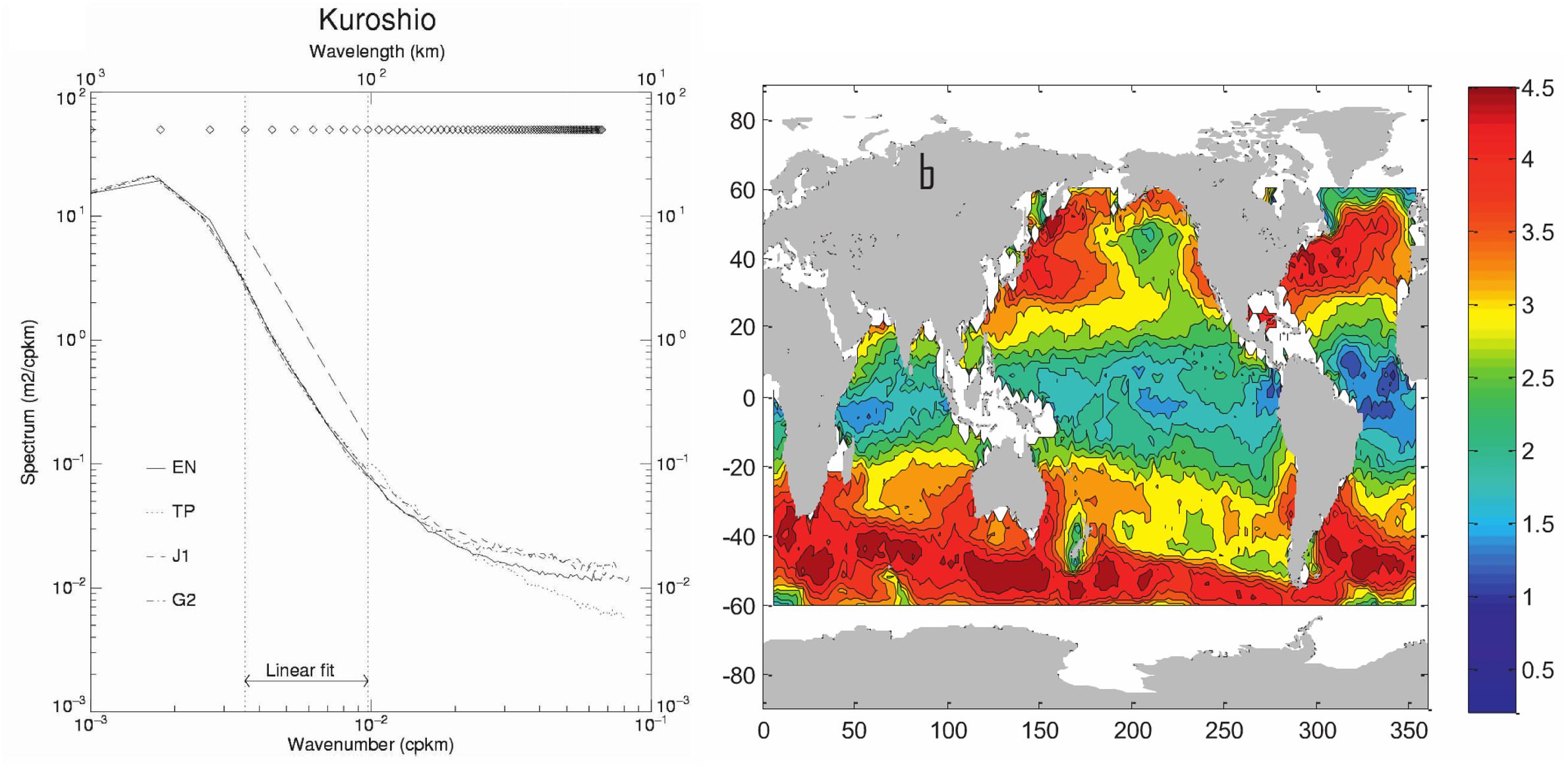
Figure 1. (Left) SSH wavenumber spectra in the Kuroshio region from four altimetric missions. The –11/3 slope is shown by the dashed line (from panel b of Figure 1 in Le Traon et al., 2008). (Right) Global SSH wavenumber spectral slopes (with a reversed sign) in the 70–250 km range (from panel b of Figure 3 in Xu and Fu, 2012) (copyright 2012, American Meteorological Society).

Regardless of the exact dynamical regime, steep along-track SSH spectra in energetic regions are consistent with geostrophic turbulence over the mesoscale range (70–250 km). However, the shallower spectra in low-energy regions remain puzzling and may result from multiple processes, including direct wind forcing (Le Traon et al., 1990), or internal tides and internal waves (Richman et al., 2012; Callies and Ferrari, 2013; Dufau et al., 2016; Rocha et al., 2016; Tchilibou et al., 2018). The full 2D SSH observations of the mesoscale and internal tide/internal wave fields are needed to better understand these regional and seasonal variations.

SWOT Measurement System

Measurement Technique, Ocean Data Products

Surface Water and Ocean Topography will use SAR-interferometric technology to observe 2D images of SSH and surface roughness over two 50-km wide swaths with a 20 km nadir gap (see Figure 2A). A conventional Jason-class nadir altimeter provides measurements in the central gap. SAR-interferometry has been demonstrated with SRTM on the Space Shuttle, and with Cryosat-2 SARIN mode for the polar ice caps. SWOT improves on these concepts: it is designed to have lower noise and uses different polarizations and antenna patterns to clearly distinguish the signals coming from the left-right swaths. The details of the SAR-interferometric technique are explained in Rodriguez et al. (2018).

FIGURE 2

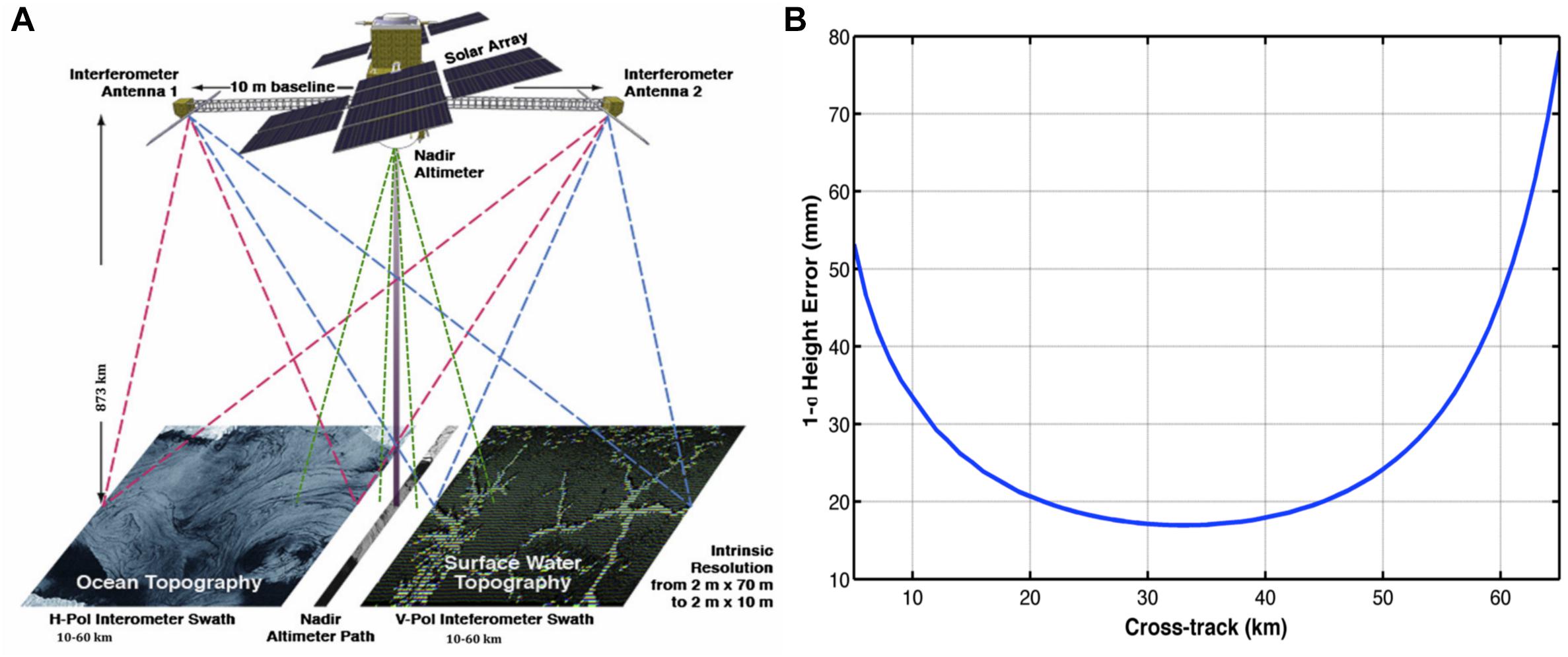
Figure 2. (A) Schematic of the SWOT measurement technique using the KaRIn instrument for SAR-interferometry over the two swaths, and a Jason-class nadir altimeter in the gap. (B) The standard deviation of the ocean height error performance at 1 km × 1 km due to all the random errors (in mm) as a function of distance across the swath for a 2-m significant wave height. The swath-averaged (10 to 60 km) height error is 2.4 cm (Credits: NASA-JPL).

Surface Water and Ocean Topography uses SAR processing to refine the alongtrack resolution of the return signal; the interferometric processing refines the cross-track resolution. The SWOT SAR-KaRIn instrument provides a basic measurement resolution of 2.5 m alongtrack, ranging from 70 m in the near-nadir swath to 10 m in the far swath. Over the 70% of the Earth’s surface covered by oceans, SWOT’s huge volume of data cannot be downloaded from the satellite. Instead, so-called “low-resolution” data will be pre-processed onboard, and building blocks of nine interferograms at 250 m posting (and 500 m resolution) will be downloaded from each antenna. Other parameters that are useful for the surface roughness and front detection, such as the 250 m resolution backscatter images, will also be downloaded. The interferometric data will be combined through a geolocation and height calculation into a 250 m × 250 m expert SSH product in swath coordinates. Most scientists will use a 2 km × 2 km product available in geographically fixed coordinates. This basic 2 km resolution product will be separated into three file types: a “light” SSH and SSH anomaly product; a wind-wave-sigma0 product; and a full SSH product with all geophysical corrections included. More details on these different data products are given at https://www.aviso.altimetry.fr/en/missions/future-missions/swot/data-products.html.

Measurement Errors, SWOT Simulator, and Effective Spatial Resolution

The SWOT SAR-interferometry measurement is designed to have small instrument noise to meet the stringent requirement of 2.7 cm in rms noise for 1 km² pixels. This leads to 2 cm²/cycle/km² noise over the oceans at short wavelengths, for a 2 m SWH average sea-state, calculated over 7.5 km × 7.5 km averages (to resolve the 15 km Nyquist wavelength). For comparison, the noise level for the Jason series is around 100 cm²/cyc/km² at 1 Hz, i.e., averaged over the 1 s oval footprint or roughly 100 km². The SWOT instrument measurement will be very precise. For the first time for an altimetric mission, the error budget is also set in terms of wavenumber, so the instrument design must meet long wavelength and short wavelength goals (see Figure 3). This is unprecedented for an altimeter mission. By using the wavenumber spectrum, the requirement effectively requires that the measurements be analyzed over a range of spatial scales and thus imposes a more stringent test on the satellite performance than the variance-based validation for previous altimeter missions. SWOT needs to account for standard altimetric SSH range errors, but in wavenumber space. SWOT also has specific errors associated with the interferometric calculation, including roll errors, interferometric phase and range errors, baseline errors, radial velocity errors from observing a moving target, and wave effects. The description of these errors and techniques to reduce them are detailed in the SWOT Error budget and performance document (Esteban-Fernandez, 2017) and discussed in Rodriguez et al. (2018) and Chelton et al. (2019). Most importantly, it is the random errors in the KaRIn measurements over short wavelengths that eventually determines the SWOT resolution.

FIGURE 3

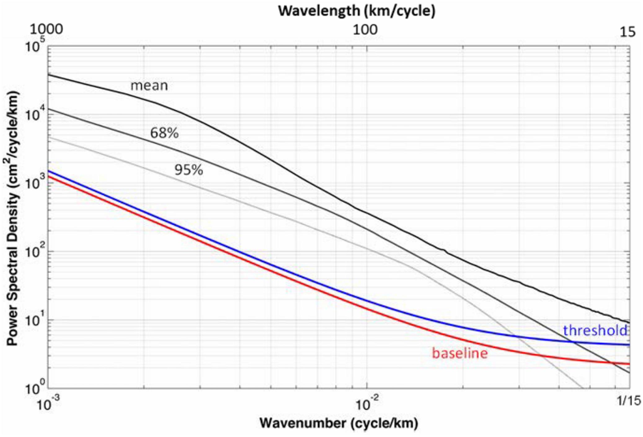
Figure 3. SSH baseline requirement spectrum (red curve) as a function of wavenumber represented by an empirical function, E(k) = 2 + 0.00125 k^-2, where k represents along-track wavenumber. The blue curve is the threshold requirement. Shown for reference is the global mean SSH spectrum estimated from the Jason-1 and Jason-2 observations (thick black line), the lower boundary of 68% of the spectral values (the thin black line), and the lower boundary of 95% of the spectral values (the gray line). The blue and red lines represent a swath-average performance, and intersect the baseline spectrum at ∼15 km (68%) and ∼30 km (95%), respectively (Desai, 2018; Credits: NASA-JPL).

Surface Water and Ocean Topography random errors across the swath are not uniform (Figure 2B) being larger near the edges, smaller in the center. These errors vary spatially and temporally, influenced by the surface wave and roughness conditions, as with all altimeter missions. Predictions of the SWOT sampling and noise levels are available for ocean studies using a simulator at: https://github.com/SWOTsimulator/swotsimulator.git. Since the total SWOT error has different causes and space-time structure, techniques are being developed to estimate the noise patterns using cross-spectral methods (Ubelmann et al., 2018) and remove them using advanced de-noising techniques (e.g., Gómez-Navarro et al., 2018). This is needed since any ocean studies requiring geostrophic velocity or vorticity calculations will amplify the small-scale noise when taking the first or second derivatives of SSH.

The SWOT noise will also affect the effective spatial resolution of ocean signals, since higher noise levels will hide the smaller-scale signals. Global estimates of the SWOT noise, including a wave-dependency, have revealed the spatial distribution of this effective resolution (Dufau et al., 2016; Wang et al., 2019), i.e., the minimum spatial scale where the signal-to-noise is greater than 1. The estimated effective resolution has a geographic and seasonal dependence. It increases from about 15 km in low latitudes to ∼30–45 km in mid- and high-latitudes and is generally greater in summer than winter, but with a large geographic variation (Figure 4). Both eddy and internal gravity wave/tide signals contribute significantly to these scale variations. For example, in Figure 4D, the reversed seasonality in the southern hemisphere is due to a dominance of internal gravity waves in the subtropics in summer with low measurement noise, and dominant submesoscale energy and higher noise in winter across the Circumpolar Current. This effective resolution of the different signals and noise needs to be taken into account when combining SWOT observations with in situ data or models in regional analyses.

FIGURE 4

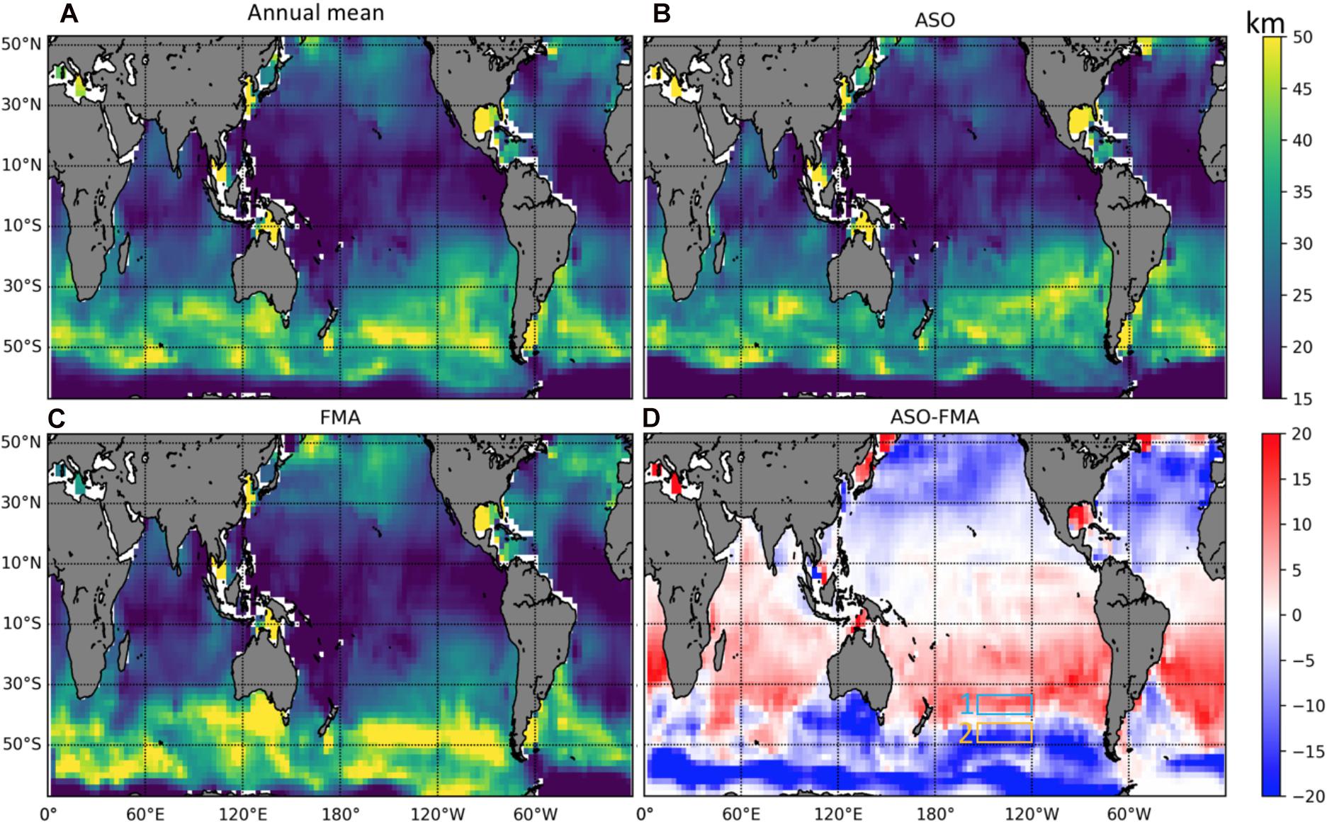
Figure 4. SWOT effective spatial resolution (signal above noise) estimated from a model and simulated noise (A) averaged annually, (B) in August–September–October (ASO), (C) in February–March–April (FMA). The seasonal change (ASO-FMA) is shown in (D) (after Wang et al., 2019; copyright 2019, American Meteorological Society).

Orbits – Science Phase and Fast
Sampling Phase

The SWOT launch is planned for September 2021. SWOT will spend the first 6 months in its “calibration orbit,” where the satellite passes over the same site every day to calibrate the satellite parameters (groundtrack shown in Figure 5A). The first 3 months of this orbit are to adjust and calibrate the instrument parameters, the second 3 months (late December 2021 to late March 2022) will be available for science studies, including studies of rapidly evolving small-scale ocean dynamics. SWOT will then continue in its nominal 21-day repeat orbit for 3-years, from April 2022 to March 2025. Details of the nominal and calibration orbits in different formats can be found at: https://www.aviso.altimetry.fr/en/missions/future-missions/swot/orbit.html.

FIGURE 5

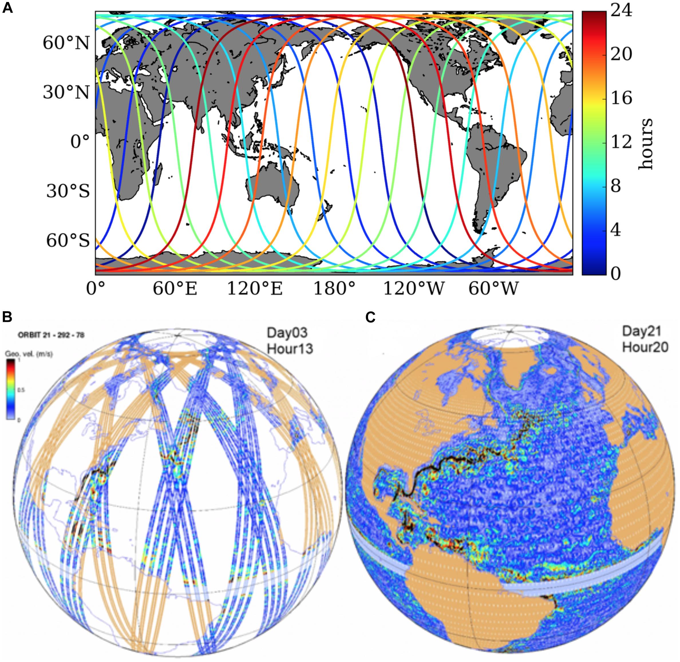
Figure 5. (A) Global coverage of SWOT’s 1-day orbit. Color shows the time in hours of each pass (Wang et al., 2018) ©Copyright [2018] American Meteorological Society (AMS). SWOT coverage in its 21-day orbit after 3 days (B) and 21 days (C). The color shows model simulations of SSH at the measurement time (after Morrow et al., 2018a; copyright 2018, CreateSpace Independent Publishing Platform).

The SWOT Science Definition Team investigated the SWOT nominal orbit coverage in detail. Any orbit choice involves a tradeoff between good spatial coverage and temporal coverage. The two major communities using SWOT observations had different objectives – hydrologists needed global coverage of the smallest lakes and rivers on a monthly time scale. Oceanographers needed coverage of the small, rapidly evolving, ocean scales. The final science phase orbit covers most of the oceans up to 78°N and S (inclination of 77.6°), at 890.6 km altitude on a 21-day repeat orbit (Figure 5C). Figure 5B shows the sampling over the North Atlantic Ocean after 3-days; after 10-days there is loose global coverage for the mesoscales, and over the next 11–21 days the entire pattern shifts westward to fill the gaps, giving near global coverage after the full cycle (see Figure 5C). SWOT has a non-sun-synchronous orbit. Its inclination and repeat sampling were specifically chosen to resolve the major tidal constituents, needed to improve the coastal, high-latitude, and internal tides.

Validating the Ocean Vertical Contribution to SWOT Wavenumber Spectra

SWOT Calibration and Validation on Wavenumber Spectrum

Calibration and validation is an important component of any satellite mission. The instrument performance can be assessed by comparing measurements to the precise ground truth. For an exploratory mission such as SWOT, CalVal is crucially important. During the CalVal phase, the SWOT orbit will be on a fast-repeat (1-day) orbit cycle, providing daily revisits along the same ground track at the expense of the spatial coverage (Figure 5A). Two overpasses will be made every day at the crossover locations, making these locations ideal for CalVal.

For CalVal purposes, the difference between SWOT measurements and ground truth is defined as error and specified in terms of the along-track wavenumber spectrum (Figure 3). SWOT measurement errors are discussed in Section “Measurement Errors, SWOT Simulator, and Effective Spatial Resolution.” The requirement covers a large span of wavelengths, extending from 15 km to 1,000 km. The onboard Jason-class nadir altimeter will be used for the long wavelength CalVal (e.g., >120 km suggested by Wang and Fu, 2019). The nadir-altimeter, which benefits from the heritage and successful cross-calibration of numerous previous altimetry missions, has a well understood instrument performance and can serve as the reference for long wavelengths. Cross-calibration with other nadir missions (e.g., Sentinel-3, Jason-CS) will also be performed. The ground measurement can then focus on a smaller spatial range [15–O(100) km].

Sea surface height wavenumber spectra over 15–120 km wavelengths can be verified using airborne Lidar (e.g., Melville et al., 2016) and in situ observations. Unfortunately, no in situ observations exist today that can provide a reliable SSH wavenumber spectrum for these wavelengths. Determining the small-scale SSH wavenumber spectrum is a critical task for the SWOT in situ CalVal field campaign.

Due to high-frequency internal tides and waves, the construction of a ground truth that measures 15–120 km wavelengths will rely on simultaneous high-frequency (hourly at least) sampling over 120 km distance. An array of global position system (GPS) or Conductivity-Temperature-Depth (CTD) moorings is required. Wang et al. (2018) used an Observing System Simulation Experiment (OSSE) to demonstrate the ability of moorings to meet the requirement. The GPS’s capability is undergoing testing near the Harvest platform at the time of writing.

Global position system measures the true ocean surface height as seen by satellite, while the SSH reconstruction by CTD moorings relates to the ocean dynamic topography, the component that is meaningful for studying ocean circulation. GPS can be referred to as a direct geodetic validation, and CTD moorings are an indirect oceanographic validation. The primary oceanographic objectives of the SWOT mission are “to characterize the ocean mesoscale and submesoscale circulation determined from the ocean surface topography at spatial resolutions of 15 km (for 68% of the ocean)” (Fu et al., 2012). It is important to have both geodetic and oceanographic components evaluated at the CalVal site simultaneously in order to connect the satellite measurements with the interior ocean physics.

SWOT Validation Using in situ Observations

The SSH, η, is related to three dynamical terms through the hydrostatic equation:

$$\text{η}=\frac{p_b^{\text{'}}}{{\text{ρ}}_{0}g}-\frac{p_a}{{\text{ρ}}_{0}g}-{\displaystyle {\int }_{\text{-}H}^{\text{0}}\frac{{\text{ρ}}^{\text{'}}}{{\text{ρ}}_{\text{0}}}}dz(1)$$

where p_a is the surface atmospheric pressure loading, p_b the bottom pressure and $p_b^{\text{'}}\cong p_b-p_{0}gH$ the bottom pressure anomaly. The term ${\displaystyle {\int }_0^{\text{η}}\frac{{\text{ρ}}^1}{{\text{ρ}}_0}}dz$ has been neglected because η << H in the open ocean. In real satellite measurements, additional terms due to the geoid, measurement errors, and noise will appear on the right-hand side of the equation but are dynamically irrelevant and often corrected. The atmospheric loading, i.e., the inverted barometer response (Doodson, 1924), is routinely corrected using atmospheric reanalysis. Barotropic signals appear in the bottom pressure and are believed to have large spatial scales, greater than 120 km in wavelength in the open ocean. The third term, the steric height (or dynamic height with a factor of g difference), reflects ocean interior dynamics and is the most important variable for altimetric oceanography.

In situ oceanographic validation means that we need to compare the satellite measurement to the dynamic height reconstructed from the hydrographic measurements and understand their connection in terms of spatial structures such as wavenumber spectrum.

The CalVal Site Near California

Among the 14 crossover locations in mid-latitudes (∼35°N), the one in the California Current System (CCS) about 300 km off Monterey has been proposed as the main SWOT CalVal site (125.4W, 35.7N). This location belongs to a family of oceanic eastern boundary currents. The CCS is one of the most well studied boundary currents due to its socio-economic importance. The first concentrated investigation of this region dates back to 1937 (Sverdrup and Fleming, 1941).

Dynamic height has long been used to study the circulation of the CCS (e.g., Sverdrup and Fleming, 1941; Reid, 1961; Wyllie, 1966). One particular example is Bernstein et al. (1977), who studied California Current eddy formation using dynamic height calculated from California Cooperative Oceanic Fisheries Investigations (CalCOFI) observations and satellite images. The dynamic height used in that study was based on hydrographic profiles of the upper 500 m. Results showed good agreement between the circulation pattern in the 500 m-dynamic height and the mesoscale eddies identified in satellite infrared imageries. Since then, numerous field programs have taken advantage of the abundance of both in situ observations and higher resolution satellite measurements (e.g., Brink and Cowles, 1991).

Hydrographic profiles from the upper 500 m have been widely used for dynamic height calculations and may well account for the majority of the total variability, but we do not yet know whether they are sufficient to meet the SWOT requirement. Deep eddies have been observed occasionally (Collins et al., 2013). In addition, high-frequency internal tides and waves may have deep-reaching structure. The combination of deep-reaching dynamics, the large span of the spatial scales, and the fast-changing waves impose significant challenges for validating the SWOT SSH snapshots.

Wang et al. (2018) OSSE used a high-resolution (1/48° in horizontal and 90 levels in vertical) global ocean simulation with tidal forcing, and analyzed the contribution of upper-ocean density variations to the SSH wavenumber spectrum. They showed that the upper 570 m accounts for more than 70% of the variance of SSH for all wavelengths between 15 and 150 km near the CalVal site in CCS. The remaining 30% variance not captured by the upper ocean does not result in an error exceeding the SWOT baseline requirement. The results in wavenumber space are shown in Figure 6, where the error (blue lines), defined as the difference between the model SSH and the dynamic height calculated from the 570 m synthetic mooring observations, is near or below the SWOT baseline requirement. Observing the deeper ocean leads to a better reconstruction of the truth (not shown). Sampling the upper 570 m of the ocean was a compromise of cost versus performance based on a preliminary study. The design of the in situ CalVal system has been evolving, leading to a new plan of using full-depth moorings of sensors to reach over 90% accuracy.

FIGURE 6

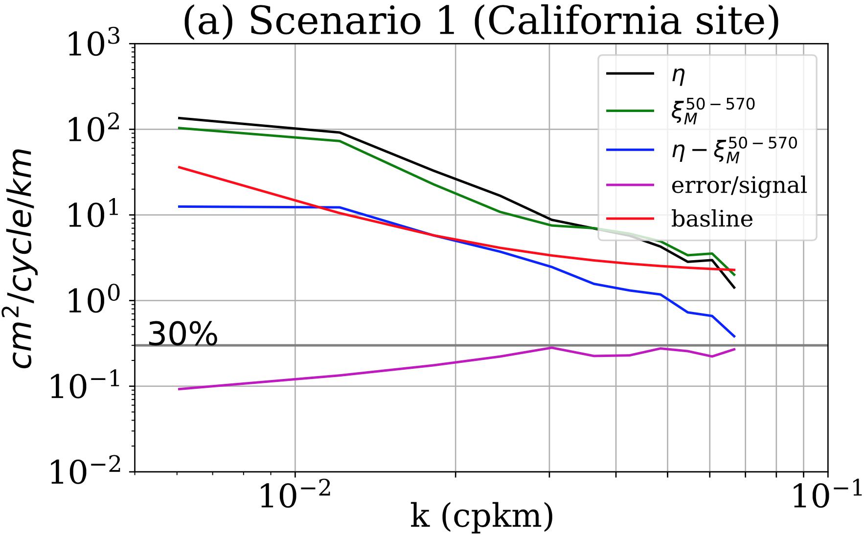
Figure 6. The wavenumber power spectrum density of the true SSH anomaly η (black), the mooring reconstruction ξ_M (green), the residual η – ξ_M (blue), the error-to-signal ratio (purple), and the baseline (red). Visual guide of the 30% (0.3) level (horizontal line) (Wang et al., 2018; copyright 2018, American Meteorological Society).

In summary, the stringent SWOT science requirement on the SSH wavenumber spectrum requires a comprehensive in situ field program for CalVal. This will provide an opportunity to build a larger oceanography science field campaign by taking advantage of both the large SWOT CalVal instrument array and the simultaneous SWOT swath SSH measurement. The expanded field program, in turn, will enhance our understanding of the future SWOT data and their connection to ocean dynamics.

As mentioned in the introduction, other science validation studies are planned during the fast sampling phase in different dynamical regimes in both hemispheres, so in different seasons. These are described in more detail in the accompanying OceanObs review paper “Resolving the fine scales in space and time: interdisciplinary science opportunity during the SWOT fast sampling phase and beyond.”

Opportunities for Multi-Satellite Surface Characteristics of Fine-Scale Fronts and Eddies

Frontal Signatures in Optical and Radar Data

Satellite optical and radar measurements often reveal sea surface roughness changes at sub-kilometer scales, mostly under low to moderate wind conditions (e.g., Alpers, 1985; Yoder et al., 1994). These surface roughness changes can be traced by surface current gradients, related to internal waves and/or surfactant lines created by surface velocity convergences. They typically occur with sharp gradients of temperature and/or ocean color. Efforts have been made to interpret surface roughness gradients quantitatively (e.g., Kudryavtsev et al., 2014; Rascle et al., 2016, 2017). They confirm that horizontal convergence and shear estimated from in situ drifters are generally consistent with the theoretical wave action equation (e.g., Kudryavtsev et al., 2005, 2012). This equation predicts how current gradients influence the amplitude of short gravity waves that propagate in different directions, from which a surface optical reflectance or radar cross section can be estimated. When several viewing angles are available, optical or radar measurements can be inverted to yield both the amplitude and direction of the surface current gradient.

Surface Water and Ocean Topography backscatter variations will be released on a 250-m resolution grid, as discussed in Section “SWOT Measurement System,” and are expected to provide a more nuanced view of frontal scale variations than will be available from the processed SSH data (Figure 7). To leading order, backscatter variations will inform us about local changes related to the omni-directional short scale mean squared slopes. As anticipated [e.g., Eq. (3) in Kudryavtsev et al., 2012], this can offer a direct link between SWOT’s SSH mapping capabilities and the divergence/convergence of the sea surface current field. We expect that SWOT’s combined measurements (SSH, surface wave mean squared slopes) will thus offer an unprecedented capability to trace intense cross-frontal dynamics and vertical motions, including spiraling eddies (Munk et al., 2000; Eldevik and Dysthe, 2002), internal waves and cold-filaments (McWilliams et al., 2009).

FIGURE 7

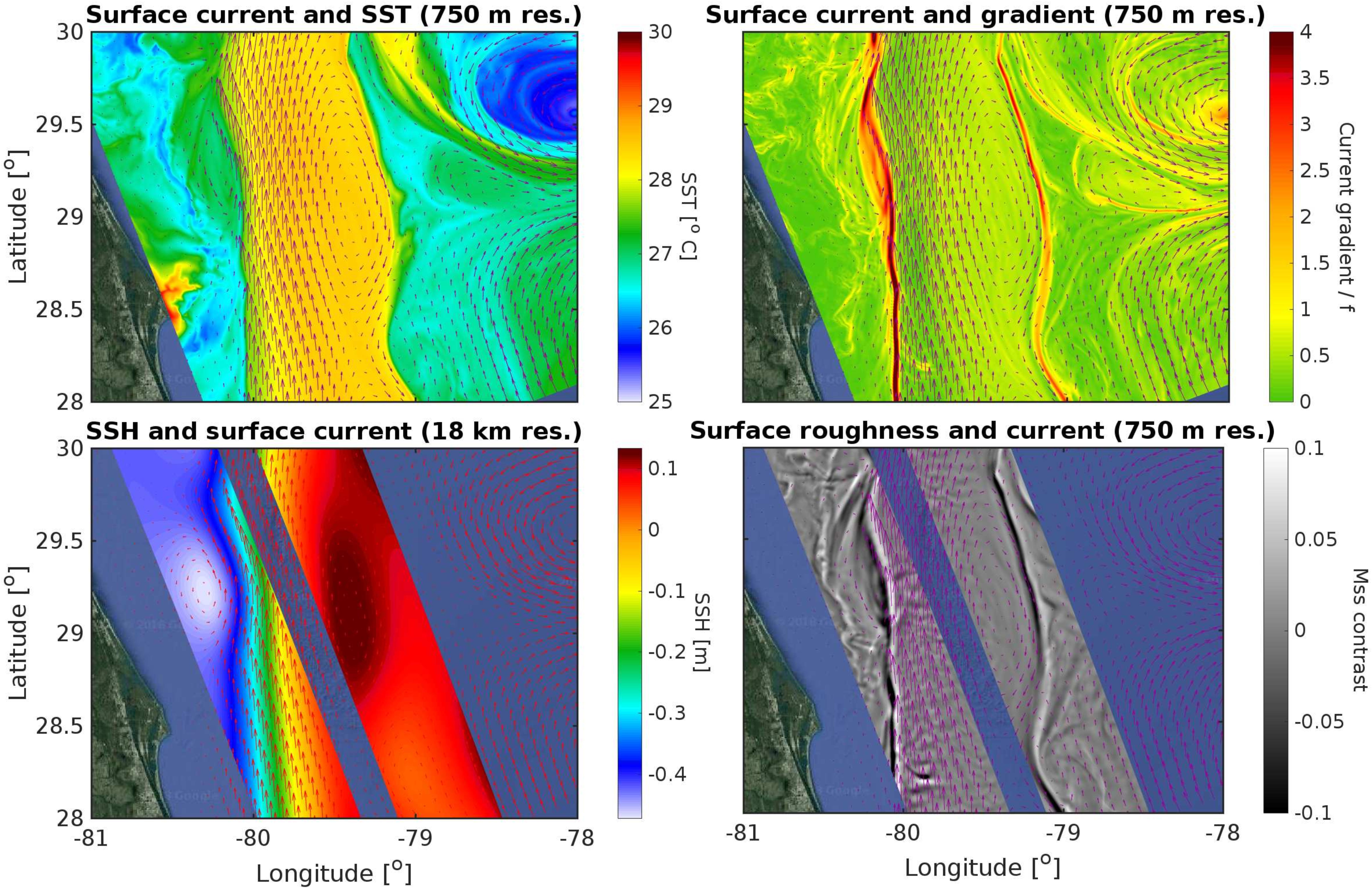
Figure 7. Numerical simulations over the Gulf Stream to illustrate the possible synergetic use of SWOT SSH (averaged at 18 km, bottom left) and SWOT backscatter (averaged at 750 m, bottom right). Geostrophy at 18 km resolution does not reproduce frontal structures (bottom left, red arrows), with weak current gradients, always well below the Coriolis frequency f (not shown). The backscatter at sub-kilometer resolution (bottom right) provides information on the location and amplitude of the intense current gradients (top right) (Credits: Ifremer).

Sea State Modification Across Fronts and Eddies – Today and With SWOT: Issues and Opportunities

Winds over the ocean can be gusty, with intermittent features and small-scale spatial variations that modulate larger-scale patterns of variability. If winds move at the same velocity as ocean currents, they have no net impact on the ocean surface: the net wind-stress exerted by the wind on the ocean depends on the differential velocity between the wind flow at the surface and the ocean currents just below (e.g., Liu et al., 1979; Kelly et al., 2005). Wind stress can generate surface waves, which propagate horizontally through the ocean, modulated by ocean currents (e.g., Ardhuin et al., 2017). Some of the energy input to the ocean by the wind drives the large-scale ocean circulation; some energy is dissipated within the wave field or through breaking along the shore and has little net impact on the large-scale ocean circulation. One of the critical questions for physical oceanography has been to understand the interactions of winds with waves and small-scale ocean currents. SWOT’s resolution of the backscatter associated with the wave field and its sea surface height measurements will offer valuable contributions to the study of wave–current interactions, and the addition of separate satellite missions to measure currents, waves, and wind will enable more detailed assessment of the mechanisms driving wind power input to the ocean.

Whereas the surface roughness is defined by short gravity waves (wavelengths around 1 m) with variations of the order of 10% due to currents, the effect of currents on dominant wind-waves can be much larger (Kenyon, 1971; Romero et al., 2017). Even in the absence of non-linearities, waves traveling through a field of varying surface currents can exhibit random focusing, possibly leading to extremely high wave intensification (e.g., Kudryavtsev et al., 2017; Quilfen et al., 2018). Such an effect is generally non-localized with the surface current changes, but is related to the ratio between surface current gradient (vorticity) and wave group velocity. From the conservation of action, the spatial variability of the significant wave height (SWH) will thus be linked to the surface kinetic energy of the current (Ardhuin et al., 2017). This variability of SWH can be a source of noise in the SSH estimation, through the sea-state bias estimation. It is also an opportunity to better characterize small scale currents, provided that the SWH (from the nadir instrument, and very near nadir estimates) or other estimated sea state parameters are available (Quilfen et al., 2018). Also, building on the long-range propagation of ocean swells (Collard et al., 2009), there is a great potential to assess refraction effects estimated from SWOT’s 2D wave-mapping capabilities, in order to improve wave forecasts and comparisons with other (satellite, in situ) sea state measurements.

The China-France Oceanography Satellite (CFOSAT), which will measure winds and waves starting in 2018, as well as proposed satellites, including the European Space Agency’s Sea surface Kinematics Multiscale monitoring (SKIM) mission and a NASA concept for a Winds and Currents Mission (WaCM), all offer the potential to complement SWOT with coincident measurements of surface currents plus waves and/or winds. Aircraft measurements from Lidar, and from the airborne version of SWOT – AirSWOT, and from DopplerScat, a suborbital WaCM prototype, have all demonstrated the alignment of winds and currents. SWOT’s high-resolution Doppler Centroid product, in combination with microwave-derived wind, wave, and current measurements from Lidar, CFOSAT, SKIM, and/or WaCM have the potential to highlight the fine-scale wind–wave–current interactions through which momentum is transferred between the atmosphere and the ocean.

Fronts, Ocean Color, and Structuring Biomass

Ocean fronts can be characterized by strong vertical velocities, in addition to supporting sharp gradients in temperature, current speed and other ocean properties. The vertical velocities at fronts can bring nutrients to the ocean surface and stimulate primary production, and play an important role in marine ecosystems. Ocean color data highlight the filamented structures of chlorophyll-a at the ocean surface (e.g., Kahru et al., 2007), which can be extremely narrow, suggesting the importance of both horizontal and vertical velocities in governing biological productivity at scales smaller than the eddy scale: the sub-mesoscale (Lévy et al., 2001, 2012b; Mahadevan, 2016), with possible effects propagating to higher trophic levels (Lehahn et al., 2018). However, the data to analyze these processes have not been available in a consistent global form. Ocean color data and high-resolution SST are not available in cloudy conditions, and therefore both are highly patchy, SAR imagery is not archived globally, and other sensors have not achieved high-resolution sampling in two dimensions. SWOT’s global swath sampling, particularly if used in combination with other sensors, will provide a means to assess the structure of waves and SSH gradients at ocean fronts in the context of chlorophyll-a color measurements.

From SWOT Observations to 2D SSH and 3D Fields

Improved 2D Mapping of Fine-Scale SSH With SWOT and Nadir Altimeters

Present-day 2D maps of SSH, derived from a constellation of two to five nadir altimeters using statistical, static interpolation techniques (Dibarboure et al., 2011), do not resolve scales smaller than 150–200 km in the mid latitudes. SWOT will provide an unprecedented opportunity to increase spatial resolution, but the mapping method must be adapted. Due to the mismatch between spatial and temporal coverage of SWOT, fast and small-scale dynamical processes may develop and move unobserved between two passes, possibly leading to a poor mapping of SSH. This is suggested by Figure 8, showing that ocean decorrelation times decreases dramatically as the spatial scales decrease. At 180 km, the decorrelation time is about 10 days which is the typical revisit of nadir altimetry. However, at 15 km, the decorrelation time is below 1 day, much shorter than the revisit of SWOT. For this reason, temporal interpolation in mapped SSH data should be revisited, from a static statistical approach to a dynamical approach, to better represent the small scales’ evolution.

FIGURE 8

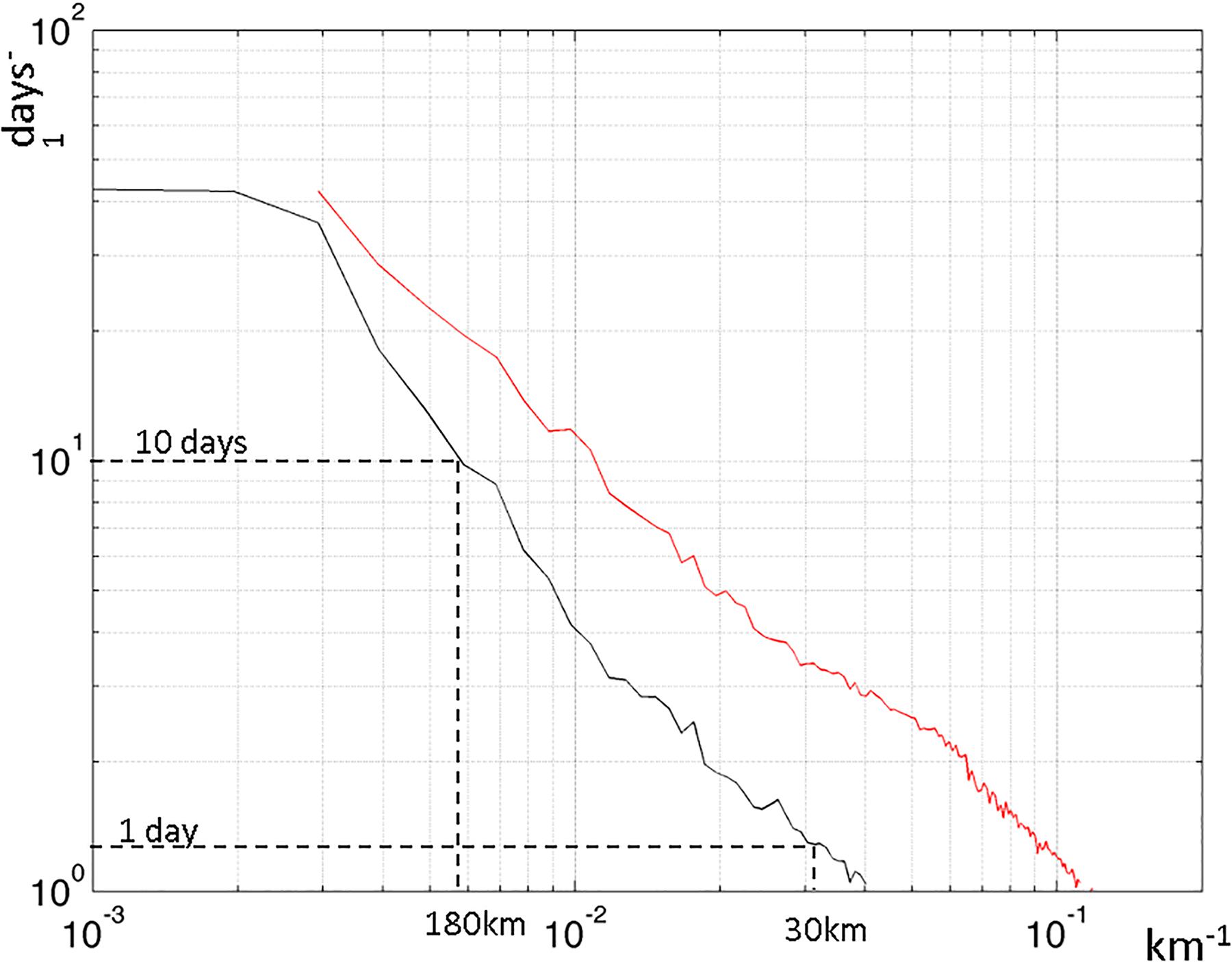
Figure 8. Black curve: decorrelation time as a function of wavelength (shown in inverse log scale, per day and/km, respectively) estimated from an MITgcm simulation in the North Atlantic. Red curve: Decorrelation time when we subtract the 1-layer Quasi-Geostrophic evolution (Credits: NASA-JPL).

A proof-of-concept study of dynamical interpolation has been carried out by Ubelmann et al. (2015), quantifying the improvements in the reconstruction 2D of SSH fields with a 1-layer Quasi-Geostrophic model relying on a single parameter: the Rossby radius. The simulated results suggest significant improvements (up to 30% error reduction and 20% gain in resolution) in energetic western boundary currents. Ubelmann et al. (2016) implemented the method to use simulated observations. Figure 9 illustrates the results with simulated SWOT data. The limitation of the statistical interpolation technique, and the benefits of a dynamical approach are clear on this image: Two well-defined eddies are detected by SWOT at two different times separated by 7 days (top panel). They have moved during this period. The SSH field estimated at an intermediate time using the statistical interpolation technique shows sluggish, deformed eddies (bottom panel, center), since they result from a weighted average of the two initial images. The eddies’ integrity is much better represented using a dynamical interpolation technique (bottom panel, right).

FIGURE 9

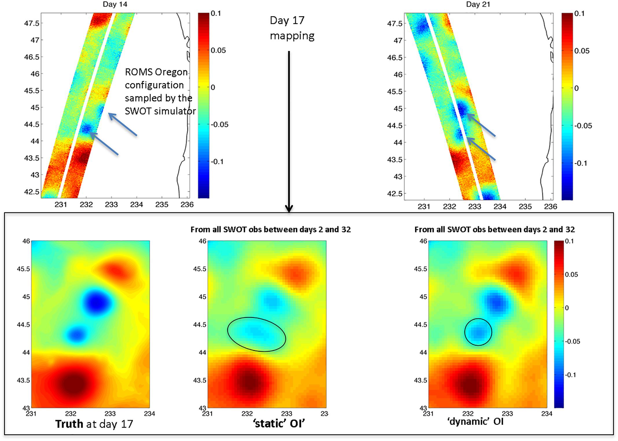
Figure 9. Upper panels: SWOT Level 3 data shown for day 14 and day 21 in a simulation off the Oregon coast. Lower panels: from left to right: reference field, analyzed field with static optimal interpolation and analyzed field with dynamic interpolation on day 17, processing all data available between days 7 and 27 (Credits: NASA-JPL).

Another dynamical approach where the time interpolation relies upon quasi-geostrophic dynamics is also explored, where simulated SWOT observations are combined with the model through a back-and-forth nudging approach (Auroux and Blum, 2008; Ruggiero et al., 2015): the model is iteratively run forward and backward over a fixed time window, and gently nudged toward the observations at every time step with an elastic restoring force. Results indicate that this approach successfully reconstructs the SSH field in the full space and time domain considered.

Efforts are continuing to investigate dynamical mapping strategies to draw the maximum benefits from SWOT and alongtrack altimetry’s fine-scale SSH. Approaches reported here are encouraging, but have been explored by ignoring or minimizing the structured component of SWOT errors (roll, baseline, phase and range errors in particular). Dealing with such errors is part of ongoing work, and a major challenge for the inclusion of SWOT in the 2D mapping of SSH.

3D Projection From Surface Satellite SSH and SST/Density Observations

Surface Water and Ocean Topography sea level provides an estimate of pressure at the ocean surface which may be extrapolated downward in the water column and provide an estimate of the circulation at depth. Assimilation of SWOT and other available data with realistic 3D primitive equations numerical models may achieve this albeit at a large computational cost (see section “Assimilation of SWOT Data”).

For the larger mesoscales, empirical statistical correlations have been developed between altimetric sea level observations and collocated Argo dynamic height at depth (Guinehut et al., 2006, 2012). Owing to the geostrophic relationship between currents and pressure, the observed low modal vertical structure of currents may be leveraged to extrapolate sea level downward (Wunsch, 1997; Sanchez de La Lama et al., 2016), and the resulting vertical structure may be justified dynamically (Smith and Vallis, 2001). We still need to explore how these approaches extend to the newly resolved 2D scales of SWOT.

Other approaches have relied on quasi-geostrophy which is the relevant dynamical framework for mesoscale motions. At mesoscales, primitive equations (for velocity, temperature, salinity, etc.) can indeed be recast in a simpler system where the only state variable is potential vorticity (PV), which binds fluctuations of currents and density. Previous studies have reconstructed 3D fields from a combination of in situ and satellite observations, including the estimation of vertical velocities, through the quasi-geostrophic approximation (Ruiz et al., 2009; Buongiorno Nardelli et al., 2012; Pascual et al., 2015; Mason et al., 2017; Barceló-Llull et al., 2018). A key problem when trying to obtain accurate estimates of the vertical exchanges from in situ and remote sensing data is related to the availability of high-resolution data. In this context, SWOT will make an unprecedented contribution when combined with in situ observations.

Assuming specific relationships between SSH, SST and PV, different studies have shown the feasibility of inverting oceanic currents in 3D from these surface observations in both idealized and realistic settings (Lapeyre and Klein, 2006; Klein et al., 2009; Ponte and Klein, 2013; Wang et al., 2013; Qiu et al., 2016) (Figure 10). Further theoretical advances are needed to account for vertical variations of PV that are not directly related to surface variables (Lapeyre, 2009; Fresnay et al., 2018). As for the 2D mapping of SWOT data (see section “Improved 2D Mapping of Fine-Scale SSH With SWOT and Nadir Altimeters”), using the predictive nature of quasi-geostrophy may also allow progress in the future.

FIGURE 10

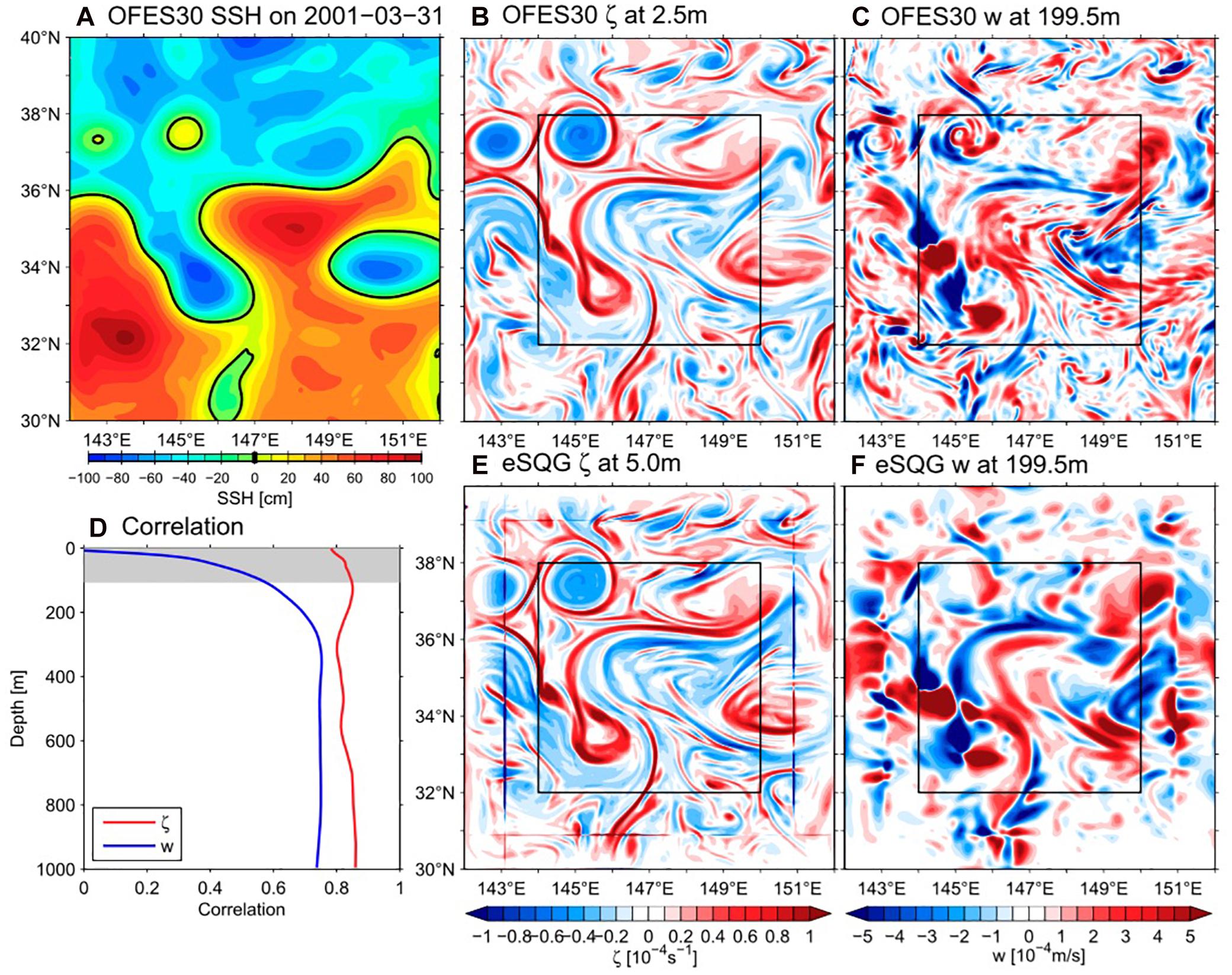
Figure 10. (A) Numerical simulation sea level on March 31, 2001. (B) Relative vorticity at 2.5 m and (C) vertical velocity w at 199.5 m from the numerical simulation. (E) Relative vorticity at 5.0 m and (F) w at 199.5 m reconstructed based on sea level according to effective SQG. (D) Linear correlation coefficients for relative vorticity (red line) and w (blue line) between the original and reconstructed fields as a function of depth. Gray shade denotes the mixed layer depth averaged in the reconstruction region of 32°–38°N and 144°–150°E (see Qiu et al., 2016 for details; copyright 2016, American Meteorological Society).

Many of the outstanding issues and opportunities (3D circulation reconstruction, balanced/internal wave disentanglement) will require that we combine SWOT sea level observations with other types of observations. Statistical approaches show that the combination of sea surface temperature observations with sea level can improve reconstructions of 3D pressure and currents at mesoscales (Mulet et al., 2012). Surface tracers which have been stirred by advective currents have been used to improve finer-scale surface current estimates (Rio et al., 2016) or to disentangle internal waves from balanced contributions to sea level (Ponte et al., 2017). Much remains to be investigated about the relevant observations needed, as well as the development and performance assessment of methods for propagating SWOT observations into the ocean interior, via statistics, dynamics or both.

Assimilation of SWOT Data

Surface Water and Ocean Topography will provide very high resolution observations along its swaths but will not be able to observe the evolution of the high frequency signals (periods < 20 days). The assimilation of SWOT data in ocean models will be instrumental to control smaller scales (<100 km) that are not well constrained by conventional altimeters. The most impacted fields will be surface and intermediate horizontal velocities, which directly impact on key applications such as marine safety, pollution monitoring, ship routing, and the offshore industry. A better constraint on vertical velocities will also directly impact biogeochemical applications.

The challenge of assimilating SWOT is multi-facetted. We can identify four conditions to be fulfilled to draw maximum benefit from SWOT data assimilation:

(i) The assimilative model should have a spatial resolution comparable to SWOT. This is by itself a big challenge: running a basin-scale model at SWOT resolution on present-day supercomputers is computationally extremely expensive. Computational complexity issues are further aggravated in data assimilation mode.

(ii) The model should represent all the physical processes affecting SWOT data. As mentioned earlier, dealing with internal tides in SWOT data is a particularly difficult and open question. Internal tides are even more challenging for SWOT assimilation since their signature on SSH can exhibit long spatial coherence, whereas some assimilation methods work under the assumption that observations have a local signature only.

(iii) SWOT’s temporal coverage should fit the characteristic time scales of the model’s dynamics, yet this will not be the case. To draw maximum benefit from SWOT’s spatial resolution while minimizing the adverse effects of its temporal resolution, SWOT data will have to be assimilated in combination with conventional along-track altimeters and in situ observations (e.g., Argo).

(iv) SWOT data should be integrally assimilated. It is common, when dense data are assimilated, to thin the observation data set. A main objective of data thinning is to avoid data with correlated errors, simply because data assimilation systems are not designed for such data.

Different groups in the SWOT Science Team are working on these issues. To address (i) and (ii) above, the approach followed by Mercator Ocean is to develop/test innovative data assimilation methods and analyze the impact of simulated SWOT data through OSSEs. The long term plan is to ingest SWOT data in near real time (<2 days) in the operational Mercator Ocean and Copernicus Marine Service global and regional data assimilation systems. First OSSEs in the North East Atlantic have been carried out with a 1/12° (assimilated run) and a 1/36° (nature run) North Atlantic regional models that include tides. SWOT data were simulated using the SWOT ocean simulator (see section “Measurement Errors, SWOT Simulator, and Effective Spatial Resolution”). Several experiments have been made using the new R&D versions of the Mercator Ocean assimilation scheme (SAM-2) (e.g., 4D scheme) and the latest version of the NEMO model code. Our initial results demonstrate the high potential of SWOT observations to constrain ocean analysis and forecasting systems (Figure 11).

FIGURE 11

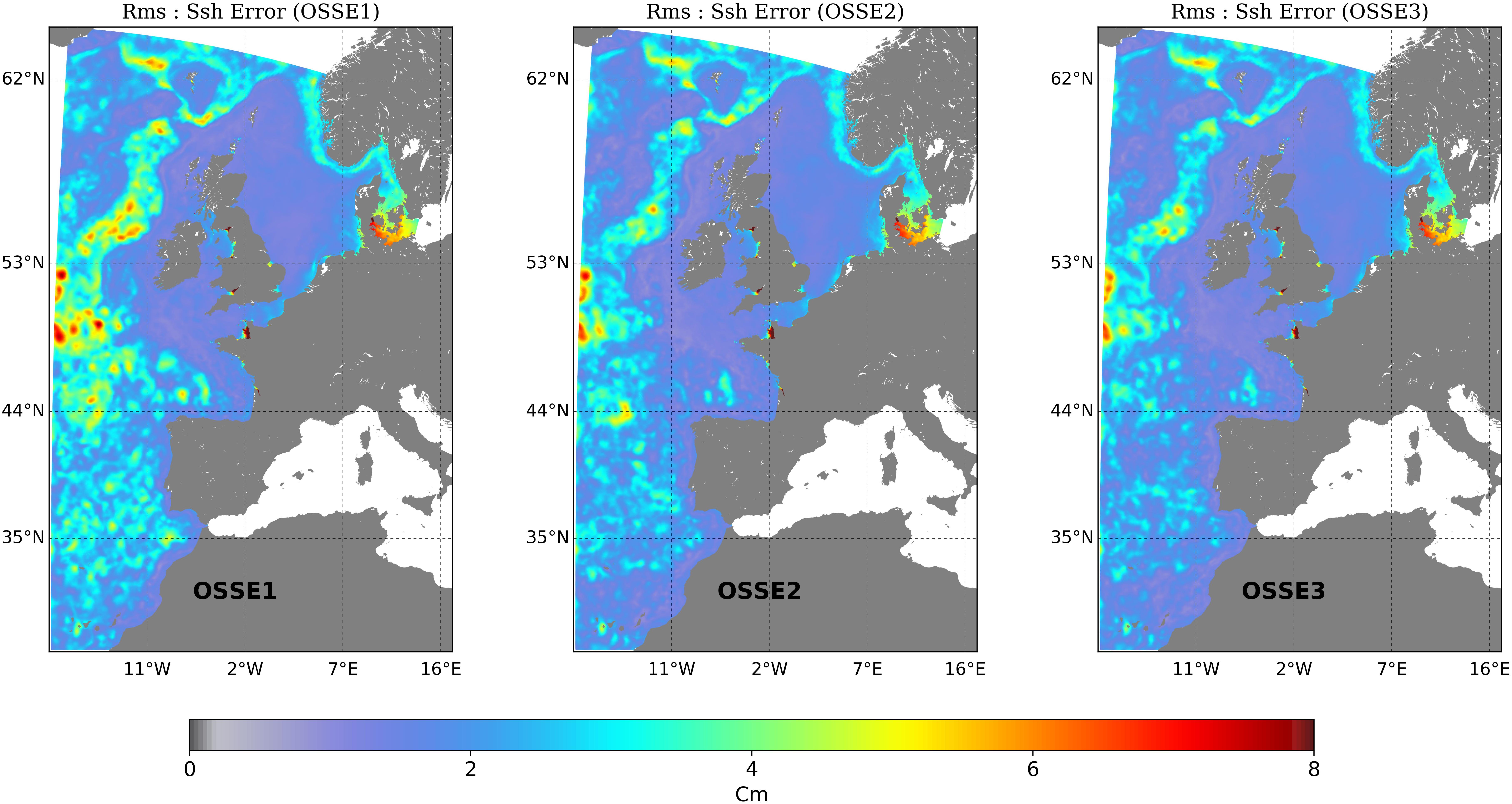
Figure 11. Map of the SSH analysis rms error over the IBI domain during 2009 (in cm). Results were obtained by comparing the analyzed SSH in the experiments OSSE1 (three nadir altimeters), OSSE2 (SWOT), and OSSE3 (SWOT + three nadir altimeters) with the data of the NatRun (Credits: Mercator Ocean).

Methods to deal with spatially correlated errors in SWOT [challenge (iv) above] have been developed by Ruggiero et al. (2016) and Yaremchuk et al. (2018). The common strategy consists of assimilating spatial derivatives of SWOT (along and across-track, first and second order) in addition to the original SWOT data itself. This is equivalent to assimilating SWOT data alone with a certain type of error correlation. The observation data set increases by a factor close to 5, but the assimilation can be performed assuming present-day assimilation tools. Ruggiero et al.’s (2016) study makes use of simulated SWOT data with degraded resolution; the next challenge is to move toward full resolution. Yaremchuk et al.’s (2018) method has not been tested yet in assimilation mode.

Fine-Scale SWOT 2D SSH and in situ Data for Observing 4D Ocean Dynamics

Surface Water and Ocean Topography will provide an exciting new view of the dynamic pressure field of the upper ocean, with unprecedented spatial resolution and coverage. This new window into ocean variability at wavelengths of 15–150 km will raise many new questions about ocean dynamics at these scales. Indeed, even the prospect of SWOT’s new measurements has stimulated many fundamental questions about the contributions of balanced and unbalanced dynamics to SSH variability (see section “Balanced and Unbalanced Motions”), the interpretation of SSH wavenumber spectra (see section SSH Wavenumber Spectra From Altimetry”), the small-scale structure of the marine geoid, approaches to in situ CalVal (see sections “SWOT Calibration and Validation on Wavenumber Spectrum,” “SWOT Validation Using in situ Observations,” and “The CalVal Site Near California”), and approaches to exploit the SWOT data to make inferences about the 3D flow field (see section “3D Projection From Surface Satellite SSH and SST/Density Observations”). Many of these questions are difficult to answer because they involve not only the 2D information that SWOT will provide, but also require more information than is currently available about the full spectrum of ocean variability in three spatial dimensions and time. In addition, the relationship between surface pressure fluctuations (SSH anomalies) and the many other dynamical quantities of interest (particularly horizontal and vertical velocity and property fluxes) is itself complicated at wavelengths below 150 km. SWOT data alone will not fully address the many pressing scientific questions concerning ocean variability at horizontal wavelengths below 150 km, but there are exciting opportunities to make advances on these questions by combining SWOT data with other measurements.

Over the last 25 years, many studies have analyzed the larger scale ocean dynamics using a combination of satellite altimetry and collocated in situ observations. Moorings have been aligned along altimetry groundtracks to study full-depth ocean transport and larger mesoscale variability, for example in the Kuroshio Current (Imawaki et al., 2001; Andres et al., 2008), across Drake Passage (Ferrari et al., 2013) or in the Agulhas Current (Beal et al., 2015). These moorings were generally spaced 1–2° apart, resolving only the larger-scale circulation. Gliders and ship-ADCP sections have been collocated with altimetric groundtracks (Heslop et al., 2017; Morrow et al., 2017), but these observations take days to cover hundreds of km, compared to altimetric observations in 30 s. In regions with rapidly moving dynamics, only small sections remain collocated. Dedicated in situ campaigns have provided insight at local sites into these rapidly evolving submesoscale dynamics at scales less than 15 km (e.g., OSMOSIS – Buckingham et al., 2016) or with campaigns that moved with energetic frontal features (e.g., LATMIX – Shcherbina et al., 2015). Specific campaigns have also investigated local internal wave dynamics (e.g., IWEX – Briscoe, 1975; Ocean Storms – D’Asaro et al., 1995), including with glider sections (Rainville et al., 2013). However, it remains a major observational challenge to resolve the 15–100 km ocean fine scales in time, depth, and the two horizontal dimensions, especially because internal tides and internal gravity waves require temporal sampling on the order of an 1 h.

A recent community workshop (held in Crystal City, VA, United States from 4 to 5 October 2018) focused on how the launch of SWOT and the activities occurring around it present opportunities for major advances in quantitative understanding of the dynamics of mesoscale, submesoscale, and internal-wave variability. The group of about 40 in-person and remote attendees discussed organizing one or more field campaigns, coordinated with SWOT satellite and cal/val measurements, to allow significant advances on the important science questions that motivated the SWOT mission. The NASA Sub-Mesoscale Ocean Dynamics Experiment (S-MODE) will include extensive measurements from aircraft, research vessels, and autonomous platforms in the SWOT CalVal region off of California during 2020–2021, and it presents another opportunity that can be leveraged toward a more complete understanding of the dynamics at scales below 150 km. By the end of the 2-day workshop, the group had identified a few important actions: (1) supporting the Adopt-a-Crossover effort being organized as a PI-driven effort to collect measurements in crossovers of the SWOT fast-repeat orbit, (2) organizing some additional measurements in the California Current region to complement the SWOT fast-repeat measurements, the SWOT CalVal array, and S-MODE measurements to make it possible to resolve the 4D ocean variability at a level of detail that has never been possible, and (3) to have a separate, dedicated SWOT field campaign in the Gulf Stream region 1–2 years after the SWOT launch. This third activity would have its primary scientific focus on the small mesoscales that SWOT would resolve, and it would take place during the ‘science orbit’ phase of SWOT (not the fast-repeat orbit) to allow the scientific community time to better assess and understand the SWOT data before trying to execute an in situ campaign intended to allow better use of the SWOT data.

Future, Forward Vision

Years before the SWOT launch, the promise of observing a new 2D SSH field over scales from 15 to 150 km is opening new research domains. Exciting questions are being explored on the role of small mesoscale and sub-mesoscale dynamics in the ocean circulation, and their impact on the energy budget, on mixing and dissipation, on the generation of larger-scale dynamics, and on the vertical exchange between the surface and deeper layers. Improving the horizontal and vertical flow at small scales should improve our understanding on the gateways of exchange of heat, freshwater, carbon, and nutrients across the oceans, and between the surface and deeper layers, with a big impact on biogeochemical cycles and biomass evolution.

Surface Water and Ocean Topography will be in a non-sun-synchronous orbit, specifically designed to provide our best 2D observation of the coastal and high-latitude tides, and the ocean’s internal tide field. This is a one-off opportunity – other planned wide swath missions for 2030+ are all on a sun-synchronous orbit, and will not resolve the full range of tidal constituents available with SWOT. This means that the SWOT era from 2022 to 2025 will be an exciting and unique opportunity to explore the role of internal tides and internal waves interacting with the “balanced” ocean circulation, and modifying the eddy energy, evolution and mixing on a global scale. Disentangling the balanced and unbalanced signals in SSH remains a challenge though, if we want to use SWOT or other fine-resolution alongtrack altimetry data to calculate balanced surface currents.

Mapping the fine-scale SWOT SSH swath data onto regular 2D fields presents many challenges, which are being explored using dynamical rather than statistical interpolation techniques, different vertical projection schemes, and full assimilation techniques. The improved small-scale sea surface height and surface currents from SWOT can also be analyzed in synergy with fine-scale satellite tracer data (SST, ocean color) and surface parameters (surface roughness, sun-glitter, etc.) that are strongly modified across fronts and filaments, in order to link the deeper dynamics with the surface fronts.

Finally, the altimetric mesoscale era was accompanied by a global Argo program that allowed us to collocate large-scale dynamics and eddies with vertical profiles. The question of how to collocate the rapidly evolving fine-scales observed by SWOT data with in situ data poses new challenges, that are actively being explored. Data mining of historical ADCP or glider data to re-analyze the high-frequency, fine-scales is one option. Developing new, rapid, fine-scale ocean profilers is another. Exploring the overlapping dynamics from small-scale ocean processes including internal waves and tides, using fine-resolution in situ and satellite data and models, will occupy a lot of our energy over the coming years.

Author Contributions

All authors contributed to write sections of the manuscript. All authors contributed to manuscript revision, read and approved the submitted version.

Funding

The authors were mostly funded through the NASA Physical Oceanography Program and the CNES/TOSCA programs for the SWOT and OSTST Science teams. AnP acknowledges support from the Spanish Research Agency and the European Regional Development Fund (Award No. CTM2016-78607-P). AuP acknowledges support from the ANR EQUINOx (ANR-17-CE01-0006-01).

Conflict of Interest Statement

The authors declare that the research was conducted in the absence of any commercial or financial relationships that could be construed as a potential conflict of interest.

Acknowledgments

The authors would like to acknowledge the work performed by the SWOT Science Team in the preparation of this mission. The authors thank D. Chelton and R. Samelson for careful reading and comments on the manuscript. The work of L-LF and JW was carried out at the Jet Propulsion Laboratory, California Institute of Technology, under a contract with the National Aeronautics and Space Administration (NASA).

References

Alpers, W. R. (1985). Theory of radar imaging of internal waves. Nature 314, 245–247. doi: 10.1038/314245a0

CrossRef Full Text | Google Scholar

Amores, A., Jordà, G., Arsouze, T., and Le Sommer, J. (2018). Up to what extent can we characterize ocean eddies using present day gridded altimetric products? J. Geophys. Res. Oceans 123, 7220–7236. doi: 10.1029/2018JC014140

CrossRef Full Text | Google Scholar

Andres, M., Park, J. H., Wimbush, M., Zhu, X. H., Chang, K. I., and Ichikawa, H. (2008). Study of the Kuroshio/Ryukyu current system based on satellite-altimeter and in situ measurements. Oceanogr. J. 64, 937–950. doi: 10.1007/s10872-008-0077-2

CrossRef Full Text | Google Scholar

Arbic, B. K., Alford, M. H., Ansong, J., Buijsman, M. C., Ciotti, R. B., Farrar, J. T., et al. (2018). “A primer on global internal tide and internal gravity wave continuum modeling in HYCOM and MITgcm,” in New Frontiers in Operational Oceanography, eds E. Chassignet, A. Pascual, J. Tintoré, and J. Verron (Mallorca: GODAE Ocean View).

Google Scholar

Ardhuin, F., Gille, S. T., Menemenlis, D., Rocha, C., Rascle, N., Chapron, B., et al. (2017). Small-scale open-ocean currents have large effects on ocean wave heights. J. Geophys. Res. Oceans 122, 4500–4517. doi: 10.1002/2016JC012413

CrossRef Full Text | Google Scholar

Auroux, D., and Blum, J. (2008). A nudging-based data assimilation method: the Back and Forth Nudging (BFN) algorithm. Nonlin. Process. Geophys. 15, 305–319. doi: 10.5194/npg-15-305-2008

CrossRef Full Text | Google Scholar

Barceló-Llull, B., Pascual, A., Mason, E., and Mulet, S. (2018). Comparing a multivariate global ocean state estimate with high-resolution in situ data: an anticyclonic intrathermocline eddy near the Canary Islands. Front. Mar. Sci. 5:66. doi: 10.3389/fmars.2018.00066

CrossRef Full Text | Google Scholar

Beal, L. M., Elipot, S., Houk, A., and Leber, G. M. (2015). Capturing the transport variability of a western boundary jet: results from the agulhas current time-series experiment (ACT). J. Phys. Oceanogr. 45, 1302–1324. doi: 10.1175/JPO-D-14-0119.1

CrossRef Full Text | Google Scholar

Bernstein, R., Breaker, L., and Whritner, R. (1977). California current eddy formation: ship, air, and satellite results. Science 195, 353–359. doi: 10.1126/science.195.4276.353

PubMed Abstract | CrossRef Full Text | Google Scholar

Blumen, W. (1978). Uniform potential vorticity flow: part I. Theory of wave interactions and two-dimensional turbulence. J. Atmos. Sci. 35, 774–783. doi: 10.1175/1520-0469(1978)035%3C0774%3Aupvfpi%3E2.0.co%3B2

CrossRef Full Text | Google Scholar

Brink, K. H., and Cowles, T. (1991). The coastal transition zone program. J. Geophys. Res. 96, 14637–14647.

Google Scholar

Briscoe, M. G. (1975). Preliminary results from the trimoored internal wave experiment (IWEX). J. Geophys. Res. 80, 3872–3884. doi: 10.1029/jc080i027p03872

CrossRef Full Text | Google Scholar

Buckingham, C. E., Naveira Garabato, A. C., Thompson, A. F., Brannigan, L., Lazar, A., Marshall, D. P., et al. (2016). Seasonality of submesoscale flows in the ocean surface boundary layer. Geophys. Res. Lett. 43, 2118–2126. doi: 10.1002/2016GL068009

CrossRef Full Text | Google Scholar

Bühler, O., Callies, J., and Ferrari, R. (2014). Wave–vortex decomposition of one-dimensional ship-track data. J. Fluid Mech. 756, 1007–1026. doi: 10.1017/jfm.2014.488

CrossRef Full Text | Google Scholar

Buongiorno Nardelli, B., Guinehut, S., Pascual, A., Drillet, Y., Ruiz, S., and Mulet, S. (2012). Towards high resolution mapping of 3-D mesoscale dynamics from observations. Ocean Sci. 8, 885–901. doi: 10.5194/os-8-885-2012

CrossRef Full Text | Google Scholar

Callies, J., and Ferrari, R. (2013). Interpreting energy and tracer spectra of upper-ocean turbulence in the submesoscale range (1–200 km). J. Phys. Oceanogr. 43, 2456–2474. doi: 10.1175/JPO-D-13-063.1

CrossRef Full Text | Google Scholar

Charney, J. G. (1971). Geostrophic turbulence. J. Atmos. Sci. 28, 1087–1095.

Google Scholar

Chassignet, E. P., and Xu, X. (2017). Impact of horizontal resolution (1/12° to 1/50°) on Gulf Stream separation, penetration, and variability. J. Phys. Oceanogr. 47, 1999–2021. doi: 10.1175/JPO-D-17-0031.1

CrossRef Full Text | Google Scholar

Chelton, D. B., Gaube, P., Schlax, M. G., Early, J. J., and Samelson, R. M. (2011). The influence of nonlinear mesoscale eddies on near-surface oceanic chlorophyll. Science 334, 328–332. doi: 10.1126/science.1208897

PubMed Abstract | CrossRef Full Text | Google Scholar

Chelton, D. B., Schlax, M. G., Samelson, R. M., Farrar, J. T., Molemaker, M. J., McWilliams, J. C., et al. (2019). Prospects for future satellite estimation of small-scale variability of ocean surface velocity and vorticity. Prog. Oceanogr. 173, 256–350. doi: 10.1016/j.pocean.2018.10.012

CrossRef Full Text | Google Scholar

Collard, F., Ardhuin, F., and Chapron, B. (2009). Monitoring and analysis of ocean swell fields using a spaceborne SAR: a new method for routine observations. J. Geophys. Res. 114:C07023. doi: 10.1029/2008JC005215

CrossRef Full Text | Google Scholar

Collins, C. A., Margolina, T., Rago, T. A., and Ivanov, L. (2013). Looping RAFOS floats in the California current system. Deep Sea Res. Part II Top. Stud. Oceanogr. 85, 42–61. doi: 10.1016/j.dsr2.2012.07.027

CrossRef Full Text | Google Scholar

D’Asaro, E. A., Eriksen, C. C., Levine, M. D., Paulson, C. A., Niiler, P., and Van Meurs, P. (1995). Upper-ocean inertial currents forced by a strong storm. Part I: data and comparisons with linear theory. J. Phys. Oceanogr. 25, 2909–2936. doi: 10.1175/1520-0485(1995)025%3C2909%3Auoicfb%3E2.0.co%3B2

CrossRef Full Text | Google Scholar

Desai, S. (2018). SWOT Project Science Requirements Document. California, CA: JPL Publication.

Google Scholar

Dibarboure, G., Pujol, M.-I., Briol, F., Le Traon, P. Y., Larnicol, G., Picot, N., et al. (2011). Jason-2 in DUACS: updated system description, first tandem results and impact on processing and products. Mar. Geod. 34, 214–241. doi: 10.1080/01490419.2011.584826

CrossRef Full Text | Google Scholar

Dong, C., McWilliams, J. C., Liu, Y., and Chen, D. (2014). Global heat and salt transports by eddy movement. Nat. Commun. 5:3294. doi: 10.1038/ncomms4294

PubMed Abstract | CrossRef Full Text | Google Scholar

Doodson, A. T. (1924). Meteorological perturbations of sea-level and tides. Geophys. J. Int. 1, 124–147. doi: 10.1073/pnas.1304912110

PubMed Abstract | CrossRef Full Text | Google Scholar

Dufau, C., Orsztynowicz, M., Dibarboure, G., Morrow, R., and Le Traon, P. Y. (2016). Mesoscale resolution capability of altimetry: present & future. J. Geophys. Res. Oceans 121, 4910–4927. doi: 10.1002/2015JC010904

CrossRef Full Text | Google Scholar

Dushaw, B. D., Worcester, P. F., and Dzieciuch, M. A. (2011). On the predictability of mode-1 internal tides. Deepn Sea Res. 58, 677–698. doi: 10.1016/j.dsr.2011.04.002

CrossRef Full Text | Google Scholar

Eldevik, T., and Dysthe, K. B. (2002). Spiral eddies. J. Phys. Oceanogr. 32, 851–869. doi: 10.1175/1520-0485(2002)032%3C0851%3Ase%3E2.0.co%3B2

PubMed Abstract | CrossRef Full Text | Google Scholar

Esteban-Fernandez, D. (2017). SWOT Mission Performance & Error Budget. California, CA: JPL Publication.

Google Scholar

Ferrari, R. (2011). Ocean science. A frontal challenge for climate models. Science 332, 316–317. doi: 10.1126/science.1203632

PubMed Abstract | CrossRef Full Text | Google Scholar

Ferrari, R., Provost, C., Sennechael, N., and Lee, J.-H. (2013). Circulation in drake passage revisited using new current time series and satellite altimetry: 2. The ona basin. J. Geophys. Res. Oceans 118, 147–165. doi: 10.1002/2012JC008193

CrossRef Full Text | Google Scholar

Ferrari, R., and Wunsch, C. (2009). Ocean circulation kinetic energy: reservoirs, sources, and sinks. Annu. Rev. Fluid Mech. 41, 253–282. doi: 10.1146/annurev.fluid.40.111406.102139

CrossRef Full Text | Google Scholar

Fresnay, S., Ponte, A. L., Le Gentil, S., and Le Sommer, J. (2018). Reconstruction of the 3D dynamics from surface variables in a high-resolution simulation of North Atlantic. J. Geophys. Res. Oceans 123, 1612–1630. doi: 10.1002/2017JC013400

CrossRef Full Text | Google Scholar

Fu, L.-L. (1983). On the wavenumber spectrum of oceanic mesoscale variability observed by the Seasat altimeter. J. Geophys. Res. 88, 4331–4341.

Google Scholar

Fu, L.-L., Alsdorf, D., Rodriguez, E., Morrow, R., Mognard, N., Lambin, J., et al. (2009). The SWOT (Surface Water and Ocean Topography) Mission: Spaceborne Radar Interferometry for Oceanographic and Hydrological Applications. .

Google Scholar

Fu, L. L., and Cazenave, A. (2001). Satellite Altimetry and Earth Sciences: A Handbook of Techniques and Applications. San Diego, CA: Academic Press.

Google Scholar

Fu, L. L., Rodriguez, E., Alsdorf, D., and Morrow, R. (eds) (2012). SWOT Mission Science document. California, CA: JPL Publication.

Google Scholar

Fu, L. L., and Ubelmann, C. (2014). On the transition from profile altimeter to swath altimeter for observing global ocean surface topography. J. Atmos. Ocean. Tech. 31, 560–568. doi: 10.1175/JTECH-D-13-00109.1

CrossRef Full Text | Google Scholar

Gómez-Navarro, L., Fablet, R., Mason, E., Pascual, A., Mourre, B., Cosme, E., et al. (2018). SWOT spatial scales in the western mediterranean sea derived from pseudo-observations and an Ad Hoc filtering. Remote Sens. 10:599. doi: 10.3390/rs10040599

CrossRef Full Text | Google Scholar

Guinehut, S., Dhomps, A., Larnicol, G., and Le Traon, P.-Y. (2012). High resolution 3D temperature and salinity fields derived from in situ and satellite observations. Ocean Sci. 8, 845–857. doi: 10.5194/os-8-845-2012

CrossRef Full Text | Google Scholar

Guinehut, S., Le Traon, P.-Y., and Larnicol, G. (2006). What can we learn from Global Altimetry/Hydrography comparisons? Geophys. Res. Lett. 33:L10604. doi: 10.1029/2005GL025551

CrossRef Full Text | Google Scholar

Heslop, E. E., Sánchez-Román, A., Pascual, A., Rodríguez, D., Reeve, K. A., Faugère, Y., et al. (2017). Sentinel-3A views ocean variability more accurately at finer resolution. Geophys. Res. Lett. 44:374. doi: 10.1002/2017GL076244

CrossRef Full Text | Google Scholar

Imawaki, S., Uchida, H., Ichikawa, H., Fukasawa, M., and Umatani, S. (2001). the ASUKA Group, Satellite altimeter monitoring the Kuroshio transport south of Japan. Geophys. Res. Lett. 28, 17–20. doi: 10.1029/2000gl011796

CrossRef Full Text | Google Scholar

Kahru, M., Mitchell, B. G., Gille, S. T., Hewes, C. D., and Holm-Hansen, O. (2007). Eddies enhance biological production in the Weddell-Scotia confluence of the Southern Ocean. Geophys. Res. Lett. 34:L14603. doi: 10.1029/2007GL030430

CrossRef Full Text | Google Scholar

Kelly, K. A., Dickinson, S., and Johnson, G. C. (2005). Comparisons of scatterometer and TAO winds reveal time-varying surface currents for the tropical pacific Ocean. J. Atmos. Ocean. Technol. 22, 735–745. doi: 10.1175/JTECH1738.1

CrossRef Full Text | Google Scholar

Kenyon, K. E. (1971). Wave refraction in ocean currents. Deep Sea Res. Oceanogr. Abstr. 18, 1023–1034. doi: 10.1016/0011-7471(71)90006-4

CrossRef Full Text | Google Scholar

Klein, P., Isern-Fontanet, J., Lapeyre, G., Roullet, G., Danioux, E., Chapron, B., et al. (2009). Diagnosis of vertical velocities in the upper ocean from high resolution sea surface height. Geophys. Res. Lett. 36:L12603. doi: 10.1029/2009GL038359

CrossRef Full Text | Google Scholar

Kudryavtsev, V., Akimov, D., Johannessen, J., and Chapron, B. (2005). On radar imaging of current features: 1. model and comparison with observations. J. Geophys. Res. 110:C07016. doi: 10.1029/2004JC002505

CrossRef Full Text | Google Scholar

Kudryavtsev, V., Kozlov, I., Chapron, B., and Johannessen, J. (2014). Quad-polarization SAR features of ocean currents. J. Geophy. Res. Oceans 119, 6046–6065. doi: 10.1002/2014JC010173

CrossRef Full Text | Google Scholar

Kudryavtsev, V., Myasoedov, A., Chapron, B., Johannessen, J. A., and Collard, F. (2012). Imaging mesoscale upper ocean dynamics using synthetic aperture radar and optical data. J. Geophys. Res. 117:C04029. doi: 10.1029/2011JC007492

CrossRef Full Text | Google Scholar

Kudryavtsev, V., Yurovskaya, M., Chapron, B., Collard, F., and Donlon, C. (2017). Sun glitter imagery of surface waves. Part 2: waves transformation on ocean currents. J. Geophys. Res. Oceans 122, 1384–1399. doi: 10.1002/2016JC012426

CrossRef Full Text | Google Scholar

Lapeyre, G. (2009). What vertical mode does the altimeter reflect? On the decomposition in baroclinic modes and on a surface-trapped mode. J. Phys. Oceanogr. 39, 2857–2874. doi: 10.1175/2009jpo3968.1

CrossRef Full Text | Google Scholar

Lapeyre, G., and Klein, P. (2006). Dynamics of the upper oceanic layers in terms of surface quasi-geostrophy theory. J. Phys. Oceanogr. 36, 165–176. doi: 10.1175/jpo2840.1

CrossRef Full Text | Google Scholar

Le Traon, P. Y., Klein, P., Hua, B. L., and Dibarboure, G. (2008). Do altimeter wavenumber spectra agree with the interior or surface quasi-geostrophic theory? J. Phys. Oceanogr. 38, 1137–1142. doi: 10.1175/2007JPO3806.1

CrossRef Full Text | Google Scholar

Le Traon, P. Y., Rouquet, M., and Boissier, C. (1990). Spatial scales of mesoscale variability in the North Atlantic as deduced from Geosat data. J. Geophys. Res. 95, 20267–20285. doi: 10.1029/JC095iC11p20267

CrossRef Full Text | Google Scholar

Lehahn, Y., d’Ovidio, F., and Koren, I. (2018). A satellite-based lagrangian view on phytoplankton dynamics. Ann. Review Mar. Sci. 10, 99–119. doi: 10.1146/annurev-marine-121916-063204

PubMed Abstract | CrossRef Full Text | Google Scholar

Lehahn, Y., Koren, I., Rudich, Y., Bidle, K. D., Trainic, M., Flores, J. M., et al. (2014). Decoupling atmospheric and oceanic factors affecting aerosol loading over a cluster of mesoscale North Atlantic eddies. Geophys. Res. Lett. 41, 4075–4081. doi: 10.1002/2014gl059738

CrossRef Full Text | Google Scholar

Lévy, M., Ferrari, R., Franks, P. J. P., Martin, A. P., and Riviere, P. (2012a). Bringing physics to life at the submesoscale. Geophys. Res. Lett. 39:L14602. doi: 10.1029/2012GL052756

CrossRef Full Text | Google Scholar

Lévy, M., Iovino, D., Resplandy, L., Klein, P., Madec, G., Treguier, A.-M., et al. (2012b). Large-scale impacts of sub-mesoscale dynamics on phytoplankton: local and remote effects. Ocean Modell. 43-44, 77–93. doi: 10.1016/j.ocemod.2011.12.003

CrossRef Full Text | Google Scholar

Lévy, M., Klein, P., and Treguier, A.-M. (2001). Impact of sub-mesoscale physics on production and subduction of phytoplankton in an oligotrophic regime. J. Mar. Res. 59, 535–565. doi: 10.1357/002224001762842181

CrossRef Full Text | Google Scholar

Lindborg, E. (2006). The energy cascade in a strongly stratified fluid. J. Fluid Mech. 550, 207–242.

Google Scholar

Liu, W. T., Katsaros, K. B., and Businger, J. A. (1979). Bulk parameterization of air–sea exchanges of heat and water vapor including the molecular constraints at the interface. J. Atmos. Sci. 36, 1722–1735. doi: 10.1175/1520-0469(1979)036%3C1722%3Abpoase%3E2.0.co%3B2

CrossRef Full Text | Google Scholar

Mahadevan, A. (2016). The impact of submesoscale physics on primary productivity of plankton. Ann. Rev. Mar. Sci. 8, 161–184. doi: 10.1146/annurev-marine-010814-015912

PubMed Abstract | CrossRef Full Text | Google Scholar

Manucharyan, G. E., and Thompson, A. F. (2017). Submesoscale Sea Ice-Ocean interactions in marginal ice zones. J. Geophys. Res. Oceans 122, 9455–9475. doi: 10.1002/2017JC012895

CrossRef Full Text | Google Scholar

Mason, E., Pascual, A., Gaube, P., Ruiz, S., Pelegrí, J. L., and Delepoulle, A. (2017). Subregional characterization of mesoscale eddies across the Brazil-malvinas confluence. J. Geophys. Res. Oceans 122, 3329–3357. doi: 10.1002/2016jc012611

CrossRef Full Text | Google Scholar

McWilliams, J., Colas, F., and Molemaker, M. (2009). Cold filamentary intensification and oceanic surface convergence lines. Geophys. Res. Lett. 36:L18602. doi: 10.1029/2009GL039402

CrossRef Full Text | Google Scholar

McWilliams, J. C. (2016). Submesoscale currents in the ocean. Proc. R. Soc. A 472:20160117. doi: 10.1098/rspa.2016.0117

PubMed Abstract | CrossRef Full Text | Google Scholar

Melville, W. K., Lenain, L., Cayan, D. R., Kahru, M., Kleissl, J. P., Linden, P. F., et al. (2016). The modular aerial sensing system. J. Atmos. Ocean. Technol. 33, 1169–1184. doi: 10.1175/JTECH-D-15-0067.1

CrossRef Full Text | Google Scholar

Morrow, R., Carret, A., Birol, F., Nino, F., Valladeau, G., Boy, F., et al. (2017). Observability of fine-scale ocean dynamics in the Northwest Mediterranean Sea. Ocean Sci. 13, 13–29. doi: 10.5194/os-13-13-2017

CrossRef Full Text | Google Scholar

Morrow, R., Blumstein, D., and Dibarboure, G. (2018a). “Fine-scale altimetry and the future SWOT mission,” in New Frontiers in Operational Oceanography, eds E. Chassignet, A. Pascual, J. Tintore, and J. Verron (Mallorca: GODAE Ocean View), 815. doi: 10.17125/gov2018

CrossRef Full Text | Google Scholar

Morrow, R., Fu, L.-L., Farrar, T., Seo, H., and Le Traon, P.-Y. (2018b). “Ocean eddies and mesoscale variability,” in Satellite Altimetry and Its Use for Earth Observation, eds D. Stammer and A. Cazenave (Boca Raton, FL: CRC Press).

Google Scholar

Mulet, S., Rio, M.-H., Mignot, A., Guinehut, S., and Morrow, R. (2012). A new estimate of the global 3D geostrophic ocean circulation based on satellite data and in-situ measurements. Deep Sea Res. Part II Top. Stud. Oceanogr. 77, 70–81. doi: 10.1016/j.dsr2.2012.04.012

CrossRef Full Text | Google Scholar

Munk, W. (1966). Abyssal recipes. Deep Sea Res. 13, 707–730. doi: 10.1016/0011-7471(66)90602-4

CrossRef Full Text | Google Scholar

Munk, W., Armi, L., Fischer, K., and Zachariasen, F. (2000). Spirals on the sea. Proc. R. Soc. Lond. 456, 1217–1280.

Google Scholar

Pascual, A., Ruiz, S., Buongiorno Nardelli, B., Guinehut, S., Iudicone, D., and Tintoré, J. (2015). Net primary production in the Gulf Stream sustained by quasi-geostrophic vertical exchanges. Geophys. Res. Lett. 42, 441–449. doi: 10.1002/2014GL062569

CrossRef Full Text | Google Scholar

Ponte, A., and Klein, P. (2013). Reconstruction of the upper ocean 3d dynamics from high resolution sea surface height. Ocean Dyn. 63, 777–791. doi: 10.1007/s10236-013-0611-7

CrossRef Full Text | Google Scholar

Ponte, A. L., and Klein, P. (2015). Incoherent signature of internal tides on seal level in idealized numerical simulations. Geophys. Res. Lett. 42, 1520–1526. doi: 10.1002/2014GL062583

CrossRef Full Text | Google Scholar

Ponte, A. L., Klein, P., Dunphy, M., and Gentil, S. L. (2017). Low-mode internal tides and balanced dynamics disentanglement in altimetric observations: synergy with surface density observations. J. Geophys. Res. Oceans 122, 2143–2155. doi: 10.1002/2016JC012214

CrossRef Full Text | Google Scholar

Qiu, B., Chen, S., Klein, P., Sasaki, H., and Sasai, Y. (2014). Seasonal mesoscale and submesoscale eddy variability along the North pacific subtropical countercurrent. J. Phys. Oceanogr. 44, 3079–3098. doi: 10.1175/jpo-d-14-0071.1

CrossRef Full Text | Google Scholar

Qiu, B., Chen, S., Klein, P., Ubelmann, C., Fu, L. L., and Sasaki, H. (2016). Reconstructability of 3-dimensional upper ocean circulation from SWOT sea surface height measurements. J. Phys. Oceanogr. 46, 947–963. doi: 10.1175/jpo-d-15-0188.1

CrossRef Full Text | Google Scholar

Qiu, B., Chen, S., Klein, P., Wang, J., Torres, H., Fu, L.-L., et al. (2018). Seasonality in transition scale from balanced to unbalanced motions in the world ocean. J. Phys. Oceanogr. 48, 591–605. doi: 10.1175/jpo-d-17-0169.1

CrossRef Full Text | Google Scholar

Qiu, B., Nakano, T., Chen, S., and Klein, P. (2017). Submesoscale transition from geostrophic flows to internal waves in the northwestern Pacific upper ocean. Nat. Commun. 8:14055. doi: 10.1038/ncomms14055

PubMed Abstract | CrossRef Full Text | Google Scholar

Quilfen, Y., Yurovskaya, M., Chapron, B., and Ardhuin, F. (2018). Storm waves sharpening in the Agulhas current: satellite observations and modeling. Remote Sens. Environ. 216, 561–571. doi: 10.1016/j.rse.2018.07.020

CrossRef Full Text | Google Scholar

Rainville, L., Lee, C. M., Rudnick, D. L., and Yang, K.-C. (2013). Propagation of internal tides generated near Luzon Strait: observations from autonomous gliders. J. Geophys. Res. Oceans 118, 4125–4138. doi: 10.1002/jgrc.20293

CrossRef Full Text | Google Scholar

Rascle, N., Molemaker, J., Marie, L., Nouguier, F., Chapron, B., Lund, B., et al. (2017). Intense deformation field at oceanic front inferred from directional sea surface roughness observations. Geophys. Res. Lett. 48, 5599–5608. doi: 10.1002/2017GL073473

CrossRef Full Text | Google Scholar

Rascle, N., Nouguier, F., Chapron, B., Mouche, A., and Ponte, A. (2016). Surface roughness changes by fine scale current gradients: properties at multiple azimuth view angles. J. Phys. Oceanogr. 46, 3681–3694. doi: 10.1175/JPO-D-15-0141.1

CrossRef Full Text | Google Scholar

Ray, R. D., and Zaron, E. D. (2016). M2 internal tides and their observed wavenumber spectra from satellite altimetry. J. Phys. Oceanogr. 46, 3–22. doi: 10.1175/JPO-D-15-0065.1

CrossRef Full Text | Google Scholar

Reid, J. (1961). On the geostrophic flow at the surface of the pacific ocean with respect to the 1,000-decibar Surface. Tellus 13, 489–502. doi: 10.3402/tellusa.v13i4.9520

CrossRef Full Text | Google Scholar

Renault, L., McWilliams, J. C., and Gula, J. (2018). Dampening of submesoscale currents by air-sea stress coupling in the californian upwelling System. Sci. Rep. 8:13388. doi: 10.1038/s41598-018-31602-3

PubMed Abstract | CrossRef Full Text | Google Scholar

Richman, J. G., Arbic, B. K., Shriver, J. F., Metzger, E. J., and Wallcraft, A. J. (2012). Inferring dynamics from the wavenumber spectra of an eddying global ocean model with embedded tides. J. Geophys. Res. 117:C12012. doi: 10.1029/2012JC008364

CrossRef Full Text | Google Scholar

Rio, M.-H., Santoleri, R., Bourdalle-Badie, R., Griffa, A., Piterbarg, L., and Taburet, G. (2016). Improving the altimeter-derived surface currents using high-resolution sea surface temperature data: a feasability study based on model outputs. J. Atmos. Ocean. Tech. 33, 2769–2784. doi: 10.1175/jtech-d-16-0017.1

CrossRef Full Text | Google Scholar

Rocha, C. S., Chereskin, T. K., Gille, S. T., and Menemenlis, D. (2016). Mesoscale to submesoscale wavenumber spectra in Drake Passage. J. Phys. Oceanogr. 46, 601–620. doi: 10.1175/JPO-D-15-0087.1

CrossRef Full Text | Google Scholar

Rodriguez, E., Esteban Fernandez, D., Peral, E., Chen, C. W., De Bleser, J.-W., and Williams, B. (2018). “Wide-swath altimetry: a review,” in Satellite Altimetry Over Oceans and Land Surfaces, Chap. 2, eds D. Stammer and A. Cazenave (Milton Park, NY: Taylor and Francis).

Google Scholar

Romero, L., Lenain, L., and Melville, W. K. (2017). Observations of surface wave–current interaction. J. Phys. Oceanogr. 47, 615–632. doi: 10.1175/JPO-D-16-0108.1

CrossRef Full Text | Google Scholar

Ruggiero, G. A., Cosme, E., Brankart, J.-M., Sommer, J. L., and Ubelmann, C. (2016). An efficient way to account for observation error correlations in the assimilation of data from the future SWOT high-resolution altimeter mission J. Atmos. Ocean. Technol. 33, 2755–2768. doi: 10.1175/jtech-d-16-0048.1

CrossRef Full Text | Google Scholar

Ruggiero, G. A., Ourmières, Y., Cosme, E., Blum, J., Auroux, D., and Verron, J. (2015). Data assimilation experiments using diffusive back-and-forth nudging for the NEMO ocean model. Nonlin. Process. Geophys. 22, 233–248. doi: 10.5194/npg-22-233-2015

CrossRef Full Text | Google Scholar

Ruiz, S., Pascual, A., Garau, B., Pujol, I., and Tintoré, J. (2009). Vertical motion in the upper oceanfrom glider and altimetry data. Geophys. Res. Lett. 36:L14607. doi: 10.1029/2009GL038569

CrossRef Full Text | Google Scholar

Sanchez de La Lama, M., LaCasce, J., and Fuhr, H. K. (2016). The vertical structure of ocean eddies. Dyn. Stat. Clim. Syst. 1:dzw001. doi: 10.1093/climsys/dzw001

CrossRef Full Text | Google Scholar

Sasaki, H., Klein, P., Qiu, B., and Sasai, Y. (2014). Impact of oceanic-scale interactions on the seasonal modulation of ocean dynamics by the atmosphere. Nat. Comm. 5, 1–8. doi: 10.1038/ncomms6636

PubMed Abstract | CrossRef Full Text | Google Scholar

Savage, A. C., Arbic, B. K., Alford, M. H., Ansong, J. K., Farrar, J. T., Menemenlis, D., et al. (2017). Spectral decomposition of internal gravity wave sea surface height in global models. J. Geophys. Res. 122, 7803–7821. doi: 10.1002/2017JC013009

CrossRef Full Text | Google Scholar

Shcherbina, A. Y., Sundermeyer, M. A., Kunze, E., D’Asaro, E., Badin, G., Birch, D., et al. (2015). The LatMix summer campaign: submesoscale stirring in the upper ocean. Bull. Amer. Meteor. Soc. 96, 1257–1279. doi: 10.1175/BAMS-D-14-00015.1

CrossRef Full Text | Google Scholar

Smith, K. S., and Vallis, G. K. (2001). The scales and equilibration of mid-ocean eddies: freely evolving flow. J. Phys. Oceanogr. 31, 554–571. doi: 10.1175/1520-0485(2001)031%3C0554%3Atsaeom%3E2.0.co%3B2

CrossRef Full Text | Google Scholar

Stammer, D. (1997). Global characteristics of ocean variability estimated from regional TOPEX/POSEIDON altimeter measurements. J. Phys. Oceanogr. 27, 1743–1769. doi: 10.1175/1520-0485(1997)027<1743:GCOOVE>2.0.CO;2

CrossRef Full Text | Google Scholar

Stammer, D., Ray, R. D., Andersen, O. B., Arbic, B. K., Bosch, W., Carrere, L., et al. (2014). Accuracy assessment of global barotropic ocean tide models. Rev. Geophys. 52, 243–282. doi: 10.1002/2014RG000450

CrossRef Full Text | Google Scholar

Sverdrup, H. U., and Fleming, R. H. (1941). The waters off the coast of southern California, March to July, 1937. Bull. Scripps Inst. Oceanogr. 4, 261–378.

Google Scholar

Tchilibou, M., Gourdeau, L., Morrow, R., Serazin, G., Djath, B., and Lyard, F. (2018). Spectral signatures of the tropical Pacific dynamics from model and altimetry: a focus on the meso-submesoscale range. Ocean Sci. 14, 1283–1301. doi: 10.5194/os-14-1283-2018

CrossRef Full Text | Google Scholar

Ubelmann, C., Cornuelle, B., and Fu, L. (2016). Dynamic mapping of along-track ocean altimetry: method and performance from observing system simulation experiments. J. Atmos. Ocean. Technol. 33, 1691–1699. doi: 10.1175/JTECH-D-15-0163.1

CrossRef Full Text | Google Scholar

Ubelmann, C., Dibarboure, G., and Dubois, P. (2018). A cross-spectral approach to measure the error budget of the SWOT altimetry mission over the Ocean. J. Atmos. Ocean. Technol. 35, 845–857. doi: 10.1175/JTECH-D-17-0061.1

CrossRef Full Text | Google Scholar

Ubelmann, C., Klein, P., and Fu, L.-L. (2015). Dynamic interpolation of sea surface height and potential applications for future high-resolution altimetry mapping. J. Atmos. Ocean. Technol. 32, 177–184. doi: 10.1175/jtech-d-14-00152.1

CrossRef Full Text | Google Scholar

Vergara, O., Morrow, R., Pujol, I., Dibarboure, G., and Ubelmann, C. (2019). Revised global wavenumber spectra from recent altimeter observations. J. Geophys. Res. doi: 10.1029/2018JC014844

CrossRef Full Text | Google Scholar

Wang, J., Flierl, G., LaCasce, J., McClean, J., and Mahadevan, A. (2013). Reconstructing the ocean’s interior from surface data. J. Phys. Oceanogr. 43, 1611–1626. doi: 10.1175/jpo-d-12-0204.1

CrossRef Full Text | Google Scholar

Wang, J., Fu, L., Qiu, B., Menemenlis, D., Farrar, J. T., Chao, Y., et al. (2018). An observing system simulation experiment for the calibration and validation of the surface water ocean topography sea surface height measurement using in situ platforms. J. Atmos. Ocean. Technol. 35, 281–297. doi: 10.1175/JTECH-D-17-0076.1

CrossRef Full Text | Google Scholar

Wang, J., and Fu, L. L. (2019). On the long-wavelength validation of the SWOT KaRIn measurement. J. Atmos. Ocean. Tech. doi: 10.1175/JTECH-D-18-0148.1 [Epub ahead of print].

CrossRef Full Text | Google Scholar

Wang, J., Fu, L. L., Torres, H. S., Chen, S., Qiu, B., and Menemenlis, D. (2019). On the spatial scales to be resolved by the surface water and ocean topography Ka-band radar interferometer. J. Atmos. Ocean. Tech. 36, 87–99. doi: 10.1175/JTECH-D-18-0119.1

CrossRef Full Text | Google Scholar

Wunsch, C. (1997). The vertical partition of oceanic horizontal kinetic energy. J. Phys. Oceanogr. 27, 1770–1794. doi: 10.1175/1520-0485(1997)027%3C1770%3Atvpooh%3E2.0.co%3B2

CrossRef Full Text | Google Scholar

Wyllie, J. G. (1966). Geostrophic flow of the California Current at the surface and at 200 meters. Calif. Coop. Ocean. Fish. Invest. Atlas 4:531.

Google Scholar

Xu, Y., and Fu, L.-L. (2011). Global variability of the wavenumber spectrum of oceanic mesoscale turbulence. J. Phys. Oceanogr. 41, 802–809. doi: 10.1175/2010JPO4558.1

CrossRef Full Text | Google Scholar

Xu, Y., and Fu, L.-L. (2012). The effects of altimeter instrument noise on the estimation of the wavenumber spectrum of sea surface height. J. Phys. Oceanogr. 42, 2229–2233. doi: 10.1175/JPO-D-12-0106.1

CrossRef Full Text | Google Scholar

Yaremchuk, M., D’Addezio, J., Panteleev, G., and Jacobs, G. (2018). On the approximation of the inverse error covariances of high resolution satellite altimetry data. Quart. J. R. Meteor. Soc. 144, 1995–2000. doi: 10.1002/qj.3336

CrossRef Full Text | Google Scholar

Yoder, J. A., Ackleson, S. G., Barber, R. T., Flament, P. F., and Balch, W. M. (1994). A line in the sea. Nature 371, 689–692.

Google Scholar

Zaron, E. D., and Ray, R. D. (2017). Using an altimeter-derived internal tide model to remove tides from in-situ data. Geophys. Res. Lett. 44, 1–5. doi: 10.1002/2017GL072950

CrossRef Full Text | Google Scholar

Zhao, Z., Alford, M. H., Girton, J. B., Rainville, L., and Simmons, H. L. (2016). Global observations of open-ocean mode-1 M2 internal tides. J. Phys. Oceanogr. 46, 1657–1684. doi: 10.1175/JPO-D-15-0105.1

CrossRef Full Text | Google Scholar