Air-Sea Heat Flux Variability in the Southeast Indian Ocean and Its Relation With Ningaloo Niño

Introduction

The southeast Indian Ocean (IO) is a region where extreme climate variability and a unique ocean circulation are observed. During 2010–2011, an extreme marine heat wave associated with ocean warming occurred off the west coast of Australia. This extreme warming event is termed as “Ningaloo Niño” (Feng et al., 2013). The 2010–2011 Ningaloo Niño event was associated with anomalous ocean circulations in the southeast IO. For example, there was an unseasonable surge of the Leeuwin Current, which flows southward against prevailing southerly winds along the west coast of Australia, bringing warm waters from the tropics. These extreme oceanic conditions have a substantial impact on marine ecosystem and regional climate variability (Pearce and Feng, 2013; Wernberg et al., 2013; Caputi et al., 2014; Kataoka et al., 2014; Tozuka et al., 2014).

In the southeast IO near the west coast of Australia, relatively large annual mean surface heat fluxes (cooling the ocean) with the strong seasonal cycle are observed (Feng et al., 2003, 2008). For the annual mean, a large amount of heat loss of the ocean occurs at the air-sea interface in a broad area off the west coast of Australia. The majority of the heat loss is caused by a large evaporative cooling due to warm SSTs in the region of the Leeuwin Current. The annual cycle of net surface heat flux is dominated by shortwave radiation and latent heat flux. During the austral winter, shortwave radiation is weak, but the latent heat flux (cooling) is large due to a stronger Leeuwin Current (and thus warm SSTs) and low near-surface specific humidity associated with the cold air temperature. During the austral summer, shortwave radiation is strong, and the latent heat flux is small due to a weaker Leeuwin Current (Feng et al., 2003, 2008) and higher near-surface specific humidity associated with the warmer air temperature.

In addition to the strong seasonal cycle of air-sea heat fluxes, significant interannual variations of surface heat fluxes are found in this region including those associated with the Ningaloo Niño. Some of the previous studies suggest that the SST warming during the Ningaloo Niño is caused by the heat advection by the strengthening of the Leeuwin Current especially for the 2010–2011 event, whereas air-sea heat fluxes also contribute to the warming (Feng et al., 2013; Zhang et al., 2018). However, the relative importance of heat advection by the Leeuwin Current and surface heat fluxes on the development of the Ningaloo Niño varies substantially between different studies. For example, Benthuysen et al. (2014) indicated that reduced latent and sensible heat fluxes around the peak phase account for 1/3 of the warming during the 2010/2011 event in addition to the heat advection produced by the strengthening of Leeuwin Current. On the other hand, a composite analysis of multiple Ningaloo Niño events indicated that the initial offshore warming is primarily caused by the anomalous latent heat flux (Marshall et al., 2015). Kataoka et al. (2014) classified the Ningaloo Niño to locally and non-locally amplified modes based on the local wind anomalies and suggested that the reduction of latent heat flux enhances offshore warming during the development and coastal warming during the peak in both modes. Recently, Kataoka et al. (2017) calculated the mixed layer temperature balance associated with Ningaloo Niño events and found that shortwave radiation contributes to the coastal warming in both locally and non-locally amplified modes due to the warming produced by the climatological surface heat flux enhanced by the shallow mixed-layer depth (MLD) anomaly during the onset. Moreover, Xu et al. (2018) compared the difference in SST warming patterns between the 2012/2013 event with the 2010/2011 event and found that the difference in the relative importance of surface heat fluxes and heat advection between the two events is mostly responsible for the different spatial distribution of the warming.

As described above, a variety of different conclusions on the role of surface heat fluxes in the warming during the Ningaloo Niño have been obtained in previous studies. These differences could partly be due to the different source of surface flux datasets, which include various satellite observations, reanalysis products, and model simulations. The systematic analysis of air-sea heat flux variability associated with the Ningaloo Niño using multiple datasets is thus necessary to reconcile previous studies and determine the uncertainties on the role of air-sea fluxes.

While most of the previous studies focus on processes during the onset and development (warming period) of the Ningaloo Niño, processes that control the cooling during the recovery phase have received little attention. A recent study by Kataoka et al. (2017) discussed processes during both the development and demise of the Ningaloo Niño and suggested that the mixed layer temperature is influenced by not only heat flux anomalies but also MLD anomalies which change the heat capacity. They concluded that the net effect of latent heat flux is not as important as earlier studies suggested during the recovery phase because of the anomalously deep mixed layers and thus a large heat capacity. In addition, the significant role of sensible heat flux for the locally-amplified mode is suggested. However, these conclusions are based on the analysis of a single numerical model simulation and it is possible that different results could be obtained using different datasets. Accordingly, it is necessary to examine the processes during the recovery phase using multiple datasets, and such analyses will provide better insights into the role of air-sea fluxes during the recovery phase.

In addition to the large influence of surface heat fluxes on SST and upper ocean during the Ningaloo Niño, air-sea heat fluxes influence the atmospheric conditions and the large-scale atmospheric circulations, and in turn they can feedback on SSTs. Various feedback mechanisms between the atmosphere and ocean associated with the Ningaloo Niño have been suggested in recent years. For example, Tozuka and Oettli (2018) showed that during the Ningaloo Niño, positive SST anomalies increase the formation of cloud and thus decrease the shortwave radiation, which will weaken the initial warming. Zhang and Han (2018) found that SST anomalies in the southeast IO associated with the Ningaloo Niño lead to the enhancement of western Pacific trade winds and the cooling in the central Pacific. The enhanced trade winds could strengthen the ITF and the cooling anomalies in the central Pacific could induce cyclonic wind anomalies in the southeast IO, both of which will amplify the initial warming of Ningaloo Niño. As changes in air-sea fluxes in the southeast IO are essential components of these feedback mechanisms, assessing the uncertainties of surface fluxes using multiple datasets is necessary for further exploring these air-sea interaction processes.

The uncertainties of air-sea heat fluxes arise from the errors in bulk atmospheric variables and SST, which are derived from reanalysis products and satellite observations, and use of different bulk flux algorithms (Brunke et al., 2002; Wu et al., 2006; Kubota et al., 2008; Valdivieso et al., 2017). In the area off the west coast of Australia, the uncertainties and thus the difference between the datasets could be very large because of the large variability of SST and associated atmospheric variables caused by Leeuwin Current variations. Hence thorough description of air-sea fluxes in this region using multiple datasets and their comparisons are crucial for the investigation of climate variability in this region including the Ningaloo Niño.

The purpose of this study is to investigate the air-sea heat fluxes associated with the development and decay of Ningaloo Niño and to identify the major sources of uncertainties in the interannual variability using multiple datasets. In particular, the air-sea heat flux variations during the decay phase of the Ningaloo Niño is emphasized. The rest of this paper is organized as follows. Section “Materials and Methods” describes the data and method used in this study. In Section “Results”, climatological air-sea fluxes from different datasets are compared, and the effect of latent heat flux variability on the Ningaloo Niño is studied based on the composite analysis. A discussion and summary are presented in Sections “Discussion and Summary.”

TABLE 1

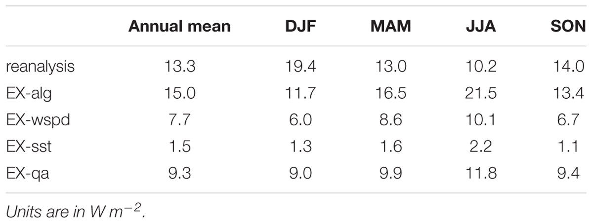
Table 1. Mean absolute deviation of annual and seasonal mean latent heat flux calculated from reanalysis, EX-alg, EX-wspd, EX-sst, and EX-qa.

Data and Methods

Reanalysis

Daily short and longwave radiation, and latent and sensible heat fluxes from five major reanalysis products are used in this study. These are the National Center for Environmental Prediction-National Centers for Atmospheric Research (NCEP/NCAR) reanalysis-1 (NCEP1; Kalnay et al., 1996), the NCEP-Department of Energy (NCEP/DOE) reanalysis (NCEP2; Kanamitsu et al., 2002), the European Centre for Medium-Range Weather Forecasts (ECMWF) Interim reanalysis (ERA-Interim; Dee et al., 2011), NASA’s Modern-Era Retrospective analysis for Research and Applications, Version 2 reanalysis (MERRA-2; Gelaro et al., 2017), and NCEP Climate Forecast System Reanalysis (CFSR; Saha et al., 2010, 2014). NCEP1 and NCEP2 are available on the T62 Gaussian grid with a spatial resolution of about 1.875° × 1.875°. CFSR reanalysis is based on a coupled ocean-atmosphere-land data assimilation system that consists of an atmospheric component at a resolution of T382 (38 km) and an ocean component at a resolution of 0.5° beyond the tropics. ERA-Interim data is on 0.75° × 0.75° grid, and MERRA2 uses an approximate resolution of 0.5° × 0.625°. The data for the period 1985–2016 is analyzed during which all these datasets are available. To investigate the effect of MLD variation on SSTs (Kataoka et al., 2017), MLD obtained from 1/12° Hybrid Coordinate Ocean Model (HYCOM) reanalysis (Metzger et al., 2014) for 1994–2015 is used.

OAFlux

We also used daily gridded (1° × 1°) bulk flux state variables (i.e., wind speed, air and sea surface temperature, and humidity) from WHOI Objectively Analyzed Ocean-Atmosphere Flux (OAFlux) product (Yu et al., 2008) to calculate the latent heat flux using the state-of-the-art COARE3.5 bulk algorithm (Fairall et al., 2003). The state variables provided by OAFlux blended observational and reanalysis data from various sources based on an objective analysis to obtain an optimal estimate of the atmospheric and oceanic conditions. The daily state variables for the period 1985–2016 are used in the analysis. The latent heat flux estimates calculated here are well correlated with those from the gridded flux provided by OAFlux (r = 0.997) but have a Root Mean Square error (RMSE) of 7.8 W m^-2. This difference is primarily caused by the lack of SST correction associated with the cool skin and warm layer in our calculation, and the difference due to the use of different versions of bulk formula (COARE3.5 and COARE3.0) is very small (RMSE:0.6 W m^-2). Note that the RMSE between latent heat flux estimates using COARE3.5 and those provided by OAFlux is much smaller (2.1 W m^-2) during DJF when Ningaloo Niño develops, and thus the effect of the cool skin and warm layer is very small during this season.

Satellite and Buoy Observations

Monthly satellite-derived radiation fluxes from Clouds and Earth’s Radiant Energy Systems (CERES; Kato et al., 2018) for the period 2000–2016 are used. Surface fluxes and bulk flux state variables from the Research Moored Array for African-Asian-Australian Monsoon Analysis and Prediction (RAMA) at 25°S, 100°E (McPhaden et al., 2009) from September 2012 to 2014 are also used for the comparison with gridded flux data products. The surface air-sea fluxes were estimated using COARE3.0b.

Besides flux datasets, we also use daily high resolution SST products obtained from National Oceanic and Atmospheric Administration (NOAA) Optimum Interpolation Sea Surface Temperature based on Advanced Very High Resolution Radiometer (AVHRR) observations (OISST; Reynolds et al., 2007.;Banzon et al., 2016; 0.25° × 0.25°; 1985–2016) and Multi-scale Ultra-high Resolution (MUR) Sea Surface Temperature (SST) analysis produced at Jet Propulsion Laboratory (Chin et al., 2017.; 0.01° × 0.01°; 2002–2016).

Results

Climatology

Before examining the air-sea flux variations associated with the Ningaloo Niño, climatological air-sea fluxes in this region and their uncertainties are investigated by comparing those from different datasets (Figure 1A and Table 1). The seasonal cycle of latent heat flux from all products are similar, in which large (small) latent heat release in the austral winter (summer) is found. However, remarkable quantitative differences are found especially in summer (Figure 1A), during which the maximum difference can be as large as ∼80 W m^-2.

FIGURE 1

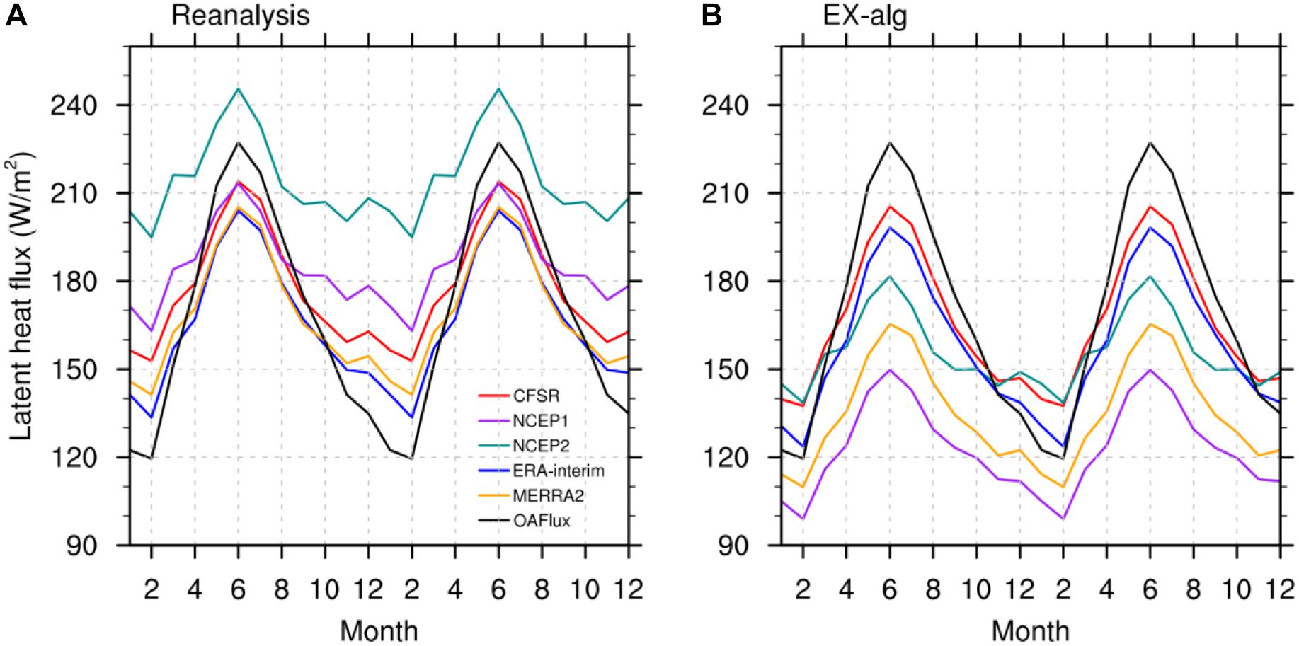
Figure 1. Climatological seasonal cycle of latent heat flux calculated for the area around the west coast of Australia (110°E-116°E, 22°S-32°S) from (A) reanalysis products, (B) sensitivity calculations using COARE3.5 algorithm (EX-alg). Positive values indicate the flux from the ocean to the atmosphere.

To further quantify the uncertainties, mean absolute deviation (MAD) defined as $\mathit{M}\mathit{A}\mathit{D}\mathrm{=}\frac{{\mathrm{\Sigma }}_{\mathit{i}\mathrm{=}\mathrm{1}}^{\mathit{n}}\mathrm{|}{\mathit{X}}_{\mathit{i}}\mathrm{-}\overline{\mathit{X}}\mathrm{|}}{\mathit{n}}$, where X_i is surface heat flux from reanalysis, $\overline{\mathit{X}}$ is the mean value of all datasets, and n is the number of datasets, is calculated (Table 1, first row). Since MAD measures the magnitude of inter-data spread, the difference in uncertainties between the datasets could be determined quantitatively by calculating MAD. While large uncertainties are found in all seasons, the uncertainty is particularly large during summer with the MAD of 19.4 W m^-2 when the difference between the highest and lowest latent heat flux exceeds 80 W m^-2.

Uncertainties of latent heat fluxes could partly be due to the use of different bulk flux algorithms. To evaluate the uncertainties caused by the use of different bulk flux algorithms, we recalculated the daily latent heat flux by using COARE3.5 flux algorithm and the state variables from each reanalysis product (referred to as EX-alg, where “EX” and “alg” stand for “experiment” and “algorithm”). Figure 1B show the climatological seasonal cycle of latent heat flux from EX-alg. The difference between the values in Figures 1A,B is a measure of uncertainty caused by the use of different algorithms. Based on the comparison, the algorithms used in reanalysis products tend to produce higher values than COARE3.5. For example, the difference is ∼60 W m^-2 for NCEP1 and NCEP2, ∼30 W m^-2 for MERRA2, and ∼10 W m^-2 for ERA-Interim and CFSR. Higher values of latent heat flux in reanalysis data have been documented in previous studies at various locations (e.g., Kubota et al., 2008; Zhang et al., 2016). For example, Kubota et al. (2008) evaluated the latent heat flux from NCEP1 and NCEP2 by comparing with the measurement at the Kuroshio Extension Observatory site. Both datasets overestimated the latent heat flux with a bias of 41 and 62 W m^-2. They suggest that this bias is primarily caused by the use of different algorithms. The major difference between bulk flux algorithms is how the transfer coefficients vary with wind speeds, atmospheric stability and other physical processes that influence the transfer of heat and moisture at the sea surface. Yet further details why the algorithms used in reanalysis tends to produce higher values are still unknown. The MAD of algorithm-caused uncertainty is 21.3, 25.0, 26.0, and 22.5 W m^-2 during DJF, MAM, JJA and SON, respectively, showing a weak seasonal variation. This is because the uncertainty depends on both the magnitude of latent heat flux (larger in winter) and wind speed (smaller in winter). Further details of the seasonal dependence are discussed in the Appendix.

The shortwave radiation also reveals a strong seasonal variation (Figure 2B). Similar to latent heat flux, large uncertainties are found in summer. Assuming the satellite derived estimate (CERES) is more accurate than reanalysis products, the estimate of NCEP1 has the largest bias (∼80 W m^-2) in summer, and estimates in other datasets have smaller biases of ∼20 W m^-2. Shortwave radiation and latent heat flux are dominant components of the seasonal variations of net surface heat flux. Considerable net surface heat flux differences between the datasets are found during summer when the Ningaloo Niño develops (Figure 2A). Most of the differences arise from latent heat flux and shortwave radiation as discussed above. The contribution of the difference in longwave radiation and sensible heat flux between the different datasets is minimal.

FIGURE 2

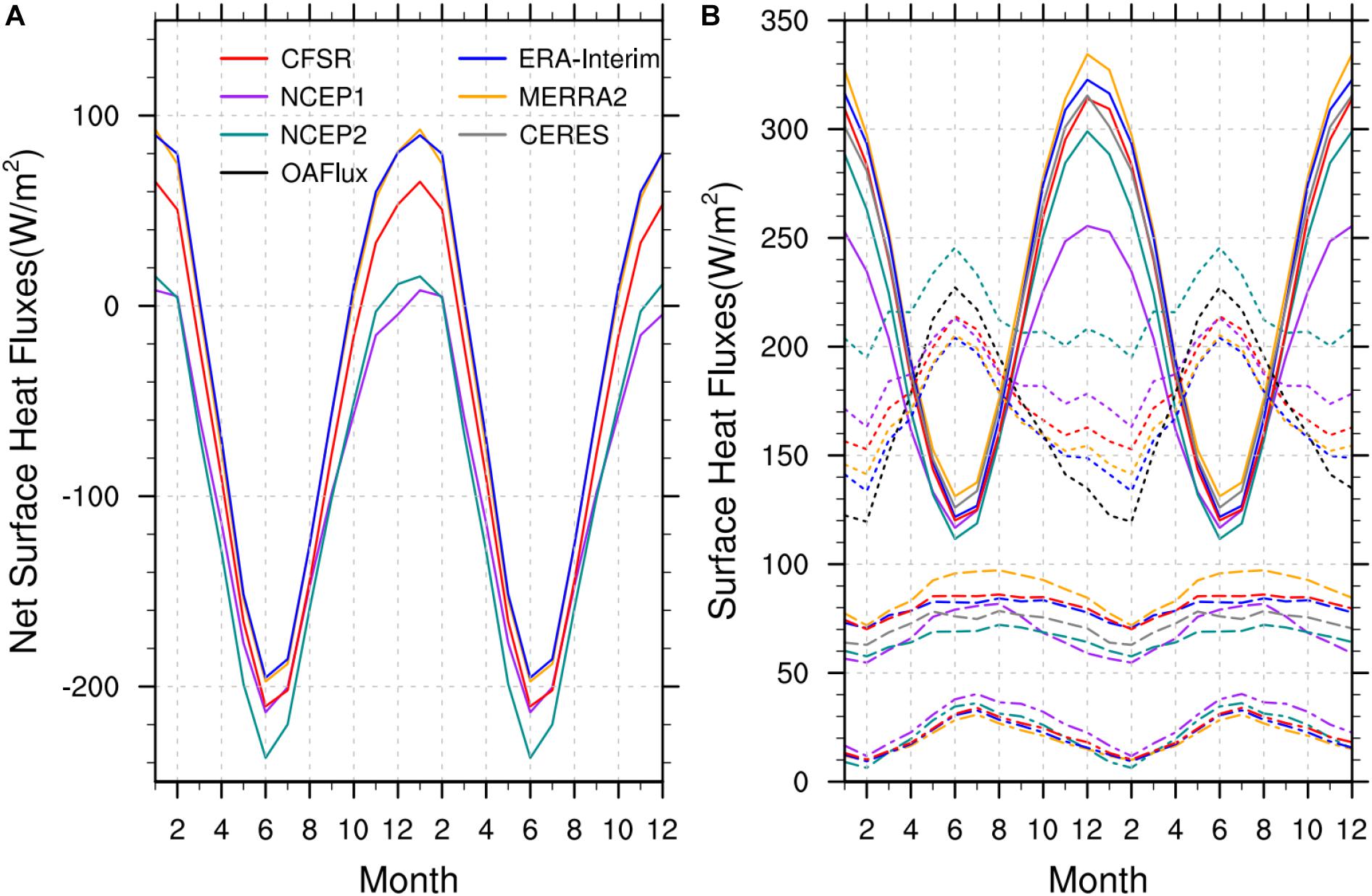
Figure 2. (A) Climatological seasonal cycle of the net surface heat flux calculated for the area around the west coast of Australia (110°E-116°E, 22°S-32°S). (B) Same as in (A), but for net shortwave radiation (solid line), net longwave radiation (dashed line), latent heat flux (dotted line) and sensible heat flux (dot-dashed line). Colors indicate different datasets. Positive values indicate the flux into the ocean (atmosphere) for net surface heat flux and shortwave radiation (longwave radiation, latent and sensible heat flux).

Figure 3 compares the monthly surface heat flux from reanalysis products with the RAMA buoy at 100°E, 25°S for the 2-year period during which buoy measurements are available. The variations of latent heat flux from OAFlux and shortwave radiation from CERES agree well with those from the RAMA buoy. Large differences in shortwave radiation between the datasets are found during the austral summer. Both NCEP1 and CFSR greatly underestimate the net shortwave radiation. The seasonal variations of latent and sensible heat flux at the buoy site are weaker, and the mean value is smaller than those near the west coast of Australia due to the weaker influence of the Leeuwin Current at this location. An overestimate of 10–50 W m^-2 in latent heat flux from reanalysis products is found throughout the analysis period, suggesting that these differences are partly due to the use of different bulk flux algorithms. The use of COARE3.5 improves the latent heat flux for most of the datasets (Figure 4A). MAD decreases from 11.5 to 7.5 W m^-2 for CFSR, 25.3 to 13.7 W m^-2 for NCEP2, 24.7 to 23.4 W m^-2 for ERA-Interim and 15.9 to 13.2 W m^-2 for MERRA2, but it increases from 17.7 to 28.2 W m^-2 for NCEP1 due to large errors in the specific humidity and wind speed (Figures 4B,C).

FIGURE 3

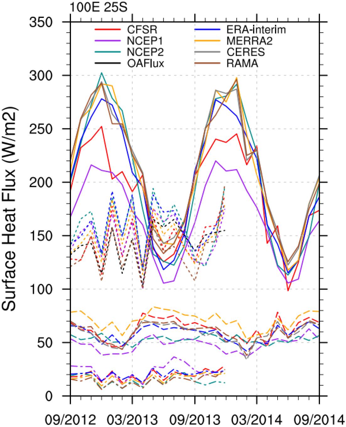
Figure 3. Comparison of monthly mean surface heat fluxes from reanalysis products with those from RAMA buoy observations at 100°E, 25°S: net shortwave radiation (solid line), net longwave radiation (dashed line), latent heat flux (dotted line) and sensible heat flux (dot-dashed line). Positive values indicate the flux into the ocean (atmosphere) for shortwave radiation (longwave radiation, latent and sensible heat flux).

FIGURE 4

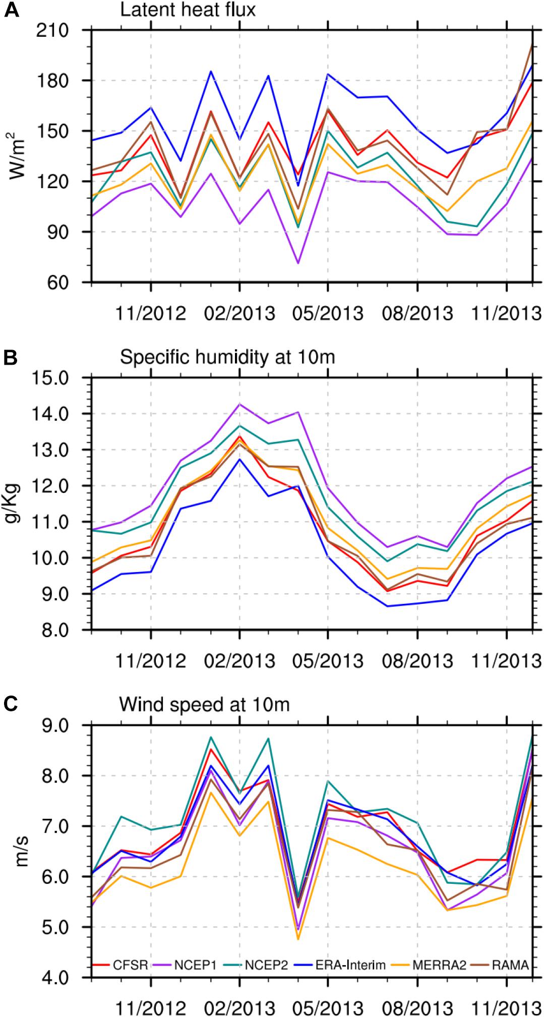
Figure 4. (A) Comparison of monthly mean latent heat flux from EX-alg with those from the RAMA buoy at 100°E, 25°S. The positive values indicate the flux from the ocean to the atmosphere. (B) Comparison of Specific humidity at 10 m from reanalysis with those from RAMA buoy at the same location. (C) Same as in (B), but for wind speed at 10 m.

While the use of different bulk flux algorithms causes significant difference in estimated fluxes, large differences still exist when using the same algorithm (Figures 1B, 4A), indicating that the difference in bulk variables largely influences the estimates of latent heat flux. To evaluate the uncertainties caused by each bulk variable, we calculated the daily latent heat flux using COARE3.5 for three different cases, in which bulk variables are (1) surface wind speed only from each reanalysis and other variables from OAFlux (EX-wspd), (2) SST only from each reanalysis and other variables from OAFlux (EX-sst), (3) air humidity only from each reanalysis and other variables from OAFlux (EX-qa). The uncertainties caused only by windspeed, SST and air humidity can be estimated from EX-wspd, EX-sst, and EX-qa, respectively. Both surface wind speed and humidity largely contribute to the difference between the datasets, whereas the contribution of SST is much smaller (Figure 5). The MAD of annual mean latent flux is 7.7 and 9.3 W m^-2 for EX-wspd and EX-qa, and that of EX-sst is 1.5 W m^-2 (Table 1). All latent heat fluxes calculated with reanalysis state variables are underestimated in EX-wspd and EX-qa during winter, but not during summer. The MAD during winter is also larger than in summer in EX-wspd and EX-qa.

FIGURE 5

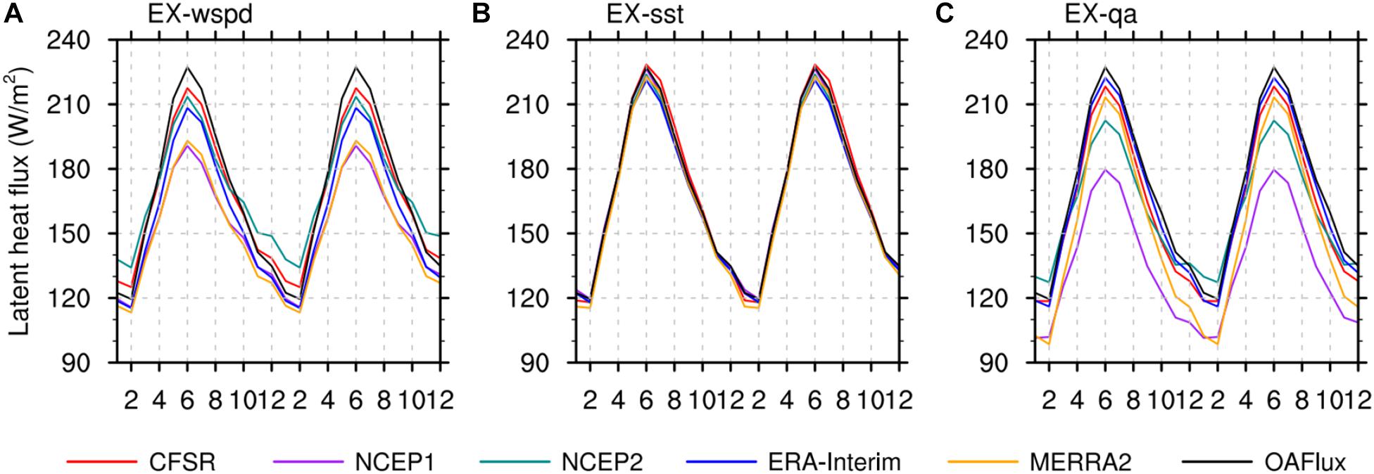
Figure 5. Climatological seasonal cycle of latent heat flux (into the atmosphere) over the region (110°E-116°E, 22°S-32°S) from (A) EX-wspd, (B) EX-sst, (C) EX-qa.

Air-Sea Fluxes Associated With Ningaloo Niño

In the previous subsection, large uncertainties of air-sea fluxes are identified in the climatological seasonal cycle. In this subsection, surface heat fluxes associated with the Ningaloo Niño, which is the major interannual variability in this region, are investigated and their uncertainties are determined using the same datasets.

Ningaloo Niño events are identified based on the Ningaloo Niño Index (NNI) defined as the average of SST anomalies over the region 110°E-116°E, 22°S-32°S (Marshall et al., 2015). Years when the DJF averaged NNI is above one standard deviation are defined as the Ningaloo Niño years. For the entire period of the analysis, six events are identified: 1988/89, 1996/97, 1999/2000, 2010/11, 2011/12, and 2012/13 (Figure 6). The composite time series of surface heat flux anomalies, which cover the period of onset, development, and recovery of the events, are constructed by averaging all six events. Month 0 in the composite is defined as the month of the maximum positive SST anomaly in the region used for the NNI calculation.

FIGURE 6

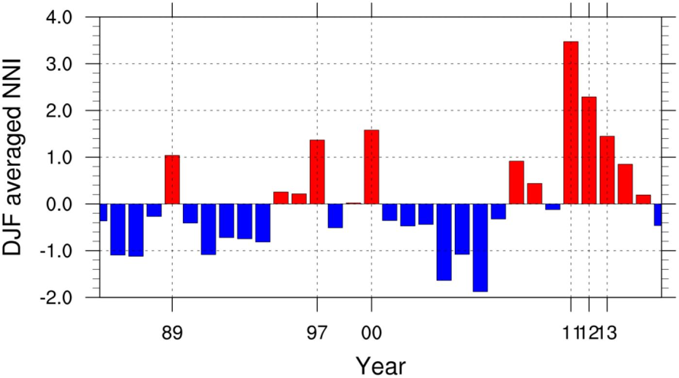
Figure 6. DJF averaged Normalized Ningaloo Niño Index calculated from the NOAA 1/4° daily Optimum Interpolation Sea Surface Temperature. The year shown in the horizontal axis corresponds to the year of January and February.

Despite the large uncertainties in climatology, anomaly fields show much smaller differences between the datasets. However, these uncertainties are still significant because they are in the same order of the amplitude of the anomaly particularly during the warming period. In addition, the sign of the latent heat flux anomalies varies between the datasets during the developing phase of Ningaloo Niño, suggesting the opposite role of latent heat flux. Large variations associated with the Ningaloo Niño are detected in all datasets (Figure 7). For instance, during the developing phase, a significant increase of net surface heat flux is found from month -3 to -2 and month -1 to 0. Then the anomalous surface heat flux decreases sharply from month 0 to month +1, resulting in substantial cooling during the recovery phase (Figure 7A). The sharp decrease (cooling) in the recovery phase is seen clearly in all datasets and it is dominated by the latent heat flux anomaly fluctuation (Figures 7B–E). Similar variations are found for the composite using turbulent heat fluxes from OAFlux and shortwave and longwave radiation from CERES (not shown), but only the last three events are used for this composite because of the shorter period the CERES data cover.

FIGURE 7

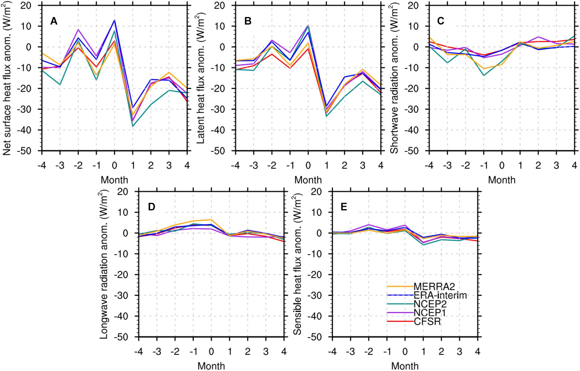
Figure 7. Composites of the monthly mean net surface heat flux (A), latent heat flux (B), shortwave radiation (C), longwave radiation (D) and sensible heat flux (E) anomalies over the region (110°E-116°E, 22°S-32°S) for Ningaloo Niño years. The sign of the longwave radiation, latent and sensible heat flux has been adjusted so that positive values indicate the warming of the ocean. Month 0 is the month of the maximum positive SST anomaly.

To further examine how the fluctuation of the latent heat flux associated with the Ningaloo Niño event occurs, spatial patterns of surface wind anomalies are compared with those of climatological surface winds (Figure 8). During December-April, climatological southeasterly winds prevail around the west coast of Australia. When the Ningaloo Niño is fully developed at month 0, the northerly wind anomalies reach the peak, which largely decrease the climatological southeasterly and thus reduce the wind speed. Such reduction of wind speed is also found in month -2 although it is much weaker. The latent heat flux anomalies from some of the datasets are positive during the development and peak phases due to the weakening of surface winds described above, which are consistent with the windspeed-evaporation-SST (WES) feedback mechanism suggested in previous studies (e.g., Nicholls, 1979; Marshall et al., 2015). However, the positive latent heat flux anomalies are not found in some of the datasets during this period.

FIGURE 8

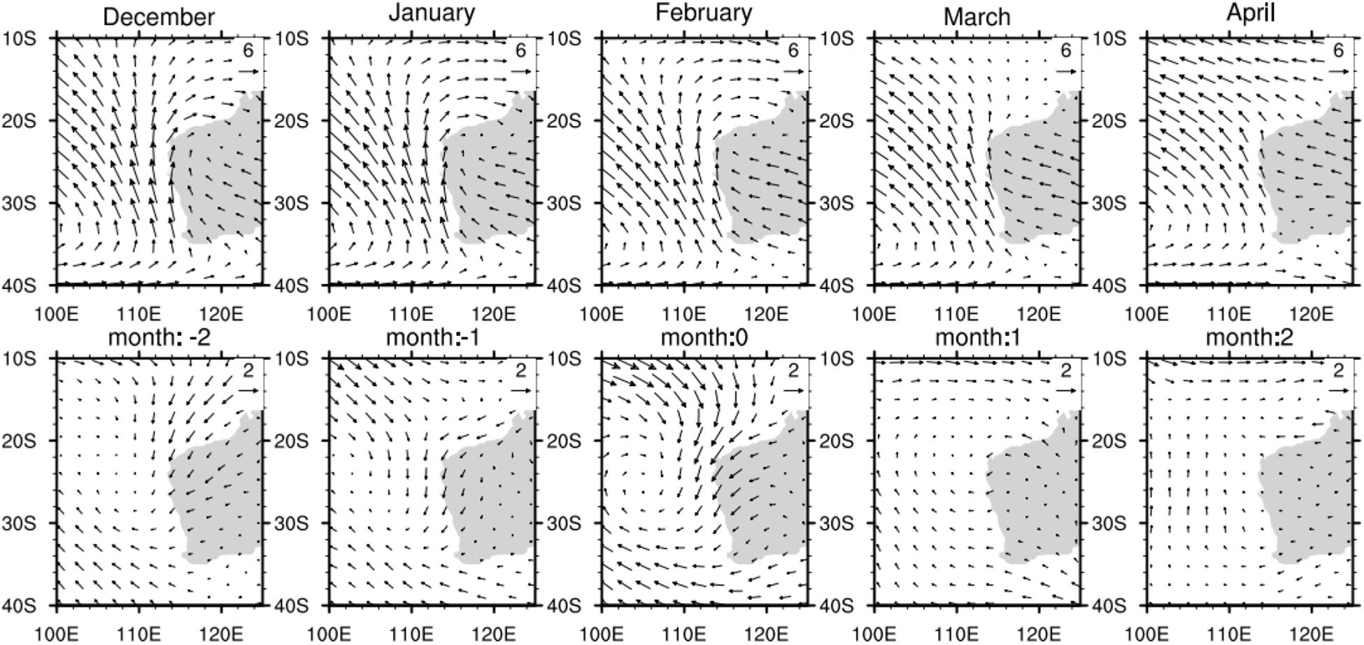
Figure 8. Upper panels: Climatological monthly surface winds. Lower panels: Composite of surface wind anomalies (m/s) for Ningaloo Niño years. Surface winds from ERA-Interim are used for the analysis.

During month +1 soon after the peak, the wind anomaly rapidly changes to weak southerly, resulting in an increase of wind speed by 1 m/s. Since SSTs recover much more slowly and thus they are still anomalously high in month +1 (Figure 9E), the evaporative cooling (negative latent heat flux anomaly) is rapidly enhanced, which contributes to the SST cooling. By month +2, evaporative cooling is reduced because of the decrease of SST although wind speed similar to month +1 is maintained. The variation of latent heat flux anomaly including the rapid increase of negative anomalies in month +1 are found in all datasets. The cooling anomalies in longwave radiation and sensible heat flux, which are associated with high SSTs, are found (Figures 7D,E), but their contributions to SST recovery are much smaller than those of latent heat flux.

FIGURE 9

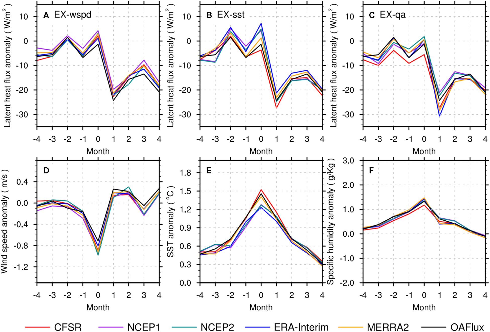
Figure 9. The top row: The composites of monthly heat flux anomalies over the region (110°E-116°E, 22°S-32°S) from (A) EX-wspd, (B) EX-sst and (C) EX-qa. Positive values indicate the warming of the ocean. The bottom row: The wind speed anomalies (D), SST anomalies (E), and specific humidity anomalies (F) from the reanalysis datasets.

In contrast to the recovery phase, the variation of latent heat flux and its contribution to SST growth during the developing phase show disagreement between the datasets. NCEP1 shows warming anomalies during month -2 to 0, while others reveal cooling anomalies (CFSR, MERRA2) or alternate between cooling and warming (NCEP2, ERA-Interim). It is not clear whether the latent heat flux anomaly significantly contributes to the SST warming during the Ningaloo Niño onset. These results are consistent with those of previous studies, which used different surface heat flux products and concluded different roles of surface heat fluxes during the onset and development phases (e.g., Feng et al., 2013; Marshall et al., 2015; Kataoka et al., 2017).

The major sources of the uncertainty during the onset period are further investigated based on the additional analysis using EX-wspd, EX-sst and EX-qa described in Section “Climatology.” Composites of latent heat flux anomalies from EX-wspd, EX-sst and EX-qa are displayed in Figure 9. The mean of the difference between the maximum and minimum latent heat flux anomaly during the entire period of composite is 4.1, 4.7 and 5.0 W m^-2 for EX-wspd, EX-sst and EX-qa, respectively. This suggests that air specific humidity errors could cause larger uncertainties of latent heat flux anomalies, which is similar to the results from the analysis of climatological latent heat flux. However, the largest differences between the datasets during the peak phase are found in EX-sst (Figure 9B), which is 10.9 W m^-2, and the sign of latent heat flux anomaly also shows a disagreement between the datasets. While a significant difference (7.4 W m^-2) is also found in EX-qa in month 0, the sign of the latent heat flux anomaly is the same in most datasets. This result indicates that the uncertainties in SST significantly contribute to the errors in latent heat flux during this period. Since the SST is highest at the peak month, the latent heat flux is most sensitive to changes in SSTs during this period. In other words, even small errors in SST could impact the latent heat flux significantly during the onset and peak periods.

The SST difference between the datasets is largest in the peak period (month 0) (Figure 9E). While SSTs used in the flux products are based on similar satellite observations, their spatial resolutions could influence the accuracy since SST in this region is largely affected by Leeuwin Current variability (Huang and Feng, 2015). Such SST differences caused by the resolution are demonstrated for the 2010–2011 Ningaloo Niño case. The monthly latent heat flux and SST anomaly during the event are shown in Figure 10. To exclude the latent heat flux uncertainties caused by algorithm, wind speed, and humidity, we use fluxes from EX-sst instead of the original reanalysis. In addition to SST products used in the original EX-sst, high resolution OISST and MUR are also included in this case study.

FIGURE 10

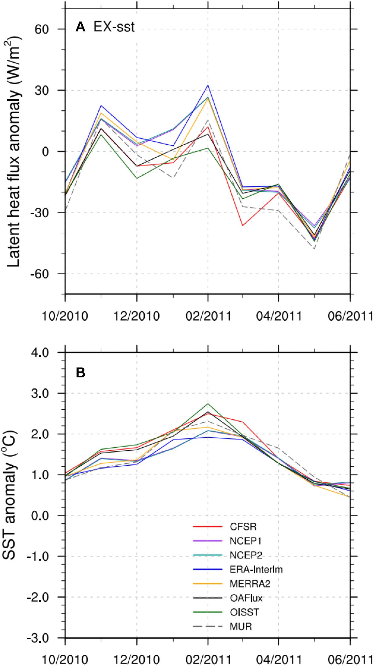
Figure 10. (A) Monthly mean latent heat flux anomalies over the region (110°E-116°E, 22°S-32°S) for the 2010/2011 Ningaloo Niño event from EX-sst. Positive values indicate the warming of the ocean. (B) The corresponding SST anomalies from reanalysis products and satellite observations.

The peak of this Ningaloo Niño occurred in February 2011. From November 2010 to February 2011, warm SST anomalies were built up near the west coast of Australia (Figure 10B). During this time, significant positive latent heat flux anomalies (10–30 W m^-2, positive value denote heat going into the ocean) are evident in NCEP1, NCEP2, ERA-Interim and MERRA2, suggesting that air-sea fluxes may contribute to the SST warming. In contrast, CFSR, OAFlux, MUR and OISST show very small positive anomalies into the ocean, or even negative anomalies in December 2010 and January 2011 (Figures 10A, 12). These differences are caused by warmer area average SSTs for the relatively high-resolution SST products (MUR, OISST) (Figure 10B).

Figure 11 shows SST maps from different datasets during the peak period of the 2010–2011 Ningaloo Niño event. The southward extension of warm waters carried by the Leeuwin Current is evident clearly in the high-resolution data (MUR and OISST), while it is not well represented in the low-resolution data. Accordingly, higher area average SSTs and thus higher evaporative cooling are found in the case of high-resolution SSTs (Figure 12). The results demonstrate that it is crucial to resolve SST changes caused by Leeuwin Current variability adequately for the latent heat flux estimates especially during the peak period of Ningaloo Niño.

FIGURE 11

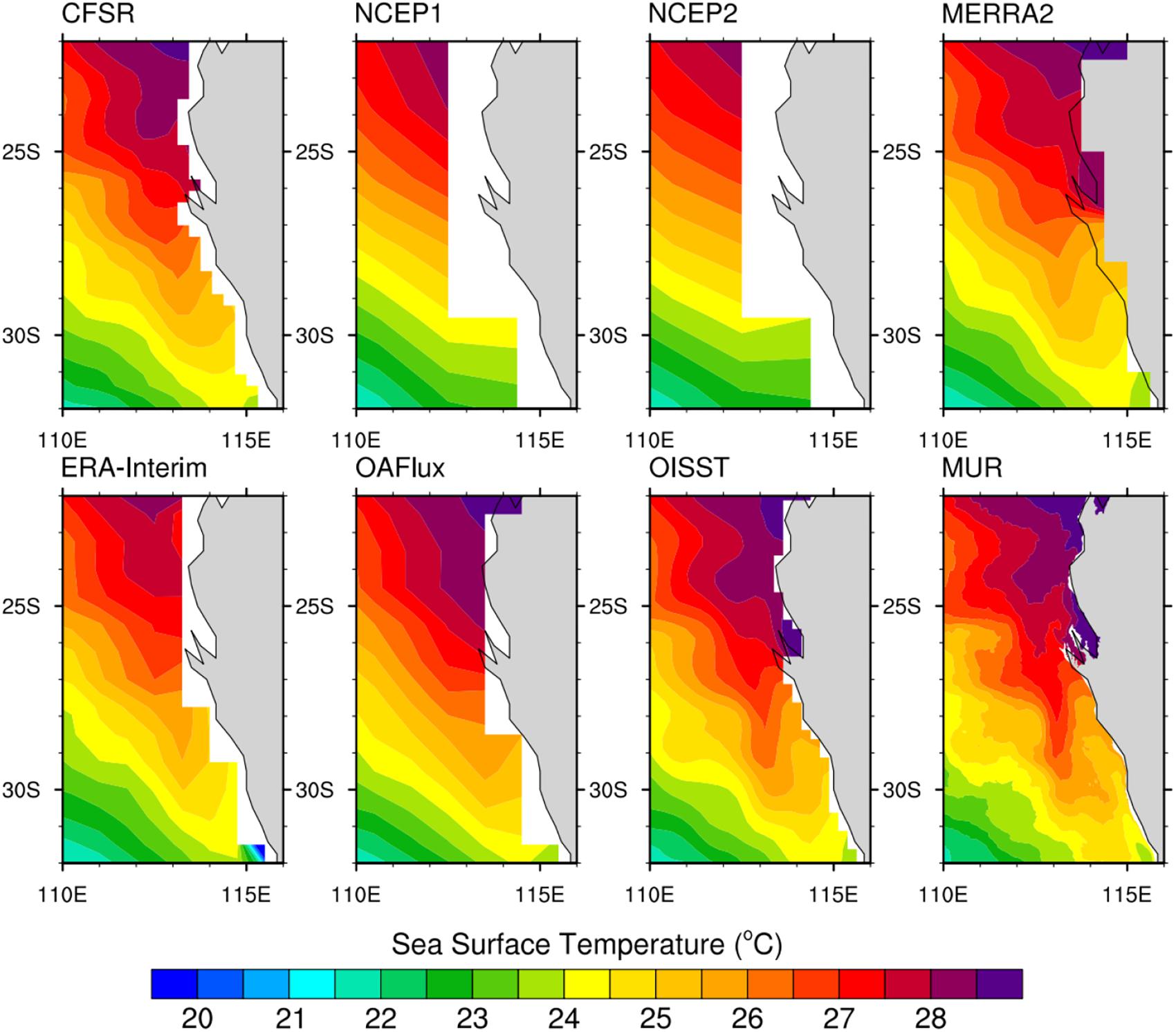
Figure 11. Mean SST of January and February 2011 over the west coast of Australia from different SST datasets.

FIGURE 12

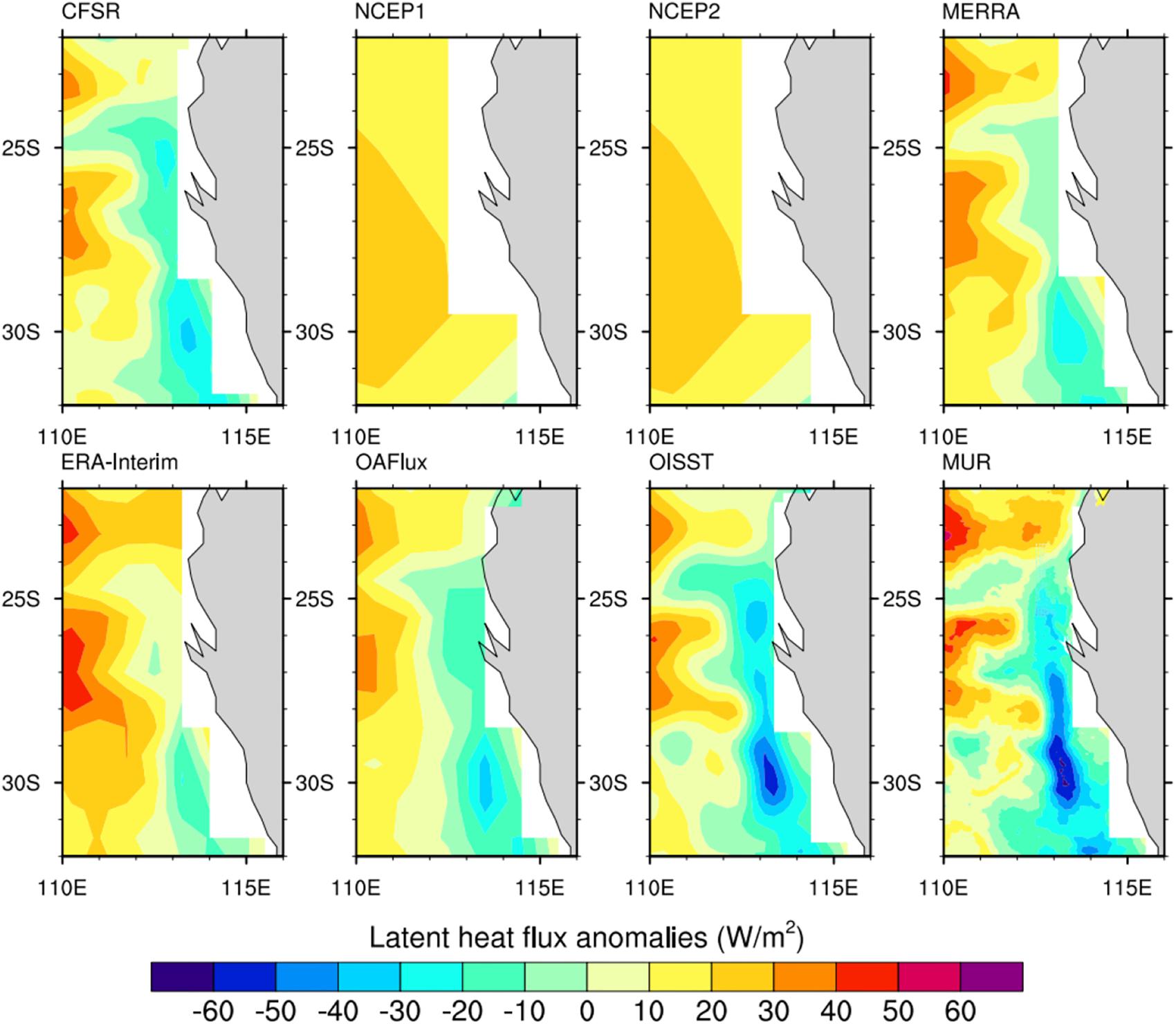
Figure 12. Mean latent heat flux anomalies of January-February 2011 over the west coast of Australia from EX-sst. Positive values indicate the warming of the ocean.

Discussion

The results in the previous section demonstrate that large negative surface heat flux anomalies are found during the decay periods of the Ningaloo Niño in all datasets, and that the latent heat flux anomaly is the dominant component. Such large latent heat fluxes (evaporation) could significantly impact the atmospheric conditions and circulation.

In addition to the air-sea flux anomalies, MLD changes associated with the Ningaloo Niño could influence the SST evolution (Kataoka et al., 2017). Kataoka et al. (2017) suggested that the cooling due to latent heat flux anomalies during the decay period could be largely reduced by MLD variability, and the sensible heat flux significantly contributes to the SST cooling for some events.

To further investigate the relative importance of latent and sensible heat fluxes for the SST variations during the decay phase, these flux terms in the following mixed layer heat budget equation are calculated (Equation 7 in Kataoka et al., 2017):

${\mathrm{\left(}\frac{\mathit{Q}}{{\mathrm{\rho }\mathit{c}}_{\mathit{p}}\mathit{h}}\mathrm{\right)}}^{\mathrm{\prime }}\mathrm{=}\frac{{\mathit{Q}}^{\mathrm{\prime }}}{{\mathrm{\rho }\mathit{c}}_{\mathit{p}}\overline{\mathit{h}}}\mathrm{-}\frac{\overline{\mathit{Q}}}{{\mathrm{\rho }\mathit{c}}_{\mathit{p}}\overline{\mathit{h}}}\frac{{\mathit{h}}^{\mathrm{\prime }}}{\mathit{h}}\mathrm{+}\mathit{Re}\mathit{s}\mathrm{}\mathrm{\left(}\mathrm{1}\mathrm{\right)}$

where Q is the surface heat flux, ρ is seawater density, c_p is the specific heat of seawater, h is the MLD. An overbar represents monthly climatology and a prime represents anomaly. The first term on the RHS represents the contribution of the surface heat flux anomaly, and the second term represents the contribution of MLD variability through the change of the mixed layer heat capacity. The MLD is derived from the HYCOM reanalysis which is defined as the smaller depth at which the temperature is decreased by 0.2°C or the salinity is increased by 0.03 psu from the surface values. The seasonal variation of MLD from the HYCOM reanalysis agrees well with observations (e.g., CARS, Supplementary Figure 1). The composite latent and sensible heat flux anomalies, which include the effect of MLD changes, are shown in Figure 13, and the composites of the first and second term on the RHS of Eq. (1) are shown in Figure 14. Significant contributions of MLD changes are evident (Figures 13, 14). For example, the weak cooling (negative anomaly) is found during the onset and peak phase in the latent heat flux term (Figure 13) in all datasets whereas the weak warming is found in some datasets when the effect of MLD change is not included (Figure 7). The contribution of the MLD change (second term) is relatively large during the onset and peak phase as the first term is small. Yet the latent heat flux term is still dominant and contributes to the cooling during the decay period much more than the sensible heat flux term. The variation of latent heat flux in Figure 13 is similar to that of non-locally amplified Ningaloo Niño in Kataoka et al. (2017). It should be noted that there are no significant differences between locally and non-locally amplified modes in the analysis of this study.

FIGURE 13

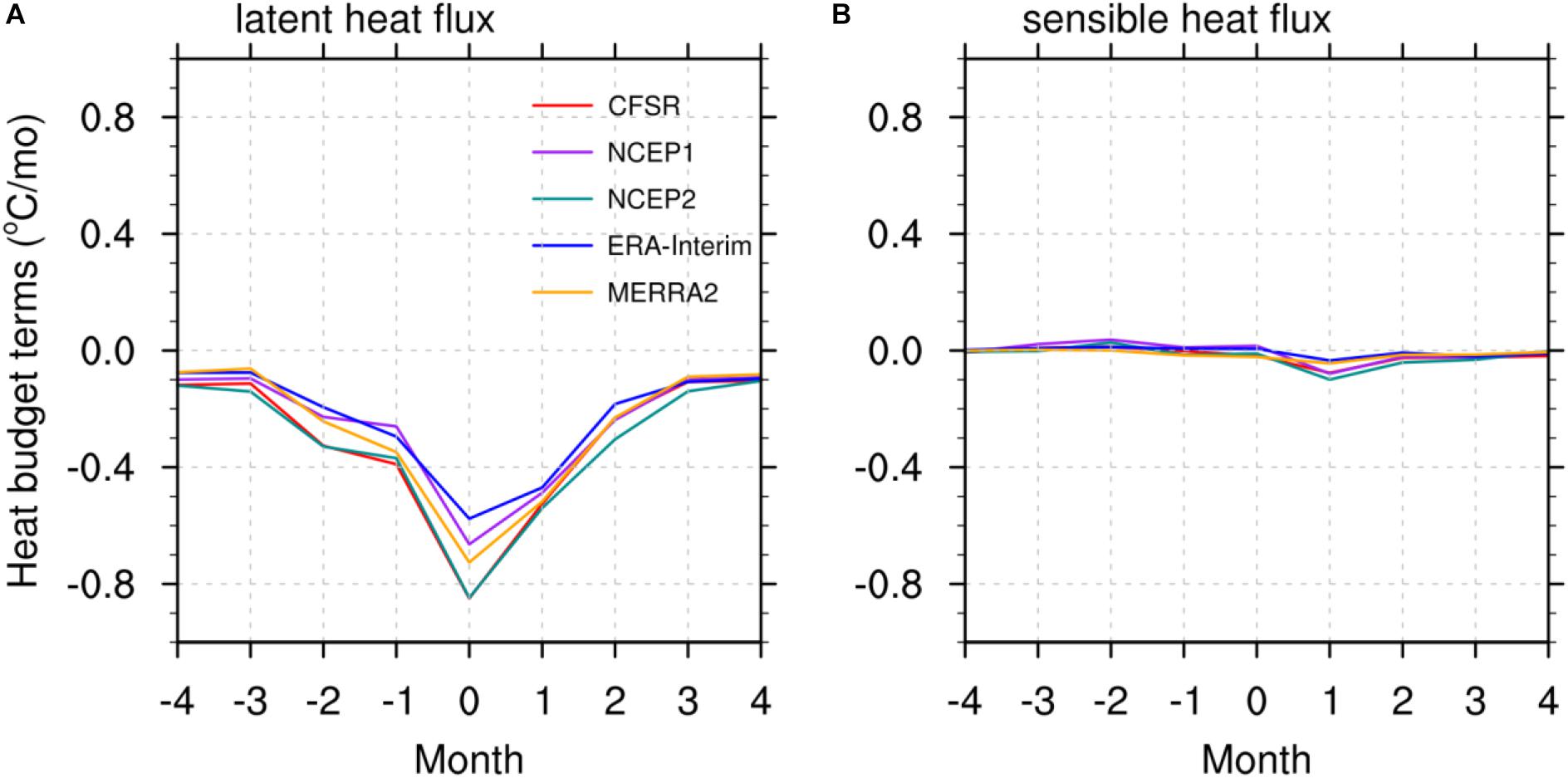
Figure 13. Composites of monthly mean heat flux anomaly term in the mixed layer heat budget equation over the region (110°E-116°E, 22°S-32°S): (A) latent heat flux term, (B) sensible heat flux term.

FIGURE 14

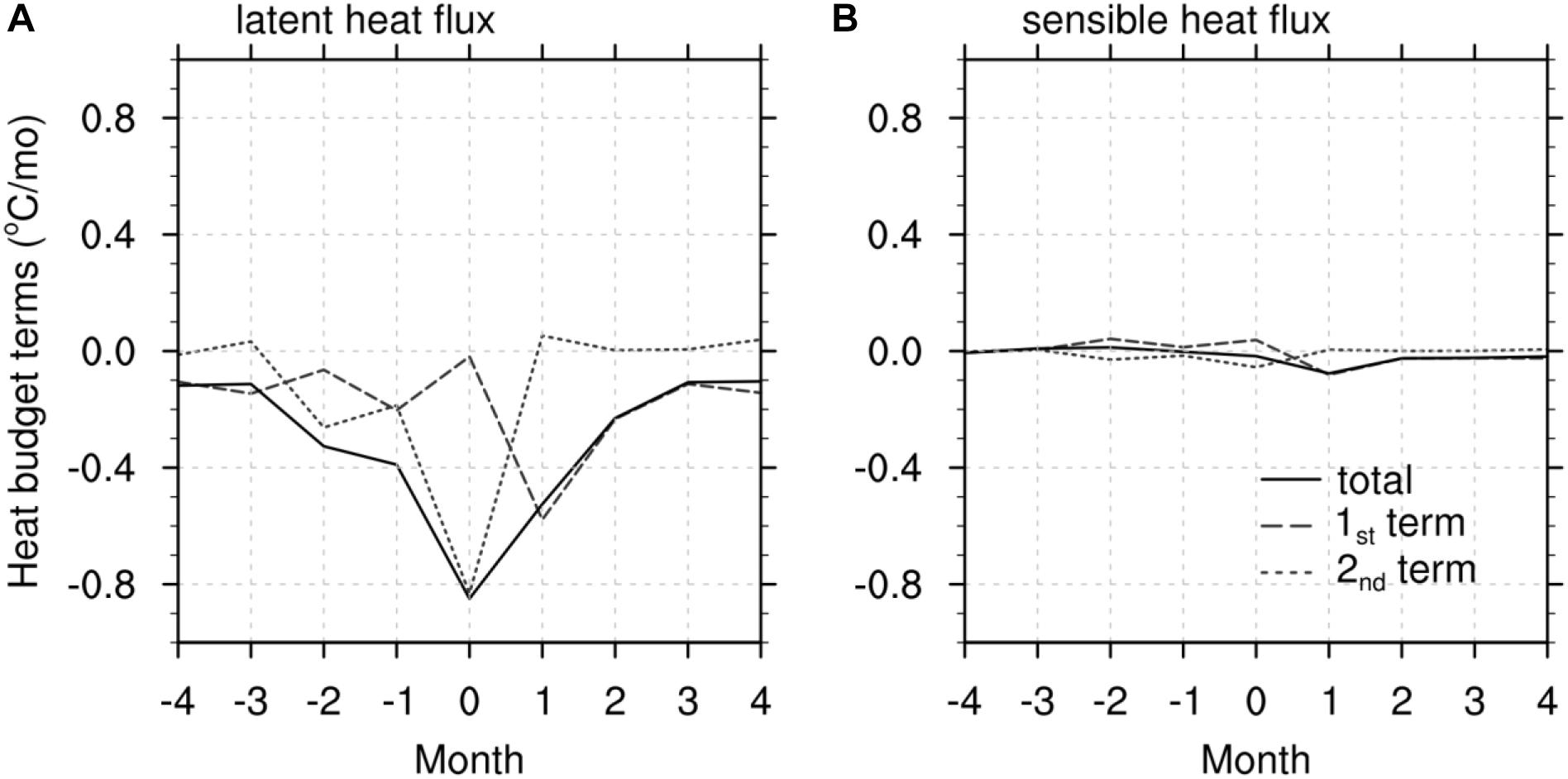
Figure 14. Composite monthly mean heat flux anomaly terms calculated from the mixed layer heat budget equation for the region (110°E-116°E, 22°S-32°S): (A) latent heat flux, (B) sensible heat flux. First and second terms on the RHS of Eq. (1) are compared. Only the results from CFSR are shown. The first term represents a temperature tendency produced by the flux anomaly with the climatological MLD, and the second term represents a temperature tendency produced by climatological fluxes and the MLD anomaly.

Although the reason for the differences between the results of this study and Kataoka et al. (2017) is unknown, it is likely that different sources of the data including air-sea fluxes and MLD are primarily responsible for the differences. In particular, the interannual variation of MLD could be largely model dependent. Thus, further studies which focus on the interannual variability of upper ocean structures including the MLD are necessary.

While earlier studies suggest that a reduction of latent heat flux partially contributes to SST anomalies at the peak of Ningaloo Niño, an opposite conclusion could be obtained when taking account of MLD variation. Figure 13 shows that the latent heat flux damps SST anomalies in all stages of Ningaloo Niño and the cooling reach the maximum during the peak. At the peak phase, large differences in latent heat flux anomaly between the datasets and thus large uncertainties are found. Again, these uncertainties are likely to be related to the resolution of SST.

In addition to the influence of air-sea fluxes on the upper ocean temperature, these heat and moisture fluxes directly affect the atmosphere. In particular, the latent heat fluxes (evaporation) could largely contribute to moisture budget changes in the atmosphere during the period of Ningaloo Niño and thus air-sea interaction. A recent modeling study demonstrates that the Ningaloo Niño could develop without ENSO, and the intrinsic air-sea interaction alone may induce atmospheric cyclonic circulation anomalies and a stronger Leeuwin Current (Kataoka et al., 2018). As the present study suggests the importance of the resolution of SST for the latent heat flux estimates off the west coast of Australia, coupled model simulations using the high-resolution ocean component would be useful to investigate the feedbacks between the atmosphere and ocean that control the development of Ningaloo Niño.

Summary

This study investigates the air-sea flux variability off the west coast of Australia using multiple datasets and satellite observations. We found large uncertainties in climatological net surface heat fluxes. The uncertainties result primarily from latent heat flux and shortwave radiation. The possible causes of the uncertainty for latent heat flux are investigated with additional calculations which isolate the effects of wind speed, SST, humidity, and bulk flux algorithm. The results of these calculations suggest that the use of different bulk flux algorithms largely contributes to the uncertainties. The bulk atmospheric variables also significantly contribute to the uncertainties.

The role of air-sea fluxes in the development and decay of Ningaloo Niño is investigated based on the composite analyses over the life cycle of Ningaloo Niño. Large differences in air-sea flux anomaly fields associated with the Ningaloo Niño between the datasets are evident although they are smaller than the climatology. Large negative air-sea heat flux anomalies (cooling the ocean) in the recovery phase are found in all datasets, and the anomalous latent heat flux is the dominant component. This suggests that the latent heat flux plays an important role in damping the positive SST anomalies during the recovery stage. The composite evolution of surface winds suggests that WES feedback is responsible for the variations of latent heat flux. Since SSTs recover much more slowly than surface winds after the peak of SST warming, large evaporative cooling is favored under the condition of strong winds and warm SST especially during the early stage of the recovery phase. Then the evaporative cooling is reduced as the SST gradually recovers.

During the developing phase, however, the contributions of air-sea heat flux have large uncertainties. Sensitivity calculations show that the differences in SST anomaly between the datasets largely contribute to the uncertainties. Large uncertainties around the period of SST peak are partly due to the warmer SST than other periods, since the small errors in SST could generate large latent heat flux changes. Also, SST anomalies are directly related to the strengthening of the Leeuwin Current, and thus the resolution of SST datasets significantly affects the SST anomalies. A case study of the 2010–2011 Ningaloo Niño event demonstrates a close relationship between the SST anomaly and the resolution of the datasets. Southward extension of warm waters transported by the Leeuwin Current can be adequately resolved only by high-resolution SST datasets. As a result, a relatively cold SST and thus smaller evaporative cooling are estimated using the low-resolution SST datasets.

Author Contributions

Both authors conceived and designed most of the analyses. XF analyzed the data and wrote the manuscript. TS contributed to the discussion of the results and assisted in writing.

Funding

This work was funded by NSF grant OCE-1658218 and NASA grant NNX17AH25G. TS is also supported by NOAA grants NA15OAR431074 and NA17OAR4310256.

Conflict of Interest Statement

The authors declare that the research was conducted in the absence of any commercial or financial relationships that could be construed as a potential conflict of interest.

Acknowledgments

Computing resources were provided by the Climate Simulation Laboratory at NCAR’s Computational and Information Systems Laboratory, sponsored by NSF, and the HPC systems at the Texas A&M University, College Station and Corpus Christi. The NCEP Reanalysis 1 and 2 data are provided by the NOAA/OAR/ESRL PSD, Boulder, CO, United States, from their Web site at https://www.esrl.noaa.gov/psd/. The ERA-Interim, MERRA2 and CFSR reanalysis data are available at ECMWF website https://www.ecmwf.int/en/forecasts/datasets/archive-datasets/reanalysis-datasets/era-interim, the Goddard Earth Sciences (GES) Data and Information Services Center (DISC) (http://disc.sci.gsfc.nasa.gov/mdisc/), and Research Data Archive at the National Center for Atmospheric Research, Computational and Information Systems Laboratory (https://rda.ucar.edu/pub/cfsr.html). OAFlux are provided by the WHOI OAFlux project (http://oaflux.whoi.edu) funded by the NOAA Climate Observations and Monitoring (COM) program. CERES, OISST and MUR SST are obtained from CERES website https://ceres.larc.nasa.gov/order_data.php, NOAA’s NCEI websites https://www.ncdc.noaa.gov/oisst, and https://mur.jpl.nasa.gov, respectively. The RAMA buoy data are obtained at https://www.pmel.noaa.gov/tao/drupal/disdel/.

Supplementary Material

The Supplementary Material for this article can be found online at: https://www.frontiersin.org/articles/10.3389/fmars.2019.00266/full#supplementary-material

References

Banzon, V., Smith, T. M., Chin, T. M., Liu, C., and Hankins, W. (2016). A long-term record of blended satellite and in situ sea-surface temperature for climate monitoring, modeling and environmental studies. Earth Syst. Sci. Data 8, 165–176. doi: 10.5194/essd-8-165-2016

CrossRef Full Text | Google Scholar

Benthuysen, J., Feng, M., and Zhong, L. (2014). Spatial patterns of warming off Western Australia during the 2011 Ningaloo Niño: quantifying impacts of remote and local forcing. Cont. Shelf Res. 91, 232–246. doi: 10.1016/j.csr.2014.09.014

CrossRef Full Text | Google Scholar

Brunke, M. A., Zeng, X., and Anderson, S. (2002). Uncertainties in sea surface turbulent flux algorithms and data sets. J. Geophys. Res. 107, 3141. doi: 10.1029/2001JC000992

CrossRef Full Text | Google Scholar

Caputi, N., Gary, J., and Pearce, A. (2014). The Marine Heat Wave Off Western Australia During the Summer of 2010/11 – 2 Years on. Western Australia, WA: Department of Fisheries. Fisheries Research Report No. 250.

Google Scholar

Chin, T. M., Vazquez-Cuervo, J., and Armstrong, E. M. (2017). A multi-scale high-resolution analysis of global sea surface temperature. Remote Sens. Environ. 200, 154–169. doi: 10.1016/j.rse.2017.07.029

PubMed Abstract | CrossRef Full Text | Google Scholar

Dee, D. P., Uppala, S. M., Simmons, A. J., Berrisford, P., Poli, P., Kobayashi, S., et al. (2011). The ERA-Interim reanalysis: configuration and performance of the data assimilation system. Q. J. R. Meteorol. Soc. 137, 553–597. doi: 10.1002/qj.828

CrossRef Full Text | Google Scholar

Fairall, C. W., Bradley, E. F., Hare, J. E., Grachev, A. A., and Edson, J. B. (2003). Bulk parameterization of air–sea fluxes: updates and verification for the COARE algorithm. J. Clim. 16, 571–591.

Google Scholar

Feng, M., Biastoch, A., Boning, C., Caputi, N., and Meyers, G. (2008). Seasonal and interannual variations of upper ocean heat balance off the west coast of Australia. J. Geophys. Res. 113, C12025. doi: 10.1029/2008JC004908

CrossRef Full Text | Google Scholar

Feng, M., McPhaden, M. J., Xie, S.-P., and Hafner, J. (2013). La Niña forces unprecedented Leeuwin Current warming in 2011. Sci. Rep. 3, 1–9. doi: 10.1038/srep01277

PubMed Abstract | CrossRef Full Text | Google Scholar

Feng, M., Meyers, G., Pearce, A., and Wijffels, S. (2003). Annual and interannual variations of the Leeuwin Current at 32°S. J. Geophys. Res. 108, 3355. doi: 10.1029/2002JC001763

CrossRef Full Text | Google Scholar

Gelaro, R., McCarty, W., Suárez, M. J., Todling, R., Molod, A., Takacs, L., et al. (2017). The modern-era retrospective analysis for research and applications. version 2 (MERRA-2). J. Clim. 30, 5419–5454. doi: 10.1175/JCLI-D-16-0758.1

CrossRef Full Text | Google Scholar

Huang, Z., and Feng, M. (2015). Remotely sensed spatial and temporal variability of the leeuwin current using MODIS data. Remote Sens. Environ. 166, 214–232. doi: 10.1016/j.rse.2015.05.028

CrossRef Full Text | Google Scholar

Kalnay, E., Kanamitsu, M., Kistler, R., Collins, W., Deaven, D., Gandin, L., et al. (1996). The NCEP/NCAR 40-Year Reanalysis Project. Bull. Am. Meteorol. Soc. 77, 437–472.

Google Scholar

Kanamitsu, M., Ebisuzaki, W., Woollen, J., Yang, S.-K., Hnilo, J. J., Fiorino, M., et al. (2002). NCEP–DOE AMIP-II reanalysis (R-2). Bull. Am. Meteorol. Soc. 83, 1631–1644.

Google Scholar

Kataoka, T., Masson, S., Izumo, T., Tozuka, T., and Yamagata, T. (2018). Can Ningaloo Niño/Niña develop without El Niño–Southern oscillation? Geophys. Res. Lett. 45, 7040–7048. doi: 10.1029/2018GL078188

CrossRef Full Text | Google Scholar

Kataoka, T., Tozuka, T., Behera, S., and Yamagata, T. (2014). On the ningaloo niño/niña. Clim. Dyn. 43, 1463–1482. doi: 10.1007/s00382-013-1961-z

CrossRef Full Text | Google Scholar

Kataoka, T., Tozuka, T., and Yamagata, T. (2017). Generation and decay mechanisms of ningaloo niño/niña. J. Geophys. Res. Ocean. 122, 8913–8932. doi: 10.1002/2017JC012966

CrossRef Full Text

Kato, S., Rose, F. G., Rutan, D. A., Thorsen, T. J., Loeb, N. G., Doelling, D. R., et al. (2018). Surface irradiances of edition 4.0 clouds and the earth’s radiant energy system (CERES) energy balanced and filled (EBAF) data product. J. Clim. 31, 4501–4527. doi: 10.1175/JCLI-D-17-0523.1

CrossRef Full Text | Google Scholar

Kubota, M., Iwabe, N., Cronin, M. F., and Tomita, H. (2008). Surface heat fluxes from the NCEP/NCAR and NCEP/DOE reanalyses at the Kuroshio Extension Observatory buoy site. J. Geophys. Res. Ocean. 113, 1–14. doi: 10.1029/2007JC004338

CrossRef Full Text | Google Scholar

Marshall, A. G., Hendon, H. H., Feng, M., and Schiller, A. (2015). Initiation and amplification of the Ningaloo Niño. Clim. Dyn. 45, 2367–2385. doi: 10.1007/s00382-015-2477-2475

CrossRef Full Text | Google Scholar

McPhaden, M. J., Meyers, G., Ando, K., Masumoto, Y., Murty, V. S. N., Ravichandran, M., et al. (2009). RAMA: the research moored array for African-Asian-Australian monsoon analysis and prediction. Bull. Am. Meteorol. Soc. 90, 459–480. doi: 10.1175/2008BAMS2608.1

CrossRef Full Text | Google Scholar

Metzger, E. J., Smedstad, O. M., Thoppil, P., Hurlburt, H., Cummings, J., Walcraft, A., et al. (2014). US navy operational global ocean and arctic ice prediction systems. Oceanography 27, 32–43. doi: 10.5670/oceanog.2014.66

CrossRef Full Text | Google Scholar

Nicholls, N. (1979). A simple air-sea interaction model. Q. J. R. Meteorol. Soc. 105, 93–105. doi: 10.1002/qj.49710544307

PubMed Abstract | CrossRef Full Text | Google Scholar

Pearce, A. F., and Feng, M. (2013). The rise and fall of the “marine heat wave” off Western Australia during the summer of 2010/2011. J. Mar. Syst. 111, 139–156. doi: 10.1016/j.jmarsys.2012.10.009

CrossRef Full Text | Google Scholar

Reynolds, R. W., Smith, T. M., Liu, C., Chelton, D. B., Casey, K. S., and Schlax, M. G. (2007). Daily High-Resolution-Blended Analyses for Sea Surface Temperature. J. Clim. 20, 5473–5496. doi: 10.1175/2007JCLI1824.1

CrossRef Full Text | Google Scholar

Saha, S., Moorthi, S., Pan, H.-L., Wu, X., Wang, J., Nadiga, S., et al. (2010). The NCEP Climate Forecast System Reanalysis. Bull. Am. Meteorol. Soc. 91, 1015–1058. doi: 10.1175/2010BAMS3001.1

CrossRef Full Text | Google Scholar

Saha, S., Moorthi, S., Wu, X., Wang, J., Nadiga, S., Tripp, P., et al. (2014). The NCEP Climate Forecast System Version 2. J. Clim. 27, 2185–2208. doi: 10.1175/JCLI-D-12-00823.1

CrossRef Full Text | Google Scholar

Tozuka, T., Kataoka, T., and Yamagata, T. (2014). Locally and remotely forced atmospheric circulation anomalies of Ningaloo Niño/Niña. Clim. Dyn. 43, 2197–2205. doi: 10.1007/s00382-013-2044-x

CrossRef Full Text | Google Scholar

Tozuka, T., and Oettli, P. (2018). Asymmetric Cloud-Shortwave Radiation-Sea Surface Temperature Feedback of Ningaloo Niño/Niña. Geophys. Res. Lett. 45, 9870–9879. doi: 10.1029/2018GL079869

CrossRef Full Text | Google Scholar

Valdivieso, M., Haines, K., Balmaseda, M., Chang, Y. S., Drevillon, M., Ferry, N., et al. (2017). An assessment of air–sea heat fluxes from ocean and coupled reanalyses. Clim. Dyn. 49, 983–1008.

Google Scholar

Wernberg, T., Smale, D. A., Tuya, F., Thomsen, M. S., Langlois, T. J., De Bettignies, T., et al. (2013). An extreme climatic event alters marine ecosystem structure in a global biodiversity hotspot. Nat. Clim. Change 3, 78–82. doi: 10.1038/nclimate1627

CrossRef Full Text | Google Scholar

Wu, R., Kirtman, B. P., and Pegion, K. (2006). Local air-sea relationship in observations and model simulations. J. Clim. 19, 4914–4932. doi: 10.1175/JCLI3904.1

CrossRef Full Text | Google Scholar

Xu, J., Lowe, R. J., Ivey, G. N., Jones, N. L., and Zhang, Z. (2018). Contrasting Heat Budget Dynamics During Two La Niña Marine Heat Wave Events Along Northwestern Australia. J. Geophys. Res. Ocean. 123, 1563–1581. doi: 10.1002/2017JC013426

CrossRef Full Text | Google Scholar

Yu, L., Jin, X., and Weller, R. A. (2008). Multidecade Global Flux Datasets from the Objectively Analyzed Air-sea Fluxes (OAFlux) Project: Latent and Sensible Heat Fluxes, Ocean Evaporation, and Related Surface Meteorological Variables. Massachusetts: Woods Hole Oceanographic Institution. OAFlux Project Technical Report. OA-2008-01.

Google Scholar

Zeng, X., Zhao, M., and Dickinson, R. (1998). Intercomparison of bulk aerodynamic for the computation of sea surface fluxes using TOGA COARSE and TAO data. J. Clim. 11, 2628–2644.

Google Scholar

Zhang, D., Cronin, M. F., Wen, C., Xue, Y., Kumar, A., and McClurg, D. (2016). Assessing surface heat fluxes in atmospheric reanalyses with a decade of data from the NOAA kuroshio extension observatory. J. Geophys. Res. Ocean. 121, 6874–6890. doi: 10.1002/2016JC011905

CrossRef Full Text | Google Scholar

Zhang, L., and Han, W. (2018). Impact of Ningaloo Niño on tropical pacific and an interbasin coupling mechanism. Geophys. Res. Lett. 45, 11300–11309. doi: 10.1029/2018GL078579

CrossRef Full Text | Google Scholar

Zhang, L., Han, W., Li, Y., and Shinoda, T. (2018). Mechanisms for generation and development of Ningaloo Niño. J. Clim. 31, 9239–9259. doi: 10.1175/JCLI-D-18-0175.1

CrossRef Full Text | Google Scholar

Appendix

Uncertainty of Latent Heat Flux Caused by Bulk Flux Algorithm and Its Seasonality

The bulk flux algorithm calculates latent heat flux by using the mean value of bulk state variables (Yu et al., 2008):

${\mathit{Q}}_{\mathrm{L}\mathrm{H}}\mathrm{=}\mathrm{\rho }{\mathit{L}\mathit{C}}_{\mathrm{e}}\mathit{U}\mathrm{(}{\mathit{q}}_{\mathrm{s}}\mathrm{-}\mathrm{-}{\mathit{q}}_{\mathrm{a}}\mathrm{)}\mathrm{}\mathrm{\left(}\mathrm{2}\mathrm{\right)}$

where ρ is the density of air, L is the latent heat of vaporization, C_e is the transfer coefficient for moisture, U is surface wind speed relative to surface current, q_s is sea surface saturated specific humidity estimated from SST and q_a is air specific humidity. The direction of the latent heat flux calculated with this equation is from the ocean to the atmosphere for the positive values. While latent heat flux is directly proportional to wind speed and humidity gradient, the transfer coefficient for moisture, which represents the physical processes involved in the heat transfer at the air-sea interface, can change with wind speed and atmosphere stability. The transfer coefficient is calculated differently in different algorithms.

Figure A1 shows the uncertainties of latent heat flux caused by the algorithms used in reanalysis products. While latent heat flux based on the algorithm in NCEP1 and NCEP2 have a larger difference compared to that from COARE3.5, CFSR and ERA-Interim indicate a better agreement with COARE3.5. The uncertainties also depend on the magnitude of latent heat flux and larger latent heat flux usually have larger uncertainties. However, results from NCEP1 and CFSR show the uncertainty is larger in summer than in winter, although latent heat flux is higher in winter. This difference between summer and winter is likely due to the difference in wind speed. Zeng et al. (1998) showed that the neutral exchange coefficient for latent heat flux from different algorithms diverge at higher wind speed. During summer, winds are stronger although the latent heat flux is relatively smaller. The wind effect on the transfer coefficient is likely to account for the larger uncertainty during summer.

FIGURE A1

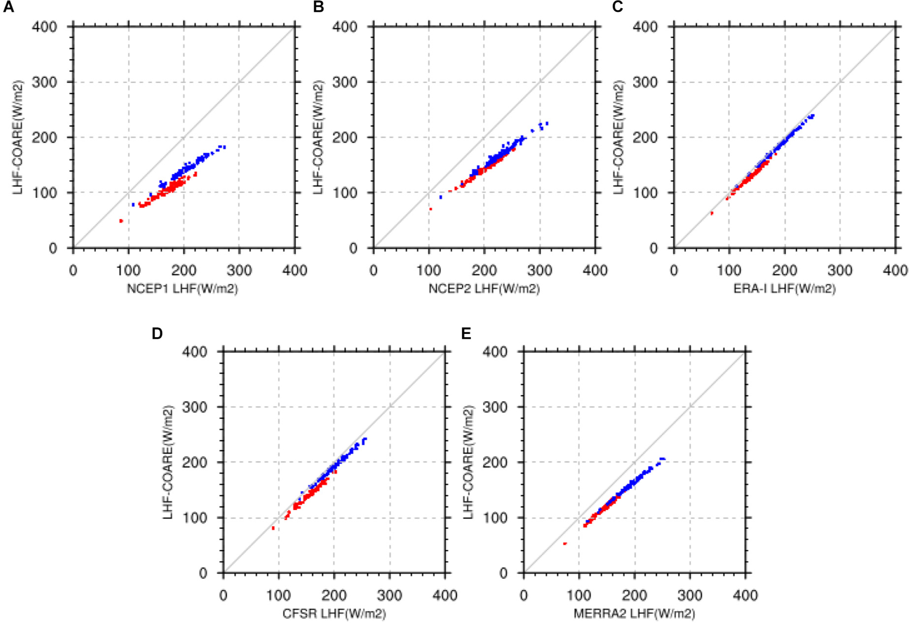
Figure A1. Comparisons of monthly latent heat fluxes (LHF) from EX-alg (vertical axis) with those (horizontal axis) obtained from (A) NCEP1, (B) NCEP2, (C) ERA-Interim, (D) CFSR and (E) MERRA2. JJA (DJF) data points are shown in blue (red).