Monitoring Marine Habitats With Photogrammetry: A Cost-Effective, Accurate, Precise and High-Resolution Reconstruction Method

Introduction

Mapping marine habitats on a large scale has been of primary interest for years as it is essential to estimate, to understand, and to predict biotic assemblages and the distribution of marine biodiversity (Tittensor et al., 2014). To date, knowledge on the patterns and changes of marine biodiversity in Europe and its role in ecosystem functioning has been scattered and imprecise. In the past few years, however, the study of marine biodiversity has risen from relative obscurity to becoming an important issue in European policy and science. The reason is obvious: the seas are not exempt from the impacts of the Anthropocene and the diversity of life in marine ecosystems is rapidly changing (McGill et al., 2015). Nevertheless, most indicators of biodiversity loss relate to the global scale (Pimm et al., 2014), whereas it is locally that biodiversity needs to be monitored in order to capture a potential consistent loss, which is still not properly detected at the global scale (Dornelas et al., 2014). Key data for studying the effects of anthropogenic pressures on the marine environment at different scales, from local to global, is in fact lacking (Halpern et al., 2008). Conversely, two-dimensional maps are insufficient for the understanding of fine scale ecological processes as the structural complexity of benthic habitats has been shown to play a major role in structuring their constitutive ecological assemblages (Friedlander et al., 2003; Kovalenko et al., 2012; Graham and Nash, 2013; Agudo-Adriani et al., 2016; Darling et al., 2017). Besides, monitoring marine habitats requires the accurate measurement of lengths, areas and volumes that are difficult or even impossible to get in situ with traditional methods. A variety of tools and techniques have been used to measure these metrics, from in situ diver measurements (Dustan et al., 2013) to remote sensors such as airborne Lidar (Wedding et al., 2008). These are either punctual with very low spatial resolution (distance between neighbor points/vertices), not accurate enough, or limited to very shallow waters. There is certainly a need for a cost-effective and operational, accurate [closeness of a measurement to the true value (Granshaw, 2016)], precise (low variability, highly reproducible) and high resolution three-dimensional (3D) protocol for capturing the fine-scale architecture of marine habitats.

Modern photogrammetry, also known as structure-from-motion, defines the 3D reconstruction of an object or scene from a high number of photographs taken from different points of view (Figueira et al., 2015). Photogrammetry was first developed for terrestrial applications, and it was later introduced for underwater use by archeologists in the 1970s (Pollio, 1968; Drap, 2012). This technique has seen impressive growth during the last decade and is now extensively used in marine ecology to study interactions between habitat structure and the ecological assemblages (Darling et al., 2017). It has also been used to automatically map the seabed from metrics such as luminance (Mizuno et al., 2017), and simply as a tool for monitoring growth of benthic sessile organisms (Bythell et al., 2001; Chong and Stratford, 2002; Abdo et al., 2006; Holmes, 2008; Gutiérrez-Heredia et al., 2015; Reichert et al., 2016). Based on this technique, recent developments in hardware and image processing have rendered possible the reconstruction of high-resolution 3D models of relatively large areas (1 ha) (Friedman et al., 2012; González-Rivero et al., 2014; Leon et al., 2015). However, the underwater environment is still challenging due to many factors: no GPS information is available to help positioning the photographs, light refraction reduces the field of view and makes necessary the use of a wide angle lens that increases image distortions (Guo et al., 2016; Menna et al., 2017), and large lighting and water clarity variations affect the image quality and consequently the calculation of the position and orientation of the photographs (i.e., bundle adjustment) (Bryson et al., 2017). Despite these environmental constraints, many studies showed relatively accurate 3D models reconstructed with photogrammetry, notably individual scleractinian corals (2–20% accuracy for volume and surface area measurements, depending on colony complexity) (Bythell et al., 2001; Cocito et al., 2003; Courtney et al., 2007; Lavy et al., 2015; Gutierrez-Heredia et al., 2016).

Monitoring benthic biodiversity through 3D reconstruction requires a sub-centimetric to millimetric resolution, with a corresponding accuracy (closeness to true positions/measures) and precision (variability of positions/measures). This is because some habitats are highly complex in structure and have low growth such as coral reefs (Pratchett et al., 2015) or coralligenous reefs (Sartoretto, 1994; Garrabou and Ballesteros, 2000; Ballesteros, 2006). In order to be able to monitor these important habitats for biodiversity, very high-resolution and accurate reconstructions to detect slow growth or small changes in structure over time are needed. Nevertheless, improve resolution and accuracy comes at a cost. In this instance, the finer the resolution for a given surface area, the more time-consuming the modeling process is, and with a very high number of images the reconstruction software can even reach the machine limits (Agisoft, 2018). Ultimately, large photogrammetric models are usually made to the detriment of the final resolution and require expensive, hard to deploy “Underwater autonomous vehicles” (UAV) (Johnson-Roberson et al., 2010). There is consequently a need to strike a balance between a robust and highly accurate protocol, and a methodology that remains relatively low-cost and time-effective, in order to map numerous sites within a large-scale monitoring system. The correlation between local ecological processes, quantified on punctual 3D models, and continuous macro-ecological variables available at broader scale, could help better understand and manage marine biodiversity of entire regions (González-Rivero et al., 2016).

Over the last decade, many research teams have developed their own methodology, some using monoscopic photogrammetry (Burns et al., 2015a, b, 2016; Figueira et al., 2015; Gutiérrez-Heredia et al., 2015), and some using stereo photogrammetry (Abdo et al., 2006; Ferrari et al., 2016; Bryson et al., 2017; Pizarro et al., 2017). Others have worked on the effect of trajectory (Pizarro et al., 2017), camera orientation (Chiabrando et al., 2017; Raczynski, 2017), and camera system (Guo et al., 2016) on the resulting model accuracy. Others focused on the repeatability of measurements such as volume (Lavy et al., 2015) and surface rugosity in different environmental conditions (Bryson et al., 2017). Most of these studies had the same goal underpinning: estimating the accuracy and precision of the models and their derived metrics, and eventually assessing the effect of a given driver. If some of these effects are well documented in traditional photogrammetry, there is still a lack of knowledge on their transposition below the surface. Indeed, underwater photogrammetry remains understudied. Moreover, none of the underwater studies explicitly tested different configuration arrangements on one given study area in order to assess the relative effects of all the parameters on the model, including resolution, accuracy and precision. Knowing the best possible results in underwater conditions remains a research gap. Recently, an effort has been made to assess the influence of photo density (the number of photos per m²) on volume-area (Raoult et al., 2017) and rugosity measurements (Bryson et al., 2017). Although most software manuals recommend a minimum overlap between photos to ensure correct bundle adjustments and accurate models [80% overlap + 60% side-overlap (Agisoft, 2018)], it proved difficult to quantify the influential factors. So far it seems that no study about underwater photogrammetry has considered either the effect of flying elevation, or the total processing time (TPT) of the images as criteria for the definition of an operational and cost-effective monitoring method. These two factors are yet crucial to take into account as they are likely to affect both model resolution and the capacity to monitor numerous sites.

Based on monoscopic multi-image photogrammetry, this study aims to define an operational, cost-effective methodology of producing high-resolution models of surfaces ranging between a few square meters to 500 m², in order to monitor marine biodiversity of temperate and tropical habitats. This study will define a method that is easy to handle, compatible with off-the-shelf commercial softwares, with a sub-centimetric resolution and the lowest processing time possible. Through the setup of two experiments, we tested in natura the influence of the camera system, flying elevation, camera orientation and photo density on the resolution, accuracy and precision of 3D reconstructions. More particularly, this study addresses the following questions:

(1) What is the relative influence of camera system, flying elevation, camera orientation and photo density on:

(a) The accuracy of bundle adjustment?

(b) The number of points in the dense cloud?

(c) The model resolution?

(2) What is the best value for the photo density considering the trade-off between accurate bundle adjustment, high dense cloud size, high resolution and low processing time?

(3) Having considered the best combination of these parameters in relation to the photo density, what is the expected accuracy and precision for:

(a) The XYZ positioning of markers?

(b) The measures of length, area and volume?

(c) The reconstruction of 3D geometries?

Materials and Methods

Two experiments were carried out. The first experiment (hereafter referred to as “experiment 1”) entailed testing all combinations of the parameters and assessing their relative effects on the accuracy of the bundle adjustment and model resolution. The second experiment (hereafter “experiment 2”) entailed measuring the accuracy and precision of the models, reconstructed with the best combination of parameters found in experiment 1. The process flow diagram is illustrated in Figure 1.

FIGURE 1

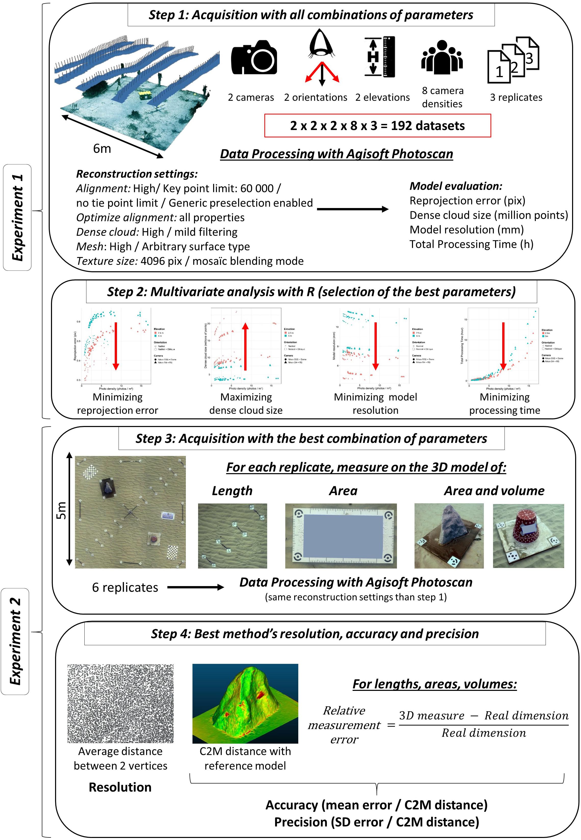
Figure 1. Flow diagram of the methodology. C2M, Cloud-to-mesh.

Experimental Design

Experiment 1: Defining the Best Set of Parameters for Acquisition

The first experiment tested different combinations of parameters, assessing their relative effects on the accuracy of bundle adjustment and model resolution. The experiment took place at 15 m depth in the Mediterranean Sea (Calvi bay, Corsica, France) and corresponded to a 6 × 6 m patch of sand in between dense Posidonia oceanica meadows, with a mixture of existing artificial structures and objects placed across the area. All acquisitions were conducted using two different cameras:

• A Nikon D3S in a waterproof Seacam housing, mounted with a Nikon 20 mm fixed lens and a hemispherical dome port (hereafter referred to as “Nikon D3S + Dome,” see details Table 1).

• A Nikon D4 in a waterproof Seacam housing, mounted with a Nikonos RS 20–35 mm marine lens (hereafter referred to as “Nikon D4 + RS,” see details Table 1).

TABLE 1

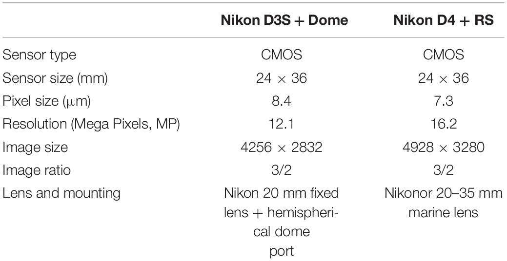
Table 1. Camera systems specifications.

The diver flew at two different elevations over the horizontal area (2.5 and 5 m above the seafloor, following a depth gauge), describing parallel and regularly spaced transects, commonly known as the “mow the lawn” method (Pizarro et al., 2017). He flew at a relatively low speed of 20–25 m/min with a time lapse of 0.5 s between pictures. Each acquisition was done in two steps: (i) a first with nadiral orientation (i.e., vertical downward) and (ii) a second with oblique orientation. Nadiral acquisition involved a single path along each transect, and oblique acquisition involved two paths per transect (one toward right, and the other toward the left). Oblique photos were taken with an angle of approximately 30° from vertical.

All combinations of parameters (camera, elevation and orientation) were performed with three replicates per combination, to distinguish intrinsic and extrinsic variabilities. In total, this represents 24 photo datasets. For each dataset, eight sub-datasets were generated by uniformly sampling one over N images (1 ≤ N ≤ 8) to study the effect of photo density on the accuracy of bundle adjustment and model resolution. We ran all models with 100, 50, 33, 25, 20, 17, 14, and 12.5% of photos, which represents a total of 192 models ranging from 23 to 594 photos (see step 1 in Figure 1). For a given subsampling level (%), datasets constituted of both nadiral and oblique photos, by definition, resulted in higher camera densities than pure nadiral. All models were orientated and sized with a 1 × 1 m cross scale bar located in the center of the study area, and were aligned together with four 10 × 10 cm coded markers placed at the corners. The scale bar length was of the same magnitude as the edge of the scanned area (1 m vs. 6 m) (VDI / VDE, 2002). All models were produced within the same spatial extent (i.e., same bounding box), defined by the positions of the four markers placed at the corners of the study site.

Camera settings were adjusted to achieve a sufficient balance between depth of field, sharpness, and exposure, with the constraint of a high shutter speed to avoid image blurring (20 mm focal length, F10, 1/250 s, ISO 400). Focus was set automatically at the beginning of each acquisition, then turned to manual.

Experiment 2: Measuring the Accuracy and Precision With the Best Set of Parameters

The aim of the second experiment was to evaluate the accuracy and precision of the models by assessing the variability in the positioning of coded markers, and comparing measurements and 3D geometries of true and modeled objects, using the best combination of parameters obtained in experiment 1. The site was located at 15 m depth in the Mediterranean Sea (Roquebrune Bay, next to Cap Martin, France) and corresponded to a 5 × 5 m sandy area, equipped with objects of known dimensions. These include a resin-made fake rock (surface area = 1.04 m², volume = 20.03 L), a plant bucket (surface area = 0.191 m², volume = 10.81 L), a 0.6 × 0.4 m pane (surface area = 0.24 m²), ten 0.35 m bars, and four 0.85 m bars (see Figure 2). All these objects were tagged with 10 × 10 cm coded markers which were automatically detected by the reconstruction software with a subpixel accuracy. Their 3D position was exported for assessing the XYZ position and bar length measurements. Four coded markers fixed on a 0.9 × 0.9 m cross were used to scale and orientate the models. Additional coded markers were used at the corners of the study site, rock and bucket to automatically set the corresponding bounding boxes, thereby ensuring that the extent for all the global models and rock/bucket sub-models (separate models of the rock and bucket built for area, volume and cloud-to-mesh distance measurements) were identical. Six replicates were acquired with the best combination of parameters concluded from experiment 1 (camera system, flying elevation, camera orientation and photo density; see step 3 in Figure 1).

FIGURE 2

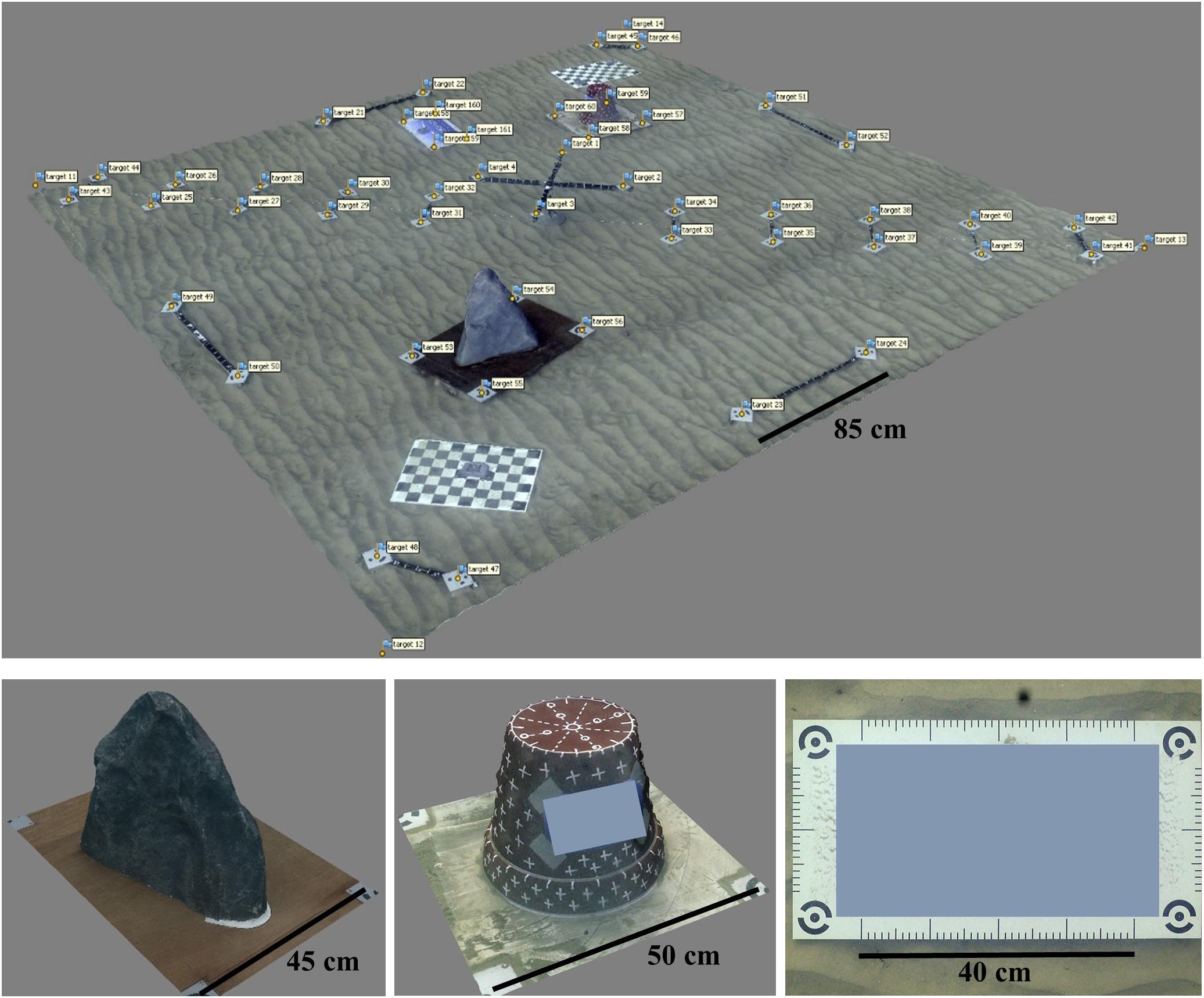
Figure 2. Study site of experiment 2, sub-models of the rock, bucket, and the logo pane, with rulers.

Models Processing and Camera Calibration

All models were processed with Agisoft PhotoScan Professional Edition V. 1.4.0 (Agisoft, 2018). This commercial software is commonly used by the scientific community (Burns et al., 2015a, b, 2016; Figueira et al., 2015; Guo et al., 2016; Casella et al., 2017; Mizuno et al., 2017) and uses a classic photogrammetric workflow. This consists in the automatic identification of key points on all photos, bundle adjustment, point cloud densification, mesh building and texturing. We used the self-calibration procedure implemented in PhotoScan to be as simple and operational as possible, as it has been shown that the refraction effects at the air-port and port-water interfaces can be absorbed by the physical camera calibration parameters during self-calibration (Shortis, 2015). Calibration optimization was conducted for all properties after bundle adjustment (see step 1 in Figure 1).

For the experiment 2, the volume and surface area of the rock and bucket were computed and exported after completing a “hole filling” step to close each sub-model. The models were processed on a Windows 10 workstation with the following specifications: 64bits OS, 128 Gb RAM, 2 × NVIDIA GeForce GTX 1080 Ti 11 Gb, Intel Core i9-7920X 12 CPU 2.9 GHz.

Metrics

Accuracy of Bundle Adjustment

For all processed models, we computed several metrics with a view to assessing the accuracy of bundle adjustment. The reprojection error (see Table 2) is a good indicator of the quality of self-calibration process during bundle adjustment. The Ground Control Point Root Mean Square Error (GCP RMSE) measures the difference between true coordinates of a GCP and its coordinates calculated from all photos. The GCP RMSE/Ground Sample Distance ratio (GSD) gives good indication of the realized vs. potential accuracy (Förstner and Wrobel, 2016), as GSD corresponds to the pixel size in mm (see Table 2). Experiment 1 aims at minimizing these three metrics to ensure accurate bundle adjustment.

TABLE 2

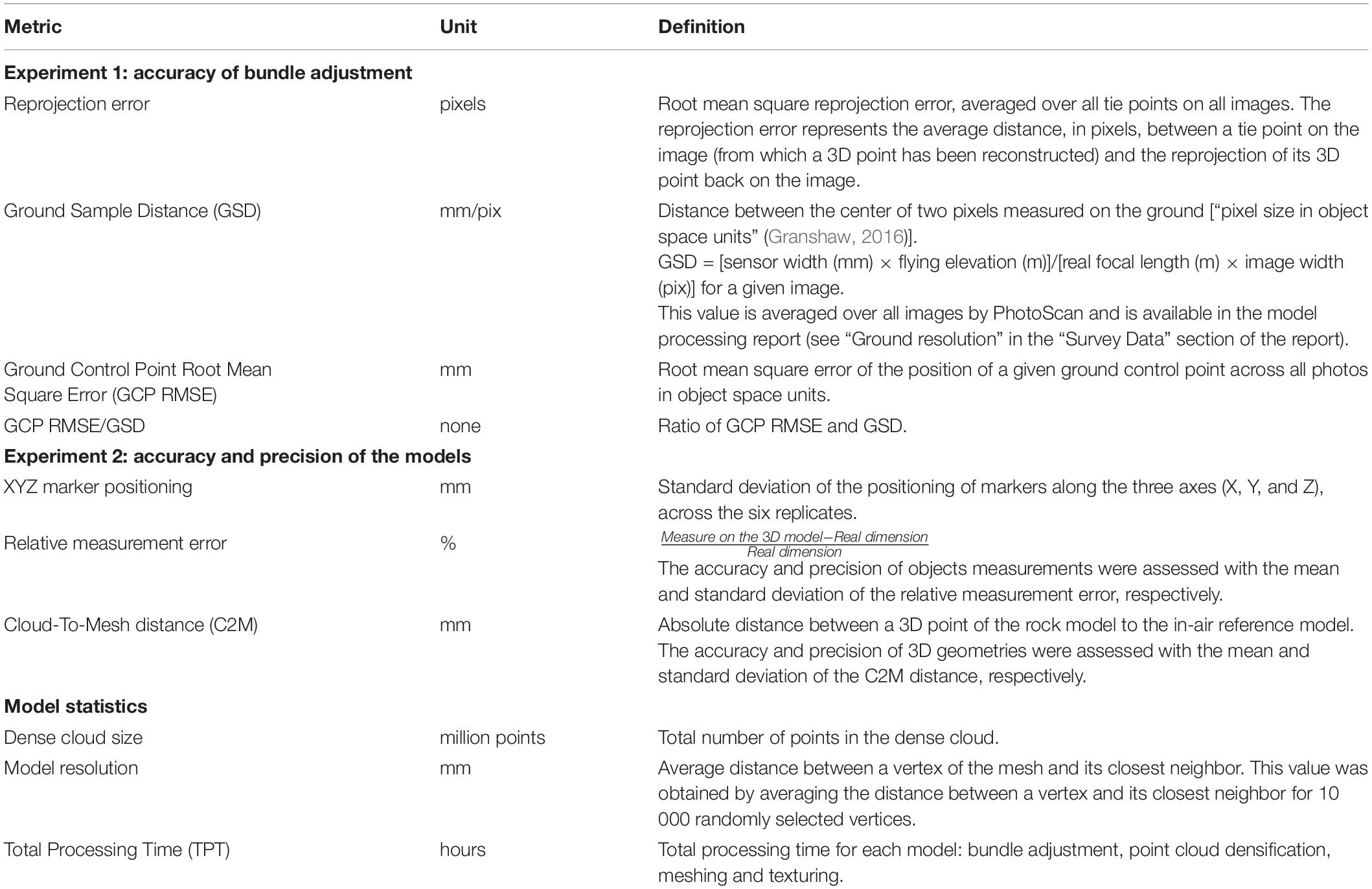
Table 2. Definition of the metrics used in this study.

Model Statistics

Since the aim of this study was to define the best trade-off between the development of high-resolution models and the speed of their reconstruction, model resolution and TPT were computed for all processed models. Model resolution was defined as the average distance between a vertex of the mesh and its closest neighbor (see Table 2), and the TPT including bundle adjustment, point cloud densification, meshing and texturing. In order to take into account model completeness, the dense cloud size (million points) was also calculated.

Accuracy and Precision of the Models

The precision of the positioning of 52 coded markers was assessed by calculating the SD of their XYZ position across the six replicates (see Table 2). The SD was analyzed with regards to the distance to the model center, to assess a potential decrease in precision for points located further away from the center. The accuracy of the positioning was not assessed because exact XYZ positions of the markers was not available.

The accuracy and precision of measurements for all objects of known dimensions (lengths, areas, volumes; see step 4 in Figure 1) were assessed with the mean and SD of the relative measurement error (see Table 2). The simple geometry of the bucket allowed for the calculation of its volume and surface area. The rock volume and surface area were measured on an ultra-high resolution, in-air reconstruction (Bryson et al., 2017) using 255 photographs taken with the Nikon D4. The photos were taken from a variety of orientations, using maximum quality parameters for reconstruction. The in-water rock models were aligned to the in-air reference with the four coded markers, and compared using cloud-to-mesh signed distance implemented in CloudCompare Version 2.10 (CloudCompare, GPL software, 2018). The accuracy and precision of the reconstructions were assessed with the mean and SD of absolute distances between the six replicates and the in-air reference (see Table 2), calculated for 5 000 000 points randomly selected on the reference rock surface.

Analysis of the Results

All marker positions and model statistics were exported from PhotoScan as text and PDF files (PhotoScan processing reports). They were parsed and analyzed with R Software V. 3.4.2 (R Core Team, 2017). The accuracy of bundle adjustment was assessed using the reprojection error, GCP RMSE and GCP RMSE/GSD. The resolution of the models after densification and meshing was defined as the average distance between two neighbor vertices of the mesh (see “Model Statistics”). The individual effect of each parameter (camera system, flying elevation, camera orientation and photo density) on the different metrics (reprojection error, GCP RMSE, GCP RMSE/GSD, dense cloud size, model resolution and TPT) was evaluated with a linear mixed effect model (LMM) (Zuur et al., 2009) after a log-transformation was performed to linearize the relationship with photo density. LMMs are statistical models that are suited for the analysis of clustered dependent data. Indeed, in all models built from the subsampling of one of the 24 datasets from experiment 1 (for studying the effect of photo density on the different metrics) data points are not independent. LMMs incorporate both fixed (the explanatory factors: camera system, flying elevation, camera orientation, photo density) and random effects used to control for pseudo-replication in the data by taking into account heterogeneity in the relationships between the explained variable and explanatory factors among the datasets (Patiño et al., 2013). The random effects structure depicts the nesting of datasets from the most to the least inclusive (camera > flying elevation > orientation > replicate). Models were fit with the “lmer” function in the “lme4” R library (v. 1.1-21). Each LMM was first built with all 4 predictors and sequentially pruned by dropping the least significant predictor until all remaining predictors were significant, such that the final LMMs only included the predictors that had a significant effect on each metric (t-test < 0.05). GSD was independently used as a predictor of the dense cloud size, model resolution and TPT in order to integrate both camera and flying elevation effects and make the results generalizable to a broader range of camera systems and flying elevations.

In experiment 1, the aim was to minimize the reprojection error, the GCP RMSE, the GCP RMSE/GSD, the model resolution, and the TPT, whilst maximizing the dense cloud size. Experiment 2 assessed the accuracy and precision of the reconstructions obtained with the best set of parameters from experiment 1. This was conducted through the analysis of the XYZ positioning of markers, objects lengths, surfaces and volume measurements, and cloud-to-mesh distance between the rock reconstructions and an ultra-high in-air reference model.

Results

The weather conditions were clear during both experiments (swell < 0.5 m, wind < 5 knots), and the sky was cloudy, ensuring homogenous enlightening at those relatively shallow depths. Water conditions were homogenous, and refraction was supposed constant over time and space during acquisition, as it has been proven to be insensitive to temperature, pressure and salinity (Moore, 1976). The total acquisition time for both nadiral and oblique passes was 5 to 7 min for one given combination of parameters (see step 1 in Figure 1). All coded markers were well detected by PhotoScan for all models, and all appeared on a minimum of 4 photos.

Influence of Acquisition Parameters on Bundle Adjustment Accuracy and Model Statistics

Accuracy of Bundle Adjustment

The reprojection error ranged from 0.30 to 0.65 pixels across all models, but was significantly smaller at 2.5 m flying elevation and pure nadiral orientation. The proportion of variance explained for the overall reprojection error was 96.7% (see Table 3). All parameters had a significant effect on the reprojection error (t-test, p < 0.001), except camera system (t-test, p > 0.05).

TABLE 3

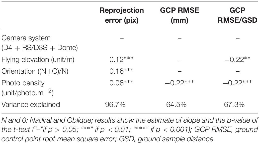
Table 3. Effects of the acquisition parameters on the bundle adjustment metrics.

The GCP RMSE ranged from 0.1 to 9.0 mm across all combinations, but 83 % of models had a value smaller than 1 mm (see Figure 3). The proportion of variance explained for the overall modeled GCP RMSE was 64.5%. The only parameter that had a significant effect on GCP RMSE was the photo density (t-test, p < 0.001, see Table 3), with a negative trend.

FIGURE 3

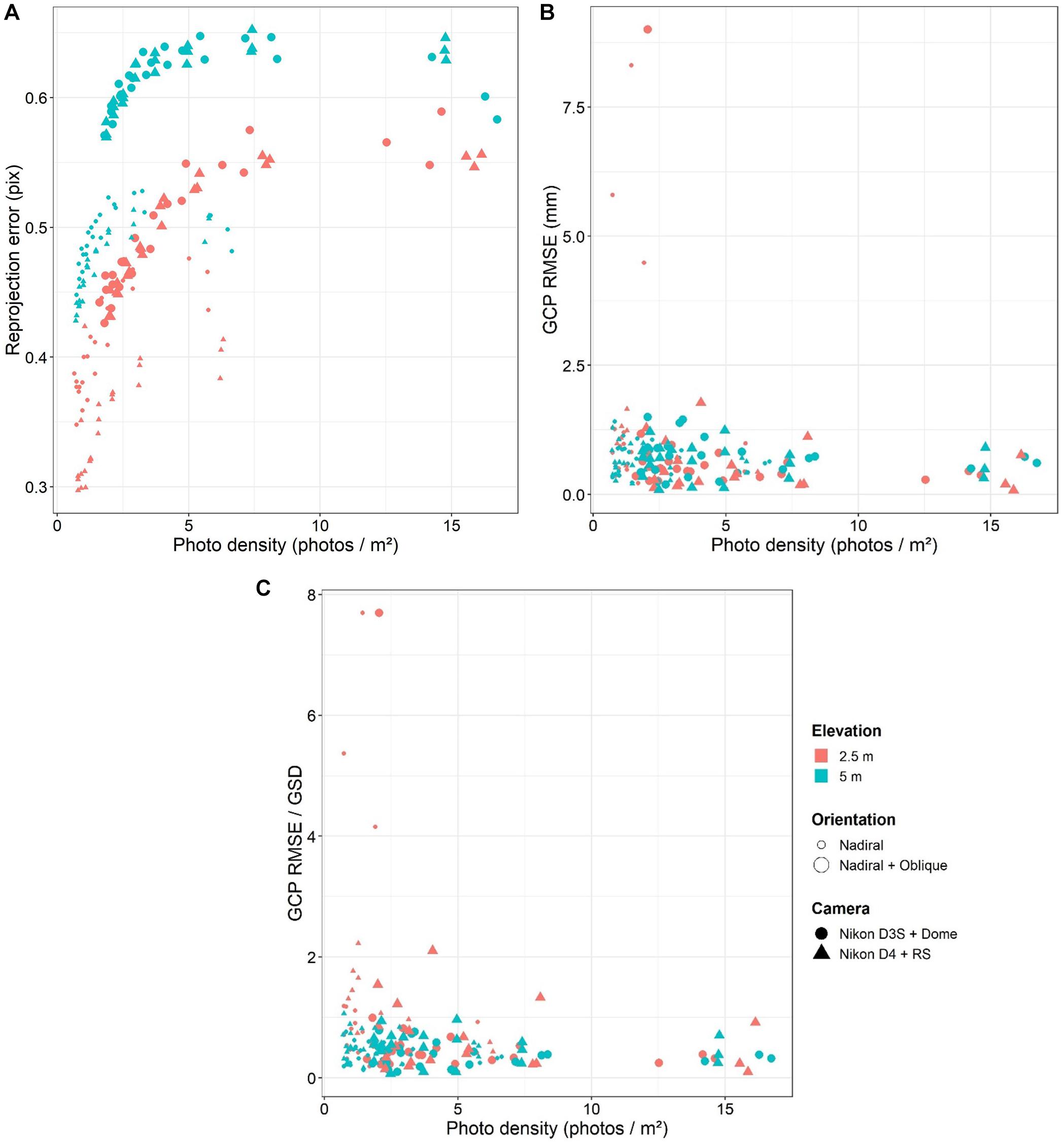
Figure 3. Bundle adjustment metrics in function of the acquisition parameters. (A) Reprojection error; (B) GCP RMSE; and (C) GCP RMSE/GSD ratio; GCP RMSE, ground control point root mean square error; GSD, ground sample distance.

The GCP RMSE/GSD ratio ranged from 0.1 to 7.7 across all combinations, but 89 % of models had a ratio smaller than 1. The proportion of variance explained for the overall modeled GCP RMSE/GSD ratio was 67.3% Both flying elevation and photo density had a significant effect on the GCP RMSE/GSD ratio (t-test, p < 0.01 and p < 0.001, respectively). Camera system and orientation did not have any significant effect (t-test, p > 0.05).

Dense Cloud Size

The dense cloud size ranged from 3.3 to 24.1 million across all models, but was significantly smaller for the Nikon D3S + Dome with 5 m flying elevation and nadiral + oblique orientation (t-test, p < 0.001, See Table 4). The proportion of variance explained for the overall dense cloud size was 99.9%. The camera system and flying elevation accounted for 94.0% of the total variance. The orientation and photo density had a significant effect on the model resolution (t-test, p < 0.001) but only accounted for 5.9% of the total variance. GSD as single predictor had a significant effect (t-test, p < 0.001) and accounted for 78.3% of the total variance. This GSD effect corresponded to about −0.15 to −0.62 million points/m² per mm.pix^–1 (log scale). The combination of parameters that gave the highest dense cloud size included the Nikon D4 + RS with a flying elevation of 2.5 m, and pure nadiral orientation (mean 19.4 million points ± 2.2 SD; see Figure 4).

TABLE 4

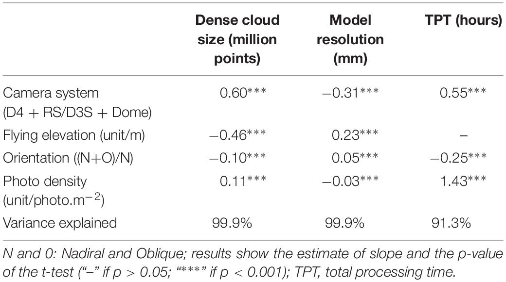
Table 4. Effects of the acquisition parameters on the model statistics.

FIGURE 4

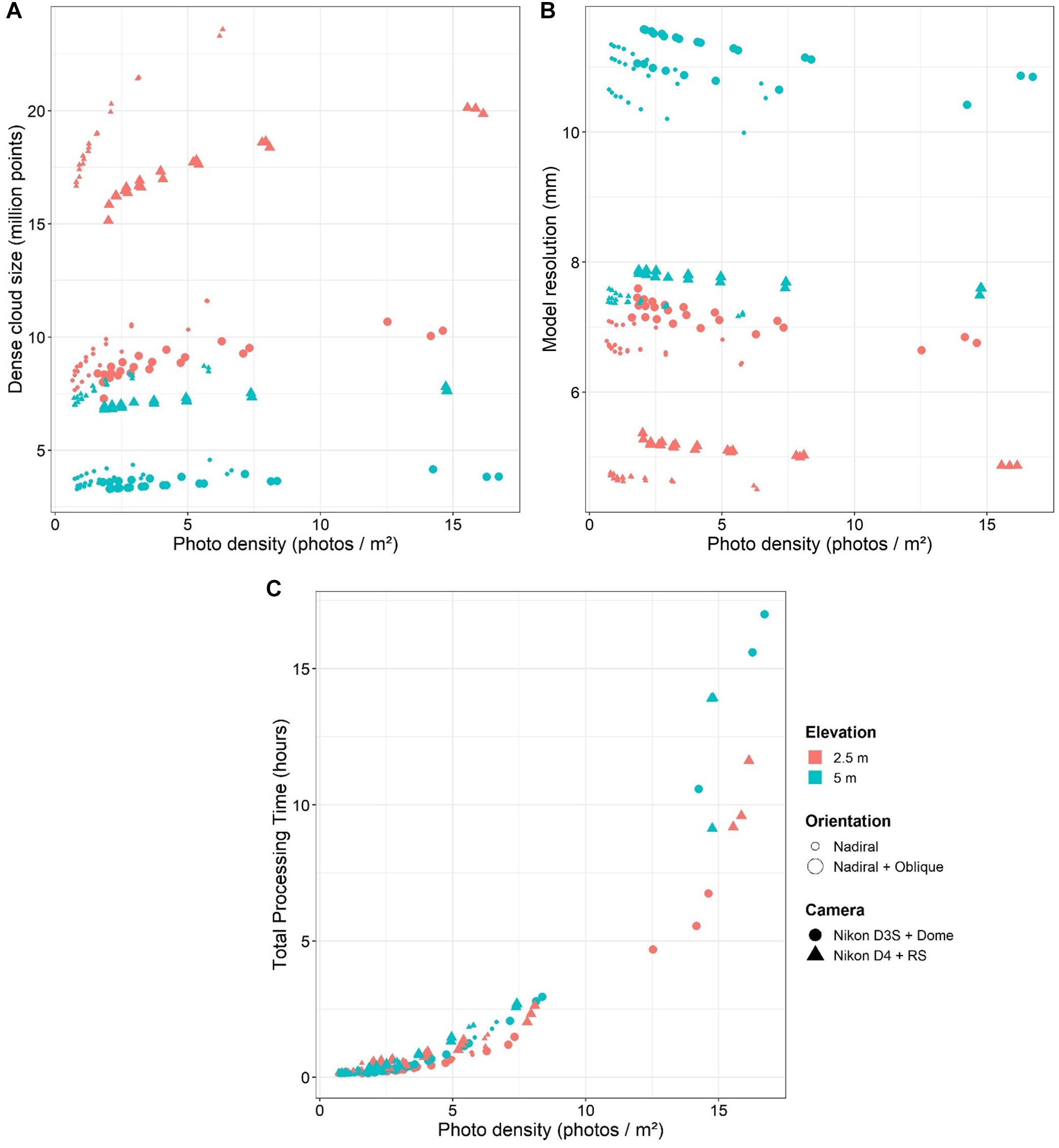
Figure 4. Model statistics in function of the acquisition parameters. (A) Dense cloud size; (B) Model resolution; and (C) Total Processing Time.

The exponential regressions for each combination were in turn calculated (R² = 0.42–0.99). Using the regression curves for each combination, the dense cloud size reached 95% of the maximum value achieved for a photo density between 3.3 and 18.9 photos/m², depending on the camera system, elevation, and orientation. For the stated values of photo density, the dense cloud size was 95% of the maximum value achieved, and additional photos only increased the number by the remaining 5%. The lowest photo density value was obtained from the Nikon D4 + RS camera using pure nadiral orientation at 5 m elevation, while the highest value was obtained from the Nikon D3S + Dome camera using nadiral and oblique orientation at 5 m elevation. The value obtained from the Nikon D4 + RS, 2.5 m altitude and pure nadiral orientation was 4.7 photos/m².

Model Resolution

The model resolution ranged from 4.5 to 11.6 mm across all models but was significantly smaller for the Nikon D4 + RS with 2.5 m flying elevation and nadiral orientation (t-test, p < 0.001, see Table 4). The proportion of variance explained for the overall model resolution was 99.9 %. The camera system and elevation explained 96.8% of the total variance. The orientation and photo density had a significant effect on the model resolution (t-test, p < 0.001) but only accounted for 3.1% of the total variance. GSD as single predictor had a significant effect (t-test, p < 0.001) and accounted for 89.0% of the total variance (with log scale). But GSD and model resolution were linearly positively correlated (Pearson correlation: 0.99), with the following intercept and slope: model resolution = 0.4 + 5.8 mm/mm.pix^–1. The combination of parameters that gave the finest model resolution included the Nikon D4 + RS with a flying elevation of 2.5 m, and pure nadiral orientation (mean 4.6 mm ± 0.06 SD; see Figure 4). Model resolution was highly anti-correlated with the dense cloud size (spearman correlation: −0.98).

Total Processing Time

TPT increased exponentially with the photo density, ranging from 4 min 40 s to 17 h (see Figure 4). TPT was strongly dependent on the photo density, camera system, and orientation (t-test, p < 0.001, see Table 4), with 91.3 % explained variance, but flying elevation was not significant (t-test, p > 0.05). GSD as single predictor did not have any significant effect (t-test, p > 0.05).

Exponential regressions were calculated for each combination (R² = 0.87–0.99). From the regression curves for each combination, it was deduced that the TPT reached a 5% of the overall maximum value for a photo density of 3.8–8 photos/m², depending on the camera system, elevation, and orientation. The lowest photo density values were obtained for Nikon D4 + RS camera at 5 m elevation (for both orientations), while the highest value was obtained for Nikon D3S + Dome camera, pure nadiral orientation and 2.5 m elevation. The value for Nikon D4 + RS at 2.5 m and pure nadiral orientation was 5.0 photos/m².

Accuracy and Precision of the Models With the Best Combination of Parameters

The results stated above show that the best trade-off between high bundle adjustment accuracy, high dense cloud size, high-resolution modeling and low TPT was achieved using the Nikon D4 + RS camera system at a flying elevation of 2.5 m, using pure nadiral orientation and a targeted photo density of 4–5 photos/m² (which corresponds approximately to 1 photo/s at a swimming speed of 20–25 m/min). This combination of parameters was used to assess the quality of the models in experiment 2 (six replicates). The average reached photo density was 4.3 photos/m² ± 0.18 SD over the six datasets with a model resolution of 3.4 mm ± 0.2 SD. GCP RMSE on the four markers of the cross scale bar ranged from 0.76 to 0.93 mm.

Positioning of Markers

The SD of the positioning of 52 markers placed across the modeled area ranged from 0.2 to 1.9 mm in X, 0.2 to 1.8 mm in Y and 0.2 to 4.3 mm in Z (see Figure 5). The SD increased with distance to the model center for all three axes (t-test, p-value < 0.001; see Table 5).

TABLE 5

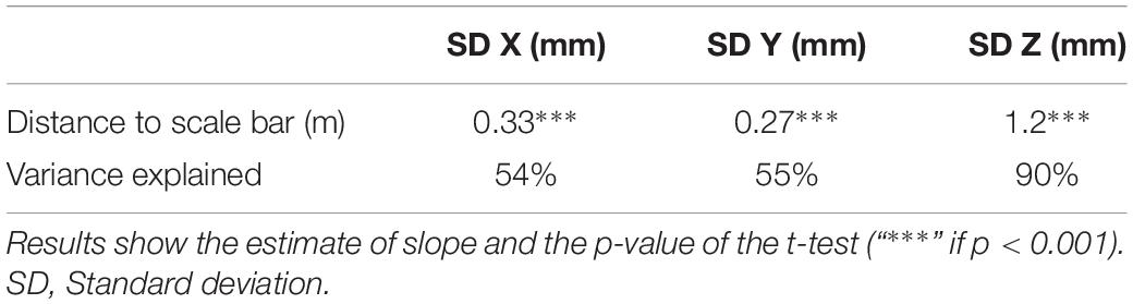
Table 5. Effects of the distance to scale bar on the standard deviation of marker coordinates for the 3 axes.

FIGURE 5

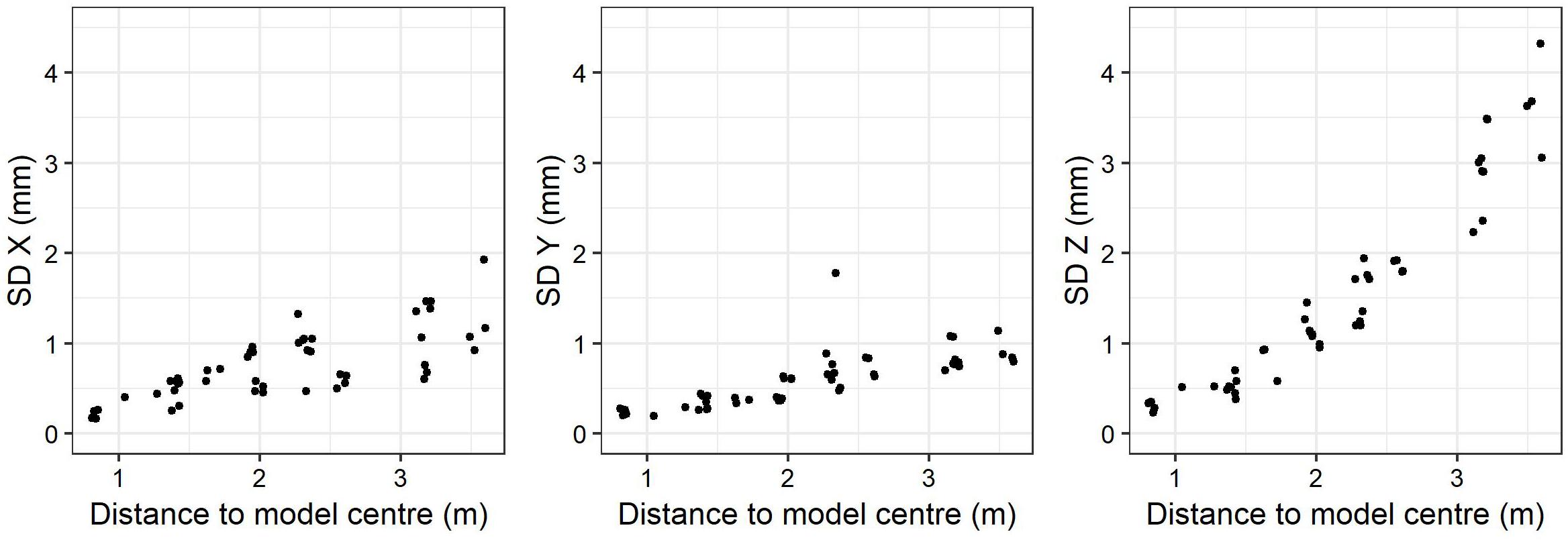
Figure 5. Standard deviation of marker coordinates for the 3 axes, in function of the distance to the model center. SD, standard deviation.

Measures of Lengths, Surfaces and Volumes

The calculation of all measurements was very accurate (mean error < 1%, see Table 6) and precise (SD error < 0.6%), except in the case of describing the bucket’s surface area, which indicated a lower accuracy (mean error = 16.11%) and precision (SD error = 2.12%; see Table 6).

TABLE 6

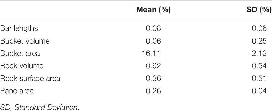
Table 6. Mean and standard deviation of the relative measurement errors for objects contained in the scene (experiment 2).

Reconstruction of 3D Geometries

The in-air model reference of the rock had a resolution of 0.5 mm. The absolute cloud-to-mesh distance between the underwater and the in-air rock model, computed on 5 000 000 randomly selected points, ranged from 0.04 to 9.6 mm across the six replicates (see Figure 6). The mean absolute C2M distance over all points and all replicates was 1.2 mm. The SD of the absolute C2M distance across the six replicates ranged from 0.01 to 9.5 mm, with a mean value over all points of 0.8 mm. Mean and SD of C2M distance were highly correlated (spearman correlation: 0.77).

FIGURE 6

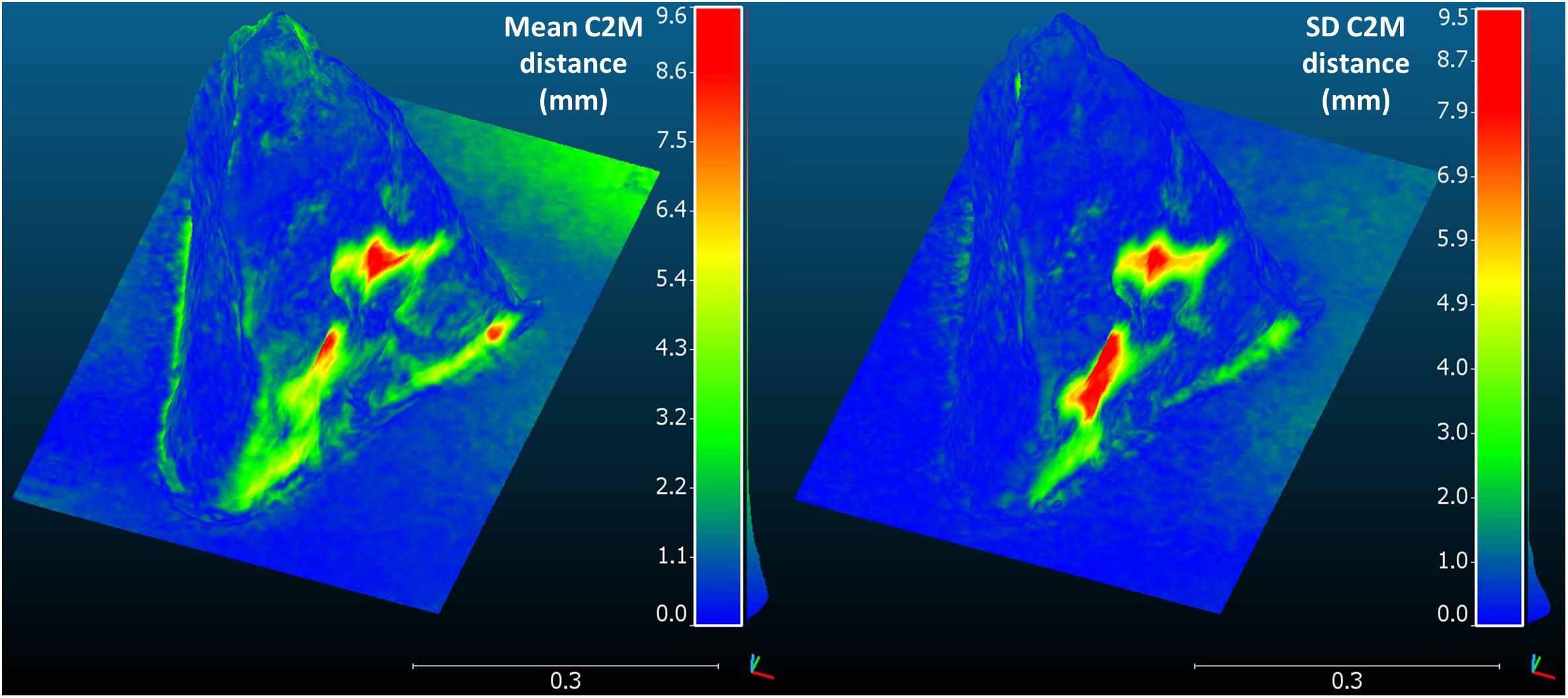
Figure 6. Mean and standard deviation of the absolute cloud-to-mesh distance between the six replicates of the rock model and the in-air reference model. C2M, cloud-to-mesh; SD, standard deviation.

Discussion

This study aimed at developing a simple and operational methodology for the 3D reconstruction of marine habitats, with the highest resolution, accuracy and precision, for the shortest processing time. We evaluated the effects of the camera system, flying elevation, camera orientation, and photo density on the resulting reconstructions of a 6 × 6 m sand patch using reprojection error, GCP RMSE, model resolution, and TPT. By considering the parameters which gave the best results, and the photo density which achieved the best trade-off between accuracy of the reconstructions and processing time, this study assessed the expected accuracy and precision of reconstructions on a second study site with reference objects of known dimensions and geometry.

Best Practices for Underwater Photogrammetry

The bundle adjustment was mostly accurate across all combinations, with a reprojection error no greater than 0.65 pixels and a GCP RMSE/GSD ratio smaller than one for 89% of the models. This ratio is a good indicator as it represents the ratio between realized and potential accuracy (Förstner and Wrobel, 2016). It was smaller at higher photo densities, indicating that photo density gives more robustness during bundle adjustment. The reprojection error increased with photo density (t-test, p-value < 0.001), but there was a saturation point around 5–7 photos/m² with a lower slope for higher densities. Indeed, the reprojection error naturally increases at low photo densities, as with very few photos it is expected that 3D points are reconstructed from only 2–3 images and thus have a null or low reprojection error. Flying elevation and nadiral + oblique orientation showed higher reprojection error, due to a lower sharpness of images taken in these configurations. The camera system did not have any significant effect on the reprojection error, which suggests that the self-calibration algorithm implemented in PhotoScan interpreted and corrected the distortions of the two different optical systems fairly successfully. Also, reprojection error is not affected by the sensor resolution as it is expressed in pixel unit.

The two main drivers of model resolution were the camera system and the flying elevation. The model resolution was in average 2.4 mm smaller for the Nikon D4 + RS (log scale), and 1.8 mm/m elevation. By definition, the GSD is directly depending on the resolution and size of the camera sensor, and distance to modeled object (Förstner and Wrobel, 2016). Therefore, the closer to the object and the higher the resolution of the sensor, the smaller the GSD. Model resolution and GSD being highly linearly correlated (Pearson correlation: 0.99), a smaller GSD involves a smaller model resolution. Its effect corresponded to 5.8 mm/mm.pix^–1 (any increase in GSD by 1 mm leads to an increase of 5.8 mm in model resolution, with quality setting for the dense cloud set to “high”). This is an interesting result to keep in mind when planning a photogrammetric acquisition, as GSD can be calculated from sensor properties and flying elevation (see Table 2). For a desired model resolution and a given camera system, one can estimate the corresponding flying elevation to be practiced. However, the quality of the camera system will condition the best possible model resolution, as decreasing the flying elevation would require more and more photos to maintain sufficient overlap between pictures, in turn increasing the overall processing time. Other unpublished experiments undertaken by the participants of this study confirm the impracticality of further decreasing flying elevation in the case of homogenous textures such as muddy sediment or dense seagrass, since the footprints of photos taken at lower elevation can be too small to ensure the reliable capture of key points, confusing the bundle adjustment algorithm. This issue was not observed in the case of biogenic reefs such as coralligenous or coral reefs that exhibit a high number of reliable key points.

On the other hand, dense cloud size was highly anti-correlated with model resolution (spearman correlation: −0.98), hence affected by the same parameters as model resolution, with reverse trends. Indeed, the model resolution was here defined as the average distance between a vertex of the mesh and its closest neighbor. But at low photo densities, the dense cloud size was also impacted by missing surfaces that could not be reconstructed because of the insufficient coverage (mostly at the model edges). This was not observed for photo densities greater than 3–4 photos/m². Taking this effect into account by normalizing by the total area, GSD had an effect of about −0.15 to −0.62 million points/m² per mm.pix^–1 (log scale; any increase in GSD by 1 mm.pix^–1 leads to a decrease of 0.15 to 0.62 million points per square meter).

The camera orientation significantly influenced most of the metrics, but most importantly affected the reprojection error. All analyses showed that the best results could be obtained by using pure nadiral orientation rather than nadiral and oblique orientation, contrary to the findings of other studies (Chiabrando et al., 2017). It is nevertheless important to underline the fact that, whilst the selected study sites had a relatively flat topography with low-height objects, in the case of more complex environments such as reefs, oblique images can be vitally important to ensuring the comprehensive analysis of all details of the site. This is illustrated by the cloud-to-mesh distances represented in Figure 6: the lowest accuracy and precision corresponded to points located below overhanging parts of the rock that were not always well-represented by the photographs, depending on the exact position of each photo.

TPT exponentially increased with photo density, necessitating a trade-off between accurate bundle adjustment/high dense cloud size and expected TPT. It was concluded that a value of 4–5 photos/m² of mapped seafloor worked well at 2.5 m height. A higher number of photos would mean that the TPT would have been considerably higher whilst the accuracy of bundle adjustment and dense cloud size would have seen no such corresponding increase. With 16.2 Mpix, the Nikon D4 required a significantly higher TPT than the Nikon D3S and its 12.1 Mpix sensor, but this effect was marginal compared to the one of photo density (see Table 4).

The workflow designed in this study used “high” quality setting for dense cloud generation (see Figure 1), which corresponds to a downscaling of the original image size by factor of four [two times by each side, (Agisoft, 2018)]. However, with this quality level, depth maps and dense cloud generation are the two most time consuming steps of model production (70–80% of TPT). A “medium” quality corresponds to a downscaling of the original image size by factor of 16 (four times by each side) and could drastically reduce TPT. According to the size of the area to be modeled, there could be a trade-off between the GSD (through flying elevation and sensor properties) and the dense cloud quality in order to reach the desired resolution within the shortest TPT. At low flying elevation, more photos are required to cover the area, but the GSD is smaller, which might not require the same quality level as a higher flying elevation in order to reach a given model resolution. Further investigations should tackle this point to help researchers making decisions on this trade-off.

Accuracy and Precision of the Resulting Methodology

The positioning of markers in the scene was achieved with a SD smaller than 5 mm on the three axes, but was increasing with distance to the center at a rate of about 0.3 mm/m in XY and 1.2 mm/m in Z. If this precision can be sufficient in many usages, it must be taken into consideration notably in the case of model comparison, such as coral or coralligenous outcrops growth at a reef scale. For such applications, the model should always be centered on the area requiring the finest precision, and changes in Z must be larger than the precision expected at the given distance to reflect true reef changes or growth. This underlines the need for further study at a broader scale so as to evaluate the decrease in precision for areas > 100 m². People using underwater photogrammetry can place coded markers at the boundaries of the region of interest to assess the lowest expected precision of their models, especially on the Z axis.

However, the methodology achieved a satisfactory accuracy for length measurements, with measurement errors corresponding to 8.0 mm per 10 m. It is important to note that the reference bars used were only 0.35 to 0.85 m long and that the accuracy could be different at larger scales. With regards to volumes and surfaces, the expected accuracy was predicted to decrease with increased object complexity, as informed by several studies (Figueira et al., 2015; Bryson et al., 2017). The poorest accuracy and precision occurred in the calculation of the bucket’s surface area. It is quite possible that the texture was too homogenous and that PhotoScan could not identify enough tie points on the surface to build its shape, resulting in important surface artifacts. This must be taken into consideration when monitoring artificial structures with very poor texture such as newly submerged metallic or concrete structures. The reconstruction of the resin-made rock (an imitation of natural surfaces and shapes) on the other hand proved to be very accurate (0.92% error for volume and 0.36% for area) and precise (0.54% SD for volume and 0.51% for area), surpassing previous results in similar studies (Bythell et al., 2001; Courtney et al., 2007; Figueira et al., 2015; Lavy et al., 2015; Shortis, 2015; Gutierrez-Heredia et al., 2016). Comparing 3D meshes, the models were also very accurate and precise with a mean C2M distance of 1.2 mm over 5 000 000 randomly selected points on the rock surface, and a SD of 0.8 mm over the six replicates. The highest differences with the in-air reference model were observed for points below overhanging parts of the rock (see Figure 6), as they were not always captured by the pure nadiral photos. The highest variability was observed for the same points. Indeed, according to the exact position of photos for each dataset, these points were accurately reconstructed for some replicates, and showed artifacts for others. This highlights the limits of pure nadiral orientation in the case of more complex structures, where the operator should adapt camera orientation to follow the structure of the modeled object.

With the exception of the calculated surface of the bucket, the methodology produced highly accurate and precise reconstructions. The method is well-suited and easily deployed for the study and monitoring of marine benthic ecosystems. Using this method, artificial or natural habitats that exhibit the same level of complexity as the experimental setup (low complexity) could be monitored with an expected 1.2 mm accuracy. Healthy biogenic habitats such as coralligenous and coral reefs are expected to show a high complexity; the accuracy of the method still needs to be assessed for these habitats, as reconstruction errors are known to increase with habitat complexity (Figueira et al., 2015; Bryson et al., 2017). This solution is cost-effective and operational in terms of the material resources required for monoscopic photogrammetry, time required underwater, and post-processing time. By comparison, whilst stereoscopic mounts enable the direct scaling of the scene (Ahmadabadian et al., 2013), they cost twice as much as monoscopic cameras, produce twice as many photos increasing the overall processing time, and do not necessarily achieve more accurate results (Abdo et al., 2006; Figueira et al., 2015; Bryson et al., 2017).

Integration of This Method Within Marine Ecosystem Monitoring Networks

Photogrammetry has been increasingly used for studying and monitoring marine biodiversity (as aforementioned in the introduction). It has been deemed a suitable tool for monitoring natural or anthropogenic disturbances and their effects on biodiversity in marine ecosystems (Burns et al., 2016). The results of this study showed that, at the small reef scale, photogrammetry can provide very accurate and precise sub-centimetric reconstructions.

Biogenic reefs and seagrass meadows are two of the most frequently monitored marine habitats because of the ecological role they play for biodiversity (Ballesteros, 2006; Boudouresque et al., 2012; Coker et al., 2014). Photogrammetry is particularly well suited for the monitoring of reefs as they are built of sessile and immobile organisms, and their 3D structure is known to play a major role in structuring their constitutive ecological assemblages (see introduction). However, artificial light becomes mandatory over 30–40 m depth because of light absorption, notably in the case of deeper habitats such as coralligenous reefs (Ballesteros, 2006). The methodology outlined by this study can be used to monitor small to medium size reefs (20–500 m²); to characterize their structural complexity, measure growth rates and study 3D relationships between species, for example. Given recent developments in deep learning, third-dimensional models can be exploited as an additional information layer for classifying species from their 3D characteristics (Maturana and Scherer, 2015; Qi et al., 2016). Models of sub-centimetric resolution are currently confined to use on a small area for practical reasons and computational limitations, but future technological advances might enable use on larger extents. Future research should focus on the use of photogrammetric technology in developing scientific understanding of complex ecological processes related to structure. In the coming years, photogrammetry should support detailed studies covering vast marine regions, opening opportunities to draw correlations with macroecological variables available at a broader scale.

Conclusion

There has been an increasing demand in recent years for innovative methods capable of easily and efficiently capturing fine-scale ecological processes and detecting small changes for the monitoring of the effects of anthropogenic pressures on marine habitats. This study outlined a method that enables the production of accurate and reproducible, high-resolution models of marine environments with a low TPT. The simple experimental design supported the test of a set of variables proven operational. All in all, the method is suitable for the monitoring of marine benthic biodiversity in a large-scale multi-sites monitoring system. The study’s results showed that flying elevation and camera system, and therefore GSD, strongly affected the model resolution. Photo density meanwhile vastly influenced processing time and bundle adjustment accuracy. If the operator effect was not studied here, because it indirectly accounts for several factors that are not straightforward (i.e., trajectory, flying elevation, camera orientation, swimming speed, etc.), it should be tackled as it could have a major influence, notably at large scales. Accounting for computing limitations, future investigations should assess the accuracy and precision of models built with the same parameters, but at a larger scale (>500 m²). The influence of the dense cloud quality setting should also be studied as it is expected to play an important role the trade-off between model resolution and TPT. This study was necessary prior to ecological interpretations of 3D models built with the resulting methodology.

Data Availability

The datasets generated for this study are available on request to the corresponding author.

Author Contributions

GM, JD, and FH designed the study and collected the data; GM produced the 3D models and performed the statistical analysis; GM, JD, SL, and PB contributed to the results interpretation; GM wrote the first draft of the manuscript and produced the figures; JD and SL supervised the research project. All authors contributed to manuscript revision, read and approved the submitted version.

Funding

This study beneficiated from a financing of the French Water Agency (Agence de l’eau Rhône-Méditerranée-Corse) (convention n° 2017-1118) and the LabCom InToSea (ANR Labcom 2, Université de Montpellier UMR 9190 MARBEC/Andromède Océanologie). GM received a Ph.D. grant (2017–2020) funded by Agence Nationale pour la Recherche Technologique (ANRT) and Andromède Océanologie.

Conflict of Interest Statement

The authors declare that the research was conducted in the absence of any commercial or financial relationships that could be construed as a potential conflict of interest.

Acknowledgments

We thank the STARESO marine station for their hospitality and help for the fieldwork in Calvi bay, and Antonin Guilbert (Andromède Océanologie) for his help in setting up the 2nd experiment in Roquebrune. The two acquisition phases were possible thanks to the logistic support of Andromède Océanologie and the French Water Agency during the annual fieldwork campaign of TEMPO and RECOR monitoring networks (http://www.medtrix.fr/). Many thanks to François Guilhaumon for his advices on the mixed effect models, and to the two reviewers for their relevant comments and suggestions.

References

Abdo, D. A., Seager, J. W., Harvey, E. S., McDonald, J. I., Kendrick, G. A., and Shortis, M. R. (2006). Efficiently measuring complex sessile epibenthic organisms using a novel photogrammetric technique. J. Exp. Mar. Biol. Ecol. 339, 120–133. doi: 10.1016/j.jembe.2006.07.015

CrossRef Full Text | Google Scholar

Agisoft (2018). Agisoft PhotoScan User Manual: Professional Edition, Version 1.4. 127.

Google Scholar

Agudo-Adriani, E. A., Cappelletto, J., Cavada-Blanco, F., and Croquer, A. (2016). Colony geometry and structural complexity of the endangered species acropora cervicornis partly explains the structure of their associated fish assemblage. PeerJ 4:e1861. doi: 10.7717/peerj.1861

PubMed Abstract | CrossRef Full Text | Google Scholar

Ahmadabadian, A. H., Robson, S., Boehm, J., Shortis, M., Wenzel, K., and Fritsch, D. (2013). A comparison of dense matching algorithms for scaled surface reconstruction using stereo camera rigs. ISPRS J. Photogramm. Remote Sens. 78, 157–167. doi: 10.1016/j.isprsjprs.2013.01.015

CrossRef Full Text | Google Scholar

Ballesteros, E. (2006). Mediterranean coralligenous assemblages: a synthesis of present knowledge. Oceanogr. Mar. Biol. 44, 123–195. doi: 10.1201/9781420006391.ch4

CrossRef Full Text | Google Scholar

Boudouresque, C. F., Bernard, G., Bonhomme, P., Charbonnel, E., Diviacco, G., Meinesz, A., et al. (2012). Protection and Conservation of Posidonia Oceanica Meadows. Tunis: RAMOGE and RAC/SPA publisher, 1–202.

Google Scholar

Bryson, M., Ferrari, R., Figueira, W., Pizarro, O., Madin, J., Williams, S., et al. (2017). Characterization of measurement errors using structure-from-motion and photogrammetry to measure marine habitat structural complexity. Ecol. Evol. 7, 5669–5681. doi: 10.1002/ece3.3127

PubMed Abstract | CrossRef Full Text | Google Scholar

Burns, J. H. R., Delparte, D., Gates, R.D., and Takabayashi, M. (2015a). Integrating structure-from-motion photogrammetry with geospatial software as a novel technique for quantifying 3D ecological characteristics of coral reefs. PeerJ 3:e1077. doi: 10.7717/peerj.1077

PubMed Abstract | CrossRef Full Text | Google Scholar

Burns, J. H. R., Delparte, D., Gates, R. D., and Takabayashi, M. (2015b). Utilizing underwater three-dimensional modeling to enhance ecological and biological studies of coral reefs. Int. Arch. Photogramm. Remote Sens. Spat. Inform. Sci. XL-5/W5, 61–66. doi: 10.5194/isprsarchives-XL-5-W5-61-2015

CrossRef Full Text | Google Scholar

Burns, J. H. R., Delparte, D., Kapono, L., Belt, M., Gates, R. D., and Takabayashi, M. (2016). Assessing the impact of acute disturbances on the structure and composition of a coral community using innovative 3D reconstruction techniques. Methods Oceanogr. 15–16, 49–59. doi: 10.1016/j.mio.2016.04.001

CrossRef Full Text | Google Scholar

Bythell, J. C., Pan, P., and Lee, J. (2001). Three-dimensional morphometric measurements of reef corals using underwater photogrammetry techniques. Coral Reefs 20, 193–199. doi: 10.1007/s003380100157

CrossRef Full Text | Google Scholar

Casella, E., Collin, A., Harris, D., Ferse, S., Bejarano, S., Parravicini, V., et al. (2017). Mapping coral reefs using consumer-grade drones and structure from motion photogrammetry techniques. Coral Reefs 36, 269–275. doi: 10.1007/s00338-016-1522-0

CrossRef Full Text | Google Scholar

Chiabrando, F., Lingua, A., Maschio, P., and Teppati Losè, L. (2017). The influence of flight planning and camera orientation in UAVs photogrammetry. A Test Area of Rocca San Silvestro (LI), Tuscany. Inte. Arch. Photogramm. Remote Sens. Spat. Inform. Sci. XLII-2/W3, 163–170. doi: 10.5194/isprs-archives-XLII-2-W3-163-2017

CrossRef Full Text | Google Scholar

Chong, A. K., and Stratford, P. (2002). Underwater digital stereo-observation technique for red hydrocoral study. Photogramm. Eng. Remote Sens. 68, 745–751.

Google Scholar

Cocito, S., Sgorbini, S., Peirano, A., and Valle, M. (2003). 3-D reconstruction of biological objects using underwater video technique and image processing. J. Exp. Mar. Biol. Ecol. 297, 57–70. doi: 10.1016/S0022-0981(03)00369-1

CrossRef Full Text | Google Scholar

Coker, D. J., Wilson, S. K., and Pratchett, M. S. (2014). Importance of live coral habitat for reef fishes. Rev. Fish Biol. Fish. 24, 89–126. doi: 10.1007/s11160-013-9319-5

CrossRef Full Text | Google Scholar

Courtney, L. A., Fisher, W. S., Raimondo, S., Oliver, L. M., and Davis, W. P. (2007). Estimating 3-dimensional colony surface area of field corals. J. Exp. Mar. Biol. Ecol. 351, 234–242. doi: 10.1016/j.jembe.2007.06.021

CrossRef Full Text | Google Scholar

Darling, E. S., Graham, N. A. J., Januchowski-Hartley, F. A., Nash, K. L., Pratchett, M. S., and Wilson, S. K. (2017). Relationships between structural complexity, coral traits, and reef fish assemblages. Coral Reefs 36, 561–575. doi: 10.1007/s00338-017-1539-z

PubMed Abstract | CrossRef Full Text | Google Scholar

Dornelas, M., Gotelli, N. J., McGill, B., Shimadzu, H., Moyes, F., Sievers, C., et al. (2014). Assemblage time series reveal biodiversity change but not systematic loss. Science 344, 296–299. doi: 10.1126/science.1248484

PubMed Abstract | CrossRef Full Text | Google Scholar

Drap, P. (2012). “Underwater Photogrammetry for Archaeology,” in Special Applications of Photogrammetry, ed. P. Carneiro Da Silva (Rijeka: InTech), 111–136. doi: 10.5772/33999

CrossRef Full Text | Google Scholar

Dustan, P., Doherty, O., and Pardede, S. (2013). Digital reef rugosity estimates coral reef habitat complexity. PLoS One 8:e57386. doi: 10.1371/journal.pone.0057386

PubMed Abstract | CrossRef Full Text | Google Scholar

Ferrari, R., Bryson, M., Bridge, T., Hustache, J., Williams, S. B., Byrne, M., et al. (2016). Quantifying the response of structural complexity and community composition to environmental change in marine communities. Glob. Change Biol. 22, 1965–1975. doi: 10.1111/gcb.13197

PubMed Abstract | CrossRef Full Text | Google Scholar

Figueira, W., Ferrari, R., Weatherby, E., Porter, A., Hawes, S., and Byrne, M. (2015). Accuracy and precision of habitat structural complexity metrics derived from underwater photogrammetry. Remote Sens. 7, 16883–16900. doi: 10.3390/rs71215859

CrossRef Full Text | Google Scholar

Förstner, W., and Wrobel, B. P. (2016). Photogrammetric Computer Vision: Statistics, Geometry Orientation and Reconstruction. Cham: Springer International Publishing, doi: 10.1007/978-3-319-11550-4

CrossRef Full Text | Google Scholar

Friedlander, A., Sladek Nowlis, J., Sanchez, J. A., Appeldoorn, R., Usseglio, P., Mccormick, C., et al. (2003). Designing effective marine protected areas in seaflower biosphere reserve, colombia, based on biological and sociological information. Conserv. Biol. 17, 1769–1784. doi: 10.1111/j.1523-1739.2003.00338.x

CrossRef Full Text | Google Scholar

Friedman, A., Pizarro, O., Williams, S. B., and Johnson-Roberson, M. (2012). Multi-scale measures of rugosity, slope and aspect from benthic stereo image reconstructions. PLoS One 7:e50440. doi: 10.1371/journal.pone.0050440

PubMed Abstract | CrossRef Full Text | Google Scholar

Garrabou, J., and Ballesteros, E. (2000). Growth of mesophyllum alternans and lithophyllum frondosum (Corallinales, Rhodophyta) in the Northwestern Mediterranean. Eur. J. Phycol. 35, 1–10. doi: 10.1080/09670260010001735571

CrossRef Full Text | Google Scholar

González-Rivero, M., Beijbom, O., Rodriguez-Ramirez, A., Holtrop, T., González-Marrero, Y., Ganase, A., et al. (2016). Scaling up ecological measurements of coral reefs using semi-automated field image collection and analysis. Remote Sens. 8:30. doi: 10.3390/rs8010030

CrossRef Full Text | Google Scholar

González-Rivero, M., Bongaerts, P., Beijbom, O., Pizarro, O., Friedman, A., Rodriguez-Ramirez, A., et al. (2014). The catlin seaview survey - kilometre-scale seascape assessment, and monitoring of coral reef ecosystems. Aquat. Conserv. Mar. Freshw. Ecosyst. 24, 184–198. doi: 10.1002/aqc.2505

CrossRef Full Text | Google Scholar

Graham, N. A. J., and Nash, K. L. (2013). The importance of structural complexity in coral reef ecosystems. Coral Reefs 32, 315–326. doi: 10.1007/s00338-012-0984-y

CrossRef Full Text | Google Scholar

Granshaw, S. I. (2016). Photogrammetric terminology: third edition. The Photogramm. Rec. 31, 210–251. doi: 10.1111/phor.12146

CrossRef Full Text | Google Scholar

Guo, T., Capra, A., Troyer, M., Gruen, A., Brooks, A. J., Hench, J. L., et al. (2016). Accuracy assessment of underwater photogrammetric three dimensional modelling for coral reefs. Int. Arch. Photogramm. Remote Sens. Spat. Inform. Sci. XLI-B5, 821–828. doi: 10.5194/isprsarchives-XLI-B5-821-2016

CrossRef Full Text | Google Scholar

Gutierrez-Heredia, L., Benzoni, F., Murphy, E., and Reynaud, E. G. (2016). End to end digitisation and analysis of three-dimensional coral models, from communities to corallites. PLoS One 11:e0149641. doi: 10.1371/journal.pone.0149641

PubMed Abstract | CrossRef Full Text | Google Scholar

Gutiérrez-Heredia, L., D’Helft, C., and Reynaud, E. G. (2015). Simple methods for interactive 3D modeling, measurements, and digital databases of coral skeletons: simple methods of coral skeletons. Limnol. Oceanogr. Methods 13, 178–193. doi: 10.1002/lom3.10017

CrossRef Full Text | Google Scholar

Halpern, B. S., Walbridge, S., Selkoe, K. A., Kappel, C. V., Micheli, F., D’Agrosa, C., et al. (2008). A global map of human impact on marine ecosystems. Science 319, 948–952. doi: 10.1126/science.1149345

PubMed Abstract | CrossRef Full Text | Google Scholar

Holmes, G. (2008). Estimating three-dimensional surface areas on coral reefs. J. Exp. Mar. Biol. Ecol. 365, 67–73. doi: 10.1016/j.jembe.2008.07.045

CrossRef Full Text | Google Scholar

Johnson-Roberson, M., Pizarro, O., Williams, S. B., and Mahon, I. (2010). Generation and visualization of large-scale three-dimensional reconstructions from underwater robotic surveys. J. Field Robot. 27, 21–51. doi: 10.1002/rob.20324

CrossRef Full Text | Google Scholar

Kovalenko, K. E., Thomaz, S. M., and Warfe, D. M. (2012). Habitat complexity: approaches and future directions. Hydrobiologia 685, 1–17. doi: 10.1007/s10750-011-0974-z

CrossRef Full Text | Google Scholar

Lavy, A., Eyal, G., Neal, B., Keren, R., Loya, Y., and Ilan, M. (2015). A quick, easy and non-intrusive method for underwater volume and surface area evaluation of benthic organisms by 3D computer modelling. Methods Ecol. Evol. 6, 521–531. doi: 10.1111/2041-210X.12331

CrossRef Full Text | Google Scholar

Leon, J. X., Roelfsema, C. M., Saunders, M. I., and Phinn, S. R. (2015). Measuring coral reef terrain roughness using ‘Structure-from-Motion’ close-range photogrammetry. Geomorphology 242, 21–28. doi: 10.1016/j.geomorph.2015.01.030

CrossRef Full Text | Google Scholar

Maturana, D., and Scherer, S. (2015). “VoxNet: A 3D Convolutional Neural Network for Real-Time Object Recognition,” in Proceedings of the 2015 IEEE/RSJ International Conference on Intelligent Robots and Systems (IROS), (Hamburg: IEEE), 922–928. doi: 10.1109/IROS.2015.7353481

CrossRef Full Text | Google Scholar

McGill, B. J., Dornelas, M., Gotelli, N. J., and Magurran, A. E. (2015). Fifteen forms of biodiversity trend in the anthropocene. Trends Ecol. Evol. 30, 104–113. doi: 10.1016/j.tree.2014.11.006

PubMed Abstract | CrossRef Full Text | Google Scholar

Menna, F., Nocerino, E., and Remondino, F. (2017). “Optical Aberrations in Underwater Photogrammetry with Flat and Hemispherical Dome Ports,” in Proceedings of the SPIE, Italy.

Google Scholar

Mizuno, K., Asada, A., Matsumoto, Y., Sugimoto, K., Fujii, T., Yamamuro, M., et al. (2017). A simple and efficient method for making a high-resolution seagrass map and quantification of dugong feeding trail distribution: a field test at mayo bay, Philippines. Ecol. Inform. 38, 89–94. doi: 10.1016/j.ecoinf.2017.02.003

CrossRef Full Text | Google Scholar

Moore, E. J. (1976). Underwater photogrammetry. Photogramm. Rec. 8, 748–763. doi: 10.1111/j.1477-9730.1976.tb00852.x

CrossRef Full Text | Google Scholar

Patiño, J., Guilhaumon, F., Whittaker, R. J., Triantis, K. A., Robbert Gradstein, S., Hedenäs, L., et al. (2013). Accounting for data heterogeneity in patterns of biodiversity: an application of linear mixed effect models to the oceanic island biogeography of spore-producing plants. Ecography 36, 904–913. doi: 10.1111/j.1600-0587.2012.00020.x

CrossRef Full Text | Google Scholar

Pimm, S. L., Jenkins, C. N., Abell, R., Brooks, T. M., Gittleman, J. L., Joppa, L. N., et al. (2014). The biodiversity of species and their rates of extinction, distribution, and protection. Science 344, 1246752/1–1246752/10. doi: 10.1126/science.1246752

PubMed Abstract | CrossRef Full Text | Google Scholar

Pizarro, O., Friedman, A., Bryson, M., Williams, S. B., and Madin, J. (2017). A simple, fast, and repeatable survey method for underwater visual 3d benthic mapping and monitoring. Ecol. Evol. 7, 1770–1782. doi: 10.1002/ece3.2701

PubMed Abstract | CrossRef Full Text | Google Scholar

Pollio, J. (1968). Applications of Underwater Photogrammetry. Mississippi, MS: Naval Oceanographic Office, 47.

Google Scholar

Pratchett, M., Anderson, K. D., Hoogenboom, M. O., Widman, E., Baird, A., Pandolfi, J., et al. (2015). Spatial, temporal and taxonomic variation in coral growth—implications for the structure and function of coral reef ecosystems. Oceanogr. Mar. Biol. 53, 215–295. doi: 10.1201/b18733-7

CrossRef Full Text | Google Scholar

Qi, C. R., Su, H., Mo, K., and Guibas, L. J. (2016). PointNet: Deep Learning on Point Sets for 3D Classification and Segmentation. Available at: http://arxiv.org/abs/1612.00593 (accessed May 30, 2018).

Google Scholar

R Core Team (2017). R: A Language and Environment for Statistical Computing. Vienna: R Foundation for Statistical Computing. Available at: https://www.R-project.org/

Raczynski, R. J. (2017). Accuracy Analysis of Products Obtained from UAV-Borne Photogrammetry Influenced by Various Flight Parameters. Master thesis, Norwegian University of Science and Technology, Trondheim.

Google Scholar

Raoult, V., Reid-Anderson, S., Ferri, A., and Williamson, J. (2017). How reliable is structure from motion (SfM) over time and between observers? A case study using coral reef bommies. Remote Sens. 9:740. doi: 10.3390/rs9070740

CrossRef Full Text | Google Scholar

Reichert, J., Schellenberg, J., Schubert, P., and Wilke, T. (2016). 3D scanning as a highly precise, reproducible, and minimally invasive method for surface area and volume measurements of scleractinian corals: 3D scanning for measuring scleractinian corals. Limnol. Oceanogr. 14, 518–526. doi: 10.1002/lom3.10109

CrossRef Full Text | Google Scholar

Sartoretto, S. (1994). Structure et Dynamique d’un Nouveau Type de Bioconstruction à Mesophyllum Lichenoides (Ellis) Lemoine (Corallinales, Rhodophyta). Anim. Biol. Pathol. 317, 156–160.

Google Scholar

Shortis, M. (2015). Calibration techniques for accurate measurements by underwater camera systems. Sensors 15, 30810–30827. doi: 10.3390/s151229831

PubMed Abstract | CrossRef Full Text | Google Scholar

Tittensor, D. P., Walpole, M., Hill, S. L. L., Boyce, D. G., Britten, G. L., Burgess, N. D., et al. (2014). A mid-term analysis of progress toward international biodiversity targets. Science 346, 241–248. doi: 10.1126/science.1257484

PubMed Abstract | CrossRef Full Text | Google Scholar

VDI / VDE (2002). Optical 3D Measuring Systems. Optical Systems Based on Area Scanning. VDI/VDE Guidelines. VDI/VDE Manual on Metrology II. Berlin: VDI/VDE.

Google Scholar

Wedding, L. M., Friedlander, A. M., McGranaghan, M., Yost, R. S., and Monaco, M. E. (2008). Using bathymetric lidar to define nearshore benthic habitat complexity: implications for management of reef fish assemblages in Hawaii. Remote Sens. Environ. 112, 4159–4165. doi: 10.1016/j.rse.2008.01.025

CrossRef Full Text | Google Scholar

Zuur, A. F., Ieno, E. N., Walker, N. J., Saveliev, A. A., and Smith, G. M. (2009). Mixed Effects Models and Extensions in Ecology with R. Statistics for Biology and Health. New York, NY: Springer, doi: 10.1007/978-0-387-87458-6

CrossRef Full Text | Google Scholar