Simulating the Effects of Alternative Management Measures of Trawl Fisheries in the Central Mediterranean Sea: Application of a Multi-Species Bio-economic Modeling Approach

Introduction

An overall status of overfishing is reported for most of the demersal resources and related fisheries in the Mediterranean Sea (FAO, 2018). Moreover, in the last decade, several studies documented the poor exploitation patterns of trawl fisheries characterized by high juvenile fishing mortality and high production of discards (Colloca et al., 2013, 2017; Tsagarakis et al., 2014; Damalas et al., 2015; Consoli et al., 2017; Maina et al., 2018). In 2002, the EU Common Fishery Policy¹ (CFP hereafter), followed by the GFCM, forced to reduce the fleet capacity to contrast the overfishing and to reach a fishing effort in balance with the resources productivity. However, in the Mediterranean Sea, also in consideration of the poor exploitation pattern of the demersal resources, the estimated reduction of fishing effort to reach the maximum sustainable yield (MSY) should be very high, e.g., a reduction of the 70% of the current value, for some species such as the hake. Considering the relationship between age/length at first capture and F_MSY (Beverton and Holt, 1957), a classical approach to increase the stocks productivity and their profitability is based on moving the size of the first capture toward larger sizes (Froese et al., 2008). To achieve this objective for demersal stocks, the EU earlier and the GFCM later adopted a square mesh of 40 mm or a diamond mesh of 50 mm as minimum mesh size for towed nets in the Mediterranean Sea (EC, 2009). Although these mesh sizes are good compromises for the mixed and the deepwater crustacean trawl fisheries, they do not avoid catches of high quantities of undersized commercial fish, such as hake and horse mackerels (Milisenda et al., 2017). Moreover, since the adoption of larger mesh sizes implies the loss of high-value yield of cephalopods and crustaceans, a possible management option is the reduction of the mortality rate of juveniles by prohibiting trawling when and where recruits and juveniles aggregate. This spatial based approach can achieve similar management targets to those usually linked to mesh size regulations (Caddy, 1999; Frank, 2000; Pastoors, 2000; Colloca et al., 2015).

Marine Managed Areas (MMAs), including marine reserves, marine sanctuaries, no-take zones, closed areas, marine protected areas, and fisheries restricted areas (FRA), are a common tool to achieve both conservation of marine biodiversity and improve¹ fishery sustainability (Hilborn et al., 2004; Sale et al., 2005; Gaines et al., 2010; Mangano et al., 2015; Liu et al., 2018; Cabral et al., 2019). Each of these kinds of MMAs is characterized by a different level of spatial-based restriction of fisheries, which can be in force for limited periods or all year round. There are 681 MMAs covering ~5.3% of the Mediterranean surface area (Pipitone et al., 2014). However, the advantages/drawbacks of MMAs are largely debated (Liu et al., 2018). On one side, a large part of the literature underlines the theoretical and conceptual value of spatial-based approaches, definitively suggesting that single large closed areas, or better networks of closed areas, could return important successes in terms of age structure recovery and risk reduction toward adverse effects of environmental phenomena such as global warming or pollution (Allison et al., 2003; Gaines et al., 2010; De Leo and Micheli, 2015; Churchill et al., 2016). On the other hand, a growing consensus exists about the need of pre-assessing the medium and long-term consequences, on both stocks and fleets, determined by the entry into force of spatial-based management measures (Abbott and Haynie, 2012; Bartelings et al., 2015; Cabral et al., 2017; Girardin et al., 2017; Mormede et al., 2017). In particular, assessing how much the benefits of closing an area to fisheries are reflected outside the protected area and the magnitude of the spillover from FRAs to adjacent fishing grounds is of crucial importance for the correct understanding of these approaches (Hilborn and Ovando, 2014; McGilliard et al., 2015).

Within this framework, several studies have underlined the effects of the adaptation of fishers, in terms of redistribution of fishing effort, as a consequence of the spatial-based fishing regulation (Abbott and Haynie, 2012; Miethe et al., 2014; Cabral et al., 2017; Girardin et al., 2017).

One of the most widely used approach to take account of fishers' behavior is represented by an individual-based model (IBM) aimed at capturing the strategies applied by individual agents (vessel captains or owners) in order to compensate for the immediate negative economic effects associated to the spatial restrictions (Rijnsdorp, 2000; Bastardie et al., 2010, 2014; Russo et al., 2014b). These effects are related not only to “lost” landings but also to the additional costs to reach, for instance, far fishing grounds when the FRAs are located near the coast.

In order to assess the effects of nurseries protection on fishing mortality and economic performance of demersal fisheries, a modeling approach called SMART (Spatial MAnagement of demersal Resources for Trawl fisheries) was developed (Russo et al., 2014b).

Inside the research project “Marine protected Areas Network Toward Sustainable fisheries in the Central Mediterranean” (MANTIS), supported by the Directorate-General for Maritime Affairs and Fisheries of the European Union, SMART was updated and further developed and distributed as an R package (smartR² One of the most innovative characteristics of the new version of SMART is that it accounts for the connectivity, in terms of both larval dispersal and adult migrations, among different spatial units. This aspect is essential to understand how closing a given area (or a set of areas) is reflected outside and how the spillover from FRAs to adjacent areas could contribute to improve both fisheries and status of the stocks in the whole system (Pincin and Wilberg, 2012; McGilliard et al., 2015).

SMART was used, within the MANTIS project, to model the case study of Italian trawlers operating in the Strait of Sicily (Central Mediterranean Sea—SoS hereafter). The targets of this fishery are four species of high commercial value: the deepwater rose shrimp (Parapenaeus longirostris—DPS), the giant red shrimp (Aristaeomorpha foliacea—ARS), the European hake (Merluccius merluccius—HKE), and the red mullet (Mullus barbatus—MUT). Using a series of data collected under the umbrella of the European Data Collection Framework in the Fisheries Sector (DCF³, the spatial and temporal dynamics of resources and fisheries were simulated and used to predict the potential effects of different management scenarios, including (1) the fishing effort regime adopted by the Italian Government and by the EC for demersal fisheries, (2) the FRAs adopted by GFCM for the SoS, (3) a larger network composed of existing and new FRAs, and (4) two different temporal stops. The scenarios 3 and 4 were defined within the framework of activities of the MANTIS project taking into account the Local Ecological Knowledge (LEK) of fishers. The list of simulated effects for each scenario includes the redistribution of fishing effort, the corresponding landings, the economic performance of the fleet, and, finally, the outlook for the status of the target stocks. Finally, all scenarios are analyzed within a framework of Management Strategy Evaluation (MSE) in order to compare the effects of the different management options.

Materials and Methods

Case Study

The case study area corresponds to the SoS and adjacent seas and includes the FAO-GFCM Geographical Sub-Areas (GSAs) 12 to 16 and parts of GSAs 19 and 21 (Figure 1A). The continental shelf along the southern coasts of Sicily is characterized by two wide banks on the western (Adventure Bank) and eastern side (Malta Bank), respectively, separated by a narrow shelf strip (Figure 1B). The African shelf is wide along the Tunisian coasts and becomes narrower along the Libyan coasts with the exception of the Sirte Gulf. The continental slope is generally steeper and more irregular between Sicily and Tunisia and along the eastern side of the Maltese bank than in the area between Malta Island and the Libyan coasts. From a biogeographic point of view, the SoS connects the western and eastern Mediterranean basins, and hosts complex and diversified benthic biocoenosis (Garofalo et al., 2007; Coll et al., 2010) as well as a high diversity and biomass of demersal fish community (Garofalo et al., 2007; Gristina et al., 2013). The high productivity of fishery resources in the SoS can be mainly ascribed to three different factors (Milisenda et al., 2017): (1) the large extension of the continental shelf on both the Sicilian and African side and the occurrence of offshore fishing banks (Russo et al., 2019); (2) the occurrence of stable upwelling and frontal systems enhancing primary and secondary production; and (3) the ecotonal characteristics of the area, which are expected to affect biodiversity by increasing species richness and abundance (Kark, 2017). Bottom trawling is the most important fishing activity in the SoS. Considering only the Italian fishing fleets, two main trawl fishing activities can be identified: (1) inshore trawling, mainly based on the exploitation of the continental shelf, carried out by the fleets of seven ports distributed along the south coast of Sicily and a small portion (about 15%) of trawlers from Mazara del Vallo. Trawlers usually carry out two 4- to 5-h long hauls per day, leaving early in the morning and returning to sell the catch in the afternoon; (2) offshore trawling, generally conducted by trawlers over 24 m LFT and belonging to the Mazara del Vallo port. This fleet exploits fishery resources in international waters working both on the continental shelf and the slope down to 700–800 m depth. Trawlers generally undertake long fishing trips (15–30 days) also exploiting areas in other GSAs inside or adjacent to the Strait of Sicily (i.e., GSA 12, 13, 14, 15, 16, 19, and 21).

FIGURE 1

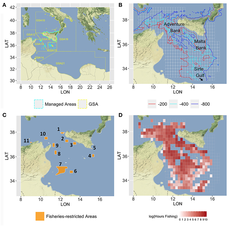
Figure 1. Map of the Strait of Sicily, in which (A) the GSAs 12–16, 19, and 21 are represented with the managed areas (in cyan dashed lines) where trawl fishing is forbidden; (B) the main bathymetries (−200, −400, and −800) are represented together with the 15 ×15 nautical miles grid (in gray) used to set up the model; (C) the network of the nine areas considered for the spatial scenarios are represented by orange polygons, numbered in a clockwise order: 1, Egadi islands; 2, East of Adventure Bank; 3, West of Gela Bank; 4, East of Malta Bank; 5, Capo Passero; 6, “Fondaletto”; 7, “Mammellone”; 8, West of Pantelleria; 9, Cape Bon shoal; 10, Skerki Bank; 11, Galite Bank; (D) the mean annual fishing effort, in the period 2012–2016, is represented with a red-scale color (log of total fishing hours). Figures were created using the R package ggmap (Kahle and Wickham, 2013) using Map tiles by Stamen Design, under CC BY 3.0 and data by OpenStreetMap contributors (2017).

The SoS is one of the largest areas of occurrence of demersal-shared stocks in the Mediterranean. These include the stocks of DPS and HKE shared by Italian, Tunisian, and Maltese fisheries. The DPS is the main target species of trawling amounting to about 50% of the total landings of the Italian fleet. European hake is the main commercial by-catch of trawlers targeting DPS, being about 10% of their total landings. Two other economically important species in the SoS are those of ARS and MUT. ARS is fished almost exclusively by the Italian trawlers on slope bottoms of the entire SoS and amounts to about 10% of the landing. According to Gargano et al. (2017), red mullet off the Southern coast of Sicily forms a stock unit that is exploited almost exclusively by Italian trawlers operating on shelf bottoms. Latest assessments carried out within the framework of the GFCM and supported by the MedSudMed FAO regional project revealed an overfishing status for all the stocks with the exception of the red mullet. To improve the exploitation of the stocks, a reduction of fishing mortality, especially on the juvenile fractions of the stock of DPS and HKE, was recommended (SAC, 2018). It should also be remembered that the SoS has been prioritized for conservation (de Juan et al., 2012; Oceana, 2012) with several sites, mainly offshore banks, and seamounts, identified for their future inclusion in a Mediterranean network of marine protected areas. Currently, different areas subject to trawling restrictions are already implemented in the SoS (Figure 1C). In the northern sector, these include the Egadi Marine Protected Area and three FRAs established in 2016 (FAO, 2016) in correspondence of the main stable nurseries of European hake and deepwater pink shrimp identified along the Italian–Maltese continental shelf. In the southern part of the SoS, the wide area called “Mammellone” subject to trawling restrictions has been implemented by an agreement between Italy and Tunisia with the aim of fish restocking. All these areas were considered as forming a network of spatial closures to be used in the simulation scenarios of SMART. Additionally, four further areas located in the Tunisian platform were considered. They are potential nurseries of European hake as preliminarily identified within the MANTIS project by integrating maps drawn by fishers (LEK) and a predictive model of hake recruits distribution developed in the south-central Mediterranean (Garofalo, 2018).

Data

The fleet of Italian trawlers operating in the SoS during the year 2016 accounted for 395 vessels with length-over-all (LOA) ≥ 12 m. A total of 367 of these are equipped with vessel monitoring systems (VMS) and were considered for this study. The LOA of each vessel was retained from the EU Community Fishing Fleet Register⁴ and used as the best proxy of vessel's fishing capacity (Russo et al., 2018). The fishing effort deployed by each Italian trawler operating in the SoS was quantified, for the 60 months in the years 2012–2016, using VMS data provided by the Italian Ministry of Agricultural, Food and Forestry Policies, within the scientific activities related to the Italian national program implementing the European Union Data Collection Framework in the Fishery Sector. VMS data were processed using the VMSbase platform (Russo et al., 2011a,b, 2014a, 2016), an R add-on package providing a complete suite of tools for cleaning, interpolating, and filtering of VMS pings. The amount of fishing effort (in fishing hours) was estimated for each trawler/month/cell of the grid (Figure 1D). Although logbook data could represent the main source of information about catch and landing (Gerritsen and Lordan, 2011), several reasons (see Russo et al., 2018 for a detailed list) supported the adoption, in Italy and other similar Mediterranean countries, of a statistical sampling scheme, based on questionnaires filled by researchers at harbors, to collect vessel-specific monthly landing data (EC, 2008; EUROSTAT, 2015). These data for the Italian trawlers operating within the SoS in the period of interest were therefore used in this study. Catch data by species were derived from the sampling for biological data from commercial fisheries (CAMPBIOL) carried out as part of the Italian plan for DCF. Sampling was performed monthly to evaluate the quarterly length distribution of species in the catches. Data were collected both by scientific observers onboard commercial bottom trawlers and by fishers through self-sampling. These data were used to obtain the age composition of CPUE. The geo-referenced data of abundance at sea of the four target species were collected during scientific bottom trawl surveys: the “Mediterranean international bottom trawl survey” (MEDITS) carried out in the northern part of the SoS from 1994 to 2016 and the Italian national trawl surveys GRUND (Relini, 2000) carried out in a large area covering GSA 16 and portions of adjacent GSAs from 1990 to 2008. The MEDITS data were used for both tuning the catch data and estimating the spatial distribution by age of each species, while the GRUND data were used only for estimating the spatial distribution by age class. The economic data were derived from the sampling for economic data from commercial fisheries as part of the Italian plan for DCF. The raw data are composed of 587 records of costs, for each vessel subject to the economic survey available for the 2-year period of 2014–2015 (301 vessels for 2014 and 286 for 2015). Each record is related to the activity of a single fishing unit and the sample is representative approximately of the 56% of the VMS monitored fleet. The cost data report the amount of expenses sustained by each vessel to perform the fishing operations disaggregated into three main categories of costs: spatial-based, effort-based, and production-based. The spatial-based costs summarize all the economic items proportional to the expenses linked to the spatial pattern; the effort-based costs gather all the fixed costs connected to the daily activity independently from the location choices (i.e., crew salary, maintenance, insurance); the production-based costs summarize the costs incurred by the commercialization of the landed species and it is proportional to the landed quantities.

Model Structure and Workflow

The spatial domain of the SMART model for the SoS was defined as a grid with 500 square cells (15 ×15 nautical miles) (Figure 1B). This grid is coherent with the one defined by the GFCM⁵ Although several studies demonstrated that large spatial scale could lead to distortions in the analysis of fishing effort and related spatial indicators (Mills et al., 2007; Lambert et al., 2012; Hinz et al., 2013), the spatial resolution applied in this study was selected to harmonize coverage (i.e., number of observation by cell) over different data sources (i.e., VMS, landings and CAMPBIOL) and to limit the number of spatial units (cells), which is a critical parameter affecting computational features of the model. The rationale of the model, as well as the workflow of the smartR package, can be summarized in the following logical steps:

1. Processing landings data, combined with VMS data, to estimate the spatial/temporal productivity of each cell, in terms of aggregated landings per unit of effort (LPUE) by species, according to the method described and applied in Russo et al. (2018);

2. Processing biological data to estimate LPUE by age and by species, for each cell/time;

3. Analyzing VMS data to assess the fishing effort by vessel/cell/time;

4. Combining LPUE by age with VMS data to model the landings by vessel/species/length class/time/cell;

5. Estimating the cost by vessel/time associated with a given effort pattern and the related revenues, as a function of the landings by vessel/species/length class/time (step 4);

6. Combining costs and revenues by vessel, at the yearly scale, to obtain the profit, which is the proxy of the vessel performance. profit could be aggregated at the fleet level to estimate the overall performance;

7. Using estimated landings by species/age, together with survey data, to run mice model for the selected case of study in order to obtain a biological evaluation of the fisheries.

Each of these steps corresponds to a different module of the R package. The relationship between each module of SMART (in gray) and its data sources (box at the center of the image) is represented in Figure 2A. The quantities (e.g., LPUE) generated by the different modules, and used in the intermediate steps of the model, are represented in dark yellow.

FIGURE 2

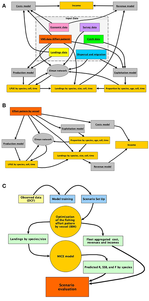
Figure 2. Representation of (A) the architecture of the smartR model, showing as the different input data are processed by different modules; (B) summary of the IBM implemented to obtain the economic quantities to be optimized in relation to the effort pattern of each vessel; (C) the typical workflow, from DCF data to the final MSE evaluation.

While the different modules are described in detail in the successive subsections, in Figure 2B, the rationale of the simulation approach applied at the level of the individual trawler is summarized. Figure 2B also represents the flux diagram for the sequence of steps in the previous bullets points. SMART includes an IBM predicting the allocation of the fishing effort for each vessel under different scenarios. Starting from the observed effort pattern by vessel, several scenarios can be virtually applied in order to predict the pattern resulting from the adaptation of each vessel to the new situation. Firstly, p_{c, t, v}, which is the spatial (for each cell c) and temporal (for each time t) distribution of the effort for each vessel v, is reconstructed using VMS data. Afterward, this distribution is modified in space and/or time according to the selected scenario. For instance (scenario with FRA), p_{c, t, v}, is set to zero if c ∈ FRA, where FRA is the set of cells closed to fisheries. Otherwise, p_{c, t, v} is set to zero if t ∈ B, where B is the set of times during which a temporal stop of fishing activity is set. Since it is possible to assume that the effort would simply reallocate according to the remaining distribution rescaled to the total effort, candidate configurations were obtained by multinomially sampling points when c ∉ FRA| t ∉ B from this distribution. Checking whether the associated profit is greater than the previous ones will validate this candidate configuration (Figure 2B). If the configuration is not valid, it will be discarded and another candidate configuration will be drawn. Otherwise, p_{c, t, v} is updated and the whole procedure is repeated until a convergence criterion is met. These steps are repeatedly carried out, for each vessel, in IBM optimization (Figure 2C). When the optimization ends for all the vessels in the fleet, aggregated revenues, costs, and profit can be computed for the whole fleet. In the same time, the total landings by species/age (or size) are passed to the MICE model devised to assess the biological consequences of the selected scenario. Finally, economic and biological outcomes for the selected scenarios are compared in a Management Scenario Evaluation (MSE). A complete list of input data and related features is provided in Table S1.

Spatial LPUE and Age Structure of Landings

Monthly landings were combined with VMS data (using the fishing vessel and temporal range of the fishing activity as references) to estimate the monthly LPUE for each species and cell of the grid (see Russo et al., 2018, for an extensive description of this procedure). The LPUE obtained are initially aggregated by species and across all the different age classes (cohorts). The aggregated LPUE were than transformed in LPUE by size using the biological data (CAMPBIOL) about length composition of catch. The age of each individual was estimated from its length to determine the demographic structure of catch and thus to convert the length–frequency distribution (LFD) of catch into an age–frequency distribution. The growth parameters, according to the Von Bertalanffy model, were estimated internally to the SMART model (see Table 1 for the estimated values). The Von Bertalanffy model is described by the differential equation:

$\begin{array}{ll}\frac{dL}{dt}=k_1(L_{\infty }-l)& (1)\end{array}$

where L is the length at time t, k₁ is the growth rate parameter, and L_∞ is the asymptotic length at which growth is zero. The commonly employed parametrization of the solution is:

$\begin{array}{ll}L(t)=L_{\infty }(1-e^{-k_1(t-t_1)})& (2)\end{array}$

where t₁ is the time at which an individual fish would have had zero length.

TABLE 1

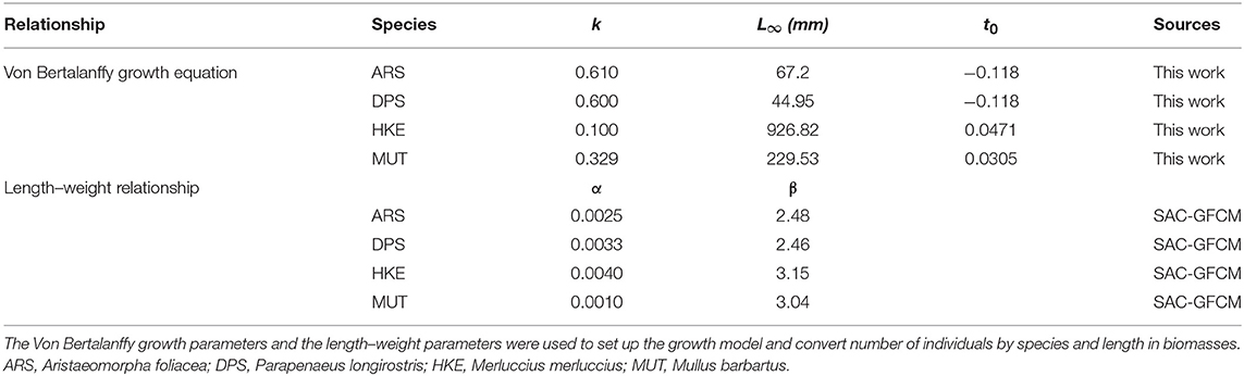
Table 1. Biological parameters not referred to age.

Providing the maximum supposed number of components (cohorts) of the mixture, the routine implemented in smartR returns:

1. The estimated age by individual and species;

2. A vector of cohorts proportion by species, time (month), and cell. these proportions are used to split the LPUE by species/month/cell into LPUE by species/age/month/cell, using the length–weight parameters in Table 1.

Sex of each individual was not considered and parameter values for the unsexed class were used. The mixture analysis implemented in R is based on the Markov Chain Monte Carlo (MCMC) stochastic simulation engine JAGS (Just Another Gibbs Sampler; Plummer, 2003). An extensive description of this procedure is in preparation.

Connectivity

smartR allows integrating the role of connectivity among the cells or set of cells, composing the spatial model. Two aspects of connectivity were considered: the connectivity due to larval dispersal from spawning to nursery areas and that concerning the reproductive migration from the nursery/feeding grounds to spawning areas. To do this, the original version of the Elman Multilayer Perceptron Network (EMPN) of SMART (Russo et al., 2014b) was modified to predict the LPUE by species/age of each cell i at time t using as input the following variables: (1) the amount of fishing effort at time t − 1; (2) the time of the system (in months); (3) the LPUE by species/age of cell i at time t − 1; and (4) the weighted mean LPUE by species/age at time t − 1 in the set of donor/receiving cells defined for each cell of the grid (Figure 3). The set of donor/receiving cells was defined using a connectivity matrix containing the estimated flux, by species/age, for each pair of cells. Fluxes were quantified as positive values for the donor cells and negative for the receiving cells. This connectivity matrix was generated, for the different life stages of each species, using the procedure described in the next subsections. The LPUE by species/age were computed disaggregating the LPUE by species described in the section Spatial LPUE and Age Structure of Landings with the proportion by age described in the same section. In this study, it was assumed that the grid defined above defines the boundaries of the system, for the four species. Hence, it was also assumed that immigration and emigration fluxes between the system and the adjacent areas are negligible.

FIGURE 3

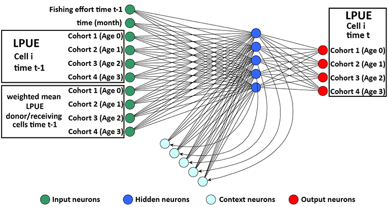
Figure 3. Representation of the Elman network devised to process temporal time series of LPUE for each species in the model. The input layer comprises three blocks of neurons: one for fishing effort and time, one for the temporal series of LPUE, by age, in cell I, and one for the temporal series, by age, of mean LPUE in the donor/receiving cells. The input neurons directly propagate the information to the basic hidden neurons. At each step of the training procedure, the updated pattern of the basic hidden neurons is memorized by the context neurons and, at the successive step, propagated to the basic hidden neurons together with the new information in the input neurons. The output layer contains as many neurons as the number of age classes of the species considered. Modified from Russo et al. (2014b).

Larval Dispersal From Spawning to Nursery Areas

The connectivity between spawning and nursery areas was investigated by the adoption of numerical modeling (Gargano et al., 2017). The model consists of an off-line larvae transport model that runs with stored ocean model hindcasts (North et al., 2006). The seeding of numerical particles varies with the dimension of the spawning area of each species, and it ranges in between 530 and 934 per day. Particles are passively advected by ocean currents; once they reach the appropriate age for settlement, the model tests the location of particles to determine if they are found inside or outside a nursery area. Advection equation is solved (using, a fourth-order Runge-Kutta scheme) for the current velocities at the particle location using an iterative process that incorporates velocities at previous and future times to provide the most robust estimate of the trajectory of particle motion in water bodies with complex fronts and eddy (Dippner, 2004). A random displacement model (Visser, 1997) is implemented within the larval transport model to simulate sub-grid scale turbulent particle motion in the vertical direction and a random walk model is used to simulate turbulent particle motion in the horizontal direction. The spatial information about the SoS domain that was used to implement the Lagrangian model includes the modeled hydrodynamic variables (i.e., zonal and meridional current velocity at all computed depths) and geographical location and shapes of spawning and nursery areas of the four target species (Colloca et al., 2013). Hydrodynamic variables with daily frequency were retrieved by the Copernicus⁶ Marine platform that is responsible for the dissemination of multiannual dataset of the Mediterranean Forecasting System (MFS). MFS reanalyses components are derived by the application of the ocean general circulation model NEMO-OPA (Madec, 2008) that is implemented in the Mediterranean basin at 1/16° by 1/16° (about 6 km) horizontal resolution and 72 unevenly spaced vertical levels (Oddo et al., 2009). Geographical distributions of spawning and recruitment areas were available by observational datasets (Colloca et al., 2013); if not available, they were inferred by integrating substrate and bathymetry information, at a scale of 1:100,000 (EMODnet portal⁷, which are typical of juvenile recruits and adults of the target species.

The Lagrangian model uses external time step corresponding to the daily frequency of the released physics products of the zonal and meridional current velocities and an internal time step of 1,800 s, for stability reasons. Turbulent horizontal and vertical components are given by the constant value of 4.9 m² s⁻¹ in agreement with a numeric approach based on the computational grid spatial resolution (Okubo, 1971). During each model simulation, a numerical particle is released at the center of each grid cell (2.6 by 3.3 km) with daily frequency, within the edges of the spawning areas and with random depth along the water column. Since we do not model growth explicitly, in the absence of a defined relationship linking temperature and larval phase duration, larvae are assumed to reach the minimum length for settling in two time windows: 10–30 and 40–60 days after spawning. The 10–30 days group can mimic a fast-growing larvae being spawned during summer months, while the 40–60 days group can mimic larvae being spawned during winter months. For this reason, each model simulation includes two different values for the age of settlement and death of numerical particles.

The Lagrangian model runs for the period in between 2012 and 2015 for each target species, and the obtained results were processed to evaluate the origin of numerical particles that settle into defined nursery areas, hence providing connectivity information. At this intent, the particle fluxes (PFs) were computed with Equation 3. C_A is the number of numerical particles that settle in a nursery area (A) during the time range of the simulations (j). C_A is normalized by the number of particles (N_s) that are released in the spawning region.

$\begin{array}{ll}P{F}_s=\frac{1}{N_S}{\displaystyle \sum _{j=1}^n}{C}_{Aj}& (3)\end{array}$

Results are organized in connectivity matrices showing for each year and for each time windows the identification numbers of spawning and nursery areas and the ratio between released and recruited particles, representing the success of recruitment of the released particles. For DPS species, the Supplementary Materials report a graphical example of connectivity (Figure S1) using PFs (Equation 3), between known spawning and recruitment areas of the SoS.

Juveniles' Migration From Nursery/Feeding Grounds to Spawning Areas

The juveniles' migration patterns were investigated for each fish species following an empirical approach. Fish movements were derived by comparing the distribution in space of different age groups at different moments. In order to have complete coverage of the SoS, abundances by species and age were derived by integrating MEDITS dataset with GRUND survey and catch data. The merging procedure was carried out over a common sampling grid and consisted in the sum of the normalized abundances of the individuals from each dataset to obtain a single homogeneous distribution for each age class and fish species.

Although the two datasets slightly differ from each other, with MEDITS and GRUND campaigns occurring during summer and autumn months, respectively, this simplified merging procedure could be applied, with the investigated process being characterized by annual time scale. Furthermore, the use of normalized quantities allowed us to consider data from different sources and to focus the analysis on the relative distribution of the abundances of each age class. According to the species, the abundances by age were grouped distinguishing juveniles from adults, assuming these as individuals belonging to fully mature age groups (Table 2). The obtained datasets were adopted to infer the moving of fishes across age classes. Considering the abundance like a tracer, the transport equation for a conservative tracer was evaluated between age class groups (0 and higher). Potential migration from nurseries/feeding grounds to spawning areas for each species was hence computed inverting the conservation equation expressed by:

$\begin{array}{ll}\frac{dA}{\partial t}=\nabla F=-\frac{\partial U}{\partial x}-\frac{\partial V}{\partial x}& (4)\end{array}$

where A is the abundance, considered as a conservative tracer, and F is a flux that is, in turn, derived by the computation of the spatial gradient between abundances of adjacent age classes.

TABLE 2

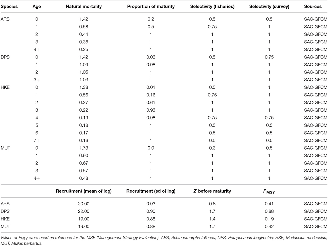
Table 2. Biological parameters referred to age, used to set up MICE model.

For each fish species, the abundance distributions of each age class were considered a sequence of steady states. Within this context, Equation 4 was treated following a numerical approach obtaining the following algebraic expression for the horizontal components of F:

$\begin{array}{ll}{U}_{x,y}=\left(A_{x+1,y}^{t+1}-A_{x,y}^t\right)+\left(A_{x-1,y}^{t+1}-A_{x,y}^t\right)& (5)\end{array}$

$\begin{array}{ll}{V}_{x,y}=\left(A_{x,y+1}^{t+1}-A_{x,y}^t\right)+\left(A_{x,y-1}^{t+1}-A_{x,y}^t\right)& (6)\end{array}$

where U_{x, y}, V_{x, y} represent the horizontal components of F for the point x, y of the regular mesh previously described, $A_{x,y}^t$ is the number of individuals of age class t at point x, y, the subscript indicates a shift forward or backward in the mesh point of 1 unit, in the meridional or zonal directions, and the superscript +1 indicates a shift forward in the age class. Therefore, for each point of the regular sampling grid, the total number of individuals migrated to the nearest points between adjacent ages classes were estimated.

This method assumes that the potential migration among subsequent age classes is based on cell length. Thus, the obtained results only provide qualitative information on the direction pattern between age classes. As an example, in the Figure S2, the migration patterns obtained considering as input data for Equations 4 and 5 the juvenile and adult stages distributions of the DPS are depicted.

Economic Models for Costs and Revenues

The economic performance of the fleet results from the balance between costs and revenues of all the vessels actively involved in the fishery. Thus, to evaluate the economic performance of the fishing fleet, it is firstly necessary to model, at the scale of the single vessel, the operational cost linked to the fishing activity with the corresponding revenue and then to aggregate revenues and costs for the whole fleet. For each fishing vessel, the economic performance is determined by the profit resulting from its strategy, which results from the subtraction of the costs from the revenues. Here, the strategy is represented by the fishing grounds selection and the amount of effort deployed. Two blocks of economic parameters were considered to estimate costs and revenues related to the fishing activity of each trawler. Namely, costs were modeled in terms of their “spatial-based,” “effort-based,” and “production-based” components. Spatial-based costs are a function of spatial locations of fishing operations (i.e., the fishing grounds). Given that, for each vessel, different fishing grounds are characterized by different distances from the harbor of departure (computed as the linear distance between the center of each cell and the positions of the harbors), these costs are mainly related to the fuel consumption. Monthly values of fuel price were provided by the Italian National Institute of Statistics (ISTAT⁸

Accordingly, a spatial index (SI) was computed, for each vessel v and time t (month) as:

$\begin{array}{ll}S{I}_{v,t}={\displaystyle \sum _{c=1}^C}{d}_{v,c}{E}_{c,v,t}& (7)\end{array}$

where d_{v, c} is the distance between cell c and the harbor of departure for the vessel v, and E_{c, v, t} is the amount of effort (in hours of fishing) deployed by vessel v in the cell c during the time period t.

The relationship for spatial-based costs (SC), is then defined as:

$\begin{array}{ll}S{C}_{v,t}={\alpha \times LO{A}_v\times SI}_{v,t}& (8)\end{array}$

where SC_{v, t} are the spatial-based costs, in Euros, bore by vessel v during the time period t, SI_{v, t} is the spatial index defined above, LOA_v is the length-over-all of the vessel v, and α is the parameter to be estimated. According to Lindebo (2000) and the authors' experience, de-rating practices and the exclusion of auxiliary engines could lead to relevant differences between official Engine Power (KW) and maximum effective KW. Moreover, official records for EKW have proved to be completely skewed, suggesting the adoption of alternative parameters (Sardá, 2000). Thus, LOA was preferred to KW because we consider the official data about LOA more reliable than those about KW. While a detailed reconstruction (e.g., at the scale of single trip) of the fuel consumption is beyond the scope of this paper, the spatial-index we computed includes both the amount of effective time fishing by cell/vessel and the relative distance by cell. In this way, our target is an aggregated estimation of fuel cost (SC_{v, t}), mainly driven by the vessel-specific fishing footprint (SI_{v, t}).

The effort-based costs are independent of the locations of fishing operations and are defined as a function of the number of days at sea spent by each vessel. This component of the costs is devised to consider the labor costs (e.g., salaries) and the other expenses (repair/maintenance of the vessel) directly linked to the temporal duration of fishing activities. VMS data allow us to easily assess the number of days at sea (DS) for each vessel v during the period t. Thus,

$\begin{array}{ll}E{C}_{v,t}={\gamma \times LO{A}_v\times DS}_{v,t}& (9)\end{array}$

where EC_{v, t} are the effort-based costs, in Euros, bore by vessel v during the time period t and γ is the parameter to be estimated. Here, the term LOA_v is aimed at capturing the effect of vessel size in terms of, for instance, the crew size.

The production-based costs are linked to the amount of landings (e.g., commercialization costs). They are defined as:

$\begin{array}{ll}P{C}_{v,t}={\mu \times LV}_{v,t}& (10)\end{array}$

where PC_{v, t} are the production-based costs, in Euros, beard by vessel v during the time period t, μ is the parameter to be estimated, and LV_{v, t} are the landing value, which is the product of landings by species and size times the respective prices.

The total costs (TC) for vessel v during the period t are:

$\begin{array}{ll}T{C}_{v,t}=S{C}_{v,t}+E{C}_{v,t}+P{C}_{v,t}+\epsilon & (11)\end{array}$

The corresponding Revenues (R) for vessel v during the period t are:

$\begin{array}{ll}{R}_{v,t}={\displaystyle \sum _{s=1}^S}{\displaystyle \sum _l^L}{q}_{s,l,t}\times p_{s,l,t}& (12)\end{array}$

where q_{s, l, t} is the amount of landings for the species s and size class l during the period t by the respective price at the market (p_{s, l, t}).

Thus, the Profit (P) for vessel v during the period t is:

$\begin{array}{ll}{P}_{v,t}=R_{v,t}-T{C}_{v,t}& (13)\end{array}$

And, for the whole fleet, during the year y:

$\begin{array}{ll}{P}_y={\displaystyle \sum _{t=1}^T}{\displaystyle \sum _{v=1}^V}{P}_{v,t}& (14)\end{array}$

Values of prices at the market by species and length class, together with the price of fuel, were partially retrieved by Russo et al. (2014b) and integrated using the public database provided by the “Istituto di servizi per il mercato agricolo alimentare” (ISMEA⁹).

MICE Model

The new version of SMART adopted a MICE approach to model the population dynamics of the exploited resources (Morello et al., 2014; Plagányi, 2014; Punt et al., 2016). The model describes the exploitation of resources by fisheries as well as the main inter-specific and intra-specific trophic interactions (Figure 4). Unlike HKE and DPS, MUT, and ARS were considered as stand-alone stocks not characterized by a trophic relationship with other investigated species. The chosen framework models a simple Statistical Catch at Age (SCAA) with a basic population dynamic where the catch-at-age datasets are fitted for multiple cohorts simultaneously and the fishing mortality is split into age and year components (Doubleday, 1976) where the catch-at-age datasets are fitted for multiple cohorts simultaneously and the fishing mortality is split into age and year components. The age-structured population dynamic is designed with a forward projection method, and it is modeled as:

$\begin{array}{ll}{\text{N}}_{\text{ya}}=\{\begin{array}{c}{\text{R}}_0{\text{e}}^{ϵ\text{y}}\\ {\text{N}}_{\text{y}-1\text{a}-1}{\text{e}}^{-{\text{Z}}_{\text{y}-1\text{a}-1}}\\ {\text{N}}_{\text{y}-1\text{x}-1}{\text{e}}^{-{\text{Z}}_{\text{y}-1\text{x}-1}}+{\text{N}}_{\text{y}-1\text{z}}{\text{e}}^{-{\text{Z}}_{\text{y}-1}}\end{array}& (15)\end{array}$

where N_ya is the number of individual of age a in the year y, R₀ is the median recruitment with a yearly deviation of e^ϵy, and x is the maximum age class. Only one source of uncertainty was considered, namely, process error, due to variation in future recruitment. To do this, 100 projections of the model were carried out and, in each projection, the future recruitment is generated as:

$\begin{array}{ll}{N}_{y,0}^s=R_0^s{e}^{{\epsilon }_y^s-{({\sigma }_R^s)}^2/2}where{\epsilon }_y^s~N(0;{({\sigma }_R^s)}^2)& (16)\end{array}$

where $N_{y,0}^s$ is the number of age-0 animals of species s at the start of year y, $R_0^s$ is the average number of age-0 animals of species s, and ${\sigma }_R^s$ is the extent of variation in recruitment for species s.

FIGURE 4

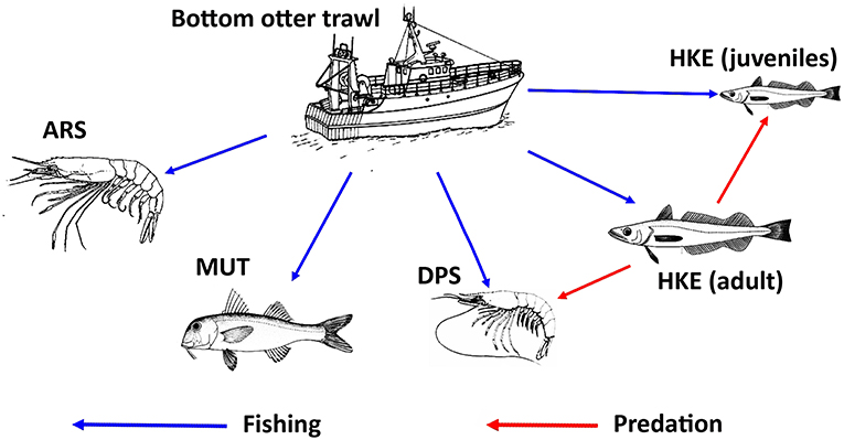
Figure 4. Representation of the relationships between trawl fishing and the main stocks exploited in the Strait of Sicily, together with the main trophic relationships between stocks. Adult HKE is a predator of DPS and HKE juveniles. MUT and ARS were considered as stand-alone stocks with no trophic relationship with other investigated species. The source of the image for ARS is Fischer et al. (1987). The source of the images for DPS, HKE, and MUT is FAO (2017). All these images were reproduced with permission of FAO Copyrigh Office.

In general, the total mortality Z of the age group during year y is defined as:

$\begin{array}{ll}{Z}_{ya}=M_a+S_a{F}_y& (17)\end{array}$

where M_a is the natural mortality rate at age a, S_a is the fishery selectivity at age a, and F_y is the fishing mortality of the year y. The prey–predator interactions are modeled as a secondary source of mortality. For DPS, this relationship was modified to account the predation by HKE (Carrozzi et al., 2019):

$\begin{array}{ll}{Z}_{ya}=M_a^{1,DPS}+S_a{F}_y+M_{y,a}^{2,DPS}& (18)\end{array}$

where $M_a^{1,DPS}$ is the natural mortality rate at age a, S_a is the fishery selectivity at age a, F_y is the fishing mortality of the year y, and $M_{y,a}^{2,DPS}$ is the rate of natural mortality during year i for DPS of age a due to HKE predation, while for HKE, the total mortality was modified to account for the cannibalism behavior of older HKE that predates younger HKE with age smaller than or equal to 2 years (Carrozzi et al., 2019), giving:

$\begin{array}{ll}{Z}_{ya}=M_a^{1,HKE}+S_a{F}_y+M_{y,a}^{2,HKE}& (19)\end{array}$

The mortality rate for DPS and HKE of age ≤ 2 can be modeled according to:

$\begin{array}{l}{M}_{y,a}^{2,DPS}={\tilde{M}}_a^{DPS}\left(\frac{{\alpha }^{DPS}{B}_y^{HKE}}{{\beta }^{DPS}+B_y^{DPS}}-1\right)\\ M_{y,Age\le 2}^{2,HKE}={\tilde{M}}_{Age\le 2}^{HKE}\left(\frac{{\alpha }^{HKE}{B}_{y,Age>2}^{HKE}}{{\beta }^{HKE}+B_{y,Age>2}^{HKE}}-1\right)& (20)\end{array}$

Additionally, the population dynamic of HKE is also defined in terms of survivability due to abundances of preys:

$\begin{array}{ll}{\tilde{S}}_{y,Age\le 2}^{2,HKE}=e^{{-M}_{y,Age\le 2}^{2,HKE}}& (21)\end{array}$

And the survival rate for HKE is modeled as:

$\begin{array}{ll}{\tilde{S}}_{y,a}^{HKE}=\frac{{\alpha }^{HKE}(B_y^{DPS}+B_{y,Age\le 2}^{HKE})}{{\beta }^{HKE}+(B_y^{DPS}+B_{y,Age\le 2}^{HKE})}& (22)\end{array}$

The parameterization of the secondary mortality M², for both DPS and HKE^{Age ≤ 2}, and the survivability of ${\tilde{S}}_{y,a}^{HKE}$ are constrained by α^s and β^s as the parameters of the interaction functions, ${\tilde{M}}_a^s$ is a measure of mortality, and $B_{y,a}^s$ is the start-year biomass for species s, where α = β + 1 and, for the predator (HKE older than 2 years):

$\begin{array}{ll}\beta =\frac{1-\chi }{2{}^{*}\chi -1}& (23)\end{array}$

While for the prey (DPS and HKE younger than 2 years):

$\begin{array}{ll}\beta =\frac{2{}^{*}\chi -1}{1-\chi }& (24)\end{array}$

To ease the input parameterization, we replaced biomass by relative biomass:

$\begin{array}{ll}{P}_y^{Preys}=\frac{B_y^{DPS}+B_{y,Age\le 2}^{HKE}}{B_0^{DPS}+B_{0,Age\le 2}^{HKE}}& (25)\end{array}$

The parameters of Equation 20, ${\tilde{M}}_a^{DPS}$, α^DPS, and β^DPS for DPS and ${\tilde{M}}_{Age\le 2}^{HKE}$, α^HKE, and β^HKE for HKE of age ≤ 2, are then specified by defining the parameters χ^DPS and χ^HKE as the survival coefficients and Ω^DPS and Ω^{HKE ≤ 2} as the predation coefficients, i.e.,

$\begin{array}{ll}{\Omega }^{DPS}{M}_a^{DPS}=M_{y,a}^{2,DPS}{\Omega }^{HKE\le 2}{M}_a^{HKE}=M_{y,Age\le 2}^{2,HKE}& (26)\end{array}$

Values for χ and Ω are reported in Table 3. Furthermore, the catch at age in numbers for each year C_ya are estimated as:

$\begin{array}{ll}{C}_{ya}=\frac{S_a{F}_y}{Z_{ya}}{N}_{ya}(1-e^{{-Z}_{ya}})& (27)\end{array}$

While the catch-in-weight for year y is:

$\begin{array}{ll}\widetilde{C_y}={\displaystyle \sum _a}{w}_{a+1/2}{C}_{y,a}& (28)\end{array}$

where w_a is the weight of animal of age a. The catch-at-age datasets are assumed to be multinomially distributed, while the survey estimates of abundance by age class are assumed to be log-normally distributed with a standard error of the log that is independent of age and year.

TABLE 3

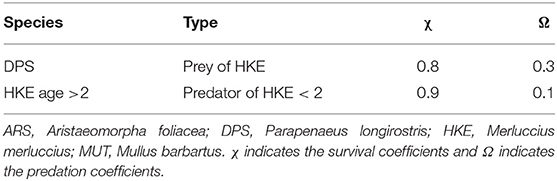
Table 3. Parameters of the trophic relationships considered into the MICE model.

The spawning biomass, for each species and year, is accounted for in the middle of the year as modeled by the expression:

$\begin{array}{ll}SS{B}_y={\displaystyle \sum _{a=0}^x}{w}_a{m}_a{N}_{ya}{e}^{-0.5Z_{ya}}& (29)\end{array}$

The model time period runs from 2012 to 2016.

Model Validation

The trained smartR model was checked, for the years 2012 to 2016, by comparing the modeled SSB and total annual landings, by species, with the official DCF ones. The outputs of this comparison are reported in the Figure S3.

Simulated Scenarios

The list of management scenarios explored is summarized in Table 4. The first one was represented by the status quo providing a baseline for assessing the potential effect of the other scenarios. The Effort Regime scenario was based on the Multi-Annual Management Plan adopted by the Italian Governments and by the EC for demersal fisheries in the SoS. Moreover, two sets of scenarios were used to evaluate the effectiveness of spatial and temporal closures of trawling, respectively. Spatial closures corresponded to (1) the year-round closure of trawl fishing in the three FRA identified by the REC.CM-GFCM/40/2016/4 of GFCM; (2) the year-round closure of the full network of FRA (Figure 1C) identified within the MANTIS project, which comprises the three GFCM FRA off the Sicilian coast and other nurseries of hake identified with the support of the fishers' LEK off the African coast. Temporal closures corresponded to two scenarios suggested by stakeholders (fishers) within a series of participatory meetings organized by the MANTIS project and held in 2018 in Mazara del Vallo and Portopalo di Capo Passero, two of the main Sicilian harbors hosting trawlers: (1) the so-called “Winter stop,” which is the complete stop of trawl fishing in February and March, followed by 2 months of reduced activity (3 fishing days per week instead of 5 as happens in the rest of the year); (2) the so-called “Summer stop,” which is the complete stop of trawl fishing in September and October, followed by 2 months of reduced activity (3 fishing days per week instead of 5 as happens in the rest of the year).

TABLE 4

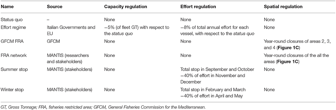
Table 4. Summary of the different scenarios compared through a simulation approach.

For each scenario, a series of 100 simulations were carried out by (1) using the years 2012–2016 to set up and train the model on observed data; (2) simulating the entry into force of management action in 2017; (3) estimating the displacement of the fishing effort and the related landings, costs, revenues, and profit; (4) estimating the new exploitation pattern (F at age for each species) and using it to run the MICE model and projecting its effects on stocks along a 5-year period in terms of Spawning Stock Biomass of each stock.

An MSE was carried out by comparing the overexploitation rate (defined, for each stock, as the ratio between the estimated F and the most recent value of F_0.1, as proxy of F_MSY, available in the literature), the ratio between the mean SSB forecast for the years 2018–2022, the mean SSB for the years 2012–2016, and the forecast profit for the fleet. Thus, nine parameters (four values of $\frac{F}{F_{0.1}}$, four values of $\frac{{SSB}_{2017-2022}^{Scenario}}{{SSB}_{2017-2022}^{Statusquo}}$, and one value for profit) were compared across the different scenarios.

Results

Spatial LPUE and Age Structure of Landings

Given that a detailed analysis of LPUE in space and time is beyond the scope of this paper, the description was limited to the mean pattern by species (Figure 5). The estimated LPUE for the four species were characterized by different ranges. The highest mean values were associated to DPS, reaching 2 kg per meter of LOA and hour of fishing, followed by ARS (0.7 kg/m/h), HKE (0.6 kg/m/h), and MUT (0.3 kg/m/h). The main fishing grounds of ARS were distributed offshore in the central region of SoS, west of Maltase islands, and in the southern-east corner of the area. Main fishing grounds for DPS along the northern sector of the SoS were distributed in separated areas including the northwest corner of the Sicily, a large area out of Marsala, and the eastern border of the Malta Bank. On the contrary, the DPS fishing grounds off the African coasts were distributed seamlessly between 100 and 400 m depth. This spatial pattern is very similar to the one of HKE, the main commercial bycatch of DPS trawling. Finally, the fishing grounds of MUT were concentrated in three main areas: the whole Adventure bank, the east side of Sicily, and a large area off the Tunisian shelf. Figure 6 represents, for each species, the mean proportion of catch by age/cell. These closely follow the corresponding patterns of mean LPUE by species (Figure 5). It is worth noting that (1) for ARS, the different age classes were consistently overlapped in the three fishing grounds; (2) DPS showed a progressive shift of the spatial distribution, according to the age, toward deeper areas; (3) HKE cohorts occupied the same fishing grounds of DPS, but with different proportion according to age; (4) given the lack of information on the coastal areas off Tunisia and Libya, the first cohort of MUT seems to be present only near the Sicilian coast, whereas older age classes are progressively concentrated in the offshore margin of the Adventure Bank and Tunisian coast.

FIGURE 5

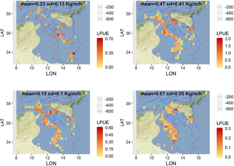
Figure 5. Spatial distribution of LPUE (kg/m/h) by species, as the annual mean for the period 2012–2016. Figures were created using the R package ggmap (Kahle and Wickham, 2013) using Map tiles by Stamen Design, under CC BY 3.0 and data by OpenStreetMap contributors (2017).

FIGURE 6

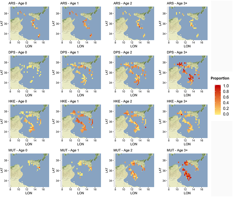
Figure 6. Distribution of the main different age classes, by species, in terms of proportion of landings. Age classes older than 3 years were aggregated to reduce the number of submaps. Figures were created using the R package ggmap (Kahle and Wickham, 2013) using Map tiles by Stamen Design, under CC BY 3.0 and data by OpenStreetMap contributors (2017).

According to the different measures corresponding to each scenario of Table 4, SMART returned estimates of the expected fishing effort pattern by vessel, and then at the aggregated level of the fleet, including the fishing effort displacement, if any, under different management scenarios (Figure 7). The Effort Regime scenario is likely to determine the abandonment of far fishing grounds, especially those located in the southeast part of the SoS and off Tunisia coasts. The establishment of the network of three FRAs defined by the GFCM is associated to a remarkable increase of the fishing effort around these, and a general increase in the south and southeast region of the SoS. This effort displacement and “border-effect” is even more evident in the FRA Network scenario, in which a kind of “ring” encloses the areas in the network. This scenario also highlights that a remarkable amount of the original effort is forced to be displaced out of the FRAs located near the Tunisian coasts. The temporal scenario represented by the “Summer stop” is associated to a substantial decrease in fishing effort on both the Sicilian and African shelves. In contrast, the “Winter stop” is likely to determine a decrease in effort on the more offshore and deeper grounds, including the slope.

FIGURE 7

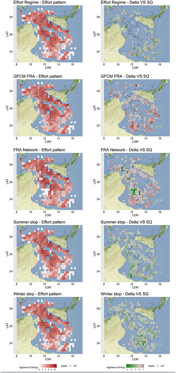
Figure 7. Optimized (mean over 100 simulations) fishing effort pattern, represented in red scale of Log Hours Fishing, and corresponding for the difference (Delta) with respect to the status quo (SQ), represented in green-red scale of Log Fishing Hours, for each scenario. The FRAs are represented as white polygon in the Spatial-based scenarios. These patterns represent the total yearly fishing effort for the Italian trawlers operating in the SoS. Figures were created using the R package ggmap (Kahle and Wickham, 2013) using Map tiles by Stamen Design, under CC BY 3.0 and data by OpenStreetMap contributors (2017).

The new fishing effort patterns from the different scenarios were associated to the pattern of fishing mortality by age and as $\overline{F}$ by species of Figure 8. The effect for the four species widely varies between scenarios. In general, the Effort Regime scenario determines a flat-cut of the fishing mortality, irrespectively of age. The spatial scenarios are associated to an increase of fishing mortality for ARS, and in particular for the FRA Network scenario. In contrast, these two scenarios are associated to a similar and clear reduction of fishing mortality for DPS and, in a much less remarkable way, for HKE. In the case of MUT, both spatial scenarios correspond to a reduction of fishing mortality, and especially the FRA Network scenario. On the other hand, temporal scenarios are linked to very different patterns of F at age. The Summer stop is always associated to a strong reduction of F_AAA, whereas the effects of the Winter stop are less detectable, although present. The variation of $\overline{F}$, expressed as % of the status quo, under the different scenarios is summarized in Table S2. Here, it is possible to observe that the largest reduction in fishing mortalities occurs for the Summer stop scenario, followed by the FRA Network and the GFCM FRA scenarios. The Effort Regime scenario corresponds to a strong benefit for HKE, but less for the other species.

FIGURE 8

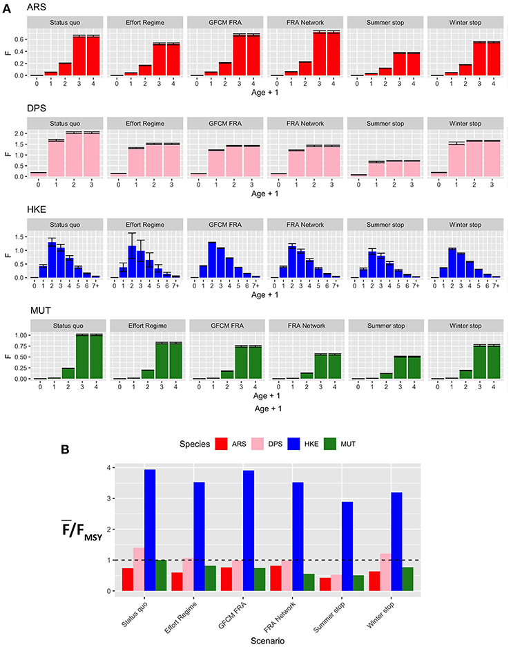
Figure 8. Barplot (mean and MSE) representing (A) F at age for each species and scenario, corresponding to the new fishing effort pattern after the introduction of a different management measure; (B) the corresponding overexploitation rate ($\frac{\text{F}}{{\text{F}}_{\text{MSY}}}$) for the different species and scenarios. Age ranges for the computation of Fw̄ere as follows: 1–3 years (ARS), 0–2 years (DPS), 1–5 years (HKE), and 1–3 years (MUT).

From an economic point of view, the performances of the different scenarios are summarized in Figure 9. The revenues related to landings of ARS, DPS, and MUT largely vary between the different scenarios, while those for HKE are quite similar, but always lower than those of the status quo. Summer stop and FRA Network are the two scenarios providing the lowest revenues for MUT. Costs by effort (as the number of fishing days) are lower for the temporal stops and the Effort Regime, while they are very similar in the status quo and the scenarios based on spatial closures. The pattern is similar for spatial costs (i.e., fuel), given that also this kind of cost is related to the number of fishing days. At an aggregated level, it is worth noting that profit is more or less equivalent under the different scenarios: always lower than in the status quo, with the highest values occurring for the GFCM FRA scenario and the other scenarios scoring similar values, around 70% of the status quo.

FIGURE 9

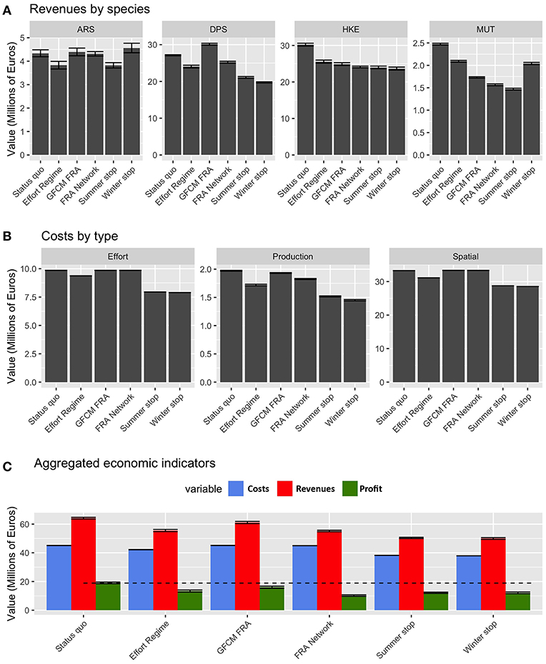
Figure 9. Barplot (mean and MSE) representing (A) the values of landings for each species and scenario, corresponding to the new fishing effort pattern after the introduction of the different management measures; (B) the corresponding costs by type and scenarios; (C) the aggregated costs, revenues, and corresponding profit by scenario, for the whole fleet of Italian trawler.

The estimated effects of the different scenarios on the SSB mid-term trends are represented in Figure 10. The variation of SSB 2017–2022 in the different scenarios as % of that of status quo is summarized in Table S3. In this case, the status quo represents a reference, and it is characterized by an increasing trend for ARS, a decreasing trend for DPS (rather sharp) and HKE, and a stable trend for MUT. The Effort Regime scenario is associated to positive effects on ARS and a clear decreasing trend for DPS, whereas MUT and HKE seem to be unaffected by this measure. The spatial scenarios (GFCM FRA and FRA Network) are instead characterized by positive effects on all the four species, which show increasing trends (ARS and MUT), or stable trends (DPS and HKE). The FRA Network scenario seems particularly effective for MUT. However, the best results are associated with the Summer stop scenario, in which all four species are expected to increase their SSB to levels twice as high as the status quo. In contrast, the Winter stop scenario does not show visible effects and the trends for the four species are very similar to those of the status quo.

FIGURE 10

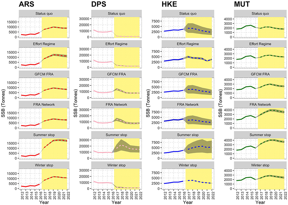
Figure 10. Reconstructed and predicted trends of Spawning Stock Biomass (SSB) by scenario for the different species. The white background identifies the observed time series (years 2012–2016), while the yellow background corresponds to prediction (years 2017–2022). In the predictions, the dashed line marks the mean trend over 100 simulations, while the gray area corresponds to the standard confidence interval.

Discussion

The application of SMART to the case study of trawl fishing in the SoS allowed exploring the possible consequences of six management scenarios in terms of variation from the status quo. The results, summarized in Figure 11, indicate that all alternative management scenarios are always associated, at least in the year of entry into force, to a decrease of the profit for the fleet with respect to the status quo, while the biological consequences on the stocks vary. In particular, the different options of FRAs closure are likely to allow reaching the sustainability targets in terms of fishing mortality for three of the four stocks considered, whereas the effect of the two temporal-based scenarios performed differently. After the status quo, the Winter stop scenario shows the worst performance among all the simulated scenarios in terms of recovery rate for SSB. Conversely, the Summer stop scenario gives the best biological effects, since it provides a mean SSB recovery rate larger than two for the stocks (Figure 11). However, this scenario corresponds also to a relevant reduction (around−40%) of the profit for the fleet, while the loss of gains is very reduced (about −10%) with the Winter stop. The situation is, from an economic point of view, even worse for the FRA Network. Thus, it seems that, overall, the GFCM FRA scenario seems to be the best spatial-based approach.

FIGURE 11

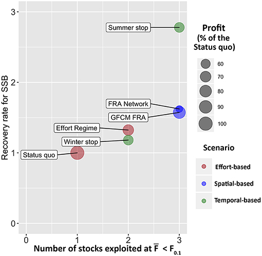
Figure 11. Management Strategy Evaluation of the different scenarios. The x axis corresponds to the number of stocks that are expected to be exploited at F_0.1 after the implementation of the corresponding scenario, the y axis corresponds to the mean recovery rate for SSB of the four stocks, computed as $\frac{{\text{SSB}}_{2017-2022}^{\text{Scenario}}}{{\text{SSB}}_{2017-2022}^{\text{Status quo}}}$. The size of the bubble represents the percentage of profit with respect to the status quo, for each scenario, in the first year (2017) of application. The color of the bubble groups the scenarios by type.

The consequences in terms of fishing effort displacement are also very different between scenarios. When spatial restrictions are applied (i.e., in GFCM FRA and FRA Network scenarios), effort is re-allocated in unclosed areas (Ba et al., 2019). Indeed, fishing effort is expected to increase around the edges of FRAs, as well as in already exploited fishing grounds. This “fishing-in-the-line” effect has been previously documented in the literature (Wilcos and Pomeroy, 2003; Horta e Costa et al., 2013; Cabral et al., 2017) and it is easily explainable by the fact that FRAs are likely to host higher biomasses and support spillover of resource for the fisheries. This chain of effects also suggests that, in the FRA Network scenario, the establishment of the new FRAs off the Tunisian coast could push the fleet farther (i.e., toward the fishing grounds near the coast of Libya) with larger costs for the fuel (Figure 9). Costs are always higher in spatial-based scenarios, even because the spatial component of cost is expected to exceed the value observed for the status quo. It is therefore coherent to observe that, for effort-based and temporal-based scenarios, the predicted fishing effort patterns are more or less a puzzle of areas in which the effort is expected to decrease (Figure 7).

Under the Effort Regime, the cells at the borders of the SoS (with the exception of those near the Sicilian coast) resulted abandoned, probably due to the cost to reach these fishing grounds. For Winter and Summer stop scenarios, the areas where the fishing effort decrease are much wider and only partially overlapping. The main differences are that under the Summer stop, the shallow bottoms off the Tunisian coast are less exploited, while during the Winter stop, the main reduction occurs on the slope off the Tunisian and the Libyan coast. In other words, the Summer stop is expected to reduce fishing effort in shallow grounds, while the Winter stop would determine an effort reduction in deeper areas. Considering both the effect of F and SSB, the Summer stop scenario showed a better performance than the Winter stop. Furthermore, the Winter stop seems to score similar to the Effort Regime: both scenarios support some improvements for HKE, but not enough to promote a switch of the system toward a sustainable level (Figure 10).

Analyzing the results by species, it seems that ARS has its own story, since this stock is the only one showing a sustainable fishing and an increasing trend in SSB for all scenarios, and in particular for the Summer stop. The pattern is similar for MUT, but this species is very close to F_0.1 in the status quo and only three different scenarios (GFCM FRA, FRA Network, and Summer stop) seem able to strongly improve the SSB for this species. DPS and HKE are the most challenging stocks since the overall performance of the different scenarios is closely dependent on the effects on these stocks. For both species, spatial-based approaches support in the mid-term the current levels of SSB, but only the Summer stop provides an improvement in the longer term (2022). One of the possible explanations is that these two species are linked by trophic relationships in the present modeling approach. This implies that fluctuations of the biomasses of DPS and HKE are not considered a “stand-alone,” as in single-species assessments, but non-synchronous trends are likely to occur as the time series expands. This could be observed in the Summer stop forecast for DPS and HKE, where local maxima are followed by a decrease in SSB.

In the new version of SMART, the fishing effort pattern of each vessel is modeled as the best configuration to maximizing individual profit. An emblematic case study on reallocation of fishing effort after the introduction of a large fisheries spatial closure was documented for trawl fishing in the Western Baltic Sea, where fishers redistributed effort to areas that have had relatively high LPUE to compensate for lost landings (Miethe et al., 2014). Within the optimization module of SMART, each vessel is considered as an individual agent that reacts to the different management measures by adapting its spatial configuration of effort to maintain the profit, at a monthly temporal scale, at the maximum level (as the difference between costs and revenues). In this way, the rationale of SMART is consistent with other spatial models (Mahévas and Pelletier, 2004; Bastardie et al., 2014; Miethe et al., 2014; Bartelings et al., 2015; Girardin et al., 2015; Mormede et al., 2017) designed to simulate how fishing effort could be re-allocated following any spatial or temporal closure of fishing grounds (Girardin et al., 2015). In fact the “implementation error,” which often impairs the effectiveness of management policies (Wilen, 1979), occurs exactly when fishermen behavior is not considered (Hilborn, 1985).

When comparing the two “scaled” spatial-based scenarios, the FRA GFCM and the FRA Network of 11 FRA, which includes the FRA GFCM, the very similar outputs of SMART suggest that, under the FRA Network scenario, the large displacement of effort is expected to counteract, at least in part, the positive effects of the larger spatial closures. These results support the rule-of-thumb prescribing that “the larger the FRA, the best the effects” is too simplistic and sometimes deceptive (Gaines et al., 2010; Liu et al., 2018).

Similar reasoning could be applied for temporal closures, as the selection of the months/season to close should be carefully evaluated considering not only the life cycle of the different species but also the spatial distributions of the fishing effort in the different periods of the year. This study evidences that, for the case study of trawling in the SoS, the temporal stop of the activity during the late summer, followed by a period of reduced activity, is one of the best options to support the recovery of exploited stocks. This could be explained by observing that the Summer stop scenario is particularly effective to determine a significant reduction of effort in more coastal waters (i.e., the Sicilian and African shelves), hosting most of the nurseries and spawning hotspots (Gristina et al., 2010; Garofalo et al., 2011; Colloca et al., 2015).

Globally considered, these results suggest the critical role of Essential Fish Habitats (i.e., nurseries and spawning areas) and the need to protect them by using modeling exercises to inform more ecosystem-based fisheries management strategies.

It is worth noticing that, in the present modeling approach, the function of these areas is implicitly considered by modeling the connectivity-mediated effects of different patterns of fishing mortality, which is a topic addressed in few studies (McGilliard et al., 2015; Simons et al., 2015; Khoukh and Maynou, 2018). In the present study, larval dispersal from spawning areas to nurseries and the reproductive migration from nurseries to spawning areas migration are described by connectivity matrices that do not consider growth, mortality and vertical migration of larvae, and immigration or emigration of adults from/for adjacent areas. This simplified approach was due to the absence of information on behavior of larvae (Gargano et al., 2017) and movement of adults (Khoukh and Maynou, 2018) of the investigated species. However, comparing different approaches including or not movement patterns to assess the effect of FRAs on simulated stock, some authors evidenced that not considering the movements between the different spatial units in which the stock is distributed can severely overestimated the stock biomass (McGilliard et al., 2015), suggesting that a spatial assessment with estimation of movement parameters among areas was the best way to assess a species, even when movement patterns were not clearly known.

Although we have used the most complete set of data collected within the European DCF in the Strait of Sicily, including trawl surveys, monitoring of commercial catches and VMS, the accuracy of our results will improve as knowledge of the dynamics of resources and the fleet in the area increases.

Beyond the structural difference between temporal and spatial-based scenarios, the results of this study confirm, in agreement with previous similar research (Churchill et al., 2016), that FRAs located over biologically sensitive areas and aiming at protecting critical life stages could work as “lungs” for the system and support fishing activity in far fishing grounds.

According to Khoukh and Maynou (2018), spatial closures of a specific nursery of HKE called Vol de Terra off the Catalan coast, assessed by the spatial explicit bio-economic model InVEST, would be equivalent to a reduction in fishing effort of 20% in the entire study area. The authors reported that this management measure would be easier to implement and would meet with less resistance from the sector than the traditional fishing effort reduction measure.

Unfortunately, none of the scenarios tested in this study seems enough to fully reach sustainability targets for all the investigated species in the short-medium term. Apart from the economic consequences, the stock of the HKE remains overexploited until 2022. This is surely linked to the biology of this species, its distribution, and the inherently “mixed-nature” of trawl fishing in the Mediterranean Sea that makes very difficult to reduce the fishing mortality of HKE. This failure in identifying a fully satisfactory approach is not a novelty in the literature, as other authors previously demonstrated that there is no single management tool capable of satisfying all objectives and that a suite of management tools is needed (Dichmont et al., 2013). In the case of HKE, although it is very difficult to reach a fishing mortality compatible with that corresponding at F_0.1 without a dramatic reduction of trawler effort, a strategy combining the reduction of fishing effort, the protection of nurseries, and/or the adoption in these critical areas of a selective grid to reduce the catch of undersized fish could be the wise approach to improve the stock status of the species in the Mediterranean while maintaining the profitability of the trawling fisheries (Vitale et al., 2018).

From an economic point of view, the scenarios evaluated in this study are always likely to cause an abrupt loss of profits for the fleet in short–medium terms. This is the logical consequence of reduced activity (for the temporal-based scenarios) and the fishing ground closures for spatial-based scenarios. Both these approaches imply an immediate reduction of landings, at least at their entry into force, which is exactly when the economic indicators of SMART are computed. Actually, SMART does not forecast the values of these economic indicators when resources reach the new equilibrium state, which is when the biological effects are fully achieved and the biomasses of the stocks are recovered. This means that the economic consequences are probably negative only in the short term, whereas the final effects of the management could be economically more sustainable than the status quo. The relevant increase of SSB as a consequence of the adoption of GFCM FRAs and the Summer stop suggests an increase of commercial catch rate and a positive effect on the profitability of fisheries. However, the short-term economic impact of temporal-based management measures should be supported through economic incentives for the compliant fishers, so that the revenues lost are in part compensated for by subsidies until the more sustainable state of the fisheries will be reached.

Future perspectives of this study include the exploration of additional scenarios. First of all, it could be interesting to investigate the effects of “hybrid” spatial/temporal-based scenarios, for instance, the combined effects of more traditional regulation of effort with spatial/temporal closures. Given that the reduction of fishing capacity should reduce the competition for fishing grounds, it is possible that some negative effects currently limiting the FRAs performance would disappear or reduce.

Data Availability

The datasets generated for this study are available on request to the corresponding author.

Author Contributions

TR and FF wrote the paper. TR, FF, LD'A, SF, and AP developed the model and analyzed the data. AC, GQ, DC, and MS contributed to the development of the connectivity module and provided the connectivity matrices for all the species. PA and RS contributed to the analysis of economic indicators. GG, MG, and SC contributed to the development of the model. All the authors revised the final manuscript.

Funding

This work has been supported by the European Commission - Directorate General MARE (Maritime Affairs and Fisheries) through the Research Project MANTIS: Marine protected Areas Network Towards Sustainable fisheries in the Central Mediterranean [MARE/2014/41—Ref. Ares (2015)5672134-08/12/2015].

Conflict of Interest Statement

PA and RS were employed by NISEA Societa Cooperativa.

The remaining authors declare that the research was conducted in the absence of any commercial or financial relationships that could be construed as a potential conflict of interest.

Acknowledgments

The authors acknowledge the reviewers for their thorough and constructive criticisms, comments, and suggestions.

Supplementary Material

The Supplementary Material for this article can be found online at: https://www.frontiersin.org/articles/10.3389/fmars.2019.00542/full#supplementary-material

Footnotes

1. ^https://ec.europa.eu/fisheries/cfp_en

2. ^https://cran.r-project.org/web/packages/smartR/index.html

3. ^https://datacollection.jrc.ec.europa.eu/

4. ^http://ec.europa.eu/fisheries/fleet/index.cfm

5. ^http://www.fao.org/gfcm/data/maps/grid/en/

6. ^http://marine.copernicus.eu/

7. ^http://www.emodnet.eu

8. ^https://dgsaie.mise.gov.it/prezzi_carburanti_mensili.php

9. ^http://www.ismea.it/flex/FixedPages/IT/WizardPescaMercati.php/L/IT

References

Abbott, J. K., and Haynie, A. C. (2012). What are we protecting? Fisher behavior and the unintended consequences of spatial closures as a fishery management tool. Ecol. Appl. 22, 762–777. doi: 10.1890/11-1319.1

PubMed Abstract | CrossRef Full Text | Google Scholar

Allison, G. W., Gaines, S. D., Lubchenco, J., and Possingham, H. P. (2003). Ensuring persistence of marine reserves: catastrophes require adopting an insurance factor. Ecol. Appl. 13, 8–24. doi: 10.1890/1051-0761(2003)013[0008:EPOMRC]2.0.CO;2

CrossRef Full Text | Google Scholar

Ba, A., Chaboud, C., Schmidt, J., Diouf, M., Fall, M., Dème, M., et al. (2019). The potential impact of marine protected areas on the Senegalese sardinella fishery. Ocean Coast. Manag. 169, 239–246. doi: 10.1016/j.ocecoaman.2018.12.020

CrossRef Full Text | Google Scholar

Bartelings, H., Hamon, K. G., Berkenhagen, J., and Buisman, F. C. (2015). Bio-economic modelling for marine spatial planning application in North Sea shrimp and flatfish fisheries. Environ. Model. Softw. 74, 156–172. doi: 10.1016/j.envsoft.2015.09.013

CrossRef Full Text | Google Scholar

Bastardie, F., Nielsen, J. R., Andersen, B. S., and Eigaard, O. R. (2010). Effects of fishing effort allocation scenarios on energy efficiency and profitability: an individual-based model applied to Danish fisheries. Fish. Res. 106, 501–516. doi: 10.1016/j.fishres.2010.09.025

CrossRef Full Text | Google Scholar

Bastardie, F., Rasmus Nielsen, J., and Miethe, T. (2014). DISPLACE: a dynamic, individual-based model for spatial fishing planning and effort displacement—Integrating underlying fish population models. Can. J. Fish. Aquat. Sci. 71, 366–386. doi: 10.1139/cjfas-2013-0126

CrossRef Full Text | Google Scholar

Beverton, R. J. H., and Holt, S. J. (1957). On the dynamics of exploited fish populations. Fish. Invest. Ser. 2 Mar. Fish. G.B. Minist. Agric. Fish. Food. 19:533.

Cabral, R. B., Gaines, S. D., Johnson, B. A., Bell, T. W., and White, C. (2017). Drivers of redistribution of fishing and non-fishing effort after the implementation of a marine protected area network. Ecol. Appl. 27, 416–428. doi: 10.1002/eap.1446

PubMed Abstract | CrossRef Full Text | Google Scholar

Cabral, R. B., Halpern, B. S., Lester, S. E., White, C., Gaines, S. D., and Costello, C. (2019). Designing MPAs for food security in open-access fisheries. Sci. Rep. 9:8033. doi: 10.1038/s41598-019-44406-w

PubMed Abstract | CrossRef Full Text | Google Scholar

Caddy, J. F. (1999). Fisheries management in the twenty-first century: will new paradigms apply? Rev. Fish Biol. Fish. 9, 1–43. doi: 10.1023/A:1008829909601

CrossRef Full Text | Google Scholar

Carrozzi, V., Di Lorenzo, M., Massi, D., Titone, A., Ardizzone, G., and Colloca, F. (2019). Prey preferences and ontogenetic diet shift of European hake Merluccius merluccius (Linnaeus, 1758) in the central Mediterranean Sea. Reg. Stud. Mar. Sci. 25:100440. doi: 10.1016/j.rsma.2018.100440

CrossRef Full Text | Google Scholar

Churchill, J. H., Kritzer, J. P., Dean, M. J., Grabowski, J. H., and Sherwood, G. D. (2016). Patterns of larval-stage connectivity of Atlantic cod (Gadus morhua) within the Gulf of Maine in relation to current structure and a proposed fisheries closure. ICES J. Mar. Sci. 74:fsw139. doi: 10.1093/icesjms/fsw139

CrossRef Full Text | Google Scholar

Coll, M., Piroddi, C., Steenbeek, J., Kaschner, K., Ben Rais Lasram, F., Aguzzi, J., et al. (2010). The biodiversity of the Mediterranean Sea: estimates, patterns, and threats. PLoS ONE 5:e11842. doi: 10.1371/journal.pone.0011842

PubMed Abstract | CrossRef Full Text | Google Scholar

Colloca, F., Cardinale, M., Maynou, F., Giannoulaki, M., Scarcella, G., Jenko, K., et al. (2013). Rebuilding Mediterranean fisheries: a new paradigm for ecological sustainability: sustainability of Mediterranean fisheries. Fish Fish. 14, 89–109. doi: 10.1111/j.1467-2979.2011.00453.x

CrossRef Full Text | Google Scholar

Colloca, F., Garofalo, G., Bitetto, I., Facchini, M. T., Grati, F., Martiradonna, A., et al. (2015). The seascape of demersal fish nursery areas in the North Mediterranean Sea, a first step towards the implementation of spatial planning for trawl fisheries. PLoS ONE 10:e0119590. doi: 10.1371/journal.pone.0119590

PubMed Abstract | CrossRef Full Text | Google Scholar

Colloca, F., Scarcella, G., and Libralato, S. (2017). Recent trends and impacts of fisheries exploitation on Mediterranean stocks and ecosystems. Front. Mar. Sci. 4:244. doi: 10.3389/fmars.2017.00244

CrossRef Full Text | Google Scholar

Consoli, P., Esposito, V., Falautano, M., Battaglia, P., Castriota, L., Romeo, T., et al. (2017). The impact of fisheries on vulnerable habitats: the case of trawling on circa-littoral grounds in the Strait of Sicily (central Mediterranean Sea). Mar. Biol. Res. 13, 1084–1094. doi: 10.1080/17451000.2017.1348010

CrossRef Full Text | Google Scholar

Damalas, D., Maravelias, C. D., Osio, G. C., Maynou, F., Sbrana, M., and Sartor, P. (2015). Once upon a time in the Mediterraneanlong term trends of Mediterranean fisheries resources based on fishers' traditional ecological knowledge. PLOS ONE 10:e0119330. doi: 10.1371/journal.pone.0119330

PubMed Abstract | CrossRef Full Text | Google Scholar

de Juan, S., Moranta, J., Hinz, H., Barberá, C., Ojeda-Martinez, C., Oro, D., et al. (2012). A regional network of sustainable managed areas as the way forward for the implementation of an Ecosystem-based fisheries management in the Mediterranean. Ocean Coast. Manag. 65, 51–58. doi: 10.1016/j.ocecoaman.2012.04.024

CrossRef Full Text | Google Scholar

De Leo, G. A., and Micheli, F. (2015). The good, the bad and the ugly of marine reserves for fishery yields. Philos. Trans. R. Soc. B Biol. Sci. 370:20140276. doi: 10.1098/rstb.2014.0276

PubMed Abstract | CrossRef Full Text | Google Scholar

Dichmont, C. M., Ellis, N., Bustamante, R. H., Deng, R., Tickell, S., Pascual, R., et al. (2013). Editor's Choice: evaluating marine spatial closures with conflicting fisheries and conservation objectives. J. Appl. Ecol. 50, 1060–1070. doi: 10.1111/1365-2664.12110

CrossRef Full Text | Google Scholar

Dippner, J. W. (2004). Mathematical modeling of the transport of pollution in water. Hydrol. Syst. Model. 2:12.

Google Scholar

Doubleday, W. (1976). A least squares approach to analysing catch at age data. ICNAF Res. Bull. 14.

Google Scholar

EC (2008). Council Regulation (EC) No. 199/2008 Concerning the Establishment of a Community Framework for the Collection, Management and Use of Data in the Fisheries Sector and Support for Scientific Advice Regarding the Common Fisheries Policy. Available online at: http://dcf-italia.cnr.it/assets/docs/doc2/Reg%201004%202017%20Recast.pdf (accessed July 9, 2019).

EC (2009). Council regolation (EC) No 2009/0129 on Certain Provisions for Fishing in the GFCM (General Fisheries Commission for the Mediterranean) Agreement Area. Available online at: https://eur-lex.europa.eu/legal-content/EN/TXT/?uri=CELEX%3A52009PC0477 (accessed July 9, 2019).

EUROSTAT (2015). The Collection and Compilation of Fish Catch and Landing Statistic in Member Coutries of the European Economic Area. Available online at: https://ec.europa.eu/eurostat/cache/metadata/en/fish_ca_esms.htm (accessed July 9, 2019).

FAO (2016). Report of the Fortieth Session of the General Fisheries Commission for the Mediterranean (GFCM). St. Julian's: FAO.

FAO (2017). “FAO fishfinder - web site. About FAO FishFinder. FI Institutional Websites,” in FAO Fisheries and Aquaculture Department [online]. Rome. Available online at: http://www.fao.org/fishery/(cited September 4, 2019) (accessed July 9, 2019).

FAO (2018). Meeting the Sustainable Development Goals. Rome: FAO.

PubMed Abstract | Google Scholar

Fischer, W., Bauchot, M. L., and Schneider, M. (Eds.). (1987). Fiches FAO d'identification des espèces pour les besoins de la pêche. (Révision 1). Méditerranée et mer Noire. Zone de pêche 37. Volume I. Végétaux et Invertébrés. Publication préparée par la FAO, résultat d'un accord entre la FAO et la Commission des Communautés Européennes (Projet GCP/INT/422/EEC) financée conjointement par ces deux organisations. Rome: FAO. Available online at: http://www.faomedsudmed.org/html/species/Aristaeomorpha%20foliacea.html

Frank, K. (2000). An evaluation of the Emerald/Western Bank juvenile haddock closed area. ICES J. Mar. Sci. 57, 1023–1034. doi: 10.1006/jmsc.2000.0587

CrossRef Full Text | Google Scholar

Froese, R., Stern-Pirlot, A., Winker, H., and Gascuel, D. (2008). Size matters: how single-species management can contribute to ecosystem-based fisheries management. Fish. Res. 92, 231–241. doi: 10.1016/j.fishres.2008.01.005

CrossRef Full Text | Google Scholar

Gaines, S. D., White, C., Carr, M. H., and Palumbi, S. R. (2010). Designing marine reserve networks for both conservation and fisheries management. Proc. Natl. Acad. Sci. 107, 18286–18293. doi: 10.1073/pnas.0906473107

PubMed Abstract | CrossRef Full Text | Google Scholar

Gargano, F., Garofalo, G., and Fiorentino, F. (2017). Exploring connectivity between spawning and nursery areas of Mullus barbatus (L., 1758) in the Mediterranean through a dispersal model. Fish. Oceanogr. 26, 476–497. doi: 10.1111/fog.12210

CrossRef Full Text | Google Scholar

Garofalo, G. (2018). Predictive distribution models of European hake in the south-central Mediterranean Sea. Hydrobiologia 821, 153–172. doi: 10.1007/s10750-017-3338-5

CrossRef Full Text | Google Scholar

Garofalo, G., Fiorentino, F., Gristina, M., Cusumano, S., and Sinacori, G. (2007). Stability of spatial pattern of fish species diversity in the Strait of Sicily (central Mediterranean). Hydrobiologia 580, 117–124. doi: 10.1007/s10750-006-0460-1

CrossRef Full Text | Google Scholar

Garofalo, G., Fortibuoni, T., Gristina, M., Sinopoli, M., and Fiorentino, F. (2011). Persistence and co-occurrence of demersal nurseries in the Strait of Sicily (central Mediterranean): implications for fishery management. J. Sea Res. 66, 29–38. doi: 10.1016/j.seares.2011.04.008

CrossRef Full Text | Google Scholar

Gerritsen, H., and Lordan, C. (2011). Integrating vessel monitoring systems (VMS) data with daily catch data from logbooks to explore the spatial distribution of catch and effort at high resolution. ICES J. Mar. Sci. 68, 245–252. doi: 10.1093/icesjms/fsq137

CrossRef Full Text | Google Scholar

Girardin, R., Hamon, K. G., Pinnegar, J., Poos, J. J., Thébaud, O., Tidd, A., et al. (2017). Thirty years of fleet dynamics modelling using discrete-choice models: what have we learned? Fish Fish. 18, 638–655. doi: 10.1111/faf.12194

CrossRef Full Text | Google Scholar

Girardin, R., Vermard, Y., Thébaud, O., Tidd, A., and Marchal, P. (2015). Predicting fisher response to competition for space and resources in a mixed demersal fishery. Ocean Coast. Manag. 106, 124–135. doi: 10.1016/j.ocecoaman.2015.01.017

CrossRef Full Text | Google Scholar

Gristina, M., Bahri, T., Fiorentino, F., Camilleri, M., Garofalo, G., and Fortibuoni, T. (2010). Nursery and spawning areas of deep-water rose shrimp, Parapenaeus longirostris (Decapoda: Penaeidae), in the Strait of Sicily (Central Mediterranean Sea). J. Crustacean Biol. 30, 167–174. doi: 10.1651/09-3167.1

CrossRef Full Text | Google Scholar

Gristina, M., Fiorentino, F., Gancitano, V., Massi, D., Mirto, S., and Garofalo, G. (2013). The role of juveniles in structuring demersal assemblages in trawled fishing grounds. Estuar. Coast. Shelf Sci. 133, 78–87. doi: 10.1016/j.ecss.2013.08.014

CrossRef Full Text | Google Scholar

Hilborn, R. (1985). Fleet dynamics and individual variation: why some people catch more fish than others. Can. J. Fish. Aquat. Sci. 42, 2–13. doi: 10.1139/f85-001

CrossRef Full Text | Google Scholar

Hilborn, R., and Ovando, D. (2014). Reflections on the success of traditional fisheries management. ICES J. Mar. Sci. 71, 1040–1046. doi: 10.1093/icesjms/fsu034

CrossRef Full Text | Google Scholar

Hilborn, R., Stokes, K., Maguire, J.-J., Smith, T., Botsford, L. W., Mangel, M., et al. (2004). When can marine reserves improve fisheries management? Ocean Coast. Manag. 47, 197–205. doi: 10.1016/j.ocecoaman.2004.04.001

CrossRef Full Text | Google Scholar

Hinz, H., Murray, L. G., Lambert, G., Hiddink, J. G., and Kaiser, M. J. (2013). Confidentiality over fishing effort data threatens science and management progress. Fish Fish. 14, 110–117. doi: 10.1111/j.1467-2979.2012.00475.x

CrossRef Full Text | Google Scholar

Horta e Costa, B., Batista, M. I., Gonçalves, L., Erzini, K., Caselle, J. E., Cabral, H. N., et al. (2013). Fishers' behaviour in response to the implementation of a marine protected area. PLoS ONE 8:e65057. doi: 10.1371/journal.pone.0065057

PubMed Abstract | CrossRef Full Text | Google Scholar

Kahle, D., and Wickham, H. (2013). ggmap: spatial visualization with ggplot2. R. J. 5, 144–161. doi: 10.32614/RJ-2013-014

CrossRef Full Text | Google Scholar

Kark, S. (2017). “Effects of ecotones on biodiversity,” in Encyclopedia of Biodiversity, ed S. Levin (Elsevier), 9. doi: 10.1016/B978-0-12-809633-8.02290-1

CrossRef Full Text | Google Scholar

Khoukh, M., and Maynou, F. (2018). Spatial management of the European hake Merluccius merluccius fishery in the Catalan Mediterranean: simulation of management alternatives with the InVEST model. Sci. Mar. 82:175. doi: 10.3989/scimar.04748.18A

CrossRef Full Text | Google Scholar

Lambert, G. I., Jennings, S., Hiddink, J. G., Hintzen, N. T., Hinz, H., Kaiser, M. J., et al. (2012). Implications of using alternative methods of vessel monitoring system (VMS) data analysis to describe fishing activities and impacts. ICES J. Mar. Sci. 69, 682–693. doi: 10.1093/icesjms/fss018

CrossRef Full Text | Google Scholar

Lindebo, E. (2000). Capacity Development of the EU and Danish Fishing Fleets. Copenhagen: SJFI Working Paper 10, 64.

Google Scholar

Liu, O. R., Kleisner, K. M., Smith, S. L., and Kritzer, J. P. (2018). The use of spatial management tools in rights-based groundfish fisheries. Fish Fish. 19, 821–838. doi: 10.1111/faf.12294

CrossRef Full Text | Google Scholar

Madec, G. (2008). NEMO Ocean Engine, Note du Pole de Modelisation, Vol. 27. Institut Pierre-Simone Laplace (IPSL), 396.

Mahévas, S., and Pelletier, D. (2004). ISIS-Fish, a generic and spatially explicit simulation tool for evaluating the impact of management measures on fisheries dynamics. Ecol. Modell. 171, 65–84. doi: 10.1016/j.ecolmodel.2003.04.001

CrossRef Full Text | Google Scholar

Maina, I., Kavadas, S., Machias, A., Tsagarakis, K., and Giannoulaki, M. (2018). Modelling the spatiotemporal distribution of fisheries discards: a case study on eastern Ionian Sea trawl fishery. J. Sea Res. 139, 10–23. doi: 10.1016/j.seares.2018.06.001

CrossRef Full Text | Google Scholar

Mangano, M. C., O'Leary, B. C., Mirto, S., Mazzola, A., and Sarà, G. (2015). The comparative biological effects of spatial management measures in protecting marine biodiversity: a systematic review protocol. Environ. Evid. 4:21. doi: 10.1186/s13750-015-0047-2

CrossRef Full Text | Google Scholar

McGilliard, C. R., Punt, A. E., Methot, R. D., and Hilborn, R. (2015). Accounting for marine reserves using spatial stock assessments. Can. J. Fish. Aquat. Sci. 72, 262–280. doi: 10.1139/cjfas-2013-0364

CrossRef Full Text | Google Scholar

Miethe, T., Bastardie, F., von Dorrien, C., and Nielsen, J. R. (2014). Impact assessment of a fisheries closure with effort and landings spatial analyses: a case study in the Western Baltic Sea. Fish. Res. 157, 170–179. doi: 10.1016/j.fishres.2014.04.004

CrossRef Full Text | Google Scholar

Milisenda, G., Vitale, S., Massi, D., Enea, M., Gancitano, V., Giusto, G. B., et al. (2017). Discard composition associated with the deep water rose shrimp fisheries (Parapenaeus longirostris, Lucas 1846) in the south-central Mediterranean Sea. Mediterran. Mar. Sci. 18:53. doi: 10.12681/mms.1787

CrossRef Full Text | Google Scholar

Mills, C. M., Townsend, S. E., Jennings, S., Eastwood, P. D., and Houghton, C. A. (2007). Estimating high resolution trawl fishing effort from satellite-based vessel monitoring system data. ICES J. Mar. Sci. 64, 248–255. doi: 10.1093/icesjms/fsl026

CrossRef Full Text | Google Scholar

Morello, E., Plagányi, É., Babcock, R., Sweatman, H., Hillary, R., and Punt, A. (2014). Model to manage and reduce crown-of-thorns starfish outbreaks. Mar. Ecol. Prog. Ser. 512, 167–183. doi: 10.3354/meps10858

CrossRef Full Text | Google Scholar

Mormede, S., Dunn, A., Parker, S., and Hanchet, S. (2017). Using spatial population models to investigate the potential effects of the Ross Sea region Marine Protected Area on the Antarctic toothfish population. Fish. Res. 190, 164–174. doi: 10.1016/j.fishres.2017.02.015

CrossRef Full Text | Google Scholar

North, E. W., Hood, R. R., Chao, S.-Y., and Sanford, L. P. (2006). Using a random displacement model to simulate turbulent particle motion in a baroclinic frontal zone: a new implementation scheme and model performance tests. J. Mar. Syst. 60, 365–380. doi: 10.1016/j.jmarsys.2005.08.003

CrossRef Full Text | Google Scholar

Oceana (2012). “There is still a future for Mediterranean fisheries,” in Submission to the GFCM 36th Session of the Commission (Marrakech), 14–19.

Oddo, P., Adani, M., Pinardi, N., Fratianni, C., Tonani, M., and Pettenuzzo, D. (2009). A nested Atlantic–Mediterranean Sea general circulation model for operational forecasting. Ocean Sci. 13, 461–473. doi: 10.5194/os-5-461-2009

CrossRef Full Text | Google Scholar

Okubo, A. (1971). Oceanic diffusion diagrams. Deep Sea Res. Oceanogr. Abstracts 18, 789–802. doi: 10.1016/0011-7471(71)90046-5

CrossRef Full Text | Google Scholar

OpenStreetMap contributors (2017). Planet Dump. Retrieved from: https://planet.osm.org.

Pastoors, M. (2000). Effects of a partially closed area in the North Sea (“plaice box”) on stock development of plaice. ICES J. Mar. Sci. 57, 1014–1022. doi: 10.1006/jmsc.2000.0586

CrossRef Full Text | Google Scholar

Pincin, J. S., and Wilberg, M. J. (2012). Surplus production model accuracy in populations affected by a no-take marine protected area. Mar. Coast. Fish. 4, 511–525. doi: 10.1080/19425120.2012.685145

CrossRef Full Text | Google Scholar

Pipitone, C., Badalamenti, F., Vega Fernández, T., and D'Anna, G. (2014). Spatial management of fisheries in the Mediterranean Sea: problematic issues and a few success stories Adv. Mar. Biol. 69, 371–402. doi: 10.1016/B978-0-12-800214-8.00010-4

PubMed Abstract | CrossRef Full Text | Google Scholar

Plagányi, É. E., Punt, A. E., Hillary, R., Morello, E. B., Thébaud, O., Hutton, T., et al. (2014). Multispecies fisheries management and conservation: tactical applications using models of intermediate complexity. Fish Fish. 15, 1–22. doi: 10.1111/j.1467-2979.2012.00488.x

CrossRef Full Text | Google Scholar

Plummer, M. (2003). “JAGS: a program for analysis of Bayesian graphical models using Gibbs sampling 8,” in Working Papers (Lyon).

Google Scholar

Punt, A. E., MacCall, A. D., Essington, T. E., Francis, T. B., Hurtado-Ferro, F., Johnson, K. F., et al. (2016). Exploring the implications of the harvest control rule for Pacific sardine, accounting for predator dynamics: a MICE model. Ecol. Model. 337, 79–95. doi: 10.1016/j.ecolmodel.2016.06.004

CrossRef Full Text | Google Scholar

Relini, G. (2000). La ricerca sulla pesca: le risorse demersali. Biol. Mar. Mediterran. 7, 13–45.

Rijnsdorp, A. (2000). Effects of fishing power and competitive interactions among vessels on the effort allocation on the trip level of the Dutch beam trawl fleet. ICES J. Mar. Sci. 57, 927–937. doi: 10.1006/jmsc.2000.0580

CrossRef Full Text | Google Scholar

Russo, T., Carpentieri, P., D'Andrea, L., De Angelis, P., Fiorentino, F., Franceschini, S., et al. (2019). Trends in effort and yield of trawl fisheries: a case study from the Mediterranean Sea. Front. Mar. Sci. 6:153. doi: 10.3389/fmars.2019.00153

CrossRef Full Text | Google Scholar

Russo, T., D'Andrea, L., Parisi, A., and Cataudella, S. (2014a). VMSbase: an R-Package for VMS and logbook data management and analysis in fisheries ecology. PLoS ONE 9:e100195. doi: 10.1371/journal.pone.0100195

PubMed Abstract | CrossRef Full Text | Google Scholar

Russo, T., D'Andrea, L., Parisi, A., Martinelli, M., Belardinelli, A., Boccoli, F., et al. (2016). Assessing the fishing footprint using data integrated from different tracking devices: issues and opportunities. Ecol. Indicat. 69, 818–827. doi: 10.1016/j.ecolind.2016.04.043

CrossRef Full Text | Google Scholar

Russo, T., Morello, E. B., Parisi, A., Scarcella, G., Angelini, S., Labanchi, L., et al. (2018). A model combining landings and VMS data to estimate landings by fishing ground and harbor. Fish. Res. 199, 218–230. doi: 10.1016/j.fishres.2017.11.002

CrossRef Full Text | Google Scholar

Russo, T., Parisi, A., and Cataudella, S. (2011a). New insights in interpolating fishing tracks from VMS data for different métiers. Fisher. Res. 108, 184–194. doi: 10.1016/j.fishres.2010.12.020

CrossRef Full Text | Google Scholar

Russo, T., Parisi, A., Garofalo, G., Gristina, M., Cataudella, S., and Fiorentino, F. (2014b). SMART: a Spatially explicit bio-economic model for assessing and managing demersal fisheries, with an application to Italian trawlers in the Strait of Sicily. PLoS ONE 9:e86222. doi: 10.1371/journal.pone.0086222

PubMed Abstract | CrossRef Full Text | Google Scholar

Russo, T., Parisi, A., Prorgi, M., Boccoli, F., Cignini, I., Tordoni, M., et al. (2011b). When behaviour reveals activity: assigning fishing effort to métiers based on VMS data using artificial neural networks. Fish. Res. 111, 53–64. doi: 10.1016/j.fishres.2011.06.011

CrossRef Full Text | Google Scholar

SAC (2018). Working Group on Stock Assessment of Demersal Species (WGSAD). Rome: FAO headquarters.

Sale, P., Cowen, R., Danilowicz, B., Jones, G., Kritzer, J., Lindeman, K., et al. (2005). Critical science gaps impede use of no-take fishery reserves. Trends Ecol. Evol. 20, 74–80. doi: 10.1016/j.tree.2004.11.007

PubMed Abstract | CrossRef Full Text | Google Scholar

Sardá, F. (2000). Analysis of the Mediterranean (Including North Africa) Deep-Sea Shrimps Fishery: Catches, Effort and Economics—Final Report—September 2000 (EC, DG XIV, 97/0018). Available online at: http://webco.faocopemed.org/old_copemed/vldocs/0000191/deepseashrimps.pdf (accessed July 9, 2019).

Google Scholar

Simons, L. S., Döring, R., and Temming, A. (2015). Combining area closures with catch regulations in fisheries with spatio-temporal variation: bio-economic implications for the North Sea saithe fishery. Mar. Policy 51, 281–292. doi: 10.1016/j.marpol.2014.08.017

CrossRef Full Text | Google Scholar

Tsagarakis, K., Palialexis, A., and Vassilopoulou, V. (2014). Mediterranean fishery discards: review of the existing knowledge. ICES J. Mar. Sci. 71, 1219–1234. doi: 10.1093/icesjms/fst074

CrossRef Full Text | Google Scholar

Visser, A. (1997). Using random walk models to simulate the vertical distribution of particles in a turbulent water column. Mar. Ecol. Prog. Ser. 158, 275–281. doi: 10.3354/meps158275

CrossRef Full Text | Google Scholar

Vitale, S., Milisenda, G., Gristina, M., Baiata, P., Bonanomi, S., Colloca, F., et al. (2018). Towards more selective Mediterranean trawl fisheries: are juveniles and trash excluder devices effective tools for reducing undersized catches? Sci. Mar. 82:215. doi: 10.3989/scimar.04751.28A

CrossRef Full Text | Google Scholar

Wilcos, C., and Pomeroy, C. (2003). Do commercial fishers aggregate around marine reserves? Evidence from Big Creek Marine Ecological Reserve, Central California. North Am. J. Fish. Manag. 23, 241–250. doi: 10.1577/1548-8675(2003)023<0241:DCFAAM>2.0.CO;2

CrossRef Full Text | Google Scholar

Wilen, J. (1979). Fisherman behavior and the design of efficient fisheries regulation programs. J. Fish. Res. Board Can. 76, 855–858. doi: 10.1139/f79-123

CrossRef Full Text | Google Scholar