Detecting the Effects of Deep-Seabed Nodule Mining: Simulations Using Megafaunal Data From the Clarion-Clipperton Zone

Introduction

Originally proposed in the 1960s, commercial scale deep-seabed mining (DSM) has not yet occurred for a variety of economic, technological, and political reasons (e.g., Glasby, 2000). In the past 10 years, however, interest has resurged. Here we look at possible effects from the mining one type of deep-sea mineral resource – polymetallic nodules – in the Clarion-Clipperton Zone (CCZ) of the northern equatorial Pacific. As of June 2019, there are 16 exploration contracts for polymetallic nodules in the CCZ (as well as one in the central Indian Ocean), with a 17th application in approval.

Because commercial DSM has not yet commenced, the exact nature and effects of such broad-scale stressors on deep-sea ecology are not yet known, however, there have been an increasing number of scientific studies that suggest effects will be long-lasting and widespread (e.g., Miljutin et al., 2011; MIDAS, 2016; Vanreusel et al., 2016; Stratmann et al., 2018; Simon-Lledó et al., 2019c). When looking at historical nodule mining simulations, most sites are still significantly depauperate in most faunal groups assessed over decadal time-scales (Jones et al., 2017). Organisms of different sizes and functional groups typically exhibit a different sensitivity to mining impact experiments (Jones et al., 2017), with suspension feeding megafauna usually showing the clearest responses to disturbance over decadal scales, both within the directly disturbed area and outside of it (Vanreusel et al., 2016; Simon-Lledó et al., 2019c). Assessing each aspect of potential harm will require statistically robust environmental monitoring that is designed beforehand to be able to answer regulatory concerns (Jones et al., 2017, 2018a) – a focus of this paper.

Under the United Nations Convention on the Law of the Sea (United Nations Convention on the Law of the Sea [UNCLOS], 1982), states are required to ensure effective protection for the marine environment from harmful effects which may arise from their activities, including, “the prevention, reduction and control of pollution and other hazards to the marine environment […] interference with the ecological balance of the marine environment…” and ensure “the protection and conservation of the natural resources…” (United Nations Convention on the Law of the Sea [UNCLOS], 1982; Art. 145(a)(b)). The International Seabed Authority (ISA), has been given the mandate to oversee DSM in the legal “Area” beyond national jurisdictions. It is currently preparing DSM exploitation regulations in which it must take actions to prevent “serious harm” to the marine environment, which can include rejecting applications as well as suspending mining operations already underway (United Nations Convention on the Law of the Sea [UNCLOS], 1982; Art. 162(2)(w)(x), 165(2)(k)(l)).

Although interpretation of serious harm is still under discussion, in the case of nodule mining it could be extensive. Levin et al. (2016) suggest that it would likely include: (i) resuspension and deposition of sediments over large spatial scales causing a substantial change to the existing ecosystem; (ii) impacts that may persist for decades to centuries; (iii) loss of much of the hard substrate habitat, as well as the specialised nodule fauna; and (iv) the extinction of hundreds or more of undescribed species, especially those with small biogeographic distributions. The areal footprint of polymetallic nodule DSM is expected to be the largest of any kind of DSM (and larger than terrestrial mining) on the scale of several hundred square kilometres of seafloor each year per operation (Oebius et al., 2001; Smith et al., 2008; Rühlemann and Knodt, 2015). Additionally, it is thought that the effects of sediment plumes arising from the collection of nodules and waste water return could considerably amplify the footprint of affected biology beyond that of the immediate mined area (Smith et al., 2008; Aleynik et al., 2017; Jones et al., 2018b). The extent and nature of sediment plume impacts, long suspected to be a major environmental stressor (Burns, 1980) has been a topic of recent and ongoing research projects (MIDAS, 2016; JPI Oceans, 2018). Neighbouring nodules and other hard substrata, and their associated suspension-feeding organisms, are at risk of being (partially) buried in plume sediments and may be unsuccessful in colonising new locations nearby. Nodules are generally associated with suspension feeders (Tilot, 2006; Vanreusel et al., 2016; Simon-Lledó et al., 2019a).

The use of photogrammetric methods in deep-sea exploration has led to megafauna being defined as those organisms large enough (typically > 1 cm length) to be detected in photographs (Grassle et al., 1975), which can be readily acquired nowadays using remotely operated or autonomous underwater vehicles (e.g., Jones et al., 2009; Morris et al., 2014). They are typically the target of disturbance assessments aimed to aid management and conservation activities (Bluhm, 2001; Jones et al., 2012; Bo et al., 2014; Boschen et al., 2015; Vanreusel et al., 2016; Simon-Lledó et al., 2019c). Numerical ecology studies targeting megafauna have emerged in the past decade as a cost-effective approach for the biological monitoring of deep-sea habitats, given the large seabed areas that can be surveyed using ROVs and AUVs and the improved efficiency of ship time investment. Megafaunal taxa richness in the CCZ is one of the highest in the abyssal ocean (Simon-Lledó et al., 2019a), reaching over 200 morphospecies even in local assessments (Amon et al., 2016). Assessments based on images are also expected to underestimate true species diversity (Glover et al., 2016). Although megafaunal diversities are high, densities are low (e.g., ∼0.5 ind. m², Simon-Lledó et al., 2019a), possibly as a result of the low food availability in the abyssal environment (Lutz et al., 2007). However, megafauna living in areas with higher nodule coverage appear to have relatively higher densities (Vanreusel et al., 2016; Simon-Lledó et al., 2019b) and many species, particularly suspension feeders, exclusively live on the hard substratum provided by nodules (Dahlgren et al., 2016; Taboada et al., 2018). Areas with lower nodule coverage have a higher proportion of deposit feeders, such as holothurians (Stoyanova, 2012). Using the same data as used here, an investigation of metazoan megafauna along nodule density gradients has revealed complex non-linear associations. However, the megafaunal community differences between non-nodule areas and nodule areas were much greater than the differences within the nodule gradient (Simon-Lledó et al., 2019b).

This paper seeks to improve the methodology used to detect and monitor local harm associated with the nearby mining of polymetallic nodules. It uses a numerical model that simulates a variety of impacts on CCZ megafauna. Then, looking at what little is known about statistical effect sizes of mining-related stressors on deep-sea ecology, initial conclusions can be drawn on what monitoring design may be necessary to detect changes before they exceed policy thresholds and interfere with the “ecological balance” of the surrounding area, causing “serious harm.” This paper will restrict itself to impacts peripheral to mining operations spread across spatial and ecological gradients, which can be expected to be less severe (and therefore harder to detect) than in directly mined areas. It seeks to answer the question: what monitoring design, as a minimum, is likely to be necessary to reliably detect impacts of polymetallic nodule mining on neighbouring biodiversity, before serious harm occurs? We consider the statistical power associated with a range of impacts, and associated statistical effect sizes, using different metrics of ecological community structure and biological diversity. From these simulations we discuss the potential of leading indicator metrics of impact, and recommend sample size and replication.

Materials and Methods

Data Collection and Identification

Data collection methods and seafloor characteristics are described in detail by Simon-Lledó (2019) and Simon-Lledó et al. (2019a), briefly summarised here. The data are from a photographic survey of a 5500 km² rectangular region of seafloor centred on 122° 55′ W 17° 16′ N within the southwest corner of an “Area of Particular Environmental Interest” (APEI) designated by the ISA as APEI-6. The survey location within the APEI was selected to have similar topographic relief to mining contract areas in the central CCZ. Water depth is from 3950 to 4250 m.

Photographic data were collected using the Autosub6000 (see e.g., Morris et al., 2014) with a target altitude of 3 m +/− 1 m above the seafloor. At the target altitude, individual photographs imaged 1.71 m² of seabed. A total of 40 zig-zag sampling units each containing thousands of photographs were surveyed in each of three landscape types (Troughs, Flats, Ridges). Four zig-zag sampling units per landscape type were randomly selected for subsequent analysis. Images taken as the vehicle changed course were discarded. Additionally, every second image was removed to avoid overlap between consecutive images, the risk of double counting, and to reduce the effects of auto-correlation.

Nodule coverage was calculated from imagery using the Compact-Morphology-based poly-metallic Nodule Delineation method (CoMoNoD; Schoening et al., 2017). Only nodules ranging from 0.5 to 60 cm² (i.e., with maximum diameters of ∼1 to ∼10 cm) were considered to avoid inclusion of atypically small or large nodules or non-nodule formations.

Images used for metazoan megafauna data generation were reviewed in random order to minimise time or sequence-related bias (Durden et al., 2016). To ensure consistency in specimen detection, after analysing the detectability of organisms, only individuals greater than 1 cm in length were considered (Grassle et al., 1975; Simon-Lledó, 2019, pp. 14–15). Numbers of individuals detected rises consistently, the smaller they are, up until this cut-off (Supplementary Figure S2). A megafauna morphospecies catalogue was developed and maintained in consultation with international taxonomic experts and by reference to the existing literature (Dahlgren et al., 2016; Amon et al., 2017; Molodtsova and Opresko, 2017). Individuals that could not be placed into a morphospecies category were removed from the degradation analysis dataset but were assigned a higher-order identification for their inclusion in overview statistics (e.g., overall metazoan density). Attachment of individuals to nodules and other hard substrates was recorded.

Habitat Classification

The study area was treated as a whole (“All” class) and also classified into areas with “No-Nodules,” and with “Nodules.” The No-Nodule class constitutes areas with 1% or less nodule coverage and the Nodule class comprises areas with >1% nodule coverage (Simon-Lledó et al., 2019b). Separately, the Nodule class was further stratified based on previous work by Simon-Lledó et al. (2019a) into three geomorphic classes: “Trough,” “Flat” (<3° slope), and “Ridge.”

Species-Level Degradation Treatments

Morphospecies-level stress processes were simulated to predict community-level responses to mining disturbance. Two general types of possible stressors were simulated: one that impacts morphospecies selectively, based on their affinity with nodules; and another that randomly affects all morphospecies present, based on their location. The first stressor can be expected to affect rank abundance of morphospecies, community structure and composition; whereas the second affects the overall abundance (i.e., density) of morphospecies more generally, albeit differently in different places. Two magnitudes of each stressor (n = 3, including the no stress condition) are applied alone and in combination for a total of nine treatments, including no degradation, which is used as the baseline comparison case. The stressor magnitudes and combined treatments presented here were selected after exploration of a broader range of possibilities, chosen to illustrate a range of effects with a minimum number of examples. The simulations were also designed to emulate non-linear responses, such that low amounts of a given stressor when applied alone could be absorbed with little or no mortality. Each of the nine degradation treatments (including the no-stress baseline) were applied to the six habitat classes described above (including the All class) for a total of 54 combinations.

The survival / mortality of observed individuals in a given sub-sample was simulated on the scale of the survey photos. Sub-samples of specified sizes (see below) were randomly created from the pool of survey photos, each of which was then subjected to the combinations of stressors (treatments). When conceptualising the quantum of the impacts, it is helpful to know that mean metazoan megafauna density is very low in the CCZ seabed. In almost all non-zero observations (95.8%), morphospecies in a photo are encountered as single individuals (mean value = 1.0106), with a maximum of three individuals of a given morphospecies ever found in a single photo (7 of 132 morphospecies were ever observed as n = 3 in a photo; accounting for just 0.42% of all non-zero observations). Thus, in our simulations, individuals usually either “survive” or “die,” but very occasionally can be “culled,” if two or three are present. Survival is a value that equals, or is rounded up to, a whole number; whereas death is that which equals or is rounded down to a lower whole number than was present to begin with, usually being zero. A value of 0.5 is rounded up (=1, survival).

Nodule Affinity Stressor

The first simulated stressor is based on nodule affinity. The more a morphospecies is associated with nodules, the greater the impact of the stressor. There is no stochasticity built into this stressor. The degradation formula for each morphospecies in a photo of sub-sample “I” is:

$$\mathrm{AffinityDegradedAbundance}(\mathrm{i})=\mathrm{Abundance}(\mathrm{i})-(\mathrm{Abundance}(\mathrm{i})\times \mathrm{NoduleAffinity}\times \mathrm{StressorFactor})$$

Where: NoduleAffinity is the proportion of observations where a morphospecies is seen on, or otherwise associated with, a nodule, ranging from 0 to 100%. StressorFactors used are: 0, 25, and 51%.

A StressorFactor of 51% was chosen instead of 50% to avoid all individuals of morphospecies “surviving” owing to rounding up. Note that under the 25% stressor, all singletons and doubletons in a photo are guaranteed to survive, i.e., at this low level, the impact of the stressor is largely invisible. In general, its effect can only be seen when it is combined with the second stressor, described below. For this reason, it is not displayed in the results panels.

(In the unusual situation where there are three individuals of the same morphospecies observed in a photo (0.42% of non-zero observations), the 25% stressor could produce mortality, but only if the level of nodule affinity is greater than 83.3%).

This simulated stressor assumes that those suspension feeders associated with nodules will be vulnerable to sediment plumes, and that the impacts on nodule-associated morphospecies are the same in all locations, unlike the stressor below. Suspension feeders not reliant on nodules are not affected by this simulated stressor, though in reality they may also be vulnerable; thus, this simulated stressor is conservative in its assumptions.

Stochastic Areal Stressor

The second stressor type is applied stochastically to each sub-sample, such that some places will be affected more than others. A sediment plume, for example, is unlikely to fall evenly in the monitoring sites surrounding a mining operation, even though on average it can be expected to diminish moving further away from operations. The resultant stressor mimics varying areal impacts and can vary stochastically +/− the value of the stressor factor. The stochastic modifier is a random linear function, with all values in its range equally probable. Since its range is +/− the value of the stressor factor, over many runs it will tend to converge on its central value, the stressor factor. Stressor factors of 0 (i.e., none), 26% (i.e., ranging from 0 to 52% under the influence of the stochastic modifier), and 50% (0–100%) are applied separately and in combination with the first treatment described above. The formula is like the one above, with StocasticModifier replacing nodule affinity, for each sub-sample “i”:

$$\mathrm{ArealDegradedAbundance}(\mathrm{i})=\mathrm{Abundance}(\mathrm{i})-(\mathrm{Abundance}(\mathrm{i})\times \mathrm{StocasticModifier}\times \mathrm{StressorFactor})$$

Note that a StressorFactor of 26% was chosen instead of 25% so that occasionally the result of this treatment when applied alone would exceed 50% (range 0–52%) and randomly “kill” an individual. (Recall that 95.8% of all non-zero observations in a photo were of single individuals.) Its effect is therefore small, but visible, and is displayed in the results.

Unlike the nodule affinity stressor above, this simulated stressor treatment assumes that the impacts are the same across all morphospecies in a given sub-sample, i.e., not affected by biology. However, it further assumes that the impacts will not be uniform in space, and some areas will be impacted more than others.

Combined Treatments and Assumptions

When stressors from each treatment are combined, to an extent their individual assumptions above are addressed, i.e., both location and biology now affect the results. Numerically, the two formulae are added together, but the resultant value is rounded only after the addition. Although a morphospecies may have survived either stressor in isolation, the addition of them together will often be sufficient to cause rounding down – a mortality. The two degradation stressors are commutative; i.e. they are not affected by ordering and the same treatment could be calculated with the second applied first. Combined treatments assume that the individual stressors are additive (e.g., they are not multiplicative or work differently in different combinations or environments).

Metrics

In order to detect the above-described degradation treatments, metrics need to be selected. There is no single measure of biological diversity, community structure, or indeed ecosystem health. Nevertheless, more robust assessments can be expected to result from the exploration of different components of biological diversity and community structure, such as species abundance (density), number (richness), and variety (e.g., taxonomic distinctness, phylogenetic distances, and/or functional roles) (Chao et al., 2010). The first two of these attributes are commonly measured, whereas the third requires information currently unavailable for most deep-sea organisms, requiring further assumptions, and is not considered here.

For some of the more commonly used biodiversity metrics to be comparable and intuitive, they can be transformed into a general framework put forward by Sibson (1969, cited by Hill, 1973) and further developed by Mark Hill (1973), known as the “effective number of species,” i.e., the number of equally abundant species that are needed to give the same value of the diversity measure (Jost, 2006; Chao and Jost, 2012). From these are derived the so-called Hill numbers, reflecting the degree to which relative abundance affects the result. For Hill no. = 0 (species richness), the relative abundance of species has no influence at all; whereas for Hill no. = 2 (inverse Simpson) the most common species have the most influence, and rare species very little. For this analysis, metrics for Hill numbers 0, 1, 2 are explored, i.e., richness, exponent Shannon, and inverse Simpson.

Other metrics (density, geometric mean, Fisher’s alpha, Pielou’s evenness, and Chao1 estimator) are also considered owing to their potential to be sensitive to changes in the abundance and population structure of (degraded) ecological communities (Table 1).

TABLE 1

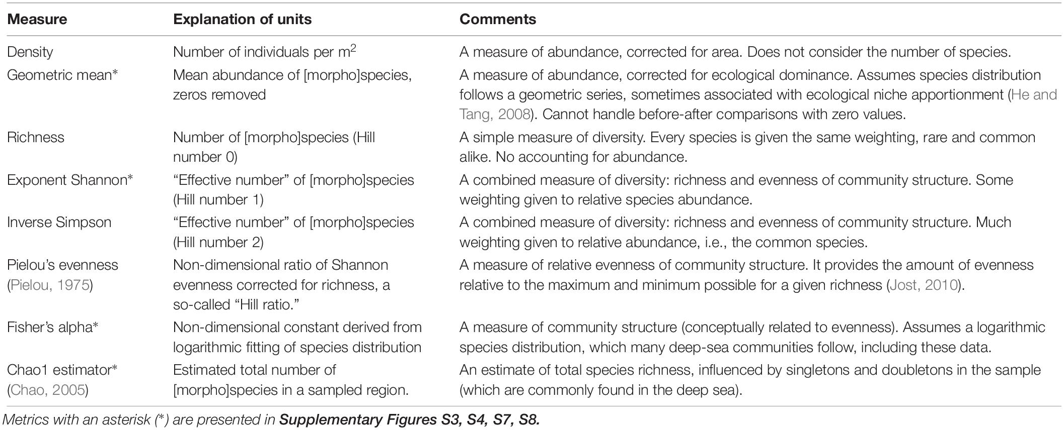
Table 1. Metrics used to detect changes in biodiversity and other ecological properties.

Power Analyses

The statistical power of detecting changes from the baseline condition was calculated for each treatment and measure. Custom R scripts (R Core Team, 2018) – using the “vegan” package (Oksanen et al., 2016) and the “pwr” package (Champely et al., 2018) – simulated degradation, while calculating the metrics and their statistical power (our R code is provided in Supplementary Materials, section S1.4.).

The number of sampling sites required to reliably detect a treatment is dependent upon the magnitude of the stressors being measured, the metric, sample size, and desired error thresholds (type I and type II). For each of the degradation treatments and metrics, power analyses were conducted, using two-tailed t-tests with a significance of 0.05 and confidence levels (avoidance of type II error) of 80, 90, and 95%. Statistical effect size was calculated for each treatment and measure, using Cohen’s d, corrected for using sampled data. (Cohen’s d is the difference between two means divided by their pooled standard deviation.) As that megafaunal sub-sample sizes were larger here than what historically has been collected, Hedge’s g was not used to correct for small samples as had been done in an earlier meta-analysis (Jones et al., 2017).

Sub-Sampling Size and Replication

Drawing from the larger dataset with replacement, 2000 random sub-samples were created for each of the nine degradation treatments for a range of surveyed area sizes. Regarding the size of the sub-samples, Simon-Lledó et al. (2019a) note that when using the same APEI-6 data set as here, stable estimation of biodiversity-related parameters was extremely variable. For example, estimation of mean richness required the largest sub-sample size to plateau (>1000 individuals) while density required the smallest (>30 individuals). Arithmetic mean within sample dissimilarity (autosimilarity) required sub-sample sizes >250 individuals to stabilise, whereas mean exponent Shannon stabilised with sub-sample sizes >350 individuals. Based on these results, and upon the expectation that the abundance of individuals will decline after degradation treatments, starting sub-samples of 250, 500, 750, and 1000 individuals were explored.

Consideration was also given to developing methods that could be cost-effectively applied in commercial operations, and for that reason it was decided to use fixed-area replicates, rather than fixed-abundance replicates, which require greater survey effort and post hoc processing. Calibration runs were used to translate the desired numbers of individuals into fixed-area sub-samples (Table 2).

TABLE 2

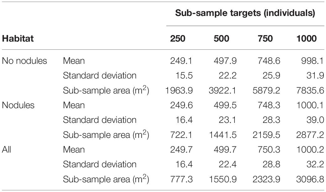
Table 2. Mean number of individuals, standard deviation, and mean area of sub-samples, across 2000 randomisations.

Results

In our simulations of impacts, using deep-sea data from the CCZ ensured that the salient mathematical properties of its deep-sea species distributions were captured in the measurements; namely, the log-linear rank abundance distribution, low density (on average < 0.33 ind. m^–2), high [morpho]species richness (which did not plateau at any of the sub-sample sizes, indicating that morphospecies richness was not fully characterised in any of the sample unit sizes used), and the “long tail” of singletons, doubletons, and tripletons that accounted for more than one-third of all observations within the study area (>18,000 m²) (c.f. Supplementary Figures S1, S2 and Supplementary Table S1; Tilot, 2006; Amon et al., 2016; Durden et al., 2016; Jones et al., 2017; Simon-Lledó et al., 2019a).

Degradation Treatments

The eight degradation treatments caused a wide range of impacts; morphospecies abundance can be reduced by more than 75%, and morphospecies richness by nearly 40% (Table 3). As might be expected, the nodule affinity stressors, which affected only a subset of morphospecies, had less of a detectable impact than the broader stochastic areal treatments (Figure 1). As intended in the numerical model, their combined effect is greater than the sum of their separate effects (Table 3). Initial impacts by just one stressor alone are more difficult to detect, but then emerge when the second stressor is applied, increasing rapidly when either stressor is increased. This can be seen in the transition from a 26% stochastic areal stressor alone (notated as “0 + 26a” per Table 3) to when a 25% nodule affinity stressor is added to it (“25n + 26a”; Table 3). In the case of sub-samples starting with 750 individuals, the first stressor reduces mean abundance to about 709 individuals (-5.5%), but the introduction of the second stressor reduces it further to about 574 individuals (-23.5%). In this example, morphospecies richness has declined from 79 (baseline) to 78 to 76. However, the addition of any further stressor, reduces morphospecies richness much more, to 69, then 61, 58, and 53 (Figure 1).

TABLE 3

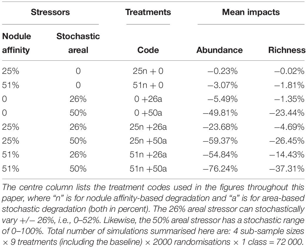
Table 3. The degradation treatments and their mean impacts on abundance and morphospecies richness, across the four sub-sample sizes (250, 500, 750, 1000 individuals), without differentiating habitat (i.e., the “All” class).

FIGURE 1

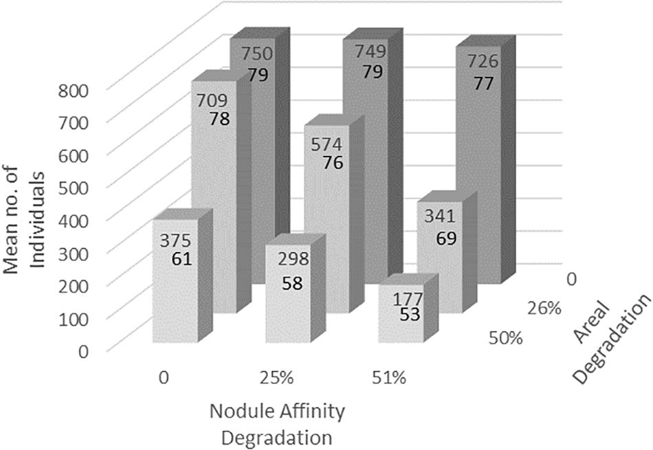
Figure 1. Example of impacts of the degradation treatments on mean abundance (upper number) and mean morphospecies richness (lower number), for 2000 sub-samples calibrated to contain approximately 750 individuals initially (y-axis). For simplicity, just the “All” class is shown, i.e., without any data stratification. Note that the nodule affinity stressor alone (x-axis, back row of dark columns) has little or no impact, but that its influence becomes apparent when combined with the stochastic areal stressor (z-axis). These two different “StressorFactors” (in percent) and how they were applied, are described in section Materials and methods.

The impacts associated with the (25n+26a) treatment presage increased losses of morphospecies (i.e., local extirpations), should the simulated stressors continue to increase. We focus on this treatment in particular when considering the properties of the various metrics below, as a simulated “tipping point.”

Losses of abundance and morphospecies can be readily measured through density and richness, respectively. However, richness is a relatively insensitive measure as it requires complete removal of a species to detect a change. Six metrics more sensitive to ongoing changes were also considered. Of these, exponent Shannon, inverse Simpson, Pielou’s evenness, and Fisher’s alpha each take into account both density and richness. Perhaps counter-intuitively, these four metrics at first generally increase as the stressors used in this analysis increase, before dropping off again. This is because the stressors tended to impact the more abundant morphospecies that are more widespread, many of which are also associated with nodules (e.g., porifera). Reducing the dominance of the most common morphospecies increased evenness and hence the heterogeneity diversity metrics increased. When No-Nodule and Nodule classes are separated out, the effect is further heightened in the Nodule class owing to the nodule affinity stressor, and dampened in the No-Nodule class, as would be expected (Figure 2).

FIGURE 2

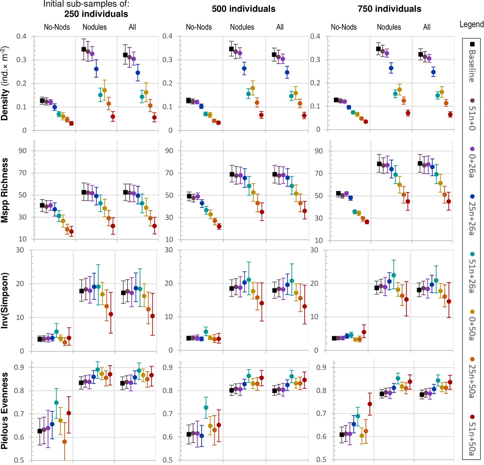
Figure 2. Seven degradation treatments (plus baseline) across three sub-sample sizes (250, 500, 750 individuals), captured using four metrics: density, morphospecies richness, inverse Simpson, and Pielou’s evenness (leftmost labels). The treatment codes in the rightmost legend are explained in Table 3. They are ordered according to increasing combined impacts left to right, violet to red. Error bars depict the 95% range of results (a proxy for confidence) over 2000 simulations. One of the treatments (25n + 0) is not displayed because in isolation it had very little impact. Sub-samples of 1000 individuals performed very, similarly, to 750 and are therefore not shown. Four additional metrics are displayed in Supplementary Figure S3.

Exponent Shannon and inverse Simpson perform very, similarly, across all treatments. As impacts increase and richness drops, Pielou’s evenness, being a measure of evenness corrected for richness, does not decline like the other metrics, but stays at a value higher than the baseline throughout the treatment regime, suggesting a change to the “ecological balance” of the data, i.e., a flattening (and foreshortening) of the log-linear rank abundance distribution of the morphospecies (Supplementary Figure S1). It has generally less variability across randomisations (narrower error bars) than the three other related metrics, with Fisher’s Alpha being the most variable (Figure 2 and Supplementary Figures S3, S5, S7).

The remaining two metrics considered here, geometric mean of morphospecies abundance and the Chao1 estimator, are alternative ways to measure abundance and richness, respectively. They both decline steadily under the treatment regime. Having greater variability, however, neither measure appears to provide any additional information to what is already captured in the simpler metrics of density and richness (compare Figure 2 and Supplementary Figure S3).

Given the lethal nature of the simulations on individuals, changes in density were most apparent, as would be expected. Unlike the other metrics, changes in density were readily detectable at lower impact treatments [e.g., (0 + 26a)] across all sub-sample sizes, even the smallest (250 individuals). Density was the only measure that was significantly different (i.e., at or outside the 95% error bars) across all habitat classes. Although not a biodiversity metric per se, changes in total density preceded broader impacts upon biodiversity yet to come. Treatments more severe than the (0 + 26a) treatment [i.e., (25n + 26a] and greater) were detected by all eight of the metrics (Figure 2). However, unlike density, their power of detection is not visually obvious from the plots, and power analysis is required.

Power Analyses

As would be expected, the larger impacts require fewer monitoring sites to be detected. Also as expected, larger area monitoring sites (i.e., sub-samples with more individuals) produce less variability than smaller ones, and require fewer replicates, though the relationship is non-linear. The statistical effect size varied according to treatments, sub-sample size, and metrics. For example, the (25n + 26a) treatment, “All” class, with sub-samples of 250 individuals, Cohen’s d was about -3.86 with regard to density, 1.80 for Pielou’s evenness, and -0.78 for richness (Table 5).

As noted above, density requires the fewest sites to detect changes in abundance (usually 3 is sufficient; Figure 3), though its ecological interpretation is limited because it does not detect compositional changes. Richness, which does detect compositional change, is unable to detect early declines when a given morphospecies is still present. For the (25n + 26a) treatment, for example, richness declined only about 5%, and thus about 24 replicates would be required to detect that change (significance ≤0.05, confidence ≥95%; sub-sample size of 750 individuals; Figure 3).

FIGURE 3

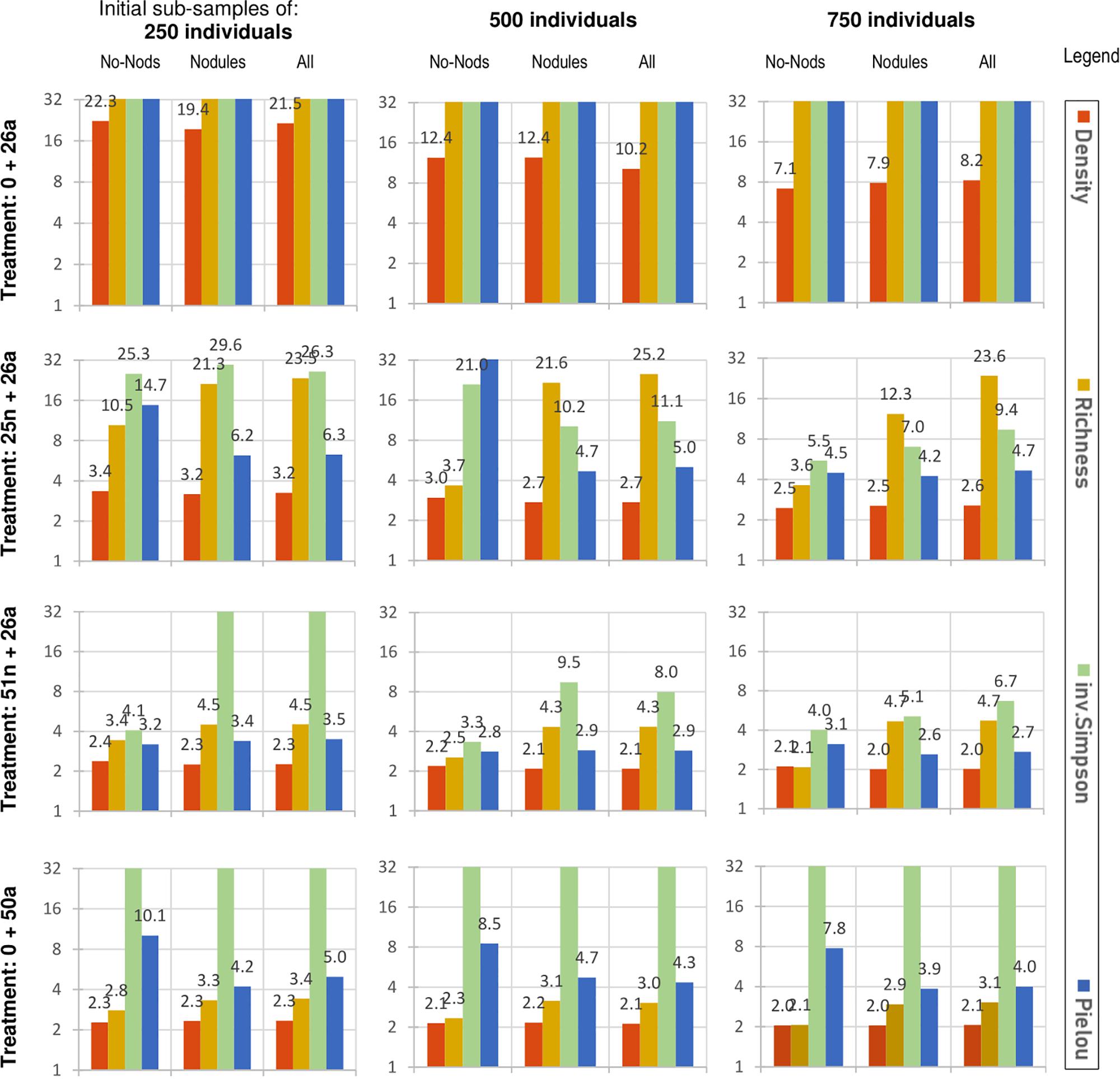
Figure 3. Power analysis of the four metrics in Figure 2 above (rightmost labels), across three initial sub-sample sizes (250, 500, 750), under the four middle degradation treatments (leftmost legend, explained in Table 3), increasing in severity from top to bottom. Two-tailed t-test error thresholds: significance ≤0.05; power (type II confidence) ≥95%. The y-axis is logarithmic, depicting the theoretical number of sampling sites required to meet these error thresholds (≥2). Values greater than 32 are not fully displayed, as they would be impractical to implement. Additional metrics are displayed in Supplementary Figures S3, S4.

In detecting compositional change before [morpho]species are lost, exponent Shannon and inverse Simpson perform similarly. To detect the (25n + 26a) treatment, about 10 sites (of 750 individuals) are required –as compared to the more than 20 required by the richness measure. However, detecting change in evenness alone, using Pielou’s evenness, requires half that again (∼5; Figure 3 and Supplementary Figure S4).

Increasing the confidence from 80 to 95% often means adding only one more monitoring site (Table 4). The effect of sub-sample size is often non-linear, i.e., the power gained through using large monitoring sites of 1000 individuals is not usually twice as great as for 500 (though see exponent Shannon, Table 4). The statistical effect size, per Cohen’s d, increases for most metrics (except richness) as sub-sample size increases (Table 5).

TABLE 4

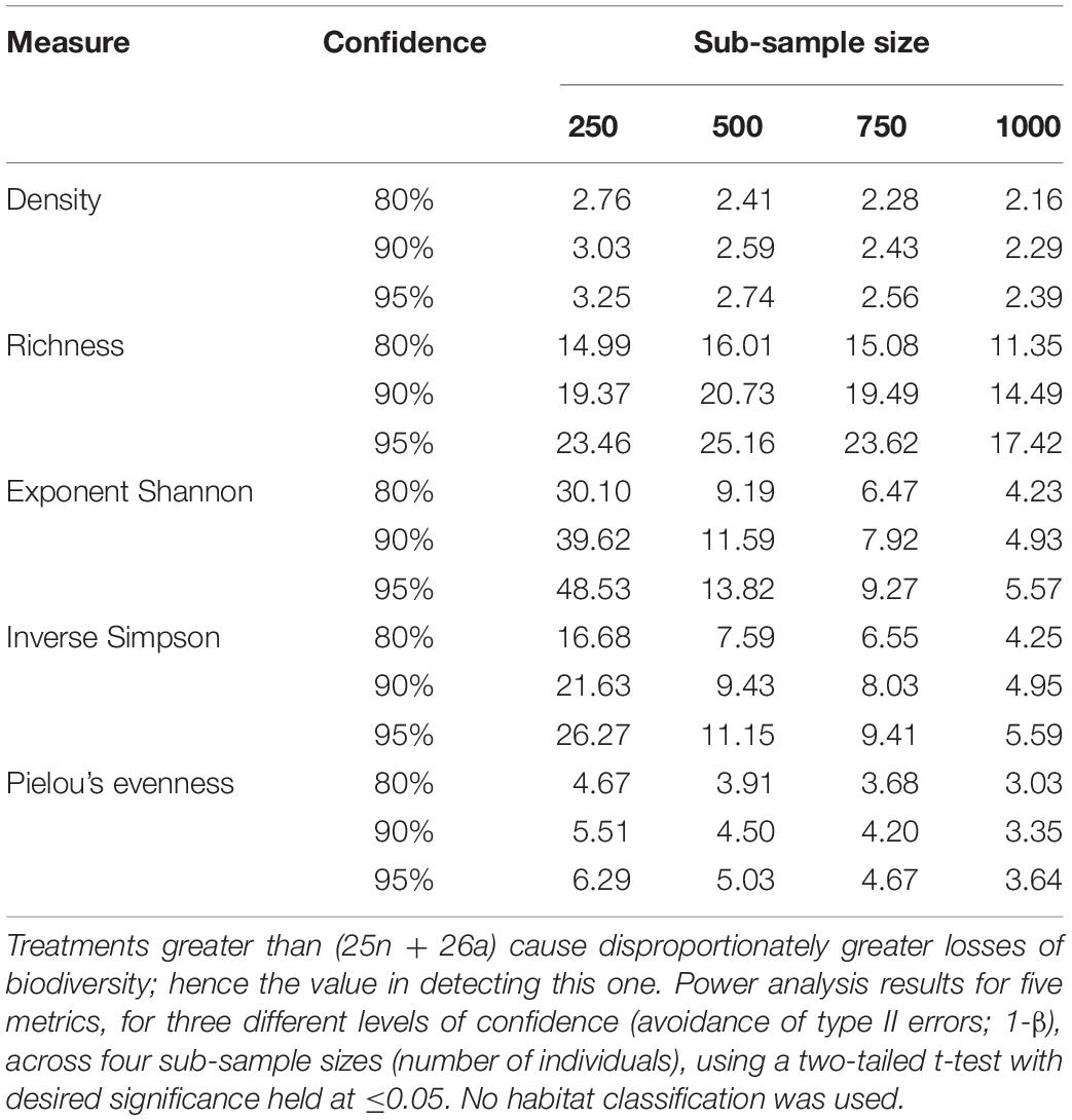
Table 4. Number of monitoring sites required to detect the (25n + 26a) treatment as compared to the baseline.

TABLE 5

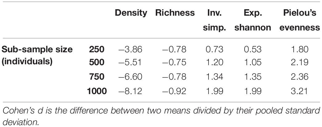
Table 5. Cohen’s d, a measure of effect size, for the (25n + 26a) treatment, for five different metrics across four sub-sample sizes.

Impacts to Different Habitats

Some habitat-specific impacts were observed. For example, the (51n + 26a) treatment is much more easily detected for the Flats habitat (which has the highest density of nodules) than for Troughs or Ridges (Pielou’s evenness and inv. Simpson, Supplementary Figure S5).

Usually, the addition of classes means additional monitoring sites (Figure 3 vs. Supplementary Figures S6, S8). An exception is richness. For the (25n + 26a) treatment, with sub-samples of 750 individuals, the two-part classification based on no-nodules/nodules requires 12.3 sites (nodules class) plus 3.6 (no-nodules class) totalling to 15.9 sites in all. No classification (“All”) requires 23.6. Hence, in this example, using this two-part classification would be more cost effective. However, if smaller sub-samples of 500 individuals are used, this economy is lost, and the total number of sites require is approximately the same with or without the classification (∼25; Figure 3, 3rd row).

Discussion

To reliably detect the impacts of polymetallic nodule mining, before serious harm occurs, our results suggest the use of impact monitoring sampling unit sizes of at least 500–750 individuals each and a minimum replication of five of such samples collected in both disturbed and control sites. In the northeast CCZ, this translates to approximately 1500–2300 m² per impact monitoring site, i.e., 7500–11,500 m² of seafloor surveyed in total for reliable detection of disturbance-mediated variations in megabenthic features at a local scale. These particular details will change if different licence areas in the CCZ have different megafaunal species distributions. However, the approach and choice of metrics presented here should remain relevant. For example, while the community composition and species present will indeed vary from place to place or time to time, total macroecological metrics tend to vary less than those that are species specific (e.g., Ernest et al., 2008, 2009; Ruhl et al., 2014). Ecological parameters such as numerical density and Pielou’s evenness can be used to track loss of abundance and changes to some aspects of community structure (evenness), respectively. If severe damage occurs, the more readily communicated and understood metric of richness can also be used to help characterise it, however, richness is unable to detect early warnings before species extirpation occurs.

Larger sampling unit sizes typically yield more accurate characterisations of biological communities (Gotelli and Colwell, 2001). Here, the smallest sub-sample size considered (250 individuals) displayed disproportionately greater variability across metrics, making detection of the smaller impacts more difficult (i.e., of lower statistical power), and therefore cannot be recommended. Furthermore, effect size usually increased with sample unit size; hence the treatments became more detectable as sample unit size increased.

Increasing the desired confidence from 80 to 95% often required just one more monitoring site. Because a false negative result could mean that harmful impacts are not detected, the more precautionary 95% confidence threshold is recommended here, as displayed in the results (Figure 3 and Supplementary Figures S4, S6, S8).

In our simulations, two commonly used measures of “diversity” (exponent Shannon and inverse Simpson) both increased under initial degradation treatments, before declining. No new species were added; rather, the measures increased solely as a result of increased evenness. For this reason, Pielou’s evenness, which separates out evenness from richness (Jost, 2010), was more sensitive in detecting this change than all the other diversity measures tested. Because our simulations show that commonly used metrics of biodiversity may increase initially when measuring the impacts of DSM on deep-sea communities, there is the possibility that they could be misinterpreted, perhaps as indicating some sort of “intermediate disturbance” benefit (Connell, 1978). While it is possible that intermediate disturbance may increase richness in reality, through creation of a patch mosaic of conditions promoting settlement of a greater range of species (Grassle and Sanders, 1973), the extremely low recolonisation rates expected in the CCZ and lack of obvious r-selected species (Jones et al., 2017, 2018b), would make it unlikely.

Although lower levels of the simulated stressors in isolation were difficult to detect, requiring many replicates, their statistical effect sizes would suggest that they could still be simulating ecologically important stress, likely to have (perhaps sub-lethal) consequences. For example, the (0+26a) treatment still had what is commonly called a “medium” effect size (d = 0.42) when measured using Pielou’s evenness (sub-samples of 750). However, its reliable detection (p = 0.5, 1-β = 0.95) would require 77 replicate sites –a number that would be very costly to implement in the CCZ. Indeed, many of the metrics tested here required more than 32 replicates to detect the (simulated) impacts, which in the context of the deep sea is likely to be argued as being too expensive to economically justify their usage (e.g., those measures in Supplementary Figures S3, S4, S7, S8).

It has not yet been determined what is an acceptable effect size for deep-sea ecology. Long-term results from historical studies typically yield results around 1, with 2 not being unusual (Jones et al., 2017). However, in other fields, these effects would be characterised as large or even huge. In developing his measure for the field of psychology, Cohen (1988) suggested that an absolute value of d = 0.2 be considered a “small” effect size, 0.5 represents a “medium” effect size, and 0.8 a “large” effect size. Sawilowsky (2009) expanded upon this, suggesting that 1.2 is “very large,” and greater than 2 is “huge.” Thus, for the (25n + 26a) treatment, the effect on richness could be characterised as “large”; on evenness (as measured by Pielou’s measure) as approaching “huge”; and density as off the scale. If sub-sample size is increased, the effect size also increases, such that for sub-samples of 1000, all metrics in Table 5, except richness, are now “huge.” However, owing to the low density of organisms and inherent variability of the CCZ data, several replicates are still required to detect these “huge” changes (Table 4).

Determining analogous early warnings in real-world DSM is yet to be done. The results presented here, which simulate possible threshold effects, should be seen as indicative. Given that Cohen’s d was already very large for some metrics, translating actual ecosystem effects into statistical effect sizes should be seen as a priority area for future research. For deep-sea benthic ecosystems, a global study of 116 sites found that deep-sea ecosystem functioning is exponentially related to deep-sea biodiversity and that ecosystem efficiency is also exponentially linked to functional biodiversity (Danovaro et al., 2008). In the CCZ it is thus conceivable that a small loss of benthic richness could actually translate to a much greater loss of ecosystem efficiency and functionality. Total density and diversity measures represent a first step in monitoring. However, should they pass a threshold value, further analysis could be triggered, including the identification of particularly impacted species. The use of indicator species is widely used in understanding change in managed areas and this concept could be added to track a limited number of taxa with better baseline knowledge of their ecology and variation. The choice of suitable indicator taxa requires further research.

Although benthic metazoan megafauna are just one aspect of deep-sea ecological communities, they are an important part of nodule-dominated systems, readily surveyed through ROV and AUV photography or videography. If deposition of plumes does indeed occur in areas adjacent to DSM operations, then megafauna, particularly the filter feeders, are likely to be particularly affected. However, the detection of change will depend, in part, on the resolution of the camera employed. Lower resolution equipment than used here would require larger samples and greater replication to achieve similar results. Likewise, higher quality equipment could reduce these requirements.

The treatments used here are simplistic in that only the survival / mortality of observed individuals was simulated. Non-lethal injuries that could affect the growth, feeding, reproduction, or other factors affecting the long-term health of an ecological community were not simulated. The importance of measuring sub-lethal effects is well recognised for other offshore industries (e.g., Hughes et al., 2010; Trannum et al., 2011), and deserves further attention in the DSM context. In order to be comprehensive, a DSM monitoring plan will also need to consider a much wider range of species, scales, and impacts than what has been presented here (Jones et al., 2017, 2018a). However, the same techniques could be applied in their monitoring. An understanding of natural variability (e.g., species turnover rates, etc.) will be necessary through the use of control sites (called “Preservation Reference Zones” in ISA nomenclature) to better separate out mining impacts from natural changes (Jones et al., 2018a). If the use of control sites indicates that some areas are undergoing changes that are detectable at the time scale of local mining activities, then more replicates would be required to achieve a comparable level of statistical power. For other terrains and resource types, such as seafloor massive sulphides, the detectability of organisms would likely differ, though the analytical techniques would remain the same. Desktop simulations such as ours can, and should, be improved by in situ DSM experiments and monitoring.

The International Seabed Authority has an obligation to prevent, reduce and control deleterious effects arising from DSM, before serious harm occurs. Additionally, nation states are to avoid interference with the ecological balance of the marine environment. The metrics tested here have been demonstrated to detect changes to both “balance” (evenness) and abundance, which are likely to form part of any such assessment. Future discussions would benefit from a quantification of harm, that can be understood, properly evaluated and compared between studies. This would enable much clearer guidance for contractors on what is the nature of serious harm. Statistical effect sizes are commonly used for this purpose. However, as demonstrated here, effect size will vary depending upon the nature of the impact, sample size, and the metric being used to detect it. Therefore, regulatory thresholds will need to be linked to the details of the monitoring regime.

Regulations of this new industry will need to recognise that detection of impacts before serious harm occurs requires the reliable detection of impacts that are less than serious. Evaluation of statistical power in assessment of monitoring plans proposed by contractors to the ISA can move the assessment of less-than-serious harm towards a more repeatable and objective format. However, monitoring plans submitted to date have either not been made publicly available or have not been detailed enough to determine their statistical properties. Thus, the power of current and proposed monitoring plans to measure impacts, and at what level, is unknown. Furthermore, the criteria and assessments of the ISA’s responsible committee (Legal and Technical Commission) have also not been made publicly available, leaving unanswered whether the proposed monitoring plans are statistically adequate (Ardron, 2018; Ardron et al., 2018). Making monitoring details available, including power analyses, would help facilitate independent review and informed policy discussions.

Scientists, amongst others, have expressed concern over possible ecological impacts of commercial scale DSM (e.g., Wedding et al., 2015; Van Dover et al., 2017). As that deep-seabed resources beyond national jurisdictions are legally the “common heritage of mankind” (United Nations Convention on the Law of the Sea [UNCLOS], 1982), there is a need for international bodies (e.g., the ISA or the United Nations) to determine what level of impact is acceptable to society more broadly (Jaeckel et al., 2017).

This study simulates the comparison of initial baseline assessment information (“before”) with subsequent adjacent mining impacts (“after”) to explore how commonly used metrics of biodiversity respond in the context of morphospecies distributions found in the CCZ. Our recommendations, as discussed above, are summarised in Table 6.

TABLE 6

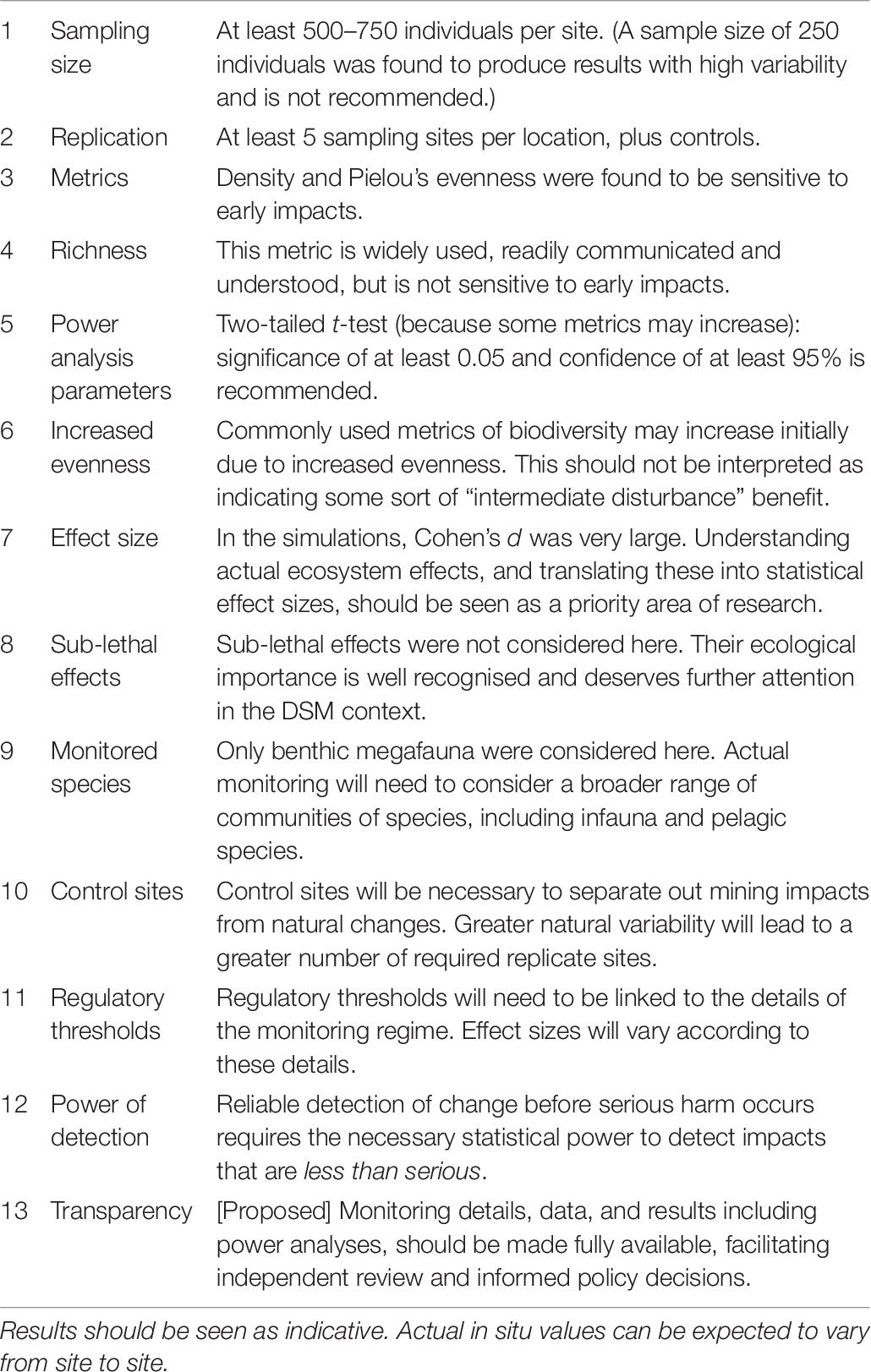
Table 6. Summary of findings and recommendations (in the order presented in section Discussion).

Data Availability Statement

The data used in this paper are presented in Simon-Lledó et al. (2019a) (Table 2), with related analyses uploaded to Pangea: https://doi.pangaea.de/10.1594/PANGAEA.893220.

Author Contributions

JA, HR, and DJ conceptualised the study. JA designed the simulations. JA wrote the R code, incorporating some code written by ES-L from another study. JA analysed the results and wrote the manuscript with contributions from DJ, HR, and ES-L. DJ and ES-L participated in the earlier research cruise which collected the data. ES-L previously processed and analysed the morphospecies and geomorphic classes of the photo data (published elsewhere).

Funding

The research leading to these results has received funding from the European Union Seventh Framework Programme (FP7/2007-2013) under the Managing Impacts of Deep Sea Resource Exploitation (MIDAS) project, Grant agreement 603418. Funding was also provided from the UK Natural Environment Research Council through National Capability funding to NOC (Grant NE/R015953/1) and the Commonwealth Marine Economies Program. The camera survey system used to collect the data in the study was made possible by the Autonomous Ecological Surveying of the Abyss project (Natural Environment Research Council Grant NE/H021787/1).

Conflict of Interest

The authors declare that the research was conducted in the absence of any commercial or financial relationships that could be construed as a potential conflict of interest.

Acknowledgments

We would like to thank the three reviewers for their insightful, thorough, and at times challenging comments. JA would like to thank his long-suffering partner for all the weekends that were not spent doing something enjoyable together.

Supplementary Material

The Supplementary Material for this article can be found online at: https://www.frontiersin.org/articles/10.3389/fmars.2019.00604/full#supplementary-material

References

Aleynik, D., Inall, M. E., Dale, A., and Vink, A. (2017). Impact of remotely generated eddies on plume dispersion at abyssal mining sites in the Pacific. Sci. Rep. 7:16959. doi: 10.1038/s41598-017-16912-2

PubMed Abstract | CrossRef Full Text | Google Scholar

Amon, D. J., Ziegler, A. F., Dahlgren, T. G., Glover, A. G., Goineau, A., Gooday, A. J., et al. (2016). Insights into the abundance and diversity of abyssal megafauna in a polymetallic-nodule region in the eastern clarion-clipperton zone. Sci. Rep. 6:30492. doi: 10.1038/srep30492

PubMed Abstract | CrossRef Full Text | Google Scholar

Amon, D. J., Ziegler, A. F., Drazen, J. C., Grischenko, A. V., Leitner, A. B., Lindsay, D. J., et al. (2017). Megafauna of the UKSRL exploration contract area and eastern Clarion-Clipperton Zone in the Pacific Ocean: Annelida, Arthropoda, Bryozoa, Chordata, Ctenophora, Mollusca. Biodivers. Data J. 5:e14598. doi: 10.3897/BDJ.5.e14598

PubMed Abstract | CrossRef Full Text | Google Scholar

Ardron, J. A. (2018). Transparency in the operations of the International seabed authority: an initial assessment. Mar. Policy 95, 324–331. doi: 10.1016/j.marpol.2016.06.027

CrossRef Full Text | Google Scholar

Ardron, J. A., Ruhl, H. A., and Jones, D. O. (2018). Incorporating transparency into the governance of deep-seabed mining in the area beyond national jurisdiction. Mar. Policy 89, 58–66. doi: 10.1016/j.marpol.2017.11.021

CrossRef Full Text | Google Scholar

Bluhm, H. (2001). Re-establishment of an abyssal megabenthic community after experimental physical disturbance of the seafloor. Deep Sea Res. Part II: Top. Stud. Oceanogr. 48, 3841–3868. doi: 10.1016/s0967-0645(01)00070-4

CrossRef Full Text | Google Scholar

Bo, M., Bava, S., Canese, S., Angiolillo, M., Cattaneo-Vietti, R., and Bavestrello, G. (2014). Fishing impact on deep Mediterranean rocky habitats as revealed by ROV investigation. Biol. Conserv. 171, 167–176. doi: 10.1016/j.biocon.2014.01.011

CrossRef Full Text | Google Scholar

Boschen, R. E., Rowden, A. A., Clark, M. R., Barton, S. J., Pallentin, A., and Gardner, J. P. A. (2015). Megabenthic assemblage structure on three New Zealand seamounts: implications for seafloor massive sulfide mining. Mar. Ecol. Prog. Ser. 523, 1–14. doi: 10.3354/meps11239

CrossRef Full Text | Google Scholar

Burns, R. E. (1980). Assessment of environmental effects of deep ocean mining of manganese nodules. Helgol. Meeresunters 33, 433–442. doi: 10.1007/BF02414768

CrossRef Full Text | Google Scholar

Champely, S., Ekstrom, C., Dalgaard, P., Gill, J., Weibelzahl, S., Anandkumar, A., et al. (2018). R Package ‘pwr’. Available at: https://github.com/heliosdrm/pwr (accessed September, 2019).

Google Scholar

Chao, A. (2005). “Species estimation and applications,” in Encyclopedia of Statistical Sciences, 2nd Edn, eds S. Kotz, N. Balakrishnan, C. B. Read, and B. Vidakovic, (New York, NY: Wiley).

Google Scholar

Chao, A., Chiu, C.-H., and Jost, L. (2010). Phylogenetic diversity metrics based on Hill numbers. Philos. Trans. R. Soc. B 365, 3599–3609. doi: 10.1371/journal.pone.0105818

PubMed Abstract | CrossRef Full Text | Google Scholar

Chao, A., and Jost, L. (2012). “Diversity metrics,” in Encyclopedia of Theoretical Ecology, eds A. Hastings, and L. Gross, (Berkeley: University of California Press), 203–207.

Google Scholar

Cohen, J. (1988). Statistical Power Analysis for the Behavioral Sciences. Abingdon,: Routledge.

Google Scholar

Connell, J. H. (1978). Diversity in tropical rain forests and coral reefs. Science 199, 1302–1310. doi: 10.1126/science.199.4335.1302

PubMed Abstract | CrossRef Full Text | Google Scholar

Dahlgren, T., Wiklund, H., Rabone, M., Amon, D., Ikebe, C., Watling, L., et al. (2016). Abyssal fauna of the UK-1 polymetallic nodule exploration area, clarion-clipperton zone, central pacific ocean: cnidaria. Biodivers. Data J. 4, e9277. doi: 10.3897/BDJ.4.e9277

PubMed Abstract | CrossRef Full Text | Google Scholar

Danovaro, R., Gambi, C., Dell’Anno, A., Corinaldesi, C., Fraschetti, S., Vanreusel, A., et al. (2008). Exponential decline of deep-sea ecosystem functioning linked to benthic biodiversity loss. Curr. Biol. 18, 1–8. doi: 10.1016/j.cub.2007.11.056

PubMed Abstract | CrossRef Full Text | Google Scholar

Durden, J. M., Schoening, T., Althaus, F., Friedman, A., Garcia, R., Glover, A. G., et al. (2016). “Perspectives in visual imaging for marine biology and ecology: from acquisition to understanding,” in Oceanography and Marine Biology: An Annual Review, Vol. 54, eds R. N. Hughes, D. J. Hughes, I. P. Smith, and A. C. Dale, (Boca Raton, FL: CRC Press), 1–72.

Google Scholar

Ernest, S. K., Brown, M. J. H., Thibault, K. M., White, E. P., and Goheen, J. R. (2008). Zero sum, the niche, and metacommunities: long-term dynamics of community assembly. Am. Nat. 172, E257–E269. doi: 10.1086/592402

PubMed Abstract | CrossRef Full Text | Google Scholar

Ernest, S. K. M., White, E. P., and Brown, J. H. (2009). Changes in a tropical forest support metabolic zero-sum dynamics. Ecol. Lett. 12, 507–515. doi: 10.1111/j.1461-0248.2009.01305.x

PubMed Abstract | CrossRef Full Text | Google Scholar

Glasby, G. P. (2000). Lessons learned from deep-sea mining. Science 289, 551–553. doi: 10.1126/science.289.5479.551

PubMed Abstract | CrossRef Full Text | Google Scholar

Glover, A., Wiklund, H., Rabone, M., Amon, D., Smith, C., O’Hara, T., et al. (2016). Abyssal fauna of the UK-1 polymetallic nodule exploration claim, clarion-clipperton zone, central pacific ocean: echinodermata. Biodivers. Data J. 4, e7251–e7251. doi: 10.3897/BDJ.4.e7251

PubMed Abstract | CrossRef Full Text | Google Scholar

Gotelli, N. J., and Colwell, R. K. (2001). Quantifying biodiversity: procedures and pitfalls in the measurement and comparison of species richness. Ecol. Let. 4, 379–391. doi: 10.1046/j.1461-0248.2001.00230.x

CrossRef Full Text | Google Scholar

Grassle, J. F., and Sanders, H. L. (1973). Life histories and the role of disturbance. Deep Sea Res. 20, 643–659. doi: 10.1016/0011-7471(73)90032-6

CrossRef Full Text | Google Scholar

Grassle, J. F., Sanders, H. L., Hessler, R. R., Rowe, G. T., and McLellan, T. (1975). Pattern and zonation: a study of the bathyal megafauna using the research submersible alvin. Deep Sea Res. 22, 457–481. doi: 10.1016/0011-7471(75)90020-0

CrossRef Full Text | Google Scholar

He, F., and Tang, D. (2008). Estimating the niche preemption parameter of the geometric series. Acta Oecol. 33, 105–107. doi: 10.1016/j.actao.2007.10.001

CrossRef Full Text | Google Scholar

Hill, M. O. (1973). Diversity and evenness: a unifying notation and its consequences. Ecology 54, 427–431.

Google Scholar

Hughes, S. J. M., Jones, D. O. B., Hauton, C., Gates, A. R., and Hawkins, L. E. (2010). An assessment of drilling disturbance on echinus acutus var. norvegicus based on in-situ observations and experiments using a remotely operated vehicle (ROV). J. Exp. Mar. Biol. Ecol. 395, 37–47. doi: 10.1016/j.jembe.2010.08.012

CrossRef Full Text | Google Scholar

Jaeckel, A., Gjerde, K. M., and Ardron, J. A. (2017). Conserving the common heritage of humankind – options for the deep seabed mining regime. Mar. Policy 78, 150–157. doi: 10.1016/j.marpol.2017.01.019

CrossRef Full Text | Google Scholar

Jones, D. O. B., Bett, B. J., Wynn, R. B., and Masson, D. G. (2009). The use of towed camera platforms in deep-water science. Underwater Technol. 28, 41–50. doi: 10.3723/ut.28.041

CrossRef Full Text | Google Scholar

Jones, D. O. B., Gates, A. R., and Lausen, B. (2012). Recovery of deep-water megafaunal assemblages from hydrocarbon drilling disturbance in the faroe-shetland channel. Mar. Ecol. Prog. Ser. 461, 71–82. doi: 10.3354/meps09827

CrossRef Full Text | Google Scholar

Jones, D. O. B., Kaiser, S., Sweetman, A. K., Smith, C. R., Menot, L., Vink, A., et al. (2017). Biological responses to disturbance from simulated deep-sea polymetallic nodule mining. PLoS One 12:e0171750. doi: 10.1371/journal.pone.0171750

PubMed Abstract | CrossRef Full Text | Google Scholar

Jones, D. O. B., Ardron, J. A., Colaço, A., and Durden, J. M. (2018a). Environmental considerations for impact and preservation reference zones for deep-sea polymetallic nodule mining. Mar. Policy. doi: 10.1016/j.marpol.2018.10.025

CrossRef Full Text | Google Scholar

Jones, D. O. B., Amon, D. J., and Chapman, A. S. A. (2018b). Mining deep-ocean mineral deposits: what are the ecological risks? Elements 14, 325–330. doi: 10.2138/gselements.14.5.325

CrossRef Full Text | Google Scholar

Jost, L. (2006). Entropy and diversity. OIKOS 113, 363–375. doi: 10.1111/j.2006.0030-1299.14714.x

CrossRef Full Text | Google Scholar

Jost, L. (2010). The relation between evenness and diversity. Diversity 2, 207–232. doi: 10.3390/d2020207

CrossRef Full Text | Google Scholar

JPI Oceans, (2018). MiningImpact: Environmental Impacts and Risks of Deep-Sea Mining. Available at: https://miningimpact.geomar.de/home (accessed September, 2019).

Google Scholar

Levin, L. A., Mengerink, K., Gjerde, K. M., Rowden, A. A., Van Dover, C. L., Clark, M. R., et al. (2016). Defining “serious harm” to the marine environment in the context of deep-seabed mining. Mar. Policy 74, 245–259. doi: 10.1016/j.marpol.2016.09.032

CrossRef Full Text | Google Scholar

Lutz, M. J., Caldeira, K., Dunbar, R. B., and Behrenfeld, M. J. (2007). Seasonal rhythms of net primary production and particulate organic carbon flux to depth describe the efficiency of biological pump in the global ocean. J. Geophys. Res. 112, C10011.

Google Scholar

MIDAS, (2016). Managing Impacts of Deep-Sea Resource Exploitation. Available at: Available at: https://www.eu-midas.net/ (accessed September, 2019).

Google Scholar

Miljutin, D., Miljutina, M., Arbizu, P., and Galéron, J. (2011). Deep-sea nematode assemblage has not recovered 26 years after experimental mining of polymetallic nodules (clarion-clipperton fracture zone, tropical eastern pacific). Deep Sea Res. Part I: Oceanogr. Res. Pap. 58, 885–897. doi: 10.1016/j.dsr.2011.06.003

CrossRef Full Text | Google Scholar

Molodtsova, T. N., and Opresko, D. M. (2017). Black corals (Anthozoa: Antipatharia) of the clarion-clipperton fracture zone. Mar. Biodiversi. 47, 349–365. doi: 10.1007/s12526-017-0659-6

CrossRef Full Text | Google Scholar

Morris, K. J., Bett, B. J., Durden, J. M., Huvenne, V. A. I., Milligan, R., Jones, D. O. B., et al. (2014). A new method for ecological surveying of the abyss using autonomous underwater vehicle photography. Limnol. Oceanogr. Methods 12, 795–809. doi: 10.4319/lom.2014.12.795

CrossRef Full Text | Google Scholar

Oebius, H. U., Becker, H. J., Rolinski, S., and Jankowski, J. A. (2001). Parametrization and evaluation of marine environmental impacts produced by deep-sea manganese nodule mining. Deep Sea Res. Part II 48, 3453–3467. doi: 10.1016/s0967-0645(01)00052-2

CrossRef Full Text | Google Scholar

Oksanen, J., Blanchet, F. G., Friendly, M., Kindt, R., Legendre, P., McGlinn, D., et al. (2016). R ‘Vegan’ package. Available at: https://cran.r-project.org (accessed September, 2019).

Google Scholar

Pielou, E. C. (1975). Ecological diversity. New York, NY: John Wiley and Sons.

Google Scholar

R Core Team, (2018). R: A Language and Environment for Statistical Computing. R Foundation for Statistical Computing. Vienna: R Core Team.

Google Scholar

Ruhl, H. A., Bett, B. J., Hughes, S. J. M., Alt, C. J. S., Ross, E. J., Lampitt, R. S., et al. (2014). Links between deep-sea respiration and community dynamics. Ecology 95, 1651–1662. doi: 10.1890/13-0675.1

PubMed Abstract | CrossRef Full Text | Google Scholar

Rühlemann, C., and Knodt, S. (2015). Manganese nodule exploration & exploitation from the deep ocean. J. Ocean Technol. 10, 1–9.

Google Scholar

Sawilowsky, S. (2009). New effect size rules of thumb. J. Mod. Appl. Statist. Methods 8, 467–474.

Google Scholar

Schoening, T., Jones, D. O., and Greinert, J. (2017). Compact-morphology-based poly-metallic nodule delineation. Sci. Rep. 7:13338. doi: 10.1038/s41598-017-13335-x

PubMed Abstract | CrossRef Full Text | Google Scholar

Sibson, R. (1969). Information radius. Zeitschrift für Wahrscheinlichkeitstheorie und verwandte Gebiete 14, 149–160.

Google Scholar

Simon-Lledó, E. (2019). Megabenthic Ecology of Abyssal Polymetallic Nodule Fields. PhD dissertation, University of Southampton, Southampton.

Google Scholar

Simon-Lledó, E., Bett, B. J., Huvenne, V. A. I., Schoening, T., Benoist, N. M. A., Jeffreys, R. M., et al. (2019a). Megafaunal variation in the abyssal landscape of the clarion clipperton zone. Prog. Oceanogr. 170, 119–133. doi: 10.1016/j.pocean.2018.11.003

PubMed Abstract | CrossRef Full Text | Google Scholar

Simon-Lledó, E., Bett, B. J., Huvenne, V. A., Schoening, T., Benoist, N. M., and Jones, D. O. (2019b). Ecology of a polymetallic nodule occurrence gradient: implications for deep-sea mining. Limnol. Oceanogr. 64, 1883–1894. doi: 10.1002/lno.11157

CrossRef Full Text | Google Scholar

Simon-Lledó, E., Bett, B. J., Huvenne, V. A. I., Köser, K., Schoening, T., Greinert, J., et al. (2019c). Simulated deep-sea mining, biological effects after 26 years. Sci. Rep. 9:8040.

Google Scholar

Smith, C. R., Levin, L. A., Koslow, A., Tyler, P. A., and Glover, A. G. (2008). “The near future of the deep seafloor ecosystems,” in Aquatic Ecosystems: Trends and Global Prospects, ed. N. Polunin, (Cambridge: Cambridge University Press), 334–349.

Google Scholar

Stoyanova, V. (2012). “Megafaunal Diversity Associated with Deep-sea Nodule-bearing Habitats in the Eastern Part of the Clarion-Clipperton Zone,” in NE Pacific. 12th International Multidisciplinary Scientific GeoConference. SGEM, (Sofia: Surveying Geology and Mining Ecology Management), 64 5–651.

Google Scholar

Stratmann, T., Lins, L., Purser, A., Marcon, Y., Rodrigues, C. F., Ravara, A., et al. (2018). Abyssal plain faunal carbon flows remain depressed 26 years after a simulated deep-sea mining disturbance. Biogeosciences 15, 4131–4145. doi: 10.5194/bg-15-4131-2018

CrossRef Full Text | Google Scholar

Taboada, S., Riesgo, A., Wiklund, H., Paterson, G. L. J., Koutsouveli, V., Santodomingo, N., et al. (2018). Implications of population connectivity studies for the design of marine protected areas in the deep sea: an example of a demosponge from the clarion-clipperton zone. Mol. Ecol. 27, 4657–4679. doi: 10.1111/mec.14888

PubMed Abstract | CrossRef Full Text | Google Scholar

Tilot, V. (2006). “Biodiversity and distribution of the megafauna Vol.2 Annotated photographic atlas of the echinoderms of the Clarion-Clipperton Fracture Zone,” in Intergovernmental Oceanographic Commission (IOC) of United Nations Educational, (Paris: Scientific and Cultural Organisation), 67.

Google Scholar

Trannum, H. C., Nilsson, H. C., Schaanning, M. T., and Norling, K. (2011). Biological and biogeochemical effects of organic matter and drilling discharges in two sediment communities. Mar. Ecol. Prog. Ser. 442, 23–36. doi: 10.3354/meps09340

CrossRef Full Text | Google Scholar

United Nations Convention on the Law of the Sea [UNCLOS], (1982). Opened for signature 10 Dec 1982 and entered into force 16 Nov 1994; 1833 UNTS 397. Montego Bay: UNCLOS

Google Scholar

Van Dover, C. L., Ardron, J. A., Escobar, E., Gianni, M., Gjerde, K. M., Jaeckel, A., et al. (2017). Biodiversity loss from deep-sea mining. Nat. Geosci. 10, 464–465.

Google Scholar

Vanreusel, A., Hilario, A., Ribeiro, P. A., Menot, L., and Arbizu, P. M. (2016). Threatened by mining, polymetallic nodules are required to preserve abyssal epifauna. Sci. Rep. 6:26808. doi: 10.1038/srep26808

PubMed Abstract | CrossRef Full Text | Google Scholar

Wedding, L. M., Reiter, S. M., Smith, C. R., Gjerde, K. M., Kittinger, J. N., Friedlander, A. M., et al. (2015). Managing mining of the deep seabed. Science 349, 144–145.

Google Scholar