The Development and Validation of a Profiling Glider Deep ISFET-Based pH Sensor for High Resolution Observations of Coastal and Ocean Acidification

Introduction

Ocean acidification (OA) has presented great research challenges and has significant societal ramifications that range from economic losses due to the decreased survival of commercially important organisms to the ecological consequences associated with altered ecosystems (Cooley et al., 2009; Doney, 2010). Particular areas of the coastal ocean are more susceptible to sustained, large increases in carbon dioxide (CO₂), including those in upwelling zones (Feely et al., 2008, 2010a), bays (Thomsen et al., 2010), and areas with high riverine and/or eutrophication influence (Salisbury et al., 2008; Cai et al., 2011). Yet few observations exist to track upwelling and movement of low pH water.

Past OA monitoring efforts have been limited to surface buoys equipped with sensors that measure pH and/or pCO₂ (the concentration of CO₂ in seawater measured as partial pressure of the gas), flow-through pCO₂ systems utilized by research vessels, and water column sampling during large field campaigns (e.g., U.S. Joint Ocean Global Flux Study, Bermuda Atlantic Time Series, Hawaiian Ocean Times Series) with low spatial resolution (mooring) or with low temporal resolution and high cost (research cruises). Only a fraction of these efforts include the U.S. continental shelves (e.g., Gulf of Mexico Ecosystems and Carbon Cycle Cruises [GOMECC], East Coast Ocean Acidification [ECOA] cruises) (Jiang et al., 2008; Wang et al., 2013, 2017; Wanninkhof et al., 2015), commercially important coastal regions where finfish, lobster, and wild stocks of shellfish are present (Hales et al., 2005; Feely et al., 2008; Vandemark et al., 2011; Xue et al., 2016). Furthermore, very few sampling locations (spatial and temporal scale) include more than one of the four measureable carbonate chemistry parameters (pH; dissolved inorganic carbon concentration, or DIC; total alkalinity, or A_T; and pCO₂). At least two out of the four are necessary in order to fully characterize the marine carbonate system, including determinations of aragonite saturation state (Ω_Arag), an approximate measure of whether calcium carbonate (in the form of aragonite) will dissolve or precipitate in calcifying organisms (Lee et al., 2006; Cai et al., 2010; Johnson, 2010; Wang et al., 2013).

The recent development of sensors for in situ measurements of seawater pH has resulted in a growing number of autonomous pH monitoring stations in the United States (Seidel et al., 2008; Martz et al., 2010). New pH sensors that can rapidly respond to pH change and also withstand higher pressure (depth) show great value in monitoring coastal systems. A Deep-Sea ISFET (Ion Sensitive Field Effect Transistor) profiling pH sensor was recently developed by Monterey Bay Aquarium Research Institute (MBARI) and Honeywell and has been successful in collecting high quality data on a depth-profiling mooring (Johnson et al., 2009, 2016; Martz et al., 2010). These recent measurements in the open and coastal ocean have shown that the pH varies greatly in time and space, reflecting complex circulation patterns that are likely due to the influence of low pH deep water through mixing and the intrusion of low pH, fresh and/or estuarine water (Dore et al., 2009; Byrne et al., 2010; Hofmann et al., 2011; Yu et al., 2011). Earlier, an innovative approach of combined in situ pumping and shipboard measurements of pCO₂ also demonstrated rapid spatial variations of the CO₂ system in the upwelling margin offshore Oregon, United States (Hales et al., 2005). These fluctuations may lead to large ecological and economic impacts, thus reinforcing the need for reliable high-resolution observations of the full water column.

Significant improvements could be immediately achieved with the implementation of a real-time monitoring network that quantifies the spatial location, duration, and transport of the low pH/Ω_Arag water in coastal regions (Feely et al., 2010b; Martz et al., 2010). The spatial, temporal, and depth resolution achieved from Teledyne Webb Slocum glider data far exceeds that from traditional sampling from ships and moorings (Rudnick et al., 2004; Schofield et al., 2007). These systems can sample in depths as shallow as 4 meters and as deep as 1000 m and have been used in a broad range of challenging environments including near ice shelves in the Antarctic, beneath hurricanes and coastal storms, and on river dominated continental shelves. Recent calls for a national (Baltes et al., 2014) and international observational network for OA identified underwater gliders as a potential pH monitoring instrument that “could resolve shorter space-time scale variability of the upper ocean” (Feely et al., 2010b; Martz et al., 2010). A variety of sensors have successfully been mounted on Slocum gliders. To date, however, no direct measurements of ocean pH have been collected by pH sensors integrated into these gliders.

We present here the recent development of the first integrated glider platform and sensor system for collecting pH data in the water column of the coastal ocean on a regional scale. Specifically, we modified and integrated a deep-depth rated version of the ISFET-based pH sensor system (Johnson et al., 2009, 2016; Martz et al., 2010), into a Slocum G2 glider science bay. In addition to pH, the glider is equipped with sensors that provided profiles of conductivity, temperature, depth, spectral backscatter, chlorophyll fluorescence, and dissolved oxygen (DO) that enabled the mapping of ocean pH against the other variables and the calculation of A_T and Ω_Arag. Here, we describe the performance of the new sensor from seawater tank tests and from the first in situ deployments within the U.S. Northeast Shelf (NES), one of the nation’s most economically valuable coastal fishing regions. Water column pH measurements in this region are sorely lacking; hence, the glider deployments presented here deliver a much-needed full characterization of water column pH dynamics in this coastal region from the nearshore to the shelf-break and demonstrate the application of glider-based acidification monitoring in other coastal regions.

Experimental Section

pH Sensor Integration

The deep ISFET-based pH sensor was modified by Sea-Bird Scientific, and its integration into a Slocum Webb G2 glider (200 m) was a coordinated effort between Rutgers, Sea-Bird Scientific, and Teledyne Webb Research. To optimize the performance of the pH sensor for use on a glider Sea-Bird Scientific significantly modified the original design of Deep-Sea DuraFET, and ISFET-based sensor developed by MBARI (Johnson et al., 2016). Given the light sensitivity of the sensor and desire to be closely coupled with CTD (conductivity, temperature, depth) data acquisition, the deep ISFET-based sensor was reconfigured by Sea-Bird Scientific to fit into the existing rectangular glider CTD port utilizing a shared pumped system to pull seawater in past both the pH and CTD sensor elements (Figure 1A). Prior to integration with the glider CTD, the deep ISFET-based pH sensor was calibrated in a custom temperature-controlled pressure vessel filled with 0.01 N HCl over the range of 5–35°C and 0–3000 psi (Johnson et al., 2016). After the temperature and pressure calibration was completed, the pH sensor was integrated with the glider SBE41CP pumped CTD and conditioned in natural seawater for 1 week (Johnson et al., 2016). Based on the laboratory data collected at Sea-Bird Scientific the current specifications for the glider-based Deep-Sea DuraFET pH sensor are ±0.05 pH units in accuracy and ±0.001 pH units in precision. The resulting streamlined version utilizes the same mounting form factor as the SBE41CP pumped CTD, the standard model presently installed in Slocum gliders. Teledyne Webb Research facilitated the integration of the new deep ISFET pH/CTD unit into a standard glider science bay hull section (Figure 1B). This standalone science bay was also outfitted with a Sea-Bird Scientific ECO puck (BB2FL) configured for simultaneous fluorescence, CDOM, and optical backscatter measurements, and complimented the existing Aanderaa optode integrated into the aft of the glider for measuring DO. Teledyne Webb Research environmentally cycled (pressure and temperature), bench tested, and performed in-water tests on the completed assembly prior to deployment. A proglet was written for the glider science processor to ingest, store, and make available the data at each surface interval.

FIGURE 1

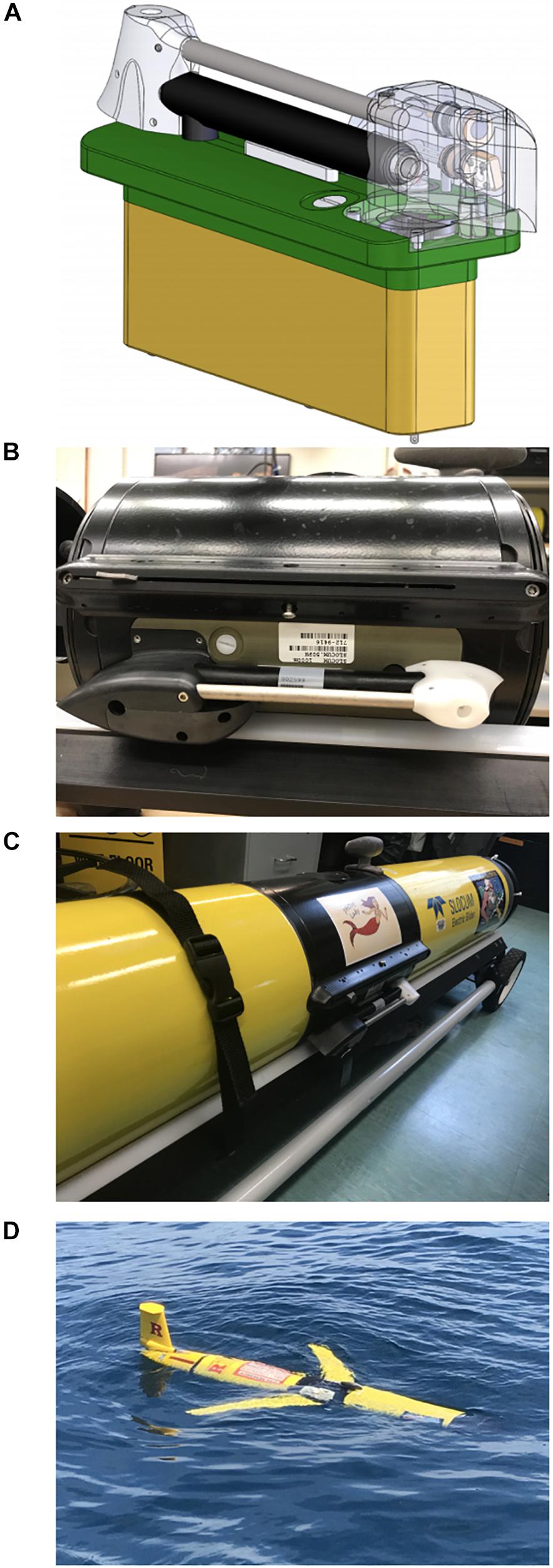
Figure 1. DeepISFET-based pH sensor integration into a glider. Deep ISFET-based pH sensor integrated with pumped CTD (A), Coupled pH and CTD integrated into a standalone science bay (B), completely assembled in the glider (C), and deployed in the Mid-Atlantic (D).

After the sensor calibrations and pre-deployment tests were completed by Sea-Bird Scientific and Teledyne Webb Research, the science sensor bay was assembled into the glider (Figure 1C) and placed in a natural seawater tank at Rutgers University for a minimum of 1 week at room temperature and pressure in order for the pH sensor to condition to seawater off the coast of Atlantic City, New Jersey (Bresnahan et al., 2014; Johnson et al., 2016).

pH Data Analysis

pH_total was calculated using the glider-measured reference voltage, pressure, sea water temperature, salinity, and sensor-specific calibration coefficients. Calculations were completed in Matlab (Johnson et al., 2017), and the code is provided in the Supplementary Material. The final equation used to calculate pH (below) was derived and modified from previous efforts (Khoo et al., 1977; Millero, 1983; Dickson et al., 2007; Martz et al., 2010; Johnson et al., 2016):

$p{H}_{total}={\displaystyle \frac{V_{ref}-k_0-k_2*t-f\left(p\right)}{S_{nernst}}}+\log \left(C{l}_T\right)+2*\log {\left(\mathrm{\gamma }HCl\right)}_{T,P}-\log (1+{\displaystyle \frac{S_T}{K_{STP}}})-\log \left({\displaystyle \frac{1000-1.005*S}{1000}}\right)$

Where:

$S_{nernst}=\frac{R*T*\text{ln}(10)}{F}$

$\log {\left(\mathrm{\gamma }HCl\right)}_{T,P}=\log {\left(\mathrm{\gamma }HCl\right)}_T+\left(\frac{V_{HC{l}^{*p}}}{\ln \left(10\right)RT}\right)/2$

R is the universal gas constant = 8.314472 J/(mol^∗K);

t is the temperature in °C;

T is the temperature in K;

S is salinity in psu;

P is the pressure in dbar;

pis the pressure in bar;

F is the Faraday constant = 96485.3415 C/mol;

k₀ is the cell standard potential offset;

k₂ is the cell standard temperature slope;

f(p)is the sensor pressure response function;

V_ref is the reference voltage;

V_HCl is the partial molar volume of HCl;

Cl_T is total chloride;

(γHCl)_T is the HCl activity coefficient at T;

(γHCl)_T,P is the HCl activity coefficient at T and p;

S_T is total sulfide;

K_STP is the acid dissociation constant of HSO_4,T&P.

Tank Tests to Determine Sensor Conditioning Time

We conducted a series of tests October 17-November 6, 2018 to determine ISFET sensor conditioning time (Figure 2A). First, the glider was placed in a tank filled with natural seawater collected from nearshore waters near Atlantic City, NJ, United States. The pH/CTD sensors were immediately turned on with data continuously recording and transmitting in real-time using a Freewave modem linked to Teledyne Webb Slocum Fleet Mission Control software. This test defined the time required of an “off the shelf” pH sensor to condition or equilibrate to local seawater. A second set of tests investigated the response of the pH sensor to various wet/dry exposure time frames, representing scenarios wherein the sensor may be kept dry for periods of a few hours to days, such as during local, overnight, or distant transit from the laboratory facility to the field prior to a deployment (Figures 2B–E). Specifically, the second set of tests determined conditioning period after: (1) the glider was turned off for 2 h while the pH sensor remained submerged in the tank, then turned back on (Figure 2B); (2) the glider was removed from the tank and the pH sensor dried for 3 h, then the glider was placed back in the tank and turned on (Figure 2C); (3) the glider was removed from the tank and the pH sensor dried for 1 day then the glider was placed back in the tank and turned on (Figure 2D); and (4) the glider was removed from the tank and the pH sensor dried for 3 days then the glider was placed back in the tank and turned on (Figure 2E). The pH sensor was considered conditioned for each set of tests after the pH measurements stabilized with minimum drift (±0.0001 pH units hour^–1 or ±0.003 pH units day^–1).

FIGURE 2

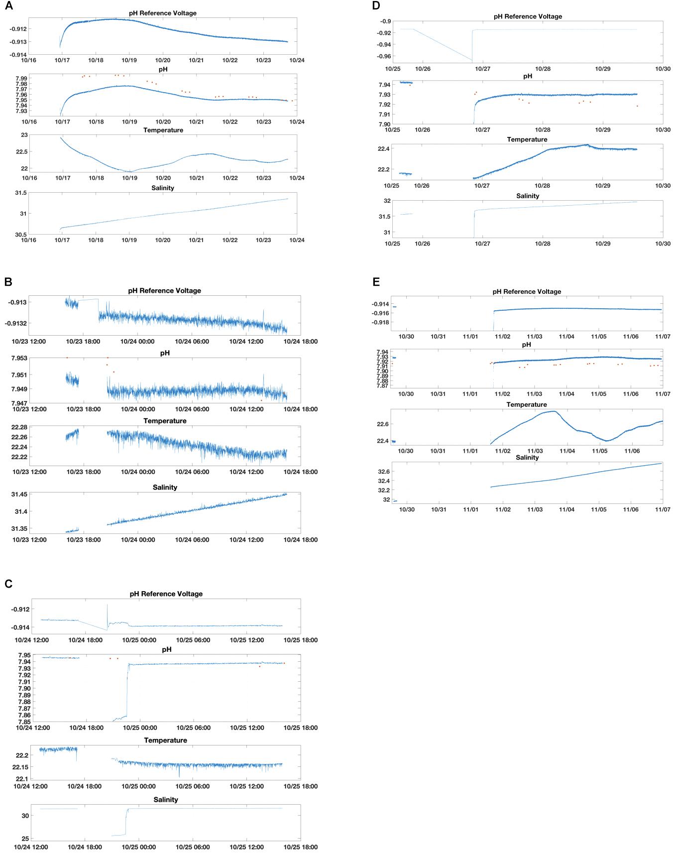
Figure 2. Glider pH and discrete (spectrophotometric) pH tank test conditioning experiments. Data shown includes pH reference voltage measurements, calculated pH, temperature and salinity over time (month/day, for longer conditioning periods; month/day time, for shorter conditioning periods). The glider was placed in a saltwater tank and the pH/CTD sensor was turned on to determine times for initial conditioning from a sensor “off the shelf” (A); conditioning after pH/CTD sensor turned off for 3 h while submerged in tank then turned back on (B); conditioning after glider removed from tank and sensor dry for 2 h then placed back in the tank and turned on (C); conditioning after glider removed from tank and sensor dry for 1 day then placed back in the tank and turned on (D); conditioning after glider removed from tank and sensor dry for 3 days then placed back in the tank and turned on (E). Data gaps represent the dry/off period.

During the tank tests, discrete seawater samples were collected from the tank next to the glider at least three times daily and measured immediately on a spectrophotometric pH system set up next to the seawater tank. Accuracy of the glider pH sensor was determined as the pH measurement offset between glider pH and pH measured spectrophotometrically after the pH glider sensor was conditioned.

First Glider Deployments

After the sensor integration, factory calibration, testing, and conditioning was complete, we tested the capability of the glider sensor package in two deployments in coastal waters along the U.S. Northeast Shelf. Slocum gliders operate by increasing and decreasing volume with a buoyancy pump to dive and climb in repeat sawtooth sampling patterns. Wings, a pitch battery, and the shape of the glider body result in forward motion with an aft rudder and internal compass maintaining a pre-programed heading while underwater. At pre-programed surface intervals the glider acquires new location information, downloads new mission parameters, and sends back real time data. The glider, RU30, used in this study was a coastal glider with a 200 m rated pump. Coastal gliders profile vertically at 10–15 cm s^–1 and travel horizontally at speeds of ∼20 km day^–1. Science sensors sample at 0.5 Hz resulting in measurements at every 20–30 cm intervals vertically.

We first deployed the glider on May 2, 2018 ∼9 km off the coast of Atlantic City, NJ (17 m water depth) (Figures 1D,3, magenta track). This glider was powered by alkaline battery pack which supports a typical deployment for 3–4 weeks. Upon deployment, we conducted a CTD hydrographic profile and several individual casts with a 5 L Niskin bottle to sample discrete seawater samples for validating the sensor (see below) while the glider was conducting dives 50–100 m from the vessel. Once water sampling was completed, the glider was sent toward its next offshore waypoint to begin its cross-shelf transect. The glider completed a full cross-shelf transect in 20 days, and was recovered on May 22, 2018 ∼24 km off the coast of Atlantic City, NJ (25 m water depth). A subset of the full glider datasets were sent to shore in near real time via Iridium satellite cell phone located in the glider tail. After each glider sampling segment the glider surfaces, inflates an air bladder in the tail section, and connects to shore via iridium satellite cell phone. These datasets included all science variables necessary to calculate pH. This allowed for initial data quality checks while the glider was deployed, and ensured that if the glider was lost critical science data was still collected. After the glider was recovered, the full datasets were downloaded from the science memory cards stored onboard and are the datasets used throughout this publication. We have made the glider variable data available and openly accessible on the ERDDAP server. The delayed mode time-series that contains all of the data as present in the source data files is accessible at: http://slocum-data.marine.rutgers.edu/erddap/tabledap/ru30-20180502T1355-trajectory-raw-delayed.html. The raw profile dataset that contains the data but broken up by glider profiles (not a time-series) is accessible at: http://slocum-data.marine.rutgers.edu/erddap/tabledap/ru30-20 180502T1355-profile-raw-delayed.html. The science dataset that contains only scientifically relevant variables is accessible at: http://slocum-data.marine.rutgers.edu/erddap/tabledap/ru30-20180502T1355-profile-sci-delayed.html. Glider data processing, including analyses for sensor time lag corrections (below), was conducted using Slocum Power Tools available at: https://github.com/kerfoot/spt.

FIGURE 3

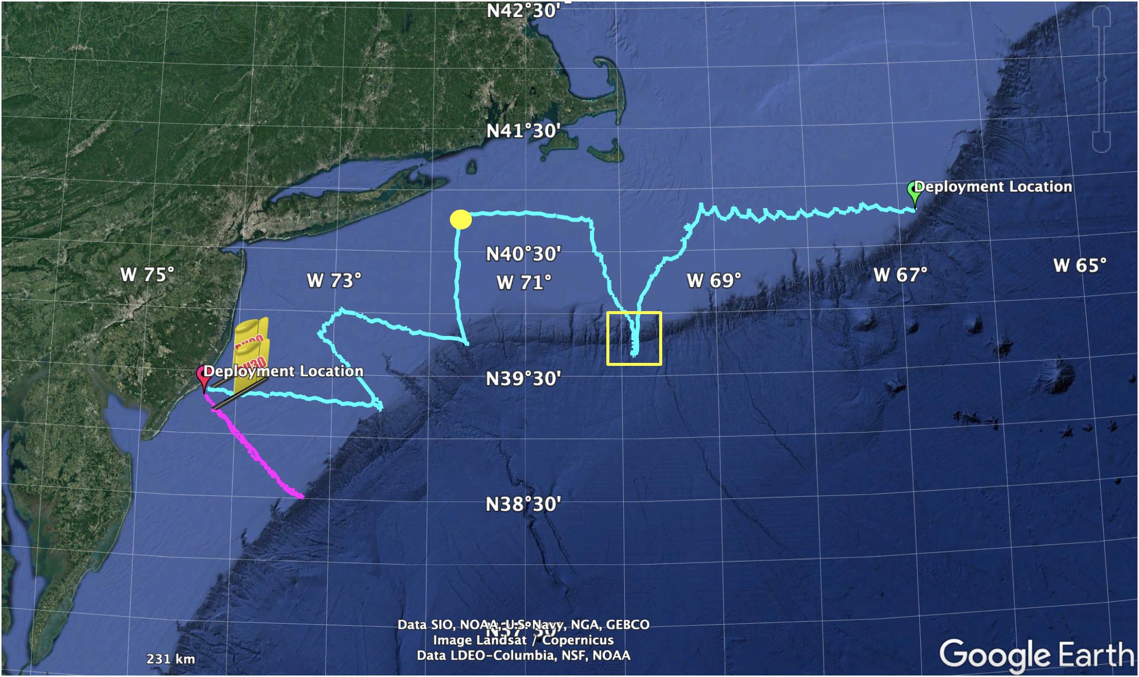
Figure 3. Map showing location of first pH glider deployments. For the first deployment (magenta track), the glider was deployed off the coast of Atlantic City, New Jersey on May 2, 2018 and took measurements of pH and other variables from nearshore to the continental shelf break and back where it was recovered on May 22, 2018. For the second deployment (cyan track), the glider was deployed east of Georges Bank on July 5, 2018 and took measurements of pH and other variables during its transit until it was recovered off the coast of Atlantic City on August 28, 2018. During this deployment the glider was entrained into a warm core ring for nearly 5 days (yellow box). Concerned about biofouling due to this extended period in warm water, we intercepted the glider south of Montauk, NJ, United States on July 31, 2018 (yellow dot) to clean and re-deploy the glider and collect additional discrete water samples for sensor validation.

A second glider deployment occurred on the eastern edge of Georges Bank on July 5, 2018 (Figure 3, cyan track). This glider was powered by a lithium battery pack (configuration was 78 DD cells in a three series) which supports a typical deployment for nearly 60 days. At the time of this deployment, discrete seawater samples were collected in surface waters within 5 m from the pH/CTD glider sensor. After which the glider was sent west over Georges Bank. During a 4–5 days period (July 18–22), the glider was entrained in a warm core ring on the shelf break in waters off southern New England (Figure 3, yellow box). Concerned about biofouling due to this extended period in warm water, we intercepted the glider south of Montauk, NJ on July 31, 2018 (Figure 3, yellow dot) to clean the glider and collect additional discrete water samples for sensor validation. The glider was moderately biofouled and included biofouling inside the sensor intake (Figure 4). The glider and sensor were cleaned as much as possible by flushing with seawater and using brushes and cloth, but we were unable to remove biofouling in the far reaches of the internal sensor surfaces. The glider was re-deployed and continued on its transit where it was recovered off the coast of Atlantic City, NJ, United States on August 28, 2018. Due the evidence of biofouling during this summer deployment, we do not present here the full datasets and only report biofouling impacts on pH measurements and derived A_T.

FIGURE 4

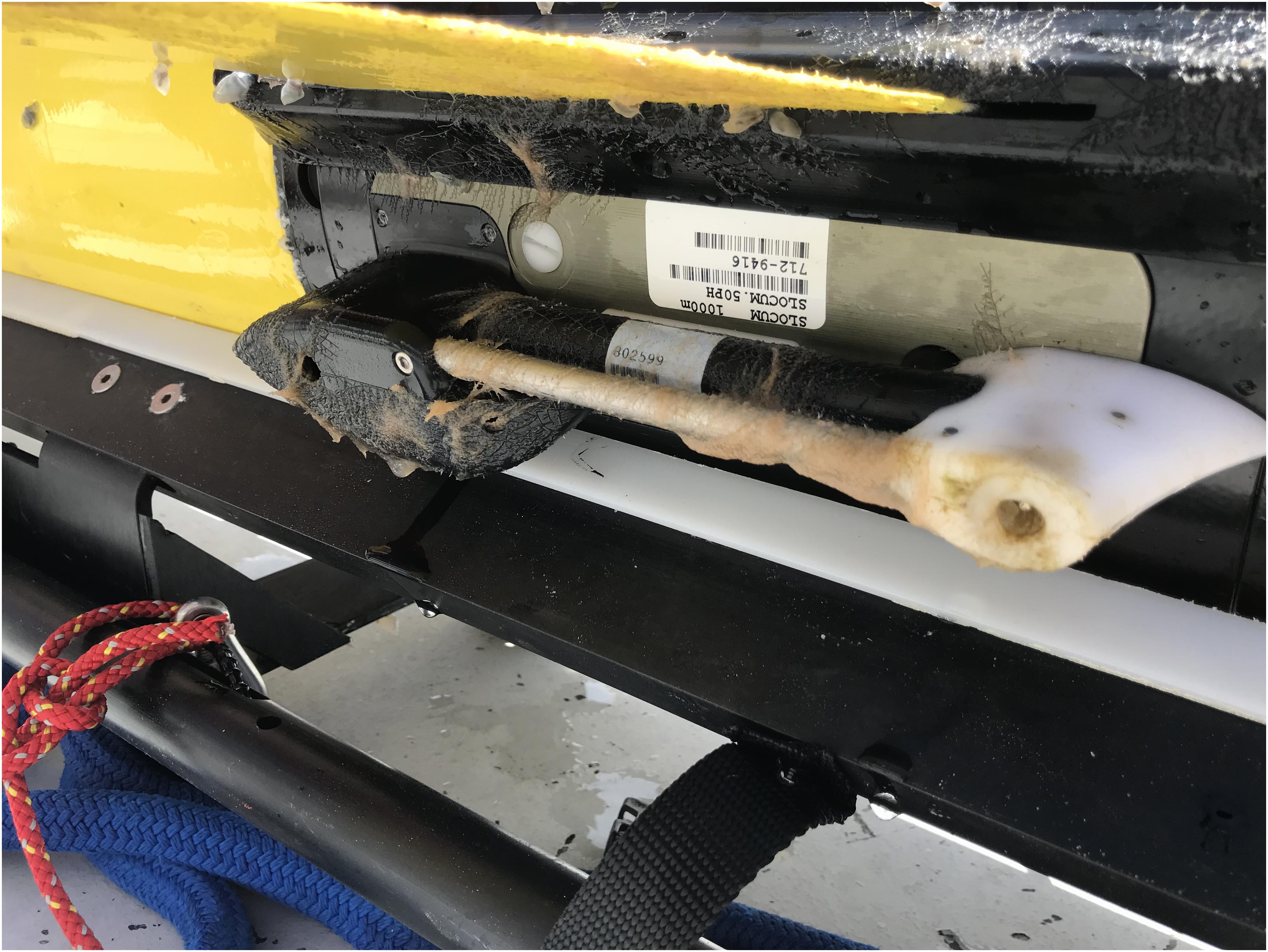
Figure 4. Biofouling on the glider deep ISFET-based pH sensor after 26 days during the July–August, 2018 deployment. The glider was intercepted, cleaned, and re-deployed south of Montauk, NJ, United States on July 31, 2018.

Sensor Time Lag Corrections

Thermal lag corrections were applied to conductivity measurements prior to calculating pH. In a standard Sea-Bird CTD temperature is measured outside of the conductivity cell while conductivity is measured inside of the cell resulting in a mismatch in the measurements then used to calculate salinity, density, and subsequently pH (Garau et al., 2011). Thermal lag typically results in incorrect salinity and density estimates when the glider profiles through sharp interfaces. To address the thermal lag, temperature and conductivity data were binned in 0.25 m increments. Sequential temperature and conductivity profile pairs (one upcast and one downcast) were averaged together and the average profile was interpolated back to the original sampling depths. Salinity was calculated based on the corrected temperature and conductivity profiles.

Reference voltage and derived pH measurements exhibited a time lag during deployment, identified as skewed shifts in upcast and downcast measured (reference electrode) and derived pH (Figures 5A,B). To correct this lag, we first identified all upcast/downcast pairs (where there is an upcast followed by a downcast during the deployment). To determine the time shift that best matches the location of the clines, in this case typically a halocline, in an upcast and subsequent downcast, each pair was run through iterations of time shifts from 0 to 120 s at 5 s intervals. Optimal time shift was identified as the shift that minimized the difference of reference voltage in the two arms of the inverse V trajectory (upcast and subsequent downcast). We plotted optimal time shift for each upcast/downcast pair over time (Figure 5C) and optimal time shifts throughout full deployment as a histogram to determine shift peaks over time (Figure 5D). We observed 2 peaks during the May 2018 deployment, so one shift (47 s) was applied to first 1/3 of the deployment and a second shift (30 s) was applied to the last 2/3 (Figures 5A,B). July had 3 peaks (46, 81, 104 s) which were applied to those corresponding sections of deployment (data not shown).

FIGURE 5

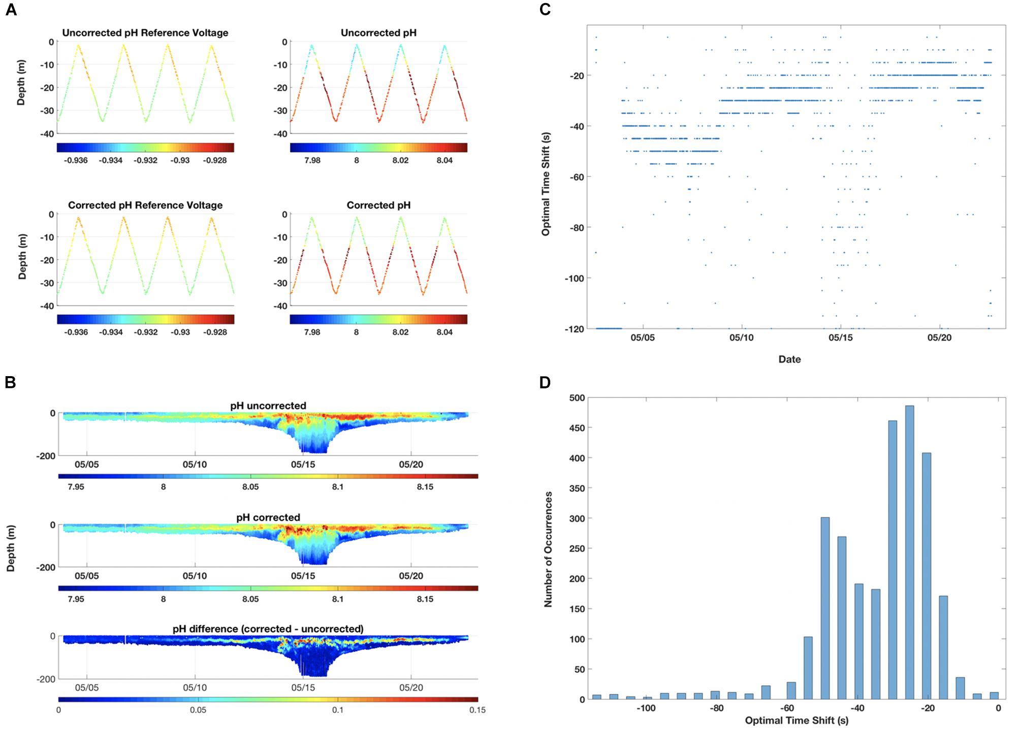
Figure 5. pH response time lag corrections. Optimal time shift was identified as the shift that minimized the difference of reference voltage in the two arms of the inverse V trajectory (upcast and subsequent downcast). Example segments of uncorrected and corrected time lag observed in glider pH reference voltage and calculated pH data during the May 2018 deployment are shown in panel (A). The time lag correction adjusted the measurements of pH reference voltage (left columns), and hence the calculations of pH (right columns). These were expanded to include uncorrected [top], corrected [middle], and the difference between the corrected and uncorrected pH [bottom] for the full May 2018 deployment (B). The optimal time shift observed for upcast and downcast pairs over time (C) and the histogram of optimal time shifts (D) during the May deployment are presented here. Peaks were applied to shift time of pH reference voltage readings in order to minimize separation between glider up and downcasts.

Total Alkalinity Estimations and Aragonite Saturation State Calculations

To complement our glider pH measurements and to fully resolve the carbonate system, A_T was estimated from simultaneous glider salinity measurements. A_T exhibits near-conservative behavior with respect to salinity in the Atlantic along the east coast of the United States (Cai et al., 2010; Wang et al., 2013). To estimate A_T, we used the following linear regression equation, determined from the salinity-A_T relationship at three cross-shelf transects along the U.S NES (Massachusetts, New Jersey, and Delaware) sampled during the ECOA-1 cruise (summer 2015) (total 170 pairs of A_T and salinity data, R² = 0.99).

$A_T={50.04}^{*}x+564.08$

Where x is salinity.

Final carbonate system parameters, including Ω_Arag, were calculated in Matlab using CO2SYS (van Heuven et al., 2011), with glider measured temperature, salinity, pressure, and pH and glider-derived salinity-based A_T as inputs. We used total pH scale (mol/kg-SW), K1 and K2 constants (Mehrbach et al., 1973) with refits (Dickson and Millero, 1987), and the acid dissociation constant of KHSO₄ in seawater (Dickson, 1990).

Quality Assurance and Quality Control (QA/QC)

The hydrographic (CTD) and DO data collected during the glider missions follows the QA/QC procedures outlined in an approved EPA Quality Assurance Project Plan (QAPP) that was developed specifically for glider observations of DO along the New Jersey coast (Kohut et al., 2014). The procedures include pre- and post- deployment steps for each sensor to ensure data quality for each deployment. Beyond these common measurements, the science bay of the glider was outfitted with an ECO puck and the profiling deep ISFET-based pH sensor. QA/QC procedures for each sensor are described in detail below.

CTD

The hydrographic data for each mission was sampled with a pumped CTD specifically engineered for this glider. Based on manufacturer specifications, the CTD was factory calibrated by SeaBird Scientific upon completion of the CTD-pH sensor integration. The QAPP requires a two-tier approach to verify the temperature and conductivity data from the glider CTD (Kohut et al., 2014). The first-tier test is a pre- and post- deployment verification between the glider CTD and a factory calibrated Sea-Bird-19 CTD in our ballast tank at Rutgers University in New Brunswick, NJ, United States. The second-tier test is an in situ verification at both the deployment and recovery of the glider. For each deployment and recovery, we lowered a manufacturer calibrated SeaBird-19 CTD to compare to the concurrent glider profile. This second-tier test gives an in situ comparison within the hydrographic conditions of the mission.

Aanderaa Optode

The DO data was sampled with an optical sensor unit manufactured by Aanderra Instruments called an optode. Like the CTD, we deployed a glider optode that is factory calibrated at least once per year. In addition to these annual calibrations, we also completed pre- and post- deployment verifications. To do this we compared optode observations to concurrent Winkler titrations of a sample at both 0 and 100% saturation. The verification for this deployment met the QAPP requirement that all optode measurements are within 5% saturation of the results of the Winkler titrations for both the 0 and 100% saturation samples (Kohut et al., 2014).

BB2FL ECO Puck

The puck we deployed was standard factory calibration from WET Labs (recommended every 1–2 years for pucks in gliders).

Profiling Deep ISFET-Based pH Sensor

We followed Best Practices for autonomous pH measurements with the DuraFET, including the recommended rigorous calibration and ground truthing procedure (Bresnahan et al., 2014; Martz et al., 2015; Johnson et al., 2016). Using a 5 L Niskin bottle aboard the vessel during deployment and recovery, replicate water samples were collected near the glider from multiple depths (0.5 m, depth of thermocline, and 2 m from bottom; see Table 1). During this 1–2 h sampling procedure, the glider sampled the water column near the vessel. Water samples were collected for pH, DIC, and A_T analysis from the Niskin bottle into two 250 mL borosilicate glass bottles for a specific depth, with one bottle for DIC and A_T and another bottle for pH. Sampling involved overflow of seawater for at least one to two volumes, after which bottles were gently filled completely to avoid gas exchange with surrounding air. One mL of sample was removed to create a small headspace to allow for seawater expansion. The sample was then poisoned with 50 μL of saturated mercuric chloride, sealed with a pre-greased glass stopper and rubber band, and stored in a cool, dark location until analysis at Cai’s laboratory (University of Delaware). Discrete sample pH was measured spectrophotometrically at 25° Celsius on the total pH scale using purified M-Cresol Purple purchased from R. Byrne at the University of South Florida (Clayton and Byrne, 1993; Liu et al., 2011). Cai’s lab has built a spec-pH unit similar to the Dickson Lab (Carter et al., 2013). The accuracy of pH data was verified against Tris buffers (Millero, 1986; DelValls and Dickson, 1998) purchased from Andrew Dickson at UCSD Scripps Institute of Oceanography and through joining inter-laboratory comparisons. A_T titrations were performed using open cell Gran titration and Apollo Scitech A_T titrator AS-ALK2 following previously described methods (Cai et al., 2010; Huang et al., 2012; Chen et al., 2015). DIC was measured using an Apollo Scitech DIC analyzer AS-C3, which acidifies a small volume of seawater (1.0 mL) and quantifies the released CO₂ with a LI-7000 Non-Dispersive InfraRed analyzer (Huang et al., 2012; Chen et al., 2015). Precision of A_T and DIC are better than ±0.1%. Measurements of A_T and DIC were quality controlled using CRMs obtained from Andrew Dickson at UCSD Scripps Institute of Oceanography. The internal consistency was first evaluated among DIC, A_T, and pH using the Excel version of CO2SYS (Pierrot et al., 2006). Then we conducted temperature correction for the measured pH values to the in situ conditions using the same Excel version of CO2SYS the guidelines for input (analysis) and output (in situ) temperature, a total pH scale (mol/kg-SW), K₁ and K₂ constants (Mehrbach et al., 1973) with refits (Dickson and Millero, 1987), and the acidity constant of KHSO₄ in seawater (Dickson, 1990). These discrete samples were compared to the glider deep ISFET pH measurements. Discrete pH and A_T measurements collected during this work are available below and in the Supplementary Material. Final carbonate system parameters on the discrete water samples were calculated using CO2SYS (Pierrot et al., 2006).

TABLE 1

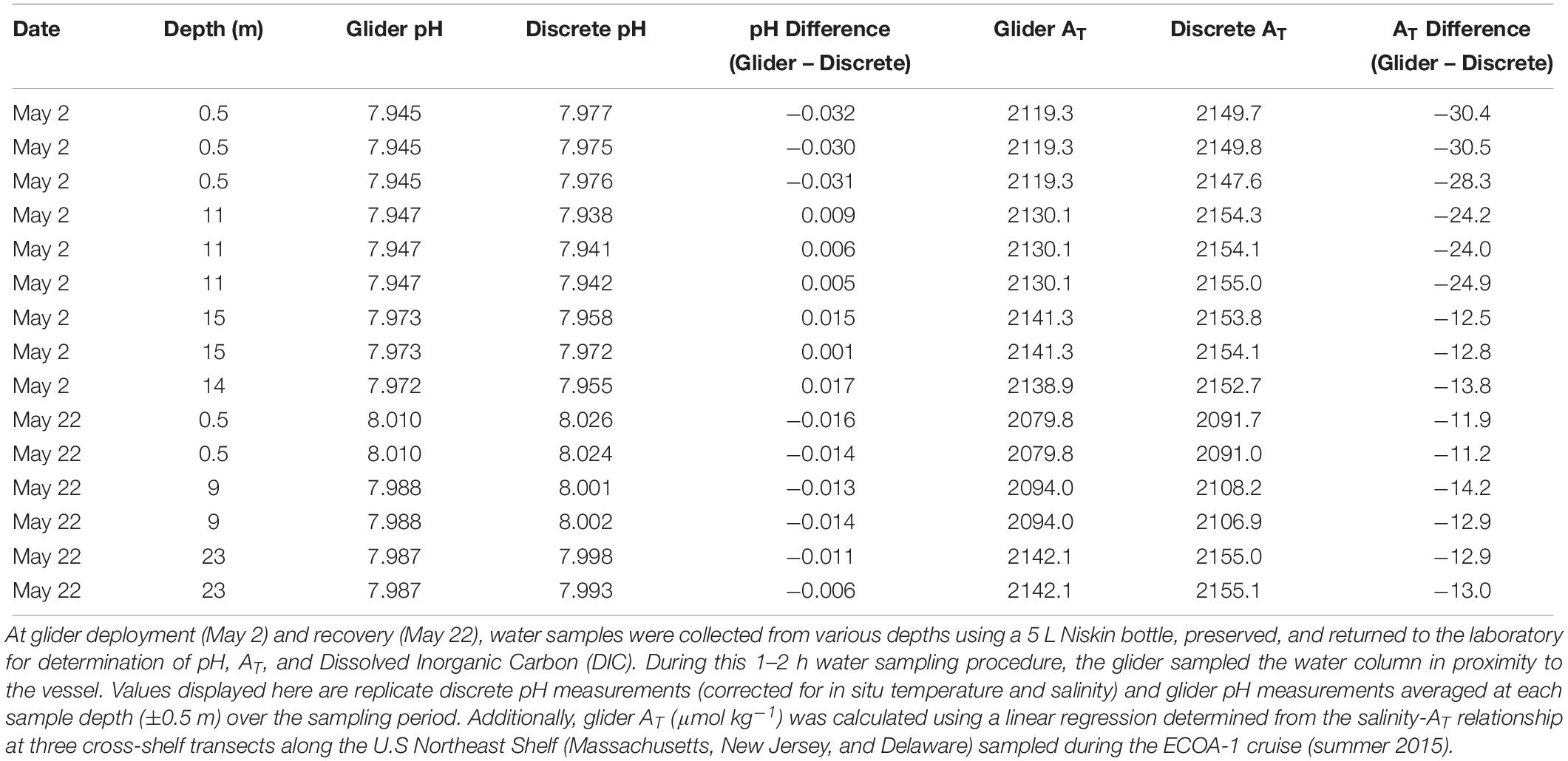
Table 1. Comparisons between glider pH and derived total alkalinity (A_T) and discrete pH and A_T measured from seawater samples during the spring glider deployment (May 2018).

Results and Discussion

Sensor Conditioning Time and Performance

Two processes occur when the Deep-Sea pH sensor is introduced to a new sample of seawater. First, the external electrode equilibrates with the new ionic concentration of the seawater or conditioning. This conditioning can take minutes to days depending on how different the ionic composition of the seawater is from the seawater the pH sensor was calibrated in at Sea-Bird (Pacific seawater collected near Hawaii). Second, the ISFET and counter electrode polarize. This polarization can take minutes to hours to complete. Once the conditioning of the pH sensor is complete, if sensor power is removed or the connection between the ISFET and the counter electrode is broken (e.g., a drying period) the sensor will need to repolarize again. We conducted a series of tests to determine sensor conditioning time initially (Figure 2A), and conditioning after variable time periods when the sensor was either turned off and kept wet or removed from tank and kept dry (Figures 2B–E). In the initial test, pH determined from the new sensor conditioned and reached within 0.005 pH units from the discrete pH values after 4–5 days of soak time in the natural seawater tank (Figure 2A and Supplementary Material). This is most likely due to the sensor equilibrating to the new seawater for the first time.

After this initial conditioning time, the pH/CTD sensor was turned off for 2 h while submerged in the tank then turned back on with the pH measurements stabilizing immediately and the offset between glider and discrete pH returning to within 0.003 pH units (Figure 2B and Supplementary Material). The glider and sensor were then turned off and removed from tank and kept dry for 3 h then placed back in the tank and turned on. The pH measurements stabilized and the offset returned to within 0.002 pH units within 17 h, and this likely occurred much sooner but discrete samples were not collected during the overnight period to confirm (Figure 2C and Supplementary Material). This conditioning was likely due to either a bubble trapped on the sensor that was cleared shortly after it was turned back on or the sensor repolarizing after being dried. The glider and sensor were then turned off and removed from tank and kept dry for 24 h then placed back in the tank and turned on. The pH sensor conditioned within 17 h, but the pH offset stabilized (±0.003 pH units) between 0.006 and 0.008 pH units for the next few days (Figure 2D and Supplementary Material). This test was repeated, except the dry period lasted 3 days prior to placing the glider/sensor back in the tank. The pH offsets stabilized (±0.003 pH units) after nearly 3 days, but this final offset between glider and discrete pH measurements was larger (0.012 – 0.015 pH units) (Figure 2E and Supplementary Material).

It is likely that after the 4–5 days of initial sensor stabilization, the sensor continued to condition or drift but at slower, gradual rate until reaching an average pH offset from discrete samples of 0.013 ± 0.001 after 18 days. This pH offset was similar to that seen in situ after initial sensor conditioning during the 3-week May 2018 glider deployment in the Mid-Atlantic Bight (absolute value range: 0.001–0.017; mean ± SD: 0.011 ± 0.005, n = 12). Therefore prior to a glider deployment, we recommend a minimum of 5 days of soak time in natural seawater collected from the field location. Another possibility for the gradual increase in pH offset between the glider and the discrete samples could be biofouling in the tank. The tank was filled with coarsely filtered, unsterilized natural seawater and kept at room temperature (not temperature-controlled). Although it was not visibly apparent, it is possible that a biofilm layer could have developed during the 18-day trial and contributed to or primarily caused the gradual sensor drift.

Nonetheless, an accuracy of 0.013 pH units achieved in the tank test (and 0.011 pH units in the field; see below) exceeded our expectations given the current specifications for this deep ISFET-based pH sensor are ±0.05 pH units in accuracy and ±0.001 pH units in precision.

In situ Glider and Discrete Sample pH and A_T Comparisons

On the first deployment (May 2018), absolute pH differences observed between glider pH and pH measured spectrophotometrically from discrete samples were quite variable, ranging from 0.001 to 0.032 pH units (Table 1). Discrepancies in the surface water at deployment were largest (mean ± SD: 0.031 ± 0.001, n = 3) compared to surface water at recovery and subsurface water at both deployment and recovery (absolute value range: 0.001–0.017; mean ± SD: 0.011 ± 0.005, n = 12). We attribute the large pH discrepancies in the surface at the start of the deployment and water sample collection to the sensor not yet being stabilized or conditioned after being out of the tank for 4–5 h during transit from the lab to the field. Offsets observed in surface water at recovery and subsurface water at both deployment and recovery might represent the logistical challenges faced when attempting to collect discrete water samples next to the glider, resulting in either salinity inputs, depth, and/or sampling time differences between glider pH measurement and pH in discrete seawater samples.

The Niskin sampling bottle used for seawater collection did not have a CTD attached which posed two challenges. First, to calculate pH using the spectrophotometric method, temperature and salinity data at target depths from the initial CTD cast conducted prior to Niskin water bottle sampling commenced were used as inputs to calculate pH. Therefore, potential salinity (and pH) changes at target depths between the CTD cast and water sampling (0.5 – 1.5 h) could have occurred due to boat drift and/or currents. Second, cable metered markings were relied upon to reach target depths, and currents or slack on the cable could have resulted in sampling at depths above the target causing mismatch between glider pH and spec pH measurements. This is supported also by high variability observed in discrete pH between replicate Niskin casts/bottle samples at certain depths (May 2, 15 m: discrepancy of 0.014 pH units; Table 1). Improvements in sampling techniques are now being employed. For example, upon deployment on July 2, surface seawater samples were collected using a Niskin water bottle deployed adjacent to the glider just after its deployment from the vessel (within a 5 m distance from the glider pH sensor), which greatly reduced the discrepancies between glider pH and discrete pH seen in the first deployment (range: 0.001–0.004 pH units; Table 2). Further improvements in water sampling technique could be made, specifically for subsurface seawater pH comparison, by using a CTD mounted on a rosette frame with multiple Niskin bottles to ensure sampling occurs at target depth and simultaneous measurements of salinity and temperature with each depth-specific sample collection.

TABLE 2

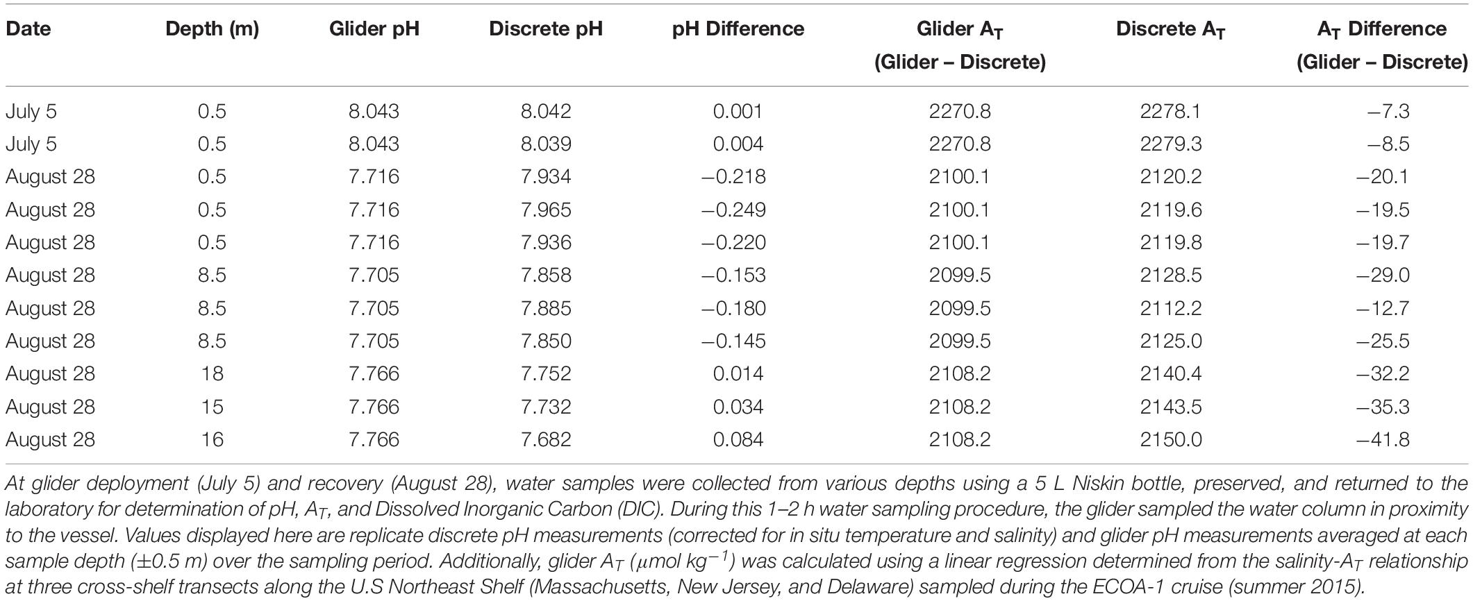
Table 2. Comparisons between glider pH and derived total alkalinity (A_T) and discrete pH and A_T measured from seawater samples during the summer glider deployment (July/August 2018).

The greatest challenge with in situ sensor validation was obtaining subsurface water samples next to the glider. During the time water sampling was being conducted on board (1–2 h), the pH glider conducted repetitive dives to sample the full water column near the vessel. While water sampling was conducted in proximity to the glider (within ∼100 m), it could have occurred far enough away that different patches were sampled by the two methods creating the offset in pH measurements. Simply, the two different sampling techniques were not measuring pH (glider) or collecting seawater for pH measurements (Niskin/discrete) at the same depths at the same place and at the same time. Future missions should test different sampling techniques (e.g., attaching glider to CTD rosette) to improve subsurface sensor validation that will minimize discrepancies at depth.

During multiple deployment and recovery practices in the U.S NES, glider salinity-based estimations of A_T were consistently lower than A_T measured in discrete samples (Tables 1–3). Overall, the differences in water column showed similar ranges of −11.2 to −30.5μmol kg^–1 for the spring deployment and recovery (Table 1) and of −7.3 to −41.8μmol kg^–1 and −6.0 to −34.8μmol kg^–1 for summer deployments and recoveries (Tables 2, 3), with averages of −18.5±7.5, −22.9±11.1, and −26.5±10.9 μmol kg^–1, respectively. The discrepancies between glider salinity-based estimates and discrete A_T likely reflect differences in water properties and/or water masses measured during these glider deployments and the summer 2015 ECOA-1 cruise (where/when the salinity-A_T relationship was derived). These include seasonal differences in low-salinity end-member and nearshore organic alkalinity input, and ultimately, challenges for sampling and validation in this dynamic environment. The offsets between glider-derived and discrete A_T yielded lower glider-estimated Ω_Arag, offset from discrete Ω_Arag by −0.010 to −0.025 for surface waters during the Spring deployment (see Supplementary Material). Further work is needed for better evaluation of the relationship between A_T and salinity at nearshore lower salinity waters and different water masses in order to reduce the uncertainty that is propogated in the calculations of Ω_Arag using CO2SYS.

TABLE 3

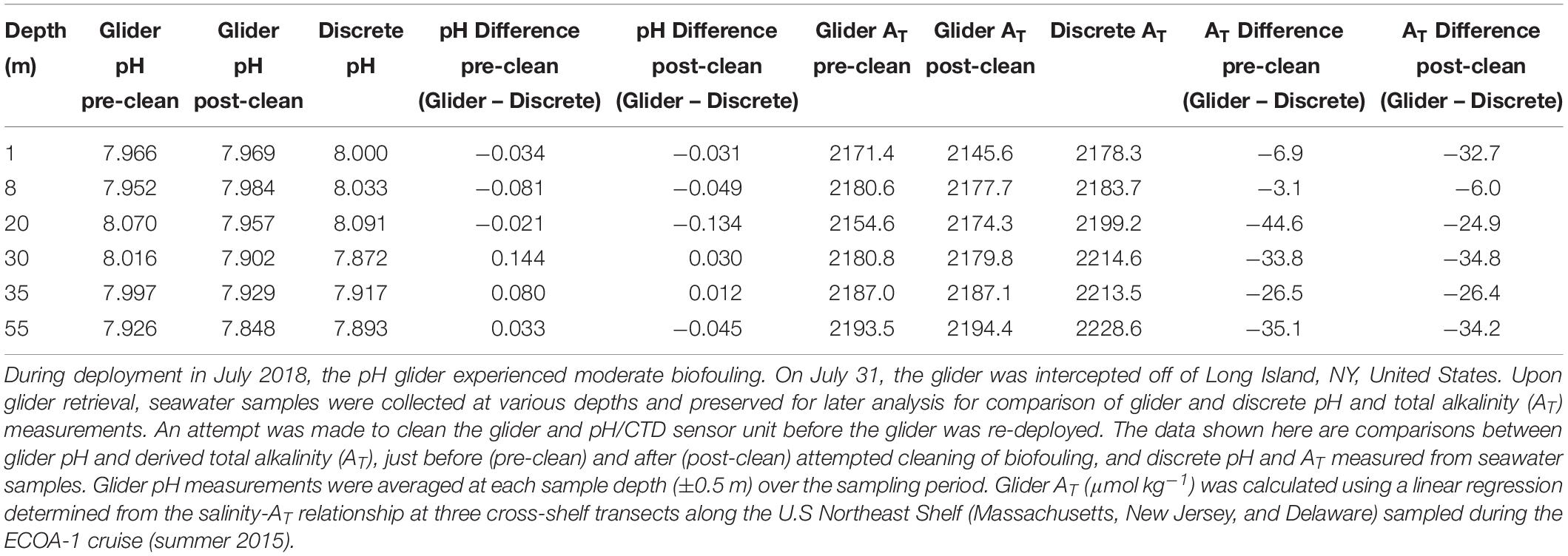
Table 3. Biofouling impacts on glider pH measurements.

Sensor Time Lags

Two patterns emerged from the pH sensor time lag correction analyses. First, there was a change in time lag throughout the deployment in May 2018 (47 s during first week, 30 s for last 2 weeks) (Figures 5C,D). This may indicate a pH sensor conditioning period, wherein the sensor was acclimating to new seawater conditions. Second, the time shift had the greatest effect in areas of abrupt water type transition, specifically in the thermocline and halocline and offshore where we encountered a warmer, saltier water mass (Figure 5B). The glider moved rapidly (10–15 cm s^–1) through these vertically narrow transition zones without acclimating completely, which possibly increased pH sensor response time and caused the increased time lag observed at these depths. This could be due to either a lag in the thermal equilibration of the sensor or salinity response of the reference electrode or relatively slow flushing of the cell by the CTD pump. Further investigations on sensor conditioning, response time, and variability are recommended in order to improve this initial lag correction method. Additionally, modifications in CTD pump flow rate or glider dive approaches in highly stratified periods in coastal systems, including slower dives or step-wise vertical descents/ascents, should be considered.

Carbonate Chemistry Dynamics in the Mid-Atlantic Bight

The pH and Ω_Arag ranges observed during this Spring (May 2018) deployment were 7.906–8.205 and 1.48–2.22 respectively. pH was frequently observed highest in subsurface waters and was associated with the depth of chlorophyll and oxygen maximums (Figure 6). Higher pH values in the chlorophyll maximum throughout the transect ranged between 7.993 and 8.127. During primary production, photosynthesis increases pH due to the uptake of CO₂. So, while the observed association between pH and chlorophyll was not surprising, the ability to resolve the subsurface pH peak from the high-resolution vertical sampling with the glider provides a valuable perspective from which to not only evaluate concurrent vertical distributions of pelagic organisms, but also to put into context past pH monitoring efforts that mostly sample surface waters (Boehme et al., 1998; Wang et al., 2013, 2017; Wanninkhof et al., 2015; Xu et al., 2017). Higher pH in offshore slope waters was also associated with a warmer, saltier water mass and suggests mixing processes could play a major role in driving pH dynamics on the shelf. During the deployment, the glider measured warmer water in the upper mixed layer on its return transect, depicting the strengthening of seasonal summer stratification in the upper mixed-layer due to incident solar radiation. These warm surface waters on the return transect were associated with increased pH values (Figure 6). Higher Ω_Arag values were consistently observed in surface waters throughout the deployment, and highest values were associated with the warm, salty, higher alkaline water mass (Figure 6).

FIGURE 6

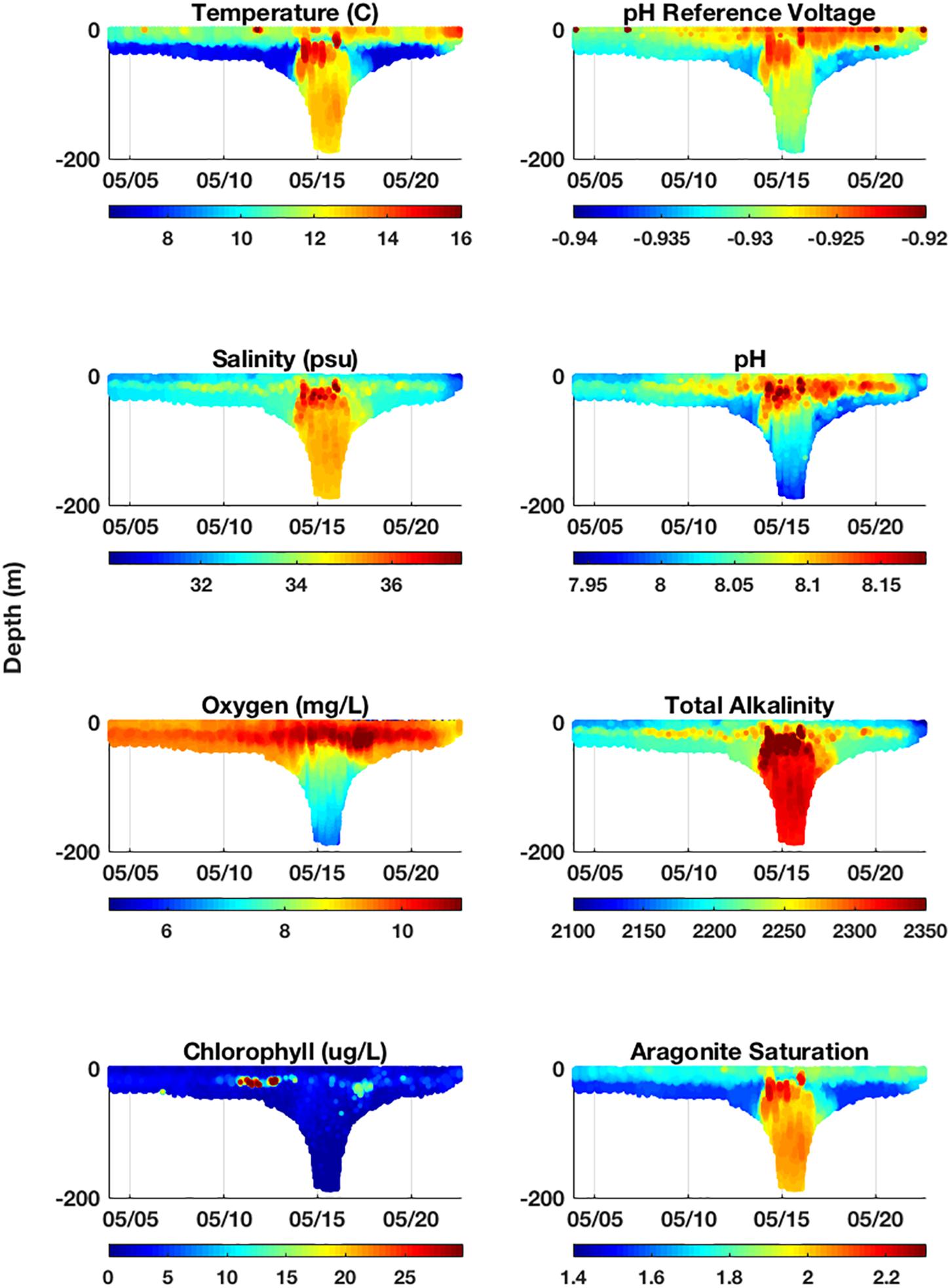
Figure 6. Complete cross-sections of variables measured by the glider and calculated from glider measurements during deployment in May 2018. The glider’s on-board scientific instruments measure temperature, conductivity (used to calculate salinity), dissolved oxygen concentration, chlorophyll fluorescence, and pH reference voltage (used to calculate pH). Salinity was used to estimate total alkalinity (TA) throughout deployment (see Methods). TA and pH were used as inputs into CO2SYS to resolve all carbonate system parameters, including aragonite saturation state, shown here.

The lowest pH typically occurred in bottom waters of the middle shelf and slope and nearshore following a period of heavy precipitation (Figure 6). Lower pH values in the mid-shelf and slope bottom waters ranged between 7.918 and 8.027. Lower pH in mid-shelf bottom water occurred in the Cold Pool as defined by remnant winter water in the Mid-Atlantic Bight centered between the 40 and 70 m isobaths (Lentz, 2017). The Cold Pool is fed by Labrador Sea slope water and is isolated when vernal warming of the surface water sets up the seasonal thermocline. The annual formation of Cold Pool water means its carbonate chemistry should reflect near real-time increases in atmospheric CO₂ and pCO₂ in its Labrador source water which is weakly buffered and exhibits lower pH and Ω_Arag (Wanninkhof et al., 2015). Thus, the dominant drivers of low pH, as well as high DIC and low Ω_Arag (Wang et al., 2013), in shelf bottom water were likely a combination of stratification, biological activity (i.e., higher respiration at depth), and the inflow of Labrador Sea slope water into the Cold Pool. Nearshore, lower pH was associated with lower salinity from freshwater input that was most substantial during a high period of precipitation near the end of the deployment, whereby 4.45 inches of rainfall was recorded at Atlantic City Marina, NJ, between May 12–22 (NJ Weather & Climate Network¹; Figure 6). This storm event resulted in the freshening of the entire water column near shore (30 m; Figure 6). River runoff has low pH from the equilibration with atmospheric CO₂ concentrations, and its zero salinity and low/zero alkalinity greatly reduces buffering capacity to offset changes in pCO₂ and contributes to low Ω_Arag (Salisbury et al., 2008; Johnson et al., 2013). Lowest Ω_Arag values consistently occurred in bottom waters on the shelf (Figure 6). This was likely driven by lower pH in these bottom waters.

When pH is plotted as a function of temperature and salinity (Figure 7), the pH characteristics of specific water masses become more apparent. For example, the fresher nearshore surface waters and surface water over the mid-shelf are distinctively different in pH (Figure 7). Thus, carbonate chemistry variability in this system over a range of scales will be driven by: (1) episodic storm mixing, upwelling, and precipitation events; (2) Mixing of water masses and the degree of horizontal intrusion of offshore water masses onto the shelf; (3) Seasonal stratification and vertical mixing/overturning processes; and (4) a combination of biological and physical drivers on the shelf and in shelf source waters. Both the horizontal and vertical gradients of pH observed were, at times, particularly sharp, and this new glider pH sensor suite demonstrated the ability to characterize the variability and drivers of this variability in these critical zones.

FIGURE 7

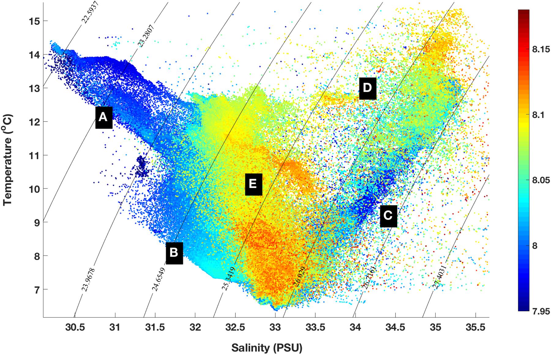
Figure 7. Temperature/Salinity plot of pH. During the May 2018 deployment, lower pH water was found in fresher nearshore surface waters (A) and bottom waters of the colder mid-shelf (B) and shelf break (C). Higher and more variable pH was found in surface water of the shelf break (D) and mid-shelf (E).

Current Limitations and Need for Future Research and Development

Comparative results between the glider deep ISFET-based pH sensor and pH measured spectrophotometrically from discrete seawater samples indicate that the glider pH sensor is capable of accuracy of 0.011 pH units or better for several weeks throughout the water column in the coastal ocean, with a precision of 0.005 pH units or better. These values are similar to those reported for the Deep-Sea DuraFET sensor deployed on moorings in Johnson et al. (2016).

However, in addition to the logistical issues related to sampling seawater next to the glider for in situ validation described above, the primary limitation we encountered and foresee is glider and sensor biofouling during deployments. Glider batteries have been evolving over time, from alkaline to lithium one-time use to rechargeable lithiums that have greatly improved the endurance capability of gliders and glider sensors. But as the potential deployment time for gliders has increased, the chance of biofouling is increased. Biofouling can impact glider flight behavior (e.g., increased drag and reduced efficiency; Rudnick, 2016) and greatly reduce sensor performance, as was observed in the SeaFET on week to month timescales (Bresnahan et al., 2014).

During our July deployment, we experienced moderate biofouling after about 3 weeks (Figure 4), which degraded the pH measurements over deployment time (Tables 2, 3). This suggests that, at a minimum, the sensor unit was impacted, yielding unreliable pH voltage data and subsequent calculations of pH. This biofouling was likely intensified when the glider was entrained in a warm core ring for a 4–5 days period. After this event, the glider was intercepted south of Montauk, NY, United States. Seawater samples collected near the glider showed the pH offsets between the glider and discrete samples were much higher compared to those at deployment (Tables 2, 3). Offsets between glider and discrete pH ranged from −0.144 to 0.081 pH units (Table 3). We made an attempt to clean the glider and sensor by flushing the sensor with seawater and using brushes of various sizes on the outer structures of the glider and sensor unit, but biofouling in the internal structure of the pH sensor unit that we could not access was still evident. Nonetheless the glider was redeployed after this cleaning process. The offsets between glider and discrete pH, ranging from −0.03 to 0.134 pH units, remained unsatisfactory (Table 3). These offsets worsened rapidly over time, and when the glider was recovered on August 28, offsets in pH measurements ranged from −0.084 to 0.249 pH units (Table 2). The magnitude and the variability of the offsets resulting from heavy biofouling yielded pH data not acceptable for OA research. The biofouling impact seems specific to the pH sensor and not the CTD, specifically the conductivity sensor. Comparisons of salinity between the glider CTD profiles and the hand-lowered SeaBird-19 CTD conducted at each glider deployment and recovery passed the in situ verification process. Furthermore, the offsets between glider derived salinity-based calculations of A_T and discrete A_T on July 31 (when the glider was intercepted and re-deployed; 24.8 ± 14.3, n = 20) and August 28 (when the glider was recovered; 26.2 ± 9.2, n = 9) were similar to those from the May deployment (18.5 ± 7.5, n = 15). It is likely that biofouling impacted pH sensor response time, as indicated by the increasing sensor time lag corrections that were applied to the glider data from the start of the deployment on July 5 to recovery on August 28 (46–81–104 s).

Current biofouling prevention measures for this sensor are the enclosure of the coupled pH/CTD sensor to block light, an anti-fouling cartridge in the pH sensor’s intake, and the active seawater pumping capability of the CTD that flushes water through the sensor package continuously during deployment. However, advances to improve anti-fouling mechanisms would greatly improve sensor performance, durability, endurance, and applicability. Approaches could include installation of an additional anti-fouling cartridge in the sensor intake and turning the glider CTD pump off at regular intervals during deployment to facilitate diffusion, concentration, and exposure of the anti-fouling agent into the water chamber surrounding the pH sensor. Furthermore, to enable sustained glider-based acidification monitoring in a coastal system, especially in warm and shallow conditions, researchers will require the ability to routinely clean and/or swap out sensors to prevent data degradation over time from biofouling.

Additionally, investigation of the mechanism that impacts pH measurements (i.e., affects on sensor response time or reference voltage readings) needs to be conducted. Finally, the current salinity-A_T relationship in the U.S. NES is only based on summer data. This relationship may be subject to change with time, particularly during other seasons, and under different conditionsthat impact freshwater influx and/or the presence of distinctive water masses in this dynamic coastal region. We recommend to determine a salinity-A_T relationship in collected water samples before and after the glider survey in order to use the salinity-based A_T together with the glider pH to reduce the uncertainty of estimating Ω_Arag.

Significance

This new glider pH sensor suite has demonstrated its potential to: (1) Provide high resolution measurements of pH in a coastal region; (2) Determine natural variability that will provide a framework to better study organism response and design more realistic experiments; and (3) Identify and monitor high-risk areas that are more prone to periods of reduced pH and/or high pH variability to enable better management of essential habitats in future, more acidic oceans. The first glider deployment reported here provided data in habitats of commercially important fisheries in the U.S. Northeast Shelf, and allowed for the examination of temporal and spatial pH variability, the identification of areas and periods of lower pH water, better understanding of how mixing events and circulation impact pH across the shelf, and the creation of a baseline to track changes over time during future, scheduled deployments. Furthermore, the integration of simultaneous measurements from multiple sensors on the glider provides the ability to not only distinguish interactions between the physics, chemistry, and biology of the ecosystem, but also to conduct salinity- and temperature-based estimates of A_T in order to derive Ω_Arag. As such, if made commercially available, this sensor suite could undoubtedly be integrated in the planned national glider network (Baltes et al., 2014; Schofield et al., 2015; Rudnick, 2016) to provide the foundation of what could become a national coastal OA monitoring network serving a wide range of users including academic and government scientists, monitoring programs including those conducted by OOI, IOOS, NOAA and EPA, water quality managers, and commercial fishing companies. Finally, data resulting from this project and future applications can help build and improve biogeochemical and ecosystem models. A range of data validated and data assimilative modeling systems has matured rapidly over the last decade in the ocean science community. Many of these systems are being configured to assimilate glider data (temperature and salinity) (i.e., ROMs). The technology produced from this project will contribute to efforts to develop coastal forecast models with the capability to predict the variability and trajectory of the low pH water.

Author Contributions

GS introduced the research ideas and led the proposal that funded this work. AB and CB developed and finalized the glider deep ISFET-based pH sensor design and provided technical support for the duration of this project. CJ worked with AB and CB on the deep ISFET-based pH sensor integration into the glider to ensure seamless hardware and software compatibility. EW-F and TM led glider data analysis efforts and figure production. BC, W-JC, and KW analyzed all discrete samples for pH, A_T, and DIC. GS wrote the draft. All authors contributed to the writing of the manuscript.

Funding

This project was funded by the National Science Foundation’s Ocean Technology and Interdisciplinary Coordination Program (NSF OCE1634520). EW-F received support from the Rutgers University Graduate School Excellence Fellowship.

Conflict of Interest

AB and CB were employed by Sea-Bird Scientific/WET Labs. CJ was employed by Teledyne Webb Research.

The remaining authors declare that the research was conducted in the absence of any commercial or financial relationships that could be construed as a potential conflict of interest.

Acknowledgments

We thank the Rutgers University Center for Ocean Observing Leadership (RU COOL) glider technicians David Aragon, Nicole Waite, and Chip Haldeman for glider preparation, deployment planning, and piloting glider missions. We also thank Rutgers undergraduate students Brandon Grosso and Laura Wiltsee for glider-based laboratory and field support, and RU COOL faculty Oscar Schofield, Josh Kohut, Scott Glenn, and Michael Crowley for facility support. We acknowledge Dave Murphy, Cristina Orrico, Vlad Simontov, and Dave Walter at Sea-Bird Scientific and Christopher DeCollibus, Clara Hulburt, and staff at Teledyne Webb Research for technical assistance. This original work was presented in October 2018 at the OCEANS’18 MTS/IEEE meeting in Charleston, SC, United States and in May 2019 at the 8th EGO meeting and International Glider Workshop in New Brunswick, NJ, United States.

Supplementary Material

The Supplementary Material for this article can be found online at: https://www.frontiersin.org/articles/10.3389/fmars.2019.00664/full#supplementary-material

Footnotes

1. ^ https://www.njweather.org/data/daily/272

References

Baltes, B., Rudnick, D., Crowley, M., Schofield, O., Lee, C., Barth, J., et al. (2014). Toward A U.S. IOOS Underwater Glider Network Plan: Part of a Comprehensive Subsurface Observing System. Silver Spring, MD: NOAA.

Google Scholar

Boehme, S. E., Sabine, C. L., and Reimers, C. E. (1998). CO2 fluxes from a coastal transect: a time series approach. Mar. Chem. 63, 49–67. doi: 10.1016/s0304-4203(98)00050-4

CrossRef Full Text | Google Scholar

Bresnahan, P., Martz, T. R., Takeshita, Y., Johnson, K. S., and LaShomb, M. (2014). Best practices for autonomous measurement of seawater PH with the honeywell durafet. Methods Oceanogr. 9, 44–60. doi: 10.1016/j.mio.2014.08.003

CrossRef Full Text | Google Scholar

Byrne, R. H., Mecking, S., Feely, R. A., and Liu, X. (2010). Direct observations of basin-wide acidification of the North Pacific Ocean. Geophys. Res. Lett. 37:L02601.

Google Scholar

Cai, W.-J., Hu, X., Huang, W.-J., Jiang, L.-Q., Wang, Y., Peng, T.-H., et al. (2010). Alkalinity distribution in the western North Atlantic Ocean margins. J. Geophys. Res. 115:C08014.

Google Scholar

Cai, W.-J., Hu, X., Huang, W.-J., Murrell, M. C., Lehrter, J. C., Lohrenz, S. E., et al. (2011). Acidification of subsurface coastal waters enhanced by eutrophication. Nat. Geosci. 4, 766–770. doi: 10.1021/es300626f

PubMed Abstract | CrossRef Full Text | Google Scholar

Carter, B. R., Radich, J. A., Doyle, H. L., and Dickson, A. G. (2013). An automated system for spectrophotometric seawater pH measurements. Limnol. Oceanogr. Methods 11, 16–27. doi: 10.4319/lom.2013.11.16

CrossRef Full Text | Google Scholar

Chen, B., Cai, W.-J., and Chen, L. (2015). The marine carbonate system of the Arctic Ocean: assessment of internal consistency and sampling considerations, summer 2010. Mar. Chem. 176, 174–188. doi: 10.1016/j.marchem.2015.09.007

CrossRef Full Text | Google Scholar

Clayton, T. D., and Byrne, R. H. (1993). Spectrophotometric seawater pH measurements: total hydrogen ion concentration scale calibration of m-cresol purple and at-sea results. Deep Sea Res. I 40, 2115–2129. doi: 10.1016/0967-0637(93)90048-8

CrossRef Full Text | Google Scholar

Cooley, S. R., Kite-Powell, H. L., and Doney, S. C. (2009). Ocean acidification’s potential to alter global marine ecosystem services. Oceanography 22, 172–181. doi: 10.5670/oceanog.2009.106

CrossRef Full Text | Google Scholar

DelValls, T. A., and Dickson, A. G. (1998). The pH of buffers based on 2-amino-2-hydroxymethyl-1,3-propanediol (‘tris’) in synthetic sea water. Deep Sea Res. Part I 45, 1541–1554. doi: 10.1016/s0967-0637(98)00019-3

CrossRef Full Text | Google Scholar

Dickson, A. G. (1990). Standard potential of the reaction AgCl(s) +0.5H2(g) = Ag(s) + HCl(aq) and the standard acidity constant of the ion HSO4– in synthetic sea water from 273.15 to 318.15 K. J. Chem. Thermodynam. 22, 113–127. doi: 10.1016/0021-9614(90)90074-z

CrossRef Full Text | Google Scholar

Dickson, A. G., and Millero, F. J. (1987). A comparison of the equilibrium constants for the dissociation of carbonic acid in seawater media. Deep Sea Res. Part A 34, 1733–1743. doi: 10.1016/0198-0149(87)90021-5

CrossRef Full Text | Google Scholar

Dickson, A. G., Sabine, C. L., and Christian, J. R. (2007). Guide to best practices for ocean CO2 measurements. PICES Spec. Publ. 3:191.

Google Scholar

Doney, S. C. (2010). The growing human footprint on coastal and open-ocean biogeochemistry. Science 328, 1512–1516. doi: 10.1126/science.1185198

PubMed Abstract | CrossRef Full Text | Google Scholar

Dore, J. E., Lukas, R., Sadler, D. W., Church, M. J., and Karl, D. M. (2009). Physical and biogeochemical modulation of ocean acidification in the central North Pacific. Proc. Natl. Acad. Sci. U.S.A. 106, 12235–12240. doi: 10.1073/pnas.0906044106

PubMed Abstract | CrossRef Full Text | Google Scholar

Feely, R. A., Alin, S. R., Newton, J., Sabine, C., Warner, M., Devol, A., et al. (2010a). The combined effects of ocean acidification, mixing, and respiration on pH and carbonate saturation in an urbanized estuary. Estuar. Coast Shelf Sci. 88, 442–449. doi: 10.1016/j.ecss.2010.05.004

CrossRef Full Text | Google Scholar

Feely, R. A., Fabry, V. J., Dickson, A. G., Gattuso, J.-P., Bijma, J., Riebesell, U., et al. (2010b). “An international observational network for ocean acidification,” in Proceedings of OceanObs’09: Sustained Ocean Observations and Information for Society, eds J. Hall, D. E. Harrison, and D. Stammer (Auckland: ESA Publication).

Google Scholar

Feely, R. A., Sabine, C. L., Hernandez-Ayon, J. M., Ianson, D., and Hales, B. (2008). Evidence for upwelling of corrosive ‘acidified’ water onto the continental shelf. Science 320, 1490–1492. doi: 10.1126/science.1155676

PubMed Abstract | CrossRef Full Text | Google Scholar

Garau, B., Ruiz, S., Zhang, W. G., Pascual, A., Heslop, E., Kerfoot, J., et al. (2011). Thermal lag correction on slocum CTD glider data. J. Atmos. Ocean. Technol. 28, 1065–1071. doi: 10.1175/JTECH-D-10-05030.1

CrossRef Full Text | Google Scholar

Hales, B., Takahashi, T., and Bandstra, L. (2005). Atmospheric CO2 uptake by a coastal upwelling system. Glob. Biogeochem. Cycles 19:GB1009.

Google Scholar

Hofmann, G. E., Smith, J. E., Johnson, K. S., Send, U., Levin, L. A., Micheli, F., et al. (2011). High-frequency dynamics of ocean pH: a multi-ecosystem comparison. PLoS One 6:e28983. doi: 10.1371/journal.pone.0028983

PubMed Abstract | CrossRef Full Text | Google Scholar

Huang, W.-J., Wang, Y., and Cai, W.-J. (2012). Assessment of sample storage techniques for total alkalinity and dissolved inorganic carbon in seawater. Limnol. Oceanogr. Methods 10, 711–717. doi: 10.4319/lom.2012.10.711

CrossRef Full Text | Google Scholar

Jiang, L.-Q., Cai, W.-J., Wang, Y., Wanninkhof, R., and Lüger, H. (2008). Air-sea CO2 fluxes on the U.S. South Atlantic bight: spatial and seasonal variability. J. Geophys. Res. 113:C07019. doi: 10.1029/2007JC004366

CrossRef Full Text | Google Scholar

Johnson, K. S. (2010). Simultaneous measurements of nitrate, oxygen, and carbon dioxide on oceanographic moorings: observing the redfield ratio in real time. Limnol. Oceanogr. 55, 615–627. doi: 10.4319/lo.2010.55.2.0615

CrossRef Full Text | Google Scholar

Johnson, K. S., Berelson, W. M., Boss, E. S., Chase, Z., Claustre, H., Emerson, S. R., et al. (2009). Observing biogeochemical cycles at global scales with profiling floats and gliders: prospects for a global array. Oceanography 22, 216–225. doi: 10.5670/oceanog.2009.81

CrossRef Full Text | Google Scholar

Johnson, K. S., Jannasch, H. W., Coletti, L. J., Elrod, V. A., Martz, T. R., Takeshita, Y., et al. (2016). Deep-Sea DuraFET: a pressure tolerant pH sensor designed for global sensor networks. Anal. Chem. 88, 3249–3256. doi: 10.1021/acs.analchem.5b04653

PubMed Abstract | CrossRef Full Text | Google Scholar

Johnson, K. S., Plant, J. N., and Maurer, T. L. (2017). Processing BGC-Argo pH Data at the DAC Level. Plouzané: Ifremer.

Google Scholar

Johnson, Z. I., Wheeler, B. J., Blinebry, S. K., Carlson, C. M., Ward, C. S., and Hunt, D. E. (2013). Dramatic variability of the carbonate system at a temperate coastal ocean site (Beaufort, North Carolina, USA) is regulated by physical and biogeochemical processes on multiple timescales. PLoS One 8:e85117. doi: 10.1371/journal.pone.0085117

PubMed Abstract | CrossRef Full Text | Google Scholar

Khoo, K. H., Ramette, R. W., Culberson, C. H., and Bates, R. G. (1977). Determination of hydrogen ion concentrations in seawater from 5 to 40 degree C: standard potentials at salinities from 20 to 45%. Anal. Chem. 49, 29–34. doi: 10.1021/ac50009a016

CrossRef Full Text | Google Scholar

Kohut, J., Haldeman, C., and Kerfoot, J. (2014). “Monitoring dissolved oxygen in new jersey coastal waters using autonomous gliders,” in Proceedings of the U.S. Environmental Protection Agency, Washington, DC.

Google Scholar

Lee, K., Tong, L. T., Millero, F. J., Sabine, C. L., Dickson, A. G., Goyet, C., et al. (2006). Global relationships of total alkalinity with salinity and temperature in surface waters of the world’s oceans. Geophys. Res. Lett. 33:L19605.

Google Scholar

Lentz, S. J. (2017). Seasonal warming of the middle atlantic bight cold pool. J. Geophys. Res. Oceans 122, 941–954. doi: 10.1002/2016jc012201

CrossRef Full Text | Google Scholar

Liu, X., Patsavas, M. C., and Byrne, R. H. (2011). Purification and characterization of meta-cresol purple for spectrophotometric seawater pH measurements. Environ. Sci. Technol. 45, 4862–4868. doi: 10.1021/es200665d

PubMed Abstract | CrossRef Full Text | Google Scholar

Martz, T., McLaughlin, K., and Weisberg, S. B. (2015). Best Practices for Autonomous Measurement of Seawater pH With the Honeywell Durafet pH Sensor. California: California Current Acidification Network (C-CAN).

Google Scholar

Martz, T. R., Connery, J. G., and Johnson, K. S. (2010). Testing the honeywell durafet^® for seawater pH applications. Limnol. Oceanogr. Methods 8, 172–184. doi: 10.4319/lom.2010.8.172

CrossRef Full Text | Google Scholar

Mehrbach, C., Culberson, C. H., Hawley, J. E., and Pytkowicz, R. M. (1973). Measurement of the apparent dissociation constants of carbonic acid in seawater at atmospheric pressure. Limnol. Oceanogr. 18, 897–907. doi: 10.4319/lo.1973.18.6.0897

CrossRef Full Text | Google Scholar

Millero, F. J. (1983). Influence of pressure on chemical processes in the sea. Chem. Oceanogr. 8, 1–88. doi: 10.1016/b978-0-12-588608-6.50007-9

CrossRef Full Text | Google Scholar

Millero, F. J. (1986). The pH of estuarine waters. Limnol. Oceanogr. 31, 839–847. doi: 10.4319/lo.1986.31.4.0839

CrossRef Full Text | Google Scholar

Pierrot, D. E., Lewis, E., and Wallace, D. W. R. (2006). MS Excel Program Developed for CO2 System Calculations Oak Ridge National Laboratory, Carbon Dioxide Information Analysis Center. Oak Ridge: US Department of Energy.

Google Scholar

Rudnick, D. L. (2016). Ocean research enabled by underwater gliders. Ann. Rev. Mar. Sci. 8, 519–541. doi: 10.1146/annurev-marine-122414-033913

PubMed Abstract | CrossRef Full Text | Google Scholar

Rudnick, D. T., Davis, R. E., Eriksen, C. C., Fratantoni, D. M., and Perry, M. J. (2004). Underwater gliders for ocean research. Mar. Technol. Soc. J. 38, 48–59.

Google Scholar

Salisbury, J., Green, M., Hunt, C., and Campbell, J. (2008). Coastal acidification by rivers: a threat to shellfish? Eos Transl. Am. Geophys. Union 89, 513–528.

Google Scholar

Schofield, O., Jones, C., Kohut, J., Kremer, U., Miles, T., Saba, G., et al. (2015). Developing Coordinated Communities of Autonomous Gliders for Sampling Coastal Ecosystems. Mar. Tech. Soc. J. 49, 9–16. doi: 10.4031/mtsj.49.3.16

CrossRef Full Text | Google Scholar

Schofield, O., Kohut, J., Aragon, D., Creed, L., Graver, J., Haldeman, C., et al. (2007). Slocum gliders: robust and ready. J. Field Robot. 24, 1–14.

Google Scholar

Seidel, M. P., DeGrandpre, M. D., and Dickson, A. G. (2008). A sensor for in situ indicator-based measurements of seawater pH. Mar. Chem. 109, 18–28. doi: 10.1016/j.marchem.2007.11.013

CrossRef Full Text | Google Scholar

Thomsen, J., Gutowska, M. A., Saphörster, J., Heinemann, A., Trübenbach, K., Fietzke, J., et al. (2010). Calcifying invertebrates succeed in a naturally CO2-rich coastal habitat but are threatened by high levels of future acidification. Biogeoscience 7, 3879–3891. doi: 10.5194/bg-7-3879-2010

CrossRef Full Text | Google Scholar

van Heuven, S., Pierrot, D., Rae, J. W. B., Lewis, E., and Wallace, D. W. R. (2011). MATLAB Program Developed for CO2 System Calculations. ORNL/CDIAC-105b. Carbon Dioxide Information Analysis Center. Oak Ridge: U.S. Department of Energy.

Google Scholar

Vandemark, D., Salisbury, J. E., Hunt, C. W., Shellito, S. M., Irish, J. D., McGillis, W. R., et al. (2011). Temporal and spatial dynamics of CO2 air-sea flux in the Gulf of Maine. J. Geophys. Res. 116:C01012.

Google Scholar

Wang, H., Hu, X., Cai, W.-J., and Sterba-Boatwright, B. (2017). Decadal fCO2 trends in global ocean margins and adjacent boundary current-influenced areas. J. Geophys. Res. 44, 8962–8970. doi: 10.1002/2017GL074724

CrossRef Full Text | Google Scholar

Wang, Z. A., Wanninkhof, R., Cai, W.-J., Byrne, R. H., Hu, X., Peng, T.-H., et al. (2013). The marine inorganic carbon system along the Gulf of Mexico and Atlantic coasts of the United States: Insights from a transregional coastal carbon study. Limnol. Oceanogr. 58, 325–342. doi: 10.4319/lo.2013.58.1.0325

CrossRef Full Text | Google Scholar

Wanninkhof, R., Barbero, L., Byrne, R., Cai, W.-J., Huang, W.-J., Zhang, J.-Z., et al. (2015). Ocean acidification along the Gulf Coast and East Coast of the USA. Cont. Shelf Res. 98, 54–71. doi: 10.1016/j.csr.2015.02.008

CrossRef Full Text | Google Scholar

Xu, Y.-Y., Cai, W.-J., Gao, Y., Wanninkhof, R., Salisbury, J., Chen, B., et al. (2017). Short-term variability of aragonite saturation state in the central Mid-Atlantic Bight. J. Geophys. Res. Oceans 122, 4274–4290. doi: 10.1002/2017JC012901

CrossRef Full Text | Google Scholar

Xue, L., Cai, W.-J., Hu, X., Sabine, C., Jones, S., Sutton, A. J., et al. (2016). Sea surface carbon dioxide at the georgia time series site (2006–2007): Air–sea flux and controlling processes. Prog. Oceanogr. 140, 14–26. doi: 10.1016/j.pocean.2015.09.008

CrossRef Full Text | Google Scholar

Yu, P. C., Matson, P. G., Martz, T. R., and Hofmann, G. E. (2011). The ocean acidification seascape and its relationship to the performance of calcifying marine invertebrates: laboratory experiments on the development of urchin larvae framed by environmentally-relevant pCO2/pH. J. Exp. Mar. Biol. Ecol. 400, 288–295. doi: 10.1016/j.jembe.2011.02.016

CrossRef Full Text | Google Scholar