Epibenthos Dynamics and Environmental Fluctuations in Two Contrasting Polar Carbonate Factories (Mosselbukta and Bjørnøy-Banken, Svalbard)

Introduction

Arctic Carbonate Factories

Biogenic carbonate production by benthic skeletal organisms on the shelf and in coastal waters of the Arctic Svalbard Archipelago supports the northernmost cold-water ‘carbonate factories’ known to date. This pithy term was coined by Schlager (2000, 2005), who recognised various types of such centres of carbonate production, including the end-members ‘T factory’ (tropical + top-of-the-water-column) and ‘C factory’ (cool water + controlled precipitate). In contrast to the extensively studied T factories, the biosedimentary dynamics of their polar counterparts is still poorly known (for reviews, see James and Clarke, 1997; Pedley and Carannante, 2006). The Svalbard C factories have evolved between Bjørnøya (Bear Island) and northern Spitsbergen upon retreat of the last glacial ice sheet during the early Holocene, despite presumably unfavourable environmental conditions characterised by cold waters with low carbonate saturation, iceberg ploughing, high aeolian and glacial terrigenous input, as well as extreme seasonality (e.g., Henrich et al., 1995, 1996, 1997; Teichert et al., 2012, 2014).

Among the most significant carbonate producers in polar C factories are calcifying crustose coralline red algae (Rhodophyta), and particularly their non-attached mobile sedimentary aggregates, called rhodoliths. They serve as ‘bioengineers’ that provide habitat for a great variety of invertebrate species (Foster, 2001; Barbera et al., 2003). In particular, Lithothamnion glaciale has a widespread distribution and contributes substantially to cold-temperate and polar carbonate production. It is the key species in the extensive Svalbard rhodolith beds (Teichert et al., 2014; Teichert and Freiwald, 2014). This includes the northernmost occurrences of this species known to date, forming rhodolith beds at more than 80° N latitude at Svalbard’s Nordkappbukta (Teichert et al., 2012). Recent findings suggest that L. glaciale is much more widespread in polar waters than previously thought and shows a high specialization and adaptive potential to extreme seasonality, and with respect to interactions with associated biota (Teichert et al., 2012, 2014). The kelp alga Laminaria latissima is another macrophyte of relevance for carbonate production, albeit by indirect means in that they provide substratum, protection and food, and by influencing the aqueous carbonate system in the water column. In contrast to the rhodolith beds, kelp forests are more prominent in the southern part of the archipelago, in particular on Spitsbergen-Banken (Suess et al., 1994; Andruleit et al., 1996; Henrich et al., 1996, 1997; Wiodarska-Kowalczuk et al., 2009). Among the invertebrate calcifiers it is mainly the large clam Chlamys islandica, the thick-shelled Mya truncata, and the bioeroding bivalve Hiatella arctica, as well as the barnacle Balanus balanus that contribute to the intense carbonate production, complemented by various species of serpulid worms, bryozoans, benthic foraminiferans, gastropods, and echinoderms (e.g., Andruleit et al., 1996; Henrich et al., 1996, 1997; Teichert et al., 2012, 2014).

It has been shown that the structural complexity of Svalbard carbonate factories – and the rhodolith beds in particular – promote a biodiversity richer than in their surrounding environment (Teichert, 2014). On a larger scale, the Barents Sea shelf counts among the most biodiverse regions in the Arctic (Piepenburg et al., 2011; CAFF, 2017), which has been proposed to be based on tight cryo-pelago-benthic coupling resulting in a high food supply supporting benthic biomass and diversity development (Grebmeier and Barry, 1991; Piepenburg, 2005). In this respect, the Svalbard area is regarded as a ‘hot spot’ and several studies consequently revealed the development of rich benthic communities (e.g., Piepenburg et al., 1996; Hop et al., 2002; Weslawski et al., 2003; Kuklinski and Barnes, 2005; Kuklinski et al., 2006). The geographical distribution of the rhodolith communities, their habitat preferences and their interaction with benthic invertebrate fauna in the Barents Sea, however, is understudied, which applies also for the prominent shell-beds and kelp forests on the Spitsbergen- and Bjørnøy-Banken.

A better understanding of the environmental setting and biosedimentary dynamics of these carbonate factories is paramount, considering the alarming impact of global change on polar environments (Barnes and Tarling, 2017). The northern hemisphere is currently experiencing a dramatic long-term sea-ice decline, which is a striking effect of the ongoing ocean warming (Kerr, 2012; Halfar et al., 2013; Hetzinger et al., 2019). Ocean warming in concert with ocean acidification (OA) is of particular relevance when studying the Holocene evolution of the polar C factories and for modelling their future development. Coralline algae, for instance, are considered to be among the first organisms to respond to ocean acidification due to their high-Mg calcite skeleton, which is the most soluble form of CaCO₃ (Morse et al., 2006; Basso, 2012; Basso and Granier, 2012). Hence, L. glaciale and other calcifiers thriving in cold waters, where the calcium carbonate ion saturation (Ω) is naturally low and lowering fastest, will find it increasingly hard to build their calcareous skeletons (Orr et al., 2005; Doney et al., 2009; Büdenbender et al., 2011; Diaz-Pulido et al., 2012; McConnico et al., 2014; Raddatz et al., 2016). In addition, it has been shown that chemical bioerosion (biocorrosion) by microendoliths and other biota involving chemical dissolution is accelerated by OA (for a review, see Schönberg et al., 2017). Calcifiers may thus suffer from the combination of compromised calcification and increasing rates of bioerosion. A decrease in coralline algae abundance could lead to an ecosystem dominated by non-calcifying species (Kuffner et al., 2007; Hall-Spencer et al., 2008), associated with a loss in microhabitat complexity and a decline in associated biodiversity.

RV Maria S. Merian Cruise 55

To better understand the habitat characteristics and biosedimentary dynamics of the Svalbard C factories, the RV Maria S. Merian expedition MSM55 (acronym ARCA), led a team of scientists of SENCKENBERG am Meer in Wilhelmshaven and GEOMAR in Kiel (both in Germany), to target two contrasting sites of intense biogenic carbonate production in the coastal waters of Svalbard (see Wisshak et al., 2017 for the cruise report). These are the rhodolith beds in Mosselbukta in the far north of the archipelago and the extensive biogenic carbonate sediments accumulating in the strong hydrodynamic regime of the Spitsbergen- and Bjørnøy-Banken south of Spitsbergen. The MSM55 research programme focussed on bathymetrical gradients from the intertidal zone to aphotic depths, following a holistic approach: The scientific disciplines and methodological tool-kit comprised hydroacoustic habitat mapping (multibeam-echosounder and sidescan-sonar), visual habitat mapping (research submersible and drop-camera), hydrographic investigations including assessment of the aqueous carbonate system (CTD and water samples), macrobenthos inventory (beam-trawls and excursions to shore), recording of short-term environmental fluctuations and benthic community dynamics (lander deployments), classical carbonate facies analysis of source and export areas (Shipek-grabs and excursions to shore), and an evaluation of carbonate (re)cycling, including budgeting calcification versus bioerosion (recovery of a 10-year settlement experiment). Complementing investigations concerned on-board acidification and temperature stress experiments with the key calcifier L. glaciale, and sampling of long-lived rhodophytes for geochemical establishment of calibrated sea-ice proxy time series. This multi-disciplinary framework of objectives and methods allows for a detailed comparison of the two contrasting types of polar carbonate factories.

In the present contribution we will focus first on the general water mass characteristics and variability of environmental parameters (density patterns, nutrient regime, carbonate system, stable isotope signature). These were assessed via data from (1) CTD profiling, (2) water sampling, (3) two short-term lander deployments, and (4) a CT data logger recovered with a 10-year settlement experiment. We will then address various aspects of the macrobenthos biodiversity and dynamics as recorded by time series of high resolution seafloor images captured by (5) the lander’s camera system. Finally, the benthos dynamics of carbonate producing and degrading key species will be set in the context of short-term environmental fluctuations.

The Study Sites

Mosselbukta (=‘shellfish bay’) is a classical site for geo-biological research on carbonate production by benthic communities in Svalbard waters and is located at the mouth of Wijdefjorden in northernmost Spitsbergen (Figure 1A). The pioneering work of Kjellman (1883) reported rhodolith beds several square kilometres in extent, drawing our attention to this location and triggering a first research cruise with RV Maria S. Merian to this site in August 2006 (MSM2-3; see Lherminier et al., 2009 for the cruise report). Based on data from this field campaign, a first characterisation of these northernmost rhodolith beds and their biological and environmental controls was undertaken by Teichert et al. (2012, 2014). Also, carbonate production rates and their relation to fluctuations in solar radiation were assessed (Teichert and Freiwald, 2014). Glaciogenic pebbles to boulders litter the seafloor in Mosselbukta, providing suitable hardground for crustose coralline algae. Lithothamnion glaciale is the dominant rhodophyte species, encountered down to a dysphotic 70 m water depth. Carbonate production appears most pronounced at around 45 m water depth, where rhodoliths of up to 25 cm in diameter cover 60–80% of the seafloor (Teichert et al., 2014). During MSM55, most of the bay was mapped from the shore down to the bottom of the fjord at about 180 m water depth (Figure 1B).

FIGURE 1

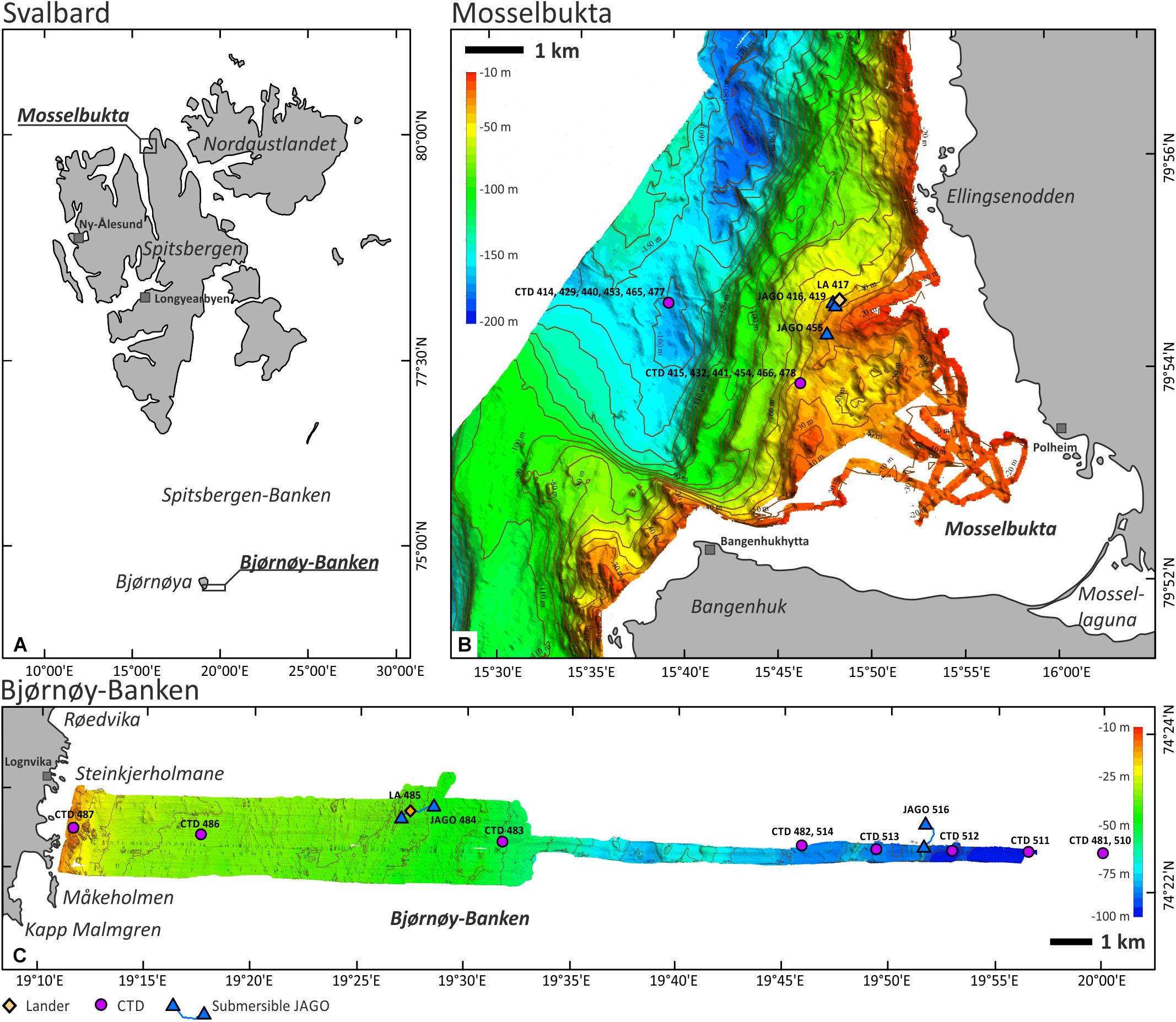
Figure 1. (A) The Svalbard Archipelago (Norwegian legislation) and the location of the two study sites. (B) Mosselbukta in the north of Spitsbergen with the MSM55 multi-beam bathymetry and the location of the relevant CTD, SaM Lander, and JAGO stations. (C) Bjørnøy-Banken in the far south of the archipelago with the MSM55 multi-beam bathymetry and the location of the relevant CTD, SaM Lander, and JAGO stations.

Spitsbergen-Banken, with Bjørnøy-Banken at its southwestern corner, is a shallow (20–150 m) shelf platform with an extent of ∼80,000 km² spanning from Bjørnøya to Hopen (Figure 1A). The bank is delineated by the continental margin to the west and the Barents and Stjorfjord Troughs to the south and north, respectively, and is deeply incised by the Kveitehola Trough. These troughs are pathways for major sediment fluxes from the Barents shelf to the continental slope fan systems, particularly during the last deglaciation. Today, upwelling warm (5–8°C) and saline Atlantic water masses reach the top of Spitsbergen-Banken along these troughs and entrap cold (<3°C) and less saline Arctic water masses that form a clockwise gyre with the boundary between the two water masses being referred to as the Oceanic Polar Front (Johannessen and Foster, 1978). Primary production during plankton blooms that form along the Polar Front during melting of the seasonal winter sea ice masses provide nutrition for a rich calcareous epibenthos community, which support the local carbonate factory within its strong hydrodynamic regime driven by storm waves and the local gyre (Henrich et al., 1997). A series of exploratory cruises with the RV Meteor in the early nineties (Gerlach and Graf, 1991; Pfannkuche et al., 1993; Suess et al., 1994) documented the existence of one of the largest Arctic carbonate platforms covered to a large extent by barnacle and bivalve shell beds forming large-scale, subaqueous carbonate sand dunes (Henrich et al., 1995, 1996, 1997, and references therein). The spatial architecture and biosedimentary dynamics of the carbonate production are still poorly known, but prominent kelp forests thriving on the shallowest hardgrounds are plausible candidates as centres of carbonate production (Henrich et al., 1996) by providing substrate for a rich calcareous epifauna on their fronds and amongst their holdfasts (Scoffin, 1988; Freiwald, 1998). In addition, shellfish banks and barnacle bioherms are found interlocked with other Holocene carbonate sediments (Wiborg, 1970). While crustose coralline algae are typical constituents of the encrusting hard-bottom communities at the southwestern flank of Spitsbergen-Banken (Henrich et al., 1997), rhodolith fields, like in northern Spitsbergen, were not documented as yet. The bathymetrical transect studied herein is located near the southern tip of Bjørnøya and extends from the shore due east across Bjørnøy-Banken to a water depth of 110 m (Figure 1C).

Materials and Methods

Settlement Platform

A complete seasonal cycle of temperature and salinity (see Table 1 for an overview of all data reported in this study), spanning August 2006 to November 2007, was logged by a Star-Oddi DST CT miniature logger that was mounted on a settlement platform recovered during MSM55 with submersible JAGO (station MSM55/455). This platform was deployed 10 years earlier at the same water depth (46 m) and in close proximity to the position of the SaM Lander in 2016 (see below). Measurements were taken in 20 min intervals with an accuracy of ±0.1°C and ±0.75 salinity points on the Practical Salinity Scale (PSS). In addition, the seawater density (σ_Θ) was calculated from temperature and salinity. Due to corrosion of the conductivity contacts, the salinity values during the second half of the data set were most likely compromised by a drift artefact, compensated by a drift correction of −0.2 on the PSS scale per month, beginning in May 2007. The logger data were set in context to the duration of the polar night and polar day at the deployment site, computed using the Planetcalc online calculator¹, and the presence of drift ice in the area, as derived from the 2006–2007 ice chart archives of the Norwegian Ice Service at the Norwegian Meteorological Institute².

TABLE 1

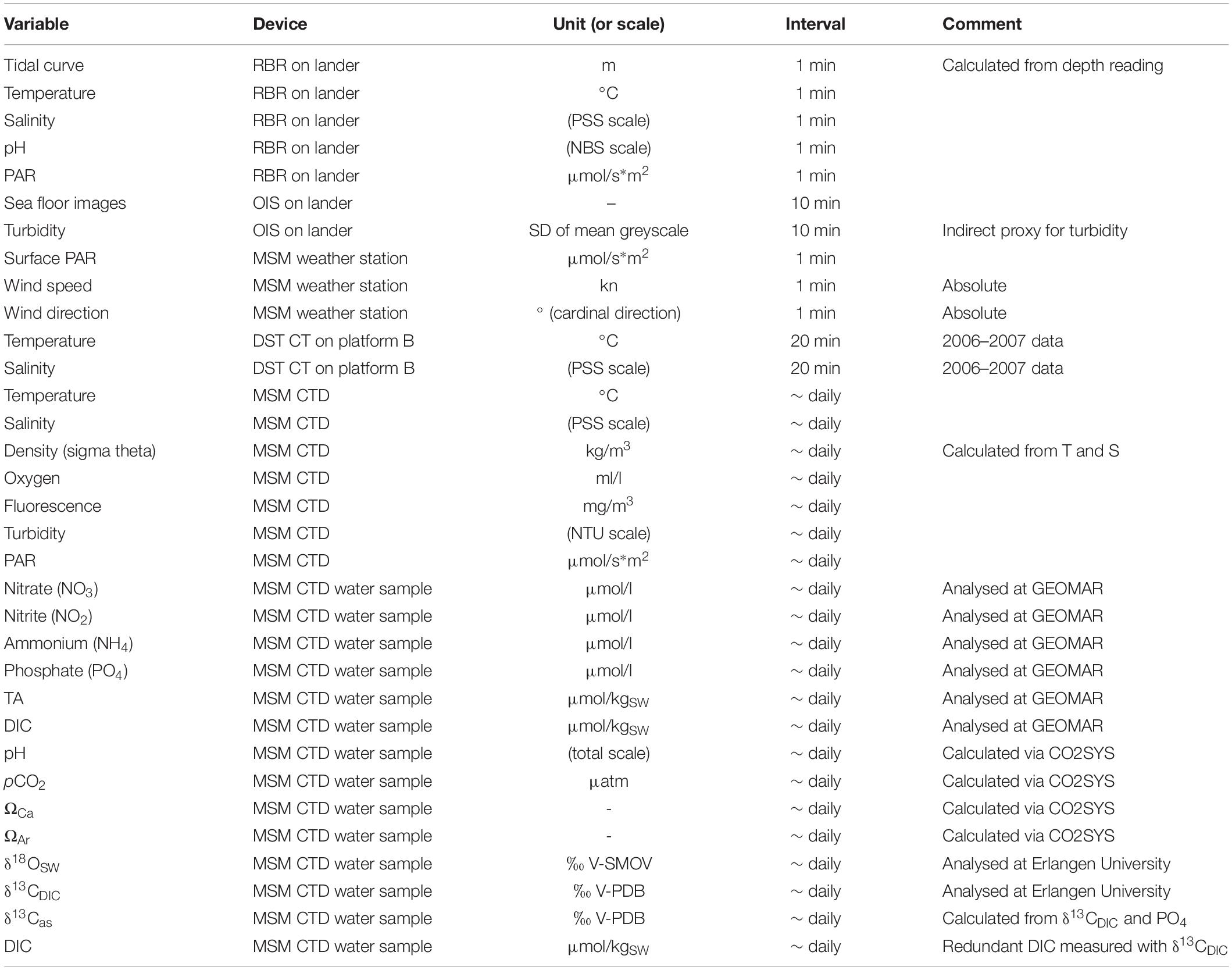
Table 1. Overview of data and environmental variables reported in this study, with specifications of the applied instruments, the unit or scale the values are reported in, and the temporal resolution.

CTD

The conductivity, temperature, depth (CTD) system employed was the shipboard Sea-Bird Electronics SBE 911plus, built into a SBE 32 rosette housing capable of holding 24 10-l water samplers (Niskin-type). For reasons of redundancy and quality control, the system was equipped with two SBE units resulting in double measurements of conductivity (Sea-Bird SBE 04C), temperature (Sea-Bird SBE 03+), pressure (Digiquartz), dissolved oxygen (Sea-Bird SBE 43), and calculated density and sound velocity. Additional sensors were attached to determine fluorescence and turbidity [WETLabs ECO FLNTU(RT)D] and photosynthetically active radiation (Biospherical QSP-2300 PAR Sensor). Accuracy (and resolution) of the various measured parameters reported by Sea-Bird (for 24 Hz sampling rate) are specified as ±0.0003 mS/cm (∼0.0004 mS/cm) for conductivity, ±0.001°C (<0.0003°C) for temperature, ±0.001% (<0.001%) for pressure, ±2% of saturation for dissolved oxygen, and about <3% (stability < 0.003 μmol/s^∗m² for dark reading) for the photosynthetically active radiation (PAR). Bottom alarm was released through a pilot weight 5 m above the seafloor and additionally controlled with a Teledyne Benthos PSA-916 altimeter. Live data was processed with the Sea-Bird software SBE Seasave (v. 7.22) and further processing was performed using SBE Data Processing (v. 7.22.0) and Ocean Data View (v. 4.7.2)³.

Water Sampling

Water samples were taken with the shipboard rosette SBE 32 and the JAGO Niskin bottle for analysis of stable oxygen and carbon isotopes (δ¹⁸O and δ¹³C_DIC), dissolved inorganic carbon (DIC) and total alkalinity (TA), as well as dissolved inorganic nutrients (nitrate, nitrite, ammonium, phosphate). Samples were taken at ∼10 m water depth and 5 m above the seafloor. Samples for stable oxygen and carbon isotopes, DIC and TA were sampled according to standard procedures (Dickson et al., 2007) and stored in glass vials, poisoned each with 50 μl HgCl₂ to arrest biological activity. The vials were sealed with aluminium caps and high density butyl-rubber-plugs. Samples for nutrient analyses were stored in 100 ml glass vials and kept frozen at −20°C until measurement.

Nutrient Analyses

The dissolved inorganic nutrients nitrate (NO₃), nitrite (NO₂), and phosphate (PO₄) were analysed with a four-channel Automated Continuous Segmented Flow Analyzer (QuAAtro39, SEAL Analytical) with detection limits of 0.03 μmol/l for NO₃, 0.01 μmol/l for NO₂, and 0.01 μmol/l for PO₄. Dissolved inorganic ammonium (NH₄) was quantified using a San++ Automated Continuous Flow Analyzer (Skalar) with a detection limit of ∼ 0.15 μmol/l. All nutrients were analysed based on the general methods described by Hansen and Koroleff (1999).

Carbonate System Analyses

DIC was measured using an Automated Infrared Inorganic Carbon Analyzer (AIRICA with LI-COR 7000, Marianda) calibrated using certified reference material for oceanic CO₂ measurements (A. G. Dickson, Scripps Institution of Oceanography, batch # 115). Each sample was measured four times by the device, which gives a mean value and the corresponding coefficient of variation (CV). The latter was on average 2.95 μmol/kg_SW across all samples. TA was analysed by means of a potentiometric open-cell titration procedure according to Dickson et al. (2003) using an automated titrator (Titrino 862 Compact Titrosampler, Metrohm). Standard deviation between duplicate measurements was 1.30 μmol/kg_SW on average across all samples. Both, TA and DIC were determined accounting for the salinity of the samples and corrected against the certified reference material. Since concentrations of inorganic N and P nutrients were low, a respective correction of TA was unnecessary. For calculations of pH (total scale), pCO₂, and carbonate saturation states (Ω_{Ca, Ar}), the software CO2SYS (v. 2.1) by Pierrot et al. (2006) was applied using the thermodynamic constants of Mehrbach et al. (1973), refitted by Dickson and Millero (1987).

Stable Isotope Analyses

Stable isotope mass ratios of seawater samples were measured via an automated equilibration unit (GasBench II; Thermo Fisher Scientific) coupled in continuous flow mode to a Delta V Advantage isotope ratio mass spectrometer (Thermo Fisher Scientific) for δ¹³C_DIC and coupled to a Delta plus XP isotope ratio mass spectrometer (Thermo Fisher Scientific) for δ¹⁸O_SW.

Seawater for the δ¹³C_DIC analyses was extracted from the sample bottles by a 1 ml disposable syringe through the septa without opening the bottle to avoid loss of CO₂ during sample transfer. The removed volume was simultaneously replaced by inert gas through a second needle connected to an argon-filled gas sampling bag. The samples were injected into 12 ml Labco Exetainer vials that were prepared with phosphoric acid and pre-flushed with helium. Sample volume was adjusted to attain a detector signal between ∼6.0 and ∼7.5 V (m/z 44) for the isotope ratio mass spectrometer (van Geldern et al., 2015). For seawater, the injection volume was 0.85 ml per vial. Samples were analysed in duplicates and the reported value is the mean value in the standard δ-notation in per mil (‰) vs. Vienna Pee Dee Belemnite (V-PDB). The data sets were corrected for instrumental drift and normalised to the V-PDB scale by assigning a value of +1.95‰ and −46.6‰ to NBS 19 and LSVEC, respectively (Brand et al., 2014). Precision, based on repeated analyses of a control sample, was better than 0.1‰ (±1 sigma).

For the δ¹⁸O_SW measurements, sample bottles were de-capped and 0.5 ml water was extracted by a pipette for CO₂ equilibration. Subsequently samples were transferred into 12 ml Labco Exetainer vials and flushed with 0.3% CO₂ in helium. Equilibration time was 24 h at 25°C. All samples were measured in duplicates and the reported value is the mean value in the standard delta notation in per mil (‰) vs. Vienna Standard Mean Ocean Water (V-SMOW). The data sets were corrected for instrumental drift during the run and normalized to the V-SMOW/SLAP (Standard Light Antarctic Precipitation) scale by assigning a value of 0 and −55.5‰ (δ¹⁸O) to V-SMOW2 and SLAP2, respectively (Brand et al., 2014). Precision, based on repeated analyses of a control sample, was better than 0.05‰ (±1 sigma).

Concentration of total DIC was determined from the peak areas of the chromatogram of the isotope ratio measurement. Areas of sample peaks are directly proportional to the amount of CO₂ liberated by the reaction of the sample with phosphoric acid. A set of standards with known DIC concentrations was prepared by dissolving NaHCO₃ in DIC-free water. These DIC data allow for a cross check of the DIC values used for the carbonate system calculations (see above). Their offset is low (excluding one outlier in the redundant data set) with only 3.4 ± 1.5% in average.

SaM Lander

The basic design of the SENCKENBERG am Meer (SaM) lander was an aluminium tripod 2 m in height, with a solid eyelet at the top for deployment purposes and three weighted foot plates for a stable position on the seafloor (Figure 2). Between the tube legs, a steel frame was mounted, carrying a RBRconcerto data logger equipped with its standard CTD sensors complemented by a Licor 193SA Spherical Quantum PAR sensor and an Idronaut marine pH sensor in combination with a (NaCl) reference electrode. Accuracy (and resolution) of the various measured parameters reported by the RBR logger are specified as ±0.003 mS/cm (∼0.001 mS/cm) for conductivity, ±0.002°C (<0.00005°C) for temperature, ±0.05% (<0.001%) for depth, about ±3% (<0.01 μmol/s^∗m² for measurements with less than 333 μmol/s^∗m²) for the photosynthetically active radiation (PAR), and ±0.1 (0.0005) for pH (NBS scale). In addition, the seawater density (σ_Θ) was calculated from temperature and salinity. The logger was programmed to deliver one set of measurements every minute. The second main component of the lander was an Ocean Imaging Systems (OIS) camera system with a NIKON D7100 DSLR (24.1 megapixel DX sensor) and the NIKKOR 20 mm 1:2.8 AF/D wide angle lens in a camera housing with plane port. Illumination was provided by a bare bulb flash and large reflector mounted one a tube leg at a 45° angle (relative to both the camera and the seafloor). The camera, pointing straight down, was set to synchro time and f11 at ISO 100 and was triggered in 10 min intervals, repeatedly capturing the same 86 × 57 cm of seafloor.

FIGURE 2

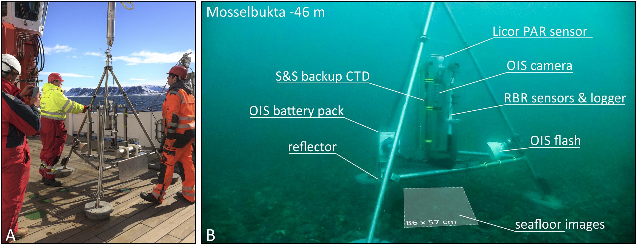
Figure 2. (A) The SaM Lander on board RV Maria S. Merian ready for deployment via winch and acoustic release in June 16th, 2016 in Mosselbukta, Svalbard. (B) The lander and its components photographed with ambient light, sitting on the rhodolith bed at 46 m water depth in Mosselbukta.

The first deployment of the lander took place in Mosselbukta (79° 54.69′ N/15° 48.72′ E), at 46 m water depth (station MSM55/417) in a rhodolith bed with rich and representative associated fauna. The lander was deployed via acoustic release on June 16th, 2016 and delivered 123 h of environmental data and 738 seafloor images, before successful recovery on June 21st. The second deployment was at Bjørnøy-Banken (74° 22.85′ N/19° 27.35′ E), again at 46 m water depth (station MSM55/485) on a rocky hardground with mobile sediment and a representative epibenthic fauna. Here, the lander was deployed on June 23rd and delivered 60 h of data and 361 seafloor images, before recovery on June 26th.

During the lander deployments, relevant meteorological data were measured by the shipboard weather station in 1 min temporal resolution. Absolute wind direction was logged by a Thies Wind Direction Transmitter Classic (accuracy ±2.5°), and absolute wind speed was logged with a Thies Wind Transmitter Classic (accuracy ±0.3 m/s). Surface photosynthetically active radiation (sPAR) was provided by a Biospherical Instruments QSR 2200 PAR sensor as part of a MesSen Nord SMS 1 irradiance measurement platform. During the time of the lander deployment, the vessel was operating in the same working area, less than 15 km from the lander position.

Seafloor Image Analyses

After recovery, all OIS images were batch processed in Adobe Lightroom (v. 5.7.1) with the same setting for exposure and illumination control as well as adjustment of white balance and micro-contrast. In addition, chromatic aberrations were removed and slight sharpening was applied.

Turbidity was not directly measured by sensors on the lander but could be deduced from the OIS images instead. That is, the standard deviation of the grey values of the images served as an inverse proxy for turbidity. Given the fact that all images were captured with the same camera and flash setting, more particles in the water, both between the lens and the object and between the flash and the object, have an effect on the brightness as well as on the range in greyscales of the images. A large range of greyscales, i.e., a more widely scattered histogram leading to a higher standard deviation of the mean grey scale, thus reflects images with darker shadows and brighter lights and, hence, less particles in the water and better water clarity. The respective processing of the images was done using batch measurements of the mean greyscale and standard deviation with the software ImageJ (v. 1.46r).

Macrobenthos Species Inventory

The epibenthic species present on each of the lander images were determined by visual inspection and classified as vagile versus sessile and as calcifier versus non-calcifier. The occurrence of a species on the total image stack of Mosselbukta and Bjørnøy-Banken was assessed according to the following classification: <25%, 25% to 75%, 75% to 100% and 100%.

Feeding Activity

Filter-feeding activity analysis of selected sessile (balanids, serpulids) or semi-sessile (clams, holothuroids) macrobenthos was quantified on a selection of 33 individuals in total from the lander images. Activity and inactivity patterns of each specimen were recorded by visually quantifying the extension and retraction of tentacles (balanids, serpulids and holothuroids) or the opening and closure of the shell/syphon (clams). A binary or trinary code was adopted for each image according to the following rules: x = 1 if the tentacles/syphon or shells were fully expanded/open; x = 0 if the tentacles/syphon or shells were fully retracted/closed; x = 0.5 for intermediate stages (only for Chlamys islandica, Cucumaria frondosa, and Mya truncata). In addition, obvious events that appear to have caused inactivity, e.g., disturbance by mobile epibenthos, were recorded. Mean activity per image and species was calculated as well as a filtering/feeding intermission rate, i.e., the cumulative number of filtering/feeding inactivity events (0 and 0.5 values) per hour.

Spearman rank correlation coefficient ρ, computed with the software SYSTAT (v. 12), was used to describe the relationship between species filtering activity (mean) and abiotic variables derived from the SaM lander measurements (temperature, salinity, pH, photosynthetically active radiation, tide, turbidity). For all comparisons a significance level of α = 0.05 was used.

Mobility Analyses

Mobility analyses of selected mobile macrobenthos species (echinoids, chitons, clams) and passively moved objects (rhodoliths) was performed with ImageJ (v. 1.46) in combination with the ‘manual tracking’ plugin. For that purpose, image stacks of reduced resolution (2000 px) were produced and the individual organisms were manually tracked by marking the centre or a recognisable feature on each frame. Only individuals that were in the field of view for at least 5 frames were considered. The resulting tracks were graphically displayed on a labelled overlay. Compressed versions of these image stacks were exported as AVI movie files (provided as part of the online Supplementary Material). The calibrated results were exported to EXCEL and comprise the distance travelled by each object between two frames and the resulting speed. Since the distance describes a straight line for each 10 min time interval, and since there is no information about vertical movement (rather negligible compared to horizontal movement), the distance and speed values are to be considered conservative estimates. Also, rotation around the tracking point was not recorded. To better characterise the tracked objects, their maximum diameter or length was determined using the measurements tool in ImageJ. The last 23 out of the 738 recorded frames of the Mosselbukta image stack were compromised by accidental dislocation of the lander during video-documentation with the submersible JAGO and were excluded from the analysis. For coherence, the same applies for the feeding activity analysis.

Densities of macrobenthos organisms were normalised from the 86 × 57 frame of observation (∼0.5 m²) to a square metre. Extrapolation to larger areas was considered unfeasible based on the small, albeit representative, window of observation.

Results and Discussion

Seasonality

The 15 months record of temperature and salinity, recorded by the logger on the Mosselbukta settlement platform in summer 2006 to autumn 2007, provides seasonal in situ data for a typical Svalbard rhodolith bed (Figure 3 and Supplementary Table S1 for raw data). Temperature (Figure 3A) followed a slightly left-skewed sinoidal curve. At 46 m water depth in Mosselbukta, bottom water temperatures peaked toward the end of the polar day in August/September with mean values of ∼5°C and a maximum of 6.4°C during a short spike in August 2006. With declining daylight and throughout the polar night (Figure 3E), the temperature decreased to negative monthly means from February to April. Lowest mean (−1°C) and lowest individual record (−1.9°C; basically at the freezing point of seawater) were recorded in April. Accordingly, ice charts indicate the presence of drift ice in Mosselbukta in February and from April to early June 2007 (Figure 3F). The increase in solar irradiation during the polar day is reflected in a rapid increase of the bottom water temperatures from May to early August 2007. Peak summer temperatures were slightly higher in 2006 compared to 2007 but with a consistent timing of the amplitude. Bottom water temperatures at 46 m water depth recorded a decade later by our SaM Lander deployment (see below), are nearly congruent to the 2007 record. Short-term temperature fluctuations were highest in autumn 2006, with shifts of up to 4°C within a few days in late October 2006. This might be a result of increased storm activity inducing mixing of water masses. In general, short-term fluctuations were less than 2°C and were lowest in the warmest months.

FIGURE 3

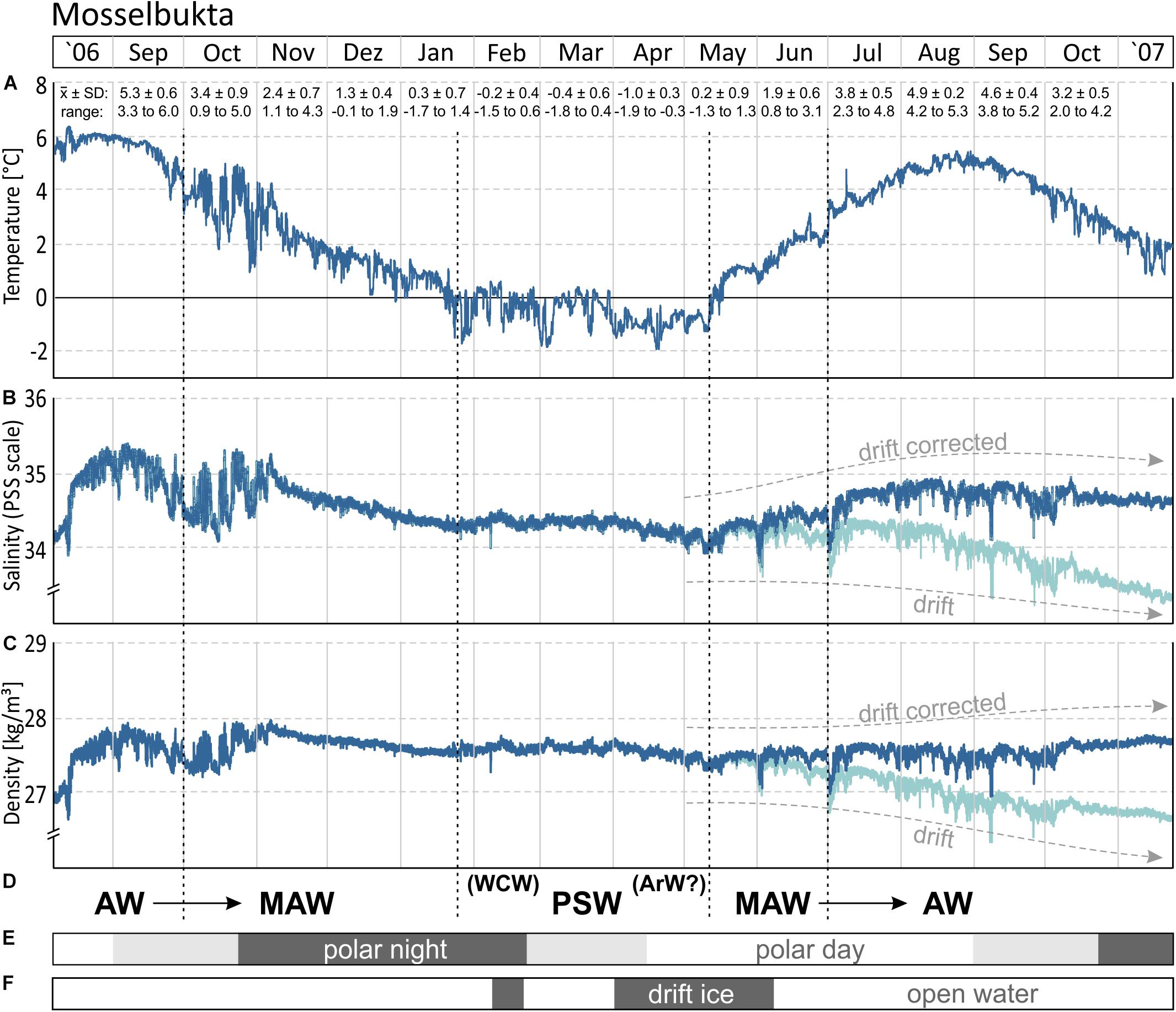
Figure 3. (A,B) The 15-month temperature and salinity record logged by the CT logger on a settlement platform that was deployed in August 2006 at 46 m water depth in Mosselbukta. The decrease during the last 5–6 months in the salinity record likely is a drift artefact (see also Figure 4), for which a drift correction was applied. (C) Seawater density (sigma theta) calculated from temperature and salinity. (D) Determined water mass changes through the investigated period: Atlantic Water (AW), Modified Atlantic Water (MAW), Winter Cooled Water (WCW) and Arctic Water (ArW) contributing to Polar Surface Water (PSW). (E) The duration of the polar night at the study site. (F) The occurrence of open water and closed drift ice in the study area during the deployment in 2006–2007.

The salinity curve is less conclusive (Figure 3B), and a drift artefact toward lower values probably affected the last third of the record. Moreover, the absolute accuracy of the device was relatively low (±0.75 units). Nevertheless, the record gives an impression of the short-term fluctuations that were most pronounced (up to 1 unit) during October 2006, coinciding with the largest temperature fluctuation. Other than that, salinities were rather stable and reflect open ocean conditions with little meltwater influx at the rhodolith beds at 46 m water depth. A drift correction of −0.2 unit per month, beginning in May 2007 (Figures 3B, 4B), draws a more realistic picture and closes the annual cycle (e.g., Harris et al., 1998).

FIGURE 4

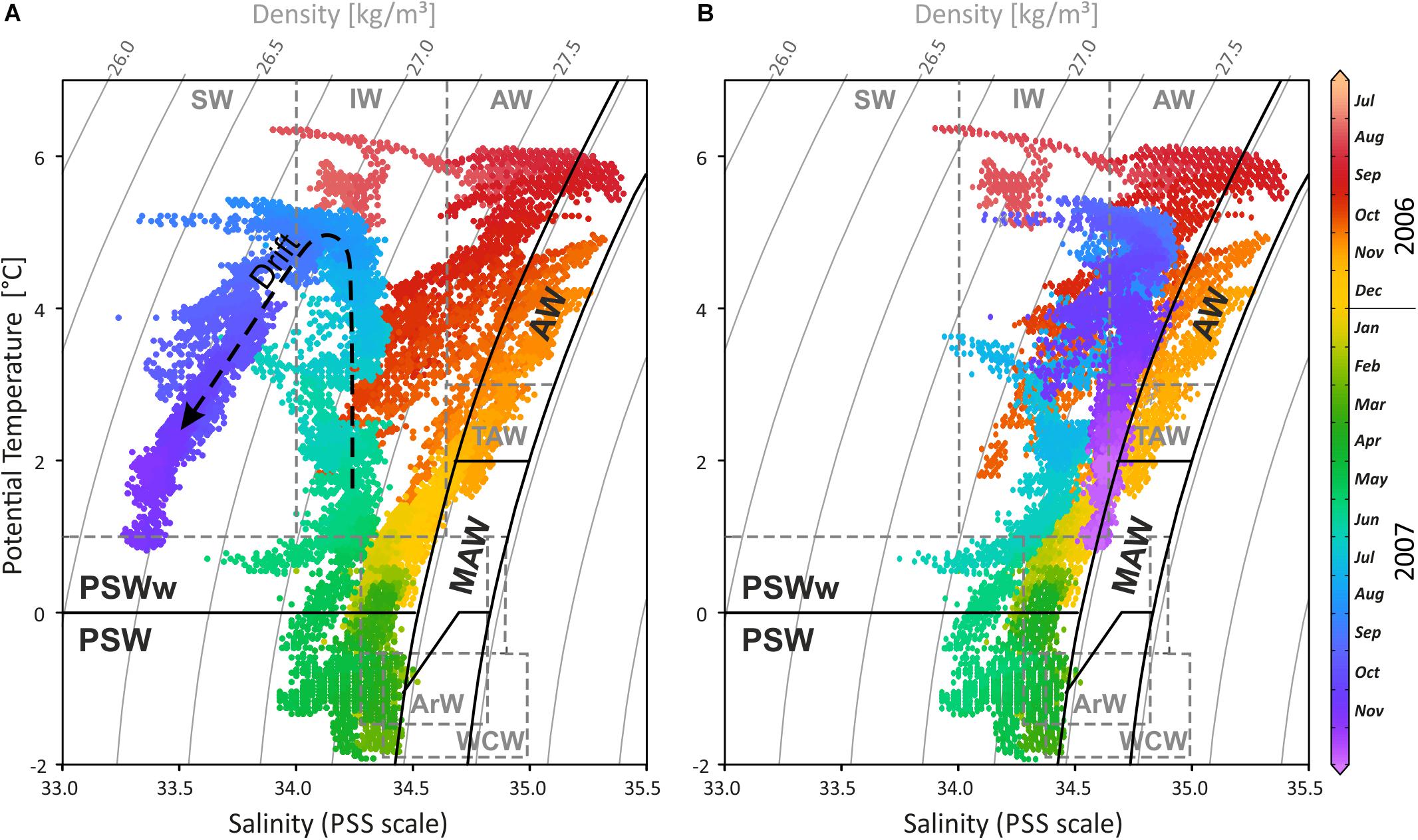
Figure 4. (A) Temperature-salinity-density diagram of the CT logger on the settlement platform, highlighting the temporal variability of water masses during the 15-month record in 2006/2007 (colours correspond to recording time). Waters were cooling and freshening from 6°C in August 2006 down to nearly the freezing point in April 2007 following the mixing line between the external water masses, the Atlantic Water (AW) and the Arctic Water (ArW), forming first Modified or Transformed Atlantic Water (MAW or TAW) and later Polar Surface Water (PSW). During spring and summer 2007 temperatures were increasing while salinity remained low, occupying the TSD field of warm Polar Surface Water (PSWw). As temperatures rised to summer values, salinity decreased further, indicating the drift artefact (dashed arrow). (B) Drift corrected salinity data with –0.2 on the PSS scale per month starting from mid May 2007. Water mass characteristics in black follow Rudels et al. (2000) and in dashed grey Cottier et al. (2005). SW, Surface Water; IW, Intermediate Water; TAW, Transformed Atlantic Water (≅ MAW); WCW, Winter Cooled Water.

Interpreting changing water masses alone from temperature data is not precise (e.g., Rudels et al., 2000) and is therefore based on temperature, salinity, and density (Figures 3D, 4). During late 2006, Atlantic Water (AW) bathed the settlement platform at 46 m in Mosselbukta, cooling during the winter and mixing continuously with Arctic Water (ArW) forming first the Modified or Transformed Atlantic Water (MAW or TAW) and later Polar Surface Water (PSWw or PSW) or even the very cold Winter Cooled Water (WCW) (Rudels et al., 2000; Cottier et al., 2005; see Figures 3D, 4). Slightly fresher waters occurred in Mosselbukta compared to data of Rudels et al. (2000) and Cottier et al. (2005), who describe a mixing line between AW and ArW (here: between AW and PSW, see Figure 4B). Sea ice formation would store fresh water in the ice and salinity would increase in the sea while drifting sea ice would be an additional source of fresh water to Mosselbukta, but this may have not melted during February to April 2007, explaining the lower salinity. Support for this line of reasoning is provided by the stable oxygen isotope signals (see below). However, as the salinity sensor showed a drift (Figures 3, 4A) and accuracy was relatively low, the data should not be over-interpreted, at least for the second half of the long-term exposure.

Short-Term Environmental Variability

The data logged by the SaM Lander, at the same site and depth than the long-term record from the Mosselbukta settlement platform, give insight into short-term fluctuations (tides, temperature, salinity, density, pH, PAR, turbidity) in the carbonate production centre of the rhodolith beds (Figure 5 and Supplementary Table S2 for raw data). A second deployment of the lander at Bjørnøy-Banken allows a comparison of the environmental parameters between the two carbonate factories and provides a basis for interpreting the patterns in macrobenthos dynamics studied by means of sea-floor image time series.

FIGURE 5

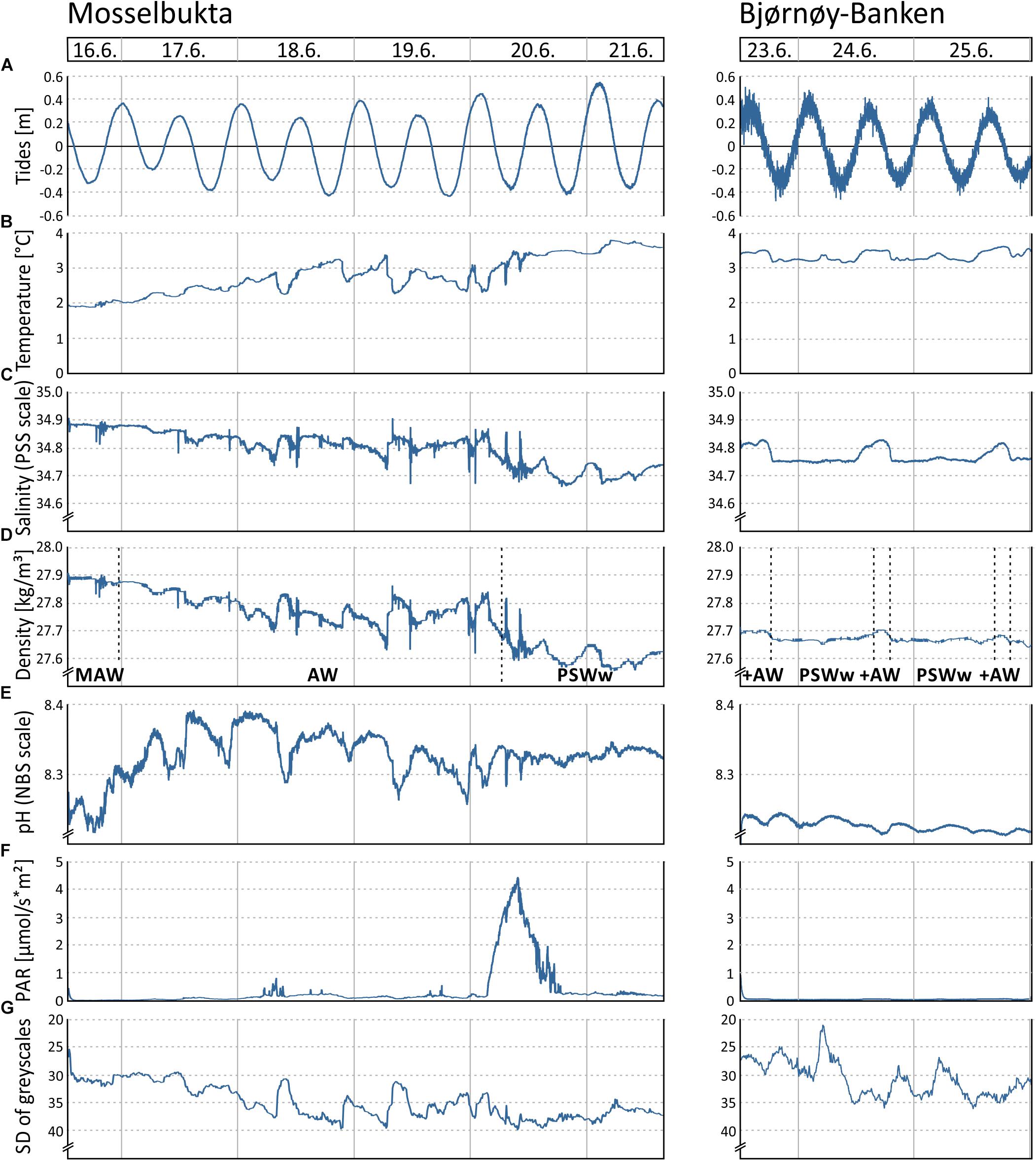
Figure 5. Various environmental parameters recorded by the RBR logger and Ocean Imaging Systems camera on the SaM Lander during two short-term deployments at 46 m water depth in Mosselbukta and at Bjørnøy-Banken, respectively, during the MSM55 cruise in June 2016: (A) Tidal curve (calculated from depth readings). (B) Temperature. (C) Salinity. (D) Seawater density (calculated from temperature and salinity), with indicated water masses of the Atlantic Water from the south (AW), Modified Atlantic Water from the Arctic Ocean (MAW), and warm Polar Surface Water (PSWw). (E) Seawater pH. (F) Photosynthetically active radiation (PAR). (G) Turbidity proxy (standard deviation of mean grey scales in each image of the lander’s camera system).

The tidal range of one metre maximum, recorded by the pressure sensor of the RBR logger (Figure 5A), is similar at both sites. The higher ‘noise level’ in the Bjørnøya data probably is a reflection of the observed stronger bottom currents and higher surface swell. The temperature (Figure 5B) in Mosselbukta increased markedly from around 2°C to about 3.5°C during the 6 days of exposure, reflecting the summer increase that was also seen in the long-term record (Figure 3A). Short-term fluctuations were less than 1°C. At Bjørnøy-Banken, the temperature was more stable and short-term fluctuations did not exceed 0.5°C. The salinity (Figure 5C) shows open ocean values of around 34.8 units on the PSS scale with some short-term fluctuations in the range of 0.2 units in Mosselbukta and less than 0.1 units at Bjørnøy-Banken. In Mosselbukta a slight overall decrease was observed during the 6-day deployment (negatively correlated to temperature), whereas at Bjørnøy-Banken the salinity was more stable with small positive excursions that positively correlated with the temperature fluctuation. Seawater density (sigma theta) data from Mosselbukta decreased from 27.9 kg/m³ at the beginning of the record to values of less than 27.6 kg/m³, thus following largely the variability of salinity (Figure 5D). These data suggest that during June 16th the lander was bathed in Modified Atlantic Water (MAW), later in Atlantic Water (AW), and from June 20th onward in warm Polar Surface Water (PSWw). At Bjørnøy-Banken, in contrast, seawater density data were very stable at around 27.7 kg/m³, indicating the principal influence of PSWw. Slightly higher values of density occurred every second high tide (Figure 5D), accompanied by peaks of temperature and salinity (Figures 5B,C), indicating an influence of AW during high tide that decreased with decreasing tidal amplitude (Figure 5A).

In Mosselbukta, the pH (Figure 5E) did fluctuate between 8.2 and 8.4 units on the NBS scale, whereby the most distinct excursions co-varied with temperature. At Bjørnøy-Banken, pH was lower (ca. 8.2), more stable, and fluctuations were very low. With regard to the photosynthetically active radiation (PAR) (Figure 5F), light levels were surprisingly low, in fact below detection limit for most of the record. Only exception were one short episode of higher light levels and few slight variations in the Mosselbukta record, whereas at Bjørnøy-Banken no PAR was detected. The pronounced peak in Mosselbukta reached a maximum irradiation of about 4.5 μmol/s^∗m² and coincides with the sunniest day while in the working area, reflected also in the highest continuous levels of surface PAR recorded by the vessel’s weather station (Figure 6A and Supplementary Table S3 for raw data). Similar surface conditions at Bjørnøy-Banken did not induce a bottom PAR signal. That is most likely an effect of the higher turbidity (Figure 5G) that is evident from the seafloor images, and also translates into the standard deviation of image greyscales that served as proxy for the turbidity. At Bjørnøy-Banken, the turbidity peaked during ebbing tide and then slowly decreased – a pattern that is interpreted as an effect of resuspension of particles by the strong tidal stream. In Mosselbukta an overall decrease in turbidity over the 6 days exposure was observed, while individual peaks were apparently independent of the tidal rhythm or surface wind direction and speed (Figures 6B,C). The significant southerly wind speeds of up to more than 40 knots measured on June 20th did not have much of an effect on the turbidity, plausibly because this direction is more sheltered by land. The highest turbidity encountered during the first days of the deployment, in contrast, were likely a result of strong northerly winds that passed through during the days before the deployment. This direction faces the open sea, allowing the wind to generate waves and swell capable of affecting the seabed at 46 m water depth.

FIGURE 6

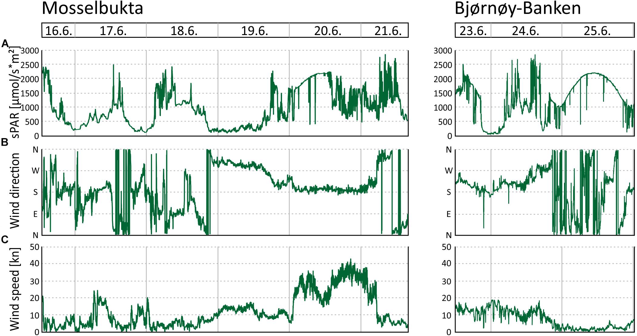
Figure 6. Environmental parameters recorded by the MSM weather station during the period the SaM Lander was deployed at 46 m water depth in Mosselbukta and at Bjørnøy-Banken. (A) Surface level of the photosynthetically active radiation (sPAR). (B) Wind direction. (C) Wind speed.

Water Mass Signatures

The water mass properties based on CTD profiling in Mosselbukta and at Bjørnøy-Banken show small but distinct differences (Figure 7 and Supplementary Table S4 for raw data). Following the definitions of Friedrich et al. (1995) and Rudels et al. (1999), the investigated surface to sub-surface waters belong to AW (Atlantic Water from the south; defined with σ_Θ of 27.70 to 27.97 kg/m³, Θ of >2°C), MAW (Modified Atlantic Water from the Arctic Ocean; σ_Θ of 27.70 to 27.97 kg/m³, but Θ of 0 to 2°C), and PSWw (warm Polar Surface Water formed at or east of the Polar Front; essentially ice melt water above the Atlantic Water; σ_Θ < 27.70 kg/m³ and Θ of >0°C). The more saline waters in Mosselbukta (Figure 7A) indicate the influence of AW at the surface and of MAW from the Arctic Ocean (Rudels et al., 2000) at depth. For both, increasing temperatures and decreasing salinities were recorded over time (dotted arrow in Figures 7A,B) indicating that deeper AW may have an Arctic Ocean source with cooler temperatures, while the shallower waters exhibit a PSWw signature. In contrast, surface waters at Bjørnøy-Banken (Figure 7C) were in average colder and less saline (<34.65) showing a full PSWw signature that has been influenced by less saline polar waters of the Barents Sea. Waters west of the Polar Front are slightly warmer and less saline, implying some AW influence.

FIGURE 7

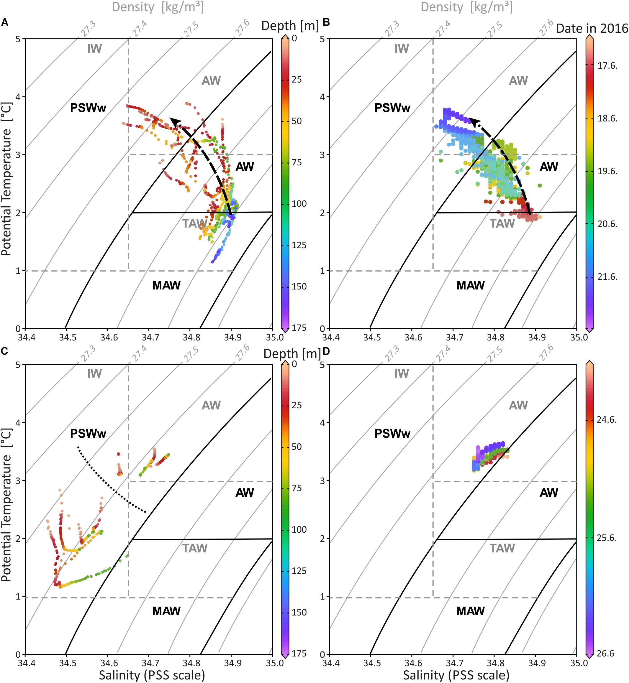
Figure 7. Temperature-salinity diagram including depth and seawater density (sigma-theta) for CTD data of Mosselbukta (A) and Bjørnøy-Banken (C) in comparison with SaM Lander data for same areas, respectively (B,D). Dashed arrow in (A,B) indicates the shift from relatively colder and more saline waters at the beginning of the measurements to warmer and less dense waters 6 days later. Dotted line in (C) separates the data from east (below) and west (above) the Polar Front. Water mass characteristics in black follow Rudels et al. (2000) and in dashed grey Cottier et al. (2005). AW, Atlantic Water from the south; MAW, Modified Atlantic Water from the Arctic Ocean; PSWw, warm Polar Surface Water; IW, Intermediate Water; TAW, Transformed Atlantic Water (≅ MAW).

The SaM-lander data from Mosselbukta are in good agreement with the CTD data (compare Figure 7A and Figure 7B) showing the same trend of increasing temperature and decreasing salinity over time. Here, at 46 m water depth the first TS records from June 17th indicate water with a signature at the transition of MAW and AW (Figure 7B), which progressively exhibits a PSWw signature. At Bjørnøy-Banken, the SaM-lander data at 46 m have a PSWw signature with slight AW influence (Figure 7D). These data are comparable with the CTD data of station 483 situated close to the lander at 55 m water depth.

Time series CTD data of the shallow (46 m) and deep (155 m) stations in Mosselbukta (Figure 8) indicate upwelling waters with a cooler MAW signature at day one (Figures 8A,B), possibly due to strong northerly winds and an influence of the East Spitsbergen Current prior to arrival. During the first 4 days of the lander deployment, winds had switched from SW to SE and died down (Figures 6B,C). The resulting development of stratification to warmer and less saline surface waters with an AW to PSWw signature can also be seen in the salinity and density data (Figures 8C–F). Surface water dissolved oxygen values were highest (>7.3 ml/l) in waters with MAW and AW signature and lowest (min. 6.5 ml/l) for deeper MAW (Figures 8G,H). Fluorescence data closely followed this trend but had maximum values at ∼50 m water depth, strongest in MAW, and decreasing in time (Figures 8I,J). The decreasing trend in surface water oxygen and fluorescence values may indicate a stronger influence of the East Spitsbergen Current bringing PSWw back into this area. Turbidity data show highest values at the seafloor at the deeper station during the first 2 days of exposure (Figure 8K), less pronounced at the shallower station (Figure 8L), indicating the upwelling of MAW during the storm event prior of arrival. The overall decrease in turbidity at depth is mirrored by the indirect turbidity assessment from the SaM-lander (Figure 5G). At the surface, turbidity was low but shows a slight increase with increasing influence of PSWw (Figure 8L), the surface water influenced by melt water around Svalbard, enforced by increased winds (and waves) from a southerly direction during June 20th (Figures 6B,C).

FIGURE 8

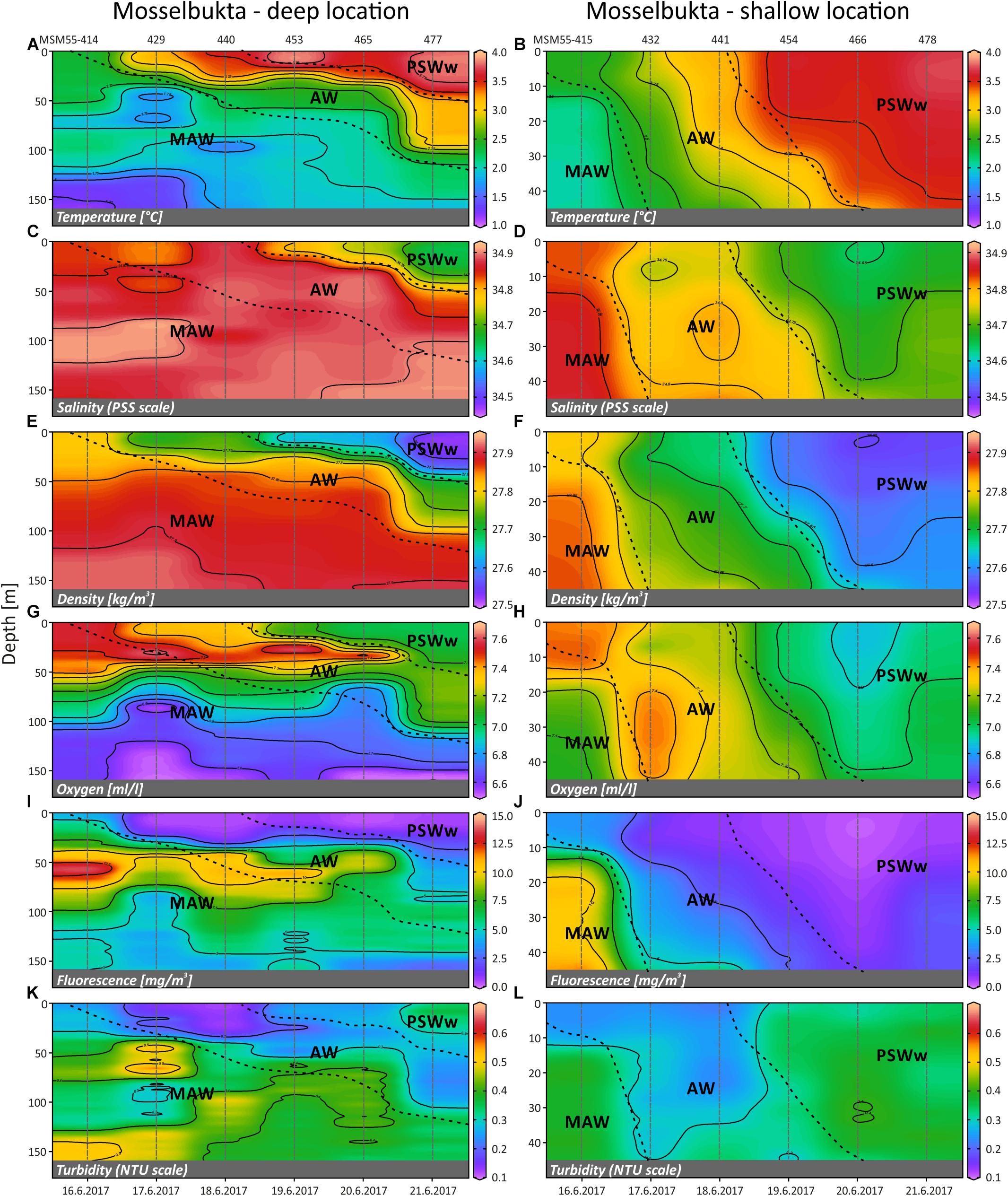
Figure 8. Temperature (A,B), salinity (C,D), density (sigma-theta) (E,F), dissolved oxygen (G,H), fluorescence (I,J) and turbidity (K,L) of the deep (left) and shallow (right) CTD localities in Mosselbukta, plotted against time and water depth (plots generated in Ocean Data View). AW, Atlantic Water from the south; MAW, Modified Atlantic Water from the Arctic Ocean; PSWw, warm Polar Surface Water.

At the Bjørnøy-Banken transect (Figure 9) the Polar Front, separating warmer and more saline waters in the west (PSWw + AW) from cooler and slightly less saline waters in the east (PSWw), is present between CTD stations 514 and 513 with a drop in temperature of ∼1°C (Figure 9A) and in salinity of 0.1 units (Figure 9B), together also evident in the density profile (Figure 9C). Following the characteristics given by Rudels et al. (2000) or Cottier et al. (2005) the waters along this transect can be described as PSWw or local water with an influence of AW west of the Polar Front. This is corroborated by the SaM Lander record (Figure 5D), indicating a small influence of waters with an AW signature during high tides at day time. Dissolved oxygen shows high values (7.2–7.4 ml/l) throughout the transect (Figure 9D), and thus values comparable to AW in Mosselbukta (Figures 8G,H), except for slightly lower values at the Polar Front and the deepest part in the east. Here, under the influence of PSWw, also highest values of >7.4 ml/l were measured at the surface – much higher compared to PSWw in Mosselbukta (<7 ml/l; Figures 8G,H). Fluorescence data show very low values east of the Polar Front, comparable to PSWw in Mosselbukta, while west of the front the influence of AW is visible (Figure 9E). Higher turbidity values of >6 NTU at the coastal area of Bjørnøya decreased eastwards to only 0.2 NTU east of the front (Figure 9F). This pattern can additionally be interpreted as an effect of the tidal cycle, as the highest turbidity observed at the lander site (in 46 m water depth west of the Polar Front) occurred around low tide, when also the CTD casts 483 (shortly before low-tide) as well as 486 and 487 (after low tide) were logged (Figure 9F).

FIGURE 9

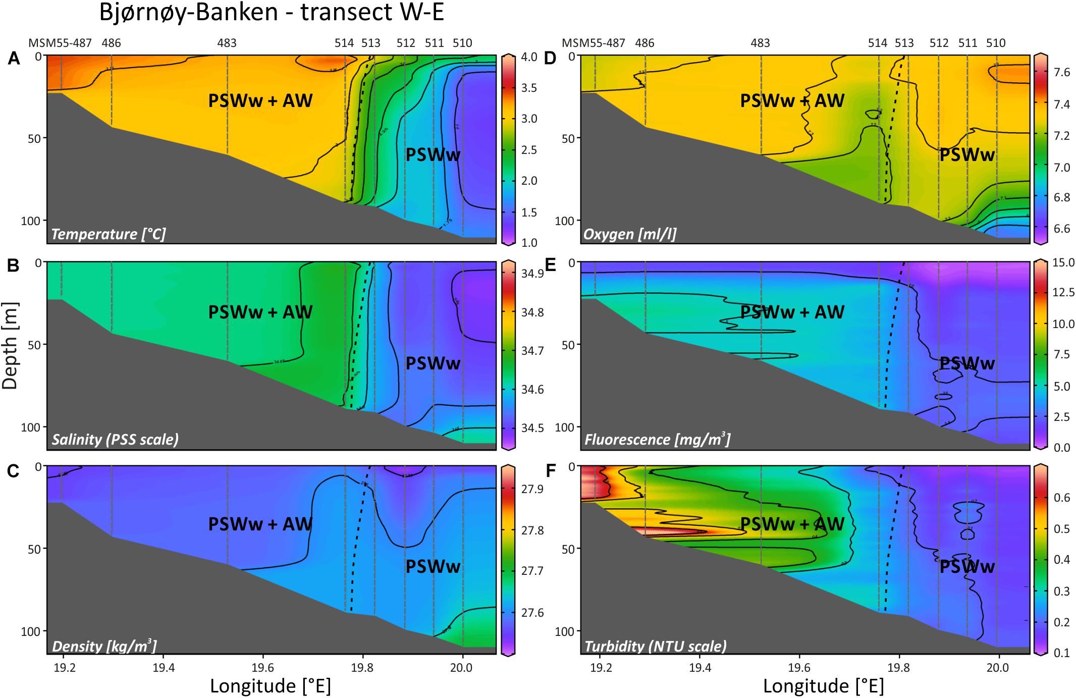
Figure 9. Temperature (A), salinity (B), density (sigma-theta) (C), dissolved oxygen (D), fluorescence (E) and turbidity (F) along a W-E transect SE off Bjørnøya Island, plotted against longitude and water depth (plots generated in Ocean Data View). AW, Atlantic Water from the south; PSWw, warm Polar Surface Water.

Nutrient Regime

The composition of dissolved inorganic nutrients of the ambient seawater, including nitrate (NO₃), nitrite (NO₂), ammonium (NH₄), and phosphate (PO₄), was characterised in surface and bottom waters (Table 2 and Supplementary Table S5 for raw data). While in Mosselbukta, water was sampled regularly at the same two stations (Figure 8), CTD casts at Bjørnøy-Banken were taken along a longitudinal transect across the Polar Front. Results from Bjørnøy-Banken seawater analyses were thus split in a western part (inshore; PSWw + AW) and an eastern part (offshore; PSWw), separated by the Polar Front between stations 513 and 514 (Figure 9).

TABLE 2

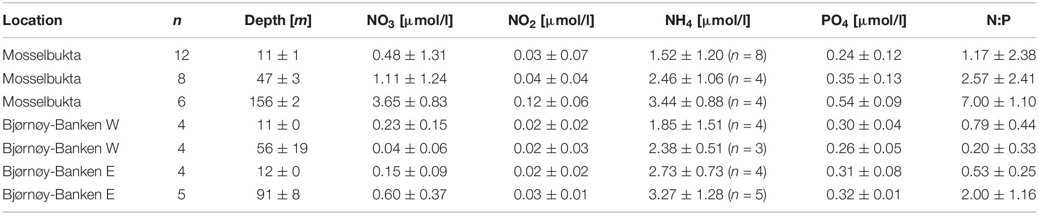
Table 2. Dissolved inorganic nutrients along with Redfield N:P ratios in Mosselbukta and at Bjørnøy-Banken (W and E of the Polar Front) for surface waters and for bottom waters, averaged over the available CTD casts (bottom water stations complemented with water samples taken by JAGO; total number of considered samples per depth indicated in the second column; fewer samples for ammonium indicated in the respective column).

In Mosselbukta, concentrations of all nitrogenous nutrients were relatively low (<4 μmol/l), but consistently increased toward depth with levels at least doubling compared to surface waters. N:P ratios likewise increased with depth from just above 1 in surface waters (mainly AW and PSWw) to 7 at about 150 m water depth (MAW).

At Bjørnøy-Banken the dissolved inorganic nutrients showed a different pattern with depleted nitrate and nitrite levels compared to Mosselbukta, resulting in lower Redfield N:P ratios. The comparison of surface and bottom waters did show a systematic increase of the dissolved inorganic nutrient levels and N:P ratios with depth in the PSWw east of the Polar Front, and an inconclusive pattern in the shallower inshore PSWw + AW.

Nitrate concentrations were comparable to values from Kongsfjorden at similar depths end of May 2002 (Hodal et al., 2012). Nitrate and phosphate concentrations of the first 50 m in Kongsfjorden in May 2006 also matched our results from Mosselbukta (Iversen and Seuthe, 2011). In comparison to the other months, especially April, nutrient concentrations in May to July were substantially lower in Kongsfjorden in 2006 (Iversen and Seuthe, 2011; Hodal et al., 2012), indicating nutrient depletion after the spring bloom, and thus the state of a post-bloom phase in May/June.

High ammonia concentrations in comparison to low amounts of nitrate and nitrite, especially in the upper 50 m of Mosselbukta, might indicate a recycling system fuelling primary production (providing nutrition for zooplankton and benthic filter-feeders feeding upon it) after the spring bloom, which has also typically been described in the Kongsfjorden for this time of the year (June; Iversen and Seuthe, 2011; Schulz et al., 2013). The same interpretation applies for the even more pronounced depletion of nitrogenous nutrients in surface and bottom waters from both sides of the Polar Front at Bjørnøy-Banken. The less pronounced bathymetrical increase, compared to Mosselbukta, is seen as a result of mixing induced by the strong tidal currents observed during the cruise, particularly west of the Polar Front.

Carbonate System

The measured carbonate system parameters TA and DIC are differentiated in development across the different water masses in both locations. While TA was constant in Mosselbukta throughout the water column from 11 to 156 m, with an overall mean of 2312.4 ± 8.8 μmol/kg_SW (n = 26), DIC increased with depth with a shift of ∼90 μmol/kg_SW from the surface to the bottom at the deeper station (Table 3 and Supplementary Table S5 for raw data). The shift in DIC toward higher values in the deeper water layers is likely a result of decreasing water temperatures and/or consumption of CO₂ in the upper water layers by the plankton community. The calculated carbonate system parameters pH, pCO₂, and the saturation states for calcite (Ω_Ca) and aragonite (Ω_Ar) are in accordance with the trends in DIC. The omega values as well as pH decrease with depth in Mosselbukta (by about 0.14 units), as do the saturation states, while the CO₂ concentration increases (by about 80 μatm) from 11 to 156 m (Table 3).

TABLE 3

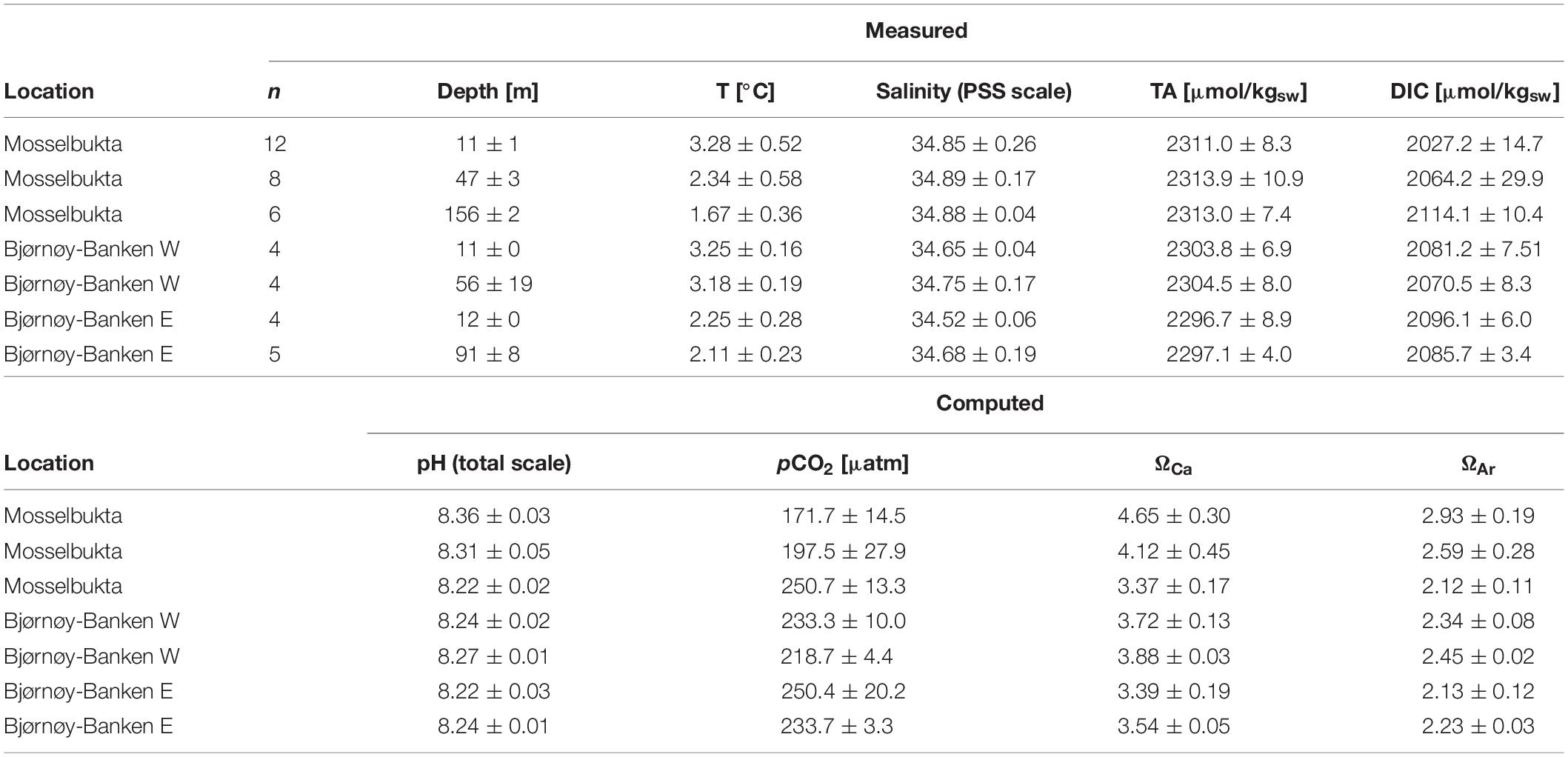
Table 3. Measured and computed carbonate system parameters in Mosselbukta and at Bjørnøy-Banken (W and E of the Polar Front) for surface and bottom waters, averaged over the available CTD casts (bottom water stations complemented with water samples taken by JAGO; total number of considered samples per depth indicated in the second column).

At Bjørnøy-Banken, TA values were only slightly lower, with an overall mean of 2300.3 ± 7.4 μmol/kg_SW (n = 17), but likewise similar across all depths, while a drop in DIC with depth (by ∼20 μmol/kg_SW) was only evident in the PSWw + AW west of the Polar Front. This drop was observed in spite of homogenous temperatures (Table 3). In contrast to Mosselbukta, lower pH values were found in the surface waters, and a slight increase with depth was recorded both sides of the Polar Front. Accordingly, pCO₂ levels and Ω values varied only very slightly.

As a general observation, pCO₂ levels were remarkably low at both study sites, far below global present-day equilibrium values, with overall means of only 197.4 ± 37.0 μatm (n = 26) and 234.0 ± 15.1 μatm (n = 17) in Mosselbukta and at Bjørnøy-Banken, respectively. The lowest values (171.7 ± 14.5 μatm) were recorded in the surface waters in Mosselbukta. These low carbon dioxide concentrations, in concert with elevated oxygen levels (Figure 8G) and the depletion in N and P nutrients (see above), are interpreted as an effect of a boost in community photosynthesis during phytoplankton spring bloom in combination with the onset of rhodophyte photosynthesis during the polar day upon retreat of sea-ice. Very similar values of pCO₂ (170 μatm) and a corresponding pH of 8.35 were observed during a post-bloom phase in Kongsfjorden in western Spitsbergen in June 2010 (Schulz et al., 2013). Experiments carried out in the West Svalbard Shelf (Sanz-Martín et al., 2018) suggest that such episodic Arctic CO₂ limitations, together with nutrient depletion, may contribute to the termination of the Arctic spring plankton blooms. We interpret this pattern to be further enhanced by the reduction in air-sea gas exchange during seasonal ice cover, which is a particularly pronounced phenomenon in Mosselbukta. The relevance of this effect for the Arctic Ocean has recently been demonstrated by Islam et al. (2016), and we would thus expect this seasonal feedback mechanism to apply also to other polar carbonate factories, such as in the Canadian Arctic or in the Southern Ocean.

In contrast, 13 samples taken in August 2006 during the MSM2-3 expedition in northern Svalbard at or near sites with rhodolith beds, including Mosselbukta (Teichert et al., 2012, 2014), show pCO₂ values close to expected equilibrium values but exhibiting strong variability (overall mean: 406.3 ± 139.7 μatm), indicating partial to complete re-equilibration by that time of the year. As a consequence, pH values (8.03 ± 0.13 on total scale) and saturation states for calcite (2.35 ± 0.61) and aragonite (1.48 ± 0.38) were considerably lower, albeit always saturated at sites of rhodolith growth (Teichert et al., 2014). In June 2016, waters were well-saturated (overall means of 4.19 ± 0.61 and 2.64 ± 0.38 in Mosselbukta, and 3.63 ± 0.21 and 2.28 ± 0.13 at Bjørnøy-Banken), suggesting little effects, if any, of physicochemical carbonate dissolution on marine calcifiers. Hence, the adverse effects of ocean acidification that are predicted to be particularly relevant for circumpolar calcifiers (see AMAP, 2018 for the latest review) can be expected to be buffered to some extend by the marked annual drop in pCO₂ during the phase of seasonal sea-ice cover and spring plankton bloom, and the phase of re-equilibration thereafter. However, this effect will diminish if the degree of seasonal sea-ice formation continues to decline at the present rate (Hetzinger et al., 2019).

Stable Carbon Isotopes of Dissolved Inorganic Carbon

The stable carbon isotopic composition of DIC (δ¹³C_DIC) in the marine realm is influenced both by biological processes and by air-sea exchange of CO₂ and is therefore not easily constrained (Kroopnick, 1985). During photosynthesis, organisms preferentially incorporate the lighter ¹²C and thereby increase the δ¹³C_DIC of the ocean’s surface waters. At depth, remineralisation of the isotopically light organic material leads to a decrease in the δ¹³C_DIC (Broecker and Maier-Reimer, 1992). This parallels the gradient of dissolved inorganic nutrients, which usually are more depleted in surface waters and increase in concentration at depth. If the δ¹³C_DIC of the oceans were only controlled by this process, δ¹³C_DIC would decrease by 1.1 ‰ per 1 μmol/kg PO₄ (Broecker and Maier-Reimer, 1992).

We analysed δ¹³C_DIC of a total of 43 seawater samples from Mosselbukta and Bjørnøy-Banken (Table 4, Figure 10, and Supplementary Table S5 for raw data), taken in surface waters and above the seafloor, to understand to what degree sea-ice and CO₂ uptake (air-sea exchange) related processes around Spitsbergen influence the levels of δ¹³C_DIC. Together with the determined δ¹⁸O_sw these data furthermore provide a baseline for future carbonate stable isotope analysis of marine calcifiers in the Svalbard carbonate factories.

TABLE 4

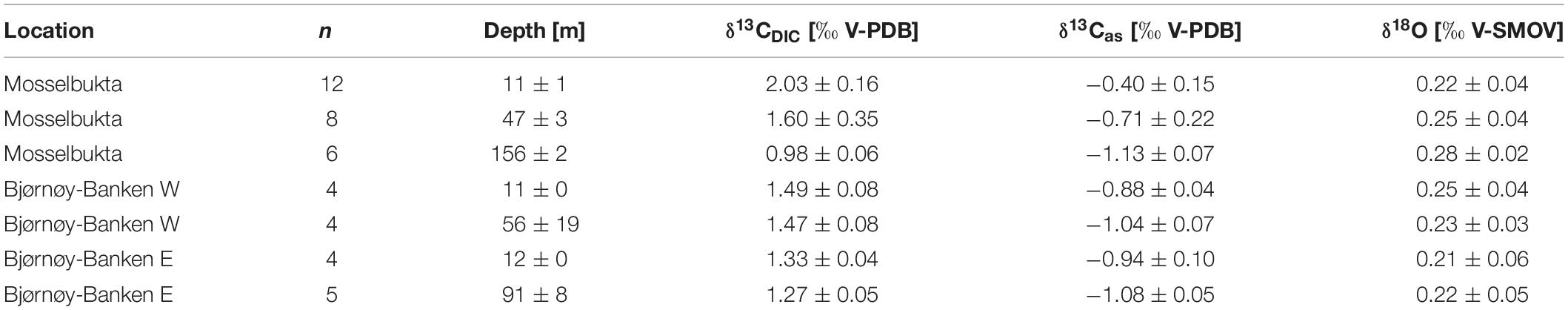
Table 4. Stable isotope and DIC values in Mosselbukta and at Bjørnøy-Banken (W and E of the Polar Front) for surface waters and for bottom waters, averaged over the available CTD casts (bottom water stations complemented with water samples taken by JAGO; total number of considered samples per depth indicated in the second column).

FIGURE 10

Figure 10. Stable carbon and oxygen isotopes of dissolved inorganic carbon in seawater samples taken from Mosselbukta and Bjørnøy-Banken. (A) δ¹³C_DIC plotted against water depth. (B) δ¹³C_DIC plotted against PO₄ concentrations, including the δ¹³C_DIC – PO₄ relationship from various Arctic regions compiled by Bauch et al. (2015). (C) Adjusted δ¹³C_as calculated after Lynch-Stieglitz et al. (1995) and plotted against pCO₂ (for details see text). (D) δ¹⁸O_sw plotted against water depth. (E) δ¹⁸O_sw plotted against seawater salinity. (F) Same as E but including the δ¹⁸O_sw - salinity relationships from Kongsfjorden (W Spitsbergen, MacLachlan et al., 2007) and Sognefjorden (W Norway, Mikalsen and Sejrup, 2000).

In Mosselbukta the δ¹³C_DIC values decrease with water depth and vary on average from 2.03‰ in surface waters (∼11 m), over 1.60‰ for bottom waters of intermediate depth (∼47 m), to 0.98‰ for bottom waters at the deeper station (∼156 m), being possibly a reflection of the different ambient water masses PSWw, AW and MAW, respectively (Figure 7). At Bjørnøy-Banken, such a large spread was neither found when comparing surface and bottom waters, nor between waters west (PSWw) and east (PSWw + AW) of the Polar Front (Figure 8), which appear to have a rather similar carbon isotope signal (1.49 to 1.47‰ vs. 1.33 to 1.27‰, respectively). Combining data from both sites, an overall decrease in δ¹³C_DIC from surface to depth (Figure 10A) is evident. Such a systematic δ¹³C_DIC–depth gradient is consistent with the aforementioned remineralization process, as it is also suggested by the close relationship of δ¹³C_DIC with nutrient concentrations, here PO₄ (Figure 10B). Even though the range of PO₄ is relatively small, varying from 0.1 to 0.6 μmol/kg, it is consistent to the Arctic δ¹³C_DIC - nutrient relationship of Bauch et al. (2011). However, our data exhibit a change of 1‰ per 0.5 PO₄ μmol/kg (Figure 10B), being two times stronger as if only biological processes would affect the δ¹³C_DIC. According to that, it is also possible to determine to what degree also air-sea processes influence the δ¹³C_DIC by adjusting to their nutrient level. Due to the phosphate limitation around Spitsbergen we here use the PO₄ approach of Lynch-Stieglitz et al. (1995), by calculating the adjusted δ¹³C_as using the following equation δ¹³C_as = δ¹³C_DIC - (2.7 - 1.1 ^∗ PO₄). This method subtracts the δ¹³C values predicted from biological activity alone from the actual δ¹³C_DIC assuming that all non-biotic factors are related to air-sea exchange processes. This approach is based on ideal biological processes with a constant fractionation and constant Redfield nutrient ratio (Lynch-Stieglitz et al., 1995; Bauch et al., 2015). We are aware that this approach is not adjusted to local Arctic conditions (see Table 2 for the observed variation in N:P), but it nevertheless gives an indication to what degree air-sea exchange processes control the δ¹³C_DIC distribution around Spitsbergen.

The resulting δ¹³C_as values (Table 4) reveal a relatively large range between −0.1 and −1.2 ‰. The detailed study by Bauch et al. (2015) showed that air-sea exchange processes in the entire Arctic Ocean and shelf regions are far from being at equilibrium, implying that at high latitudes diffusion of CO₂ from the atmosphere into the oceanic system leads to a decrease in δ¹³C_DIC and δ¹³C_as (Lynch-Stieglitz et al., 1995). This is also consistently identifiable in the present relationship between pCO₂ and δ¹³C_as values (Figure 10C). Mosselbukta in particular shows a considerable range in pCO₂ and δ¹³C_as values with a clear trend toward lighter δ¹³C_as values with depth. In comparison Bjørnøy-Banken is characterised by relatively light δ¹³C_as values, which tend to only slightly decrease with depth and higher pCO₂ concentrations.

Relatively high (close to 0 ‰) δ¹³C_as values in Mosselbukta can be explained by an inhibition of air-sea exchange at shallow depth arising from longer and more complete ice coverage compared to Bjørnøy-Banken (Stein et al., 2017)⁴. Lighter δ¹³C_as values (∼−1‰ similar to the North Atlantic, Lynch-Stieglitz et al., 1995) at greater depth in Mosselbukta and at Bjørnøy-Banken instead may result from brine rejection during sea-ice formation and a relatively strong invasion of atmospheric CO₂ associated with sinking cold water, respectively. This is consistent with low δ¹³C_as on Arctic shelf areas, mainly reflecting the invasion of isotopically light atmospheric CO₂ under non-equilibrium conditions (Bauch et al., 2015).

Stable Oxygen Isotopes of Seawater

Stable oxygen isotopes of seawater (δ¹⁸O_sw) have been shown to be a useful tracer to track freshwater influence and sources, especially in high-latitude settings (Bauch et al., 1995, 2011; Cooper et al., 2008). This is owing to the fact that sea-ice is slightly enriched, whereas Arctic meteoric waters are strongly depleted in its oxygen isotopic composition relative to seawater (Bauch et al., 1995). Furthermore, oxygen isotope mixing lines are particularly useful as they can be used to characterise water mass formation (Bauch et al., 2005). Such mixing lines aim to constrain the controlling factors of the oxygen isotopic composition of seawater and subsequently can be used for palaeoceanographic reconstructions.

Here, we have analysed 43 seawater samples for stable oxygen isotopes in Mosselbukta and at Bjørnøy-Banken, covering a salinity range from 34.4 to 35.7 (Table 4, Figure 10, and Supplementary Table S5 for raw data). The δ¹⁸O_sw values in Mosselbukta and at Bjørnøy-Banken exhibit a relatively small range, between 0.16 and 0.31‰ and from 0.18 to 0.28‰, respectively (Figure 10D). Both areas plot close to the global average of ∼0 ‰ for seawater (Schmidt et al., 1999: Global seawater oxygen-18 database)⁵. In contrast to water depth (Figure 10D), salinity reveals an influence on δ¹⁸O_sw values (Figure 10E) and fit to the global δ¹⁸O_sw – salinity relationship of Schmidt et al. (1999: Global seawater oxygen-18 database) (see foot note). Even though the observed range in δ¹⁸O_sw values are within analytical uncertainty, a strong relationship between δ¹⁸O_sw and salinity is apparent in Mosselbukta (r² = 0.8; Figure 10E). This relationship may represent a first order mixing between more saline MAW and AW with fresher PSWw at shallower depth (see also Figure 8), possibly being enhanced by glacial or sea-ice melt. Any deviation of this mixing line toward lower or higher salinity values at constant δ¹⁸O_sw indicate sea-ice melt (lower values) or sea-ice formation (higher values: with associated brine release; Bedard et al., 1981). In Mosselbukta, three samples exhibit values above 35 on the PSS scale (Figure 10E), with δ¹⁸O_sw values deviating from above δ¹⁸O_sw – salinity relationship. These values might be associated with previous periods of sea-ice formation and consistent with the interpretation of the δ¹³C_as values. Consequently, these values were omitted from the computation of a δ¹⁸O_sw – salinity relationship described by the following equation: δ¹⁸O_sw = 0.53 ^∗ S - 18.09. Such a relationship is not apparent at Bjørnøy-Banken. Here, the δ¹⁸O_sw values reveal a similar variability of 0.15‰ as in Mosselbukta, but no clear relationship to salinity. This might be explained by different end-members (latitude effect) of the two different water masses influencing the oxygen isotopic composition west and east of the Polar Front (Figure 8). That is, the PSWw + AW west of the Polar Front is rather warm, slightly more saline, and of southern origin, whereas the PSWw in the east is rather cold, less saline, and of northern origin, and these differences are reflected in the different δ¹⁸O_sw signals_.

The Mosselbukta δ¹⁸O_sw – salinity relationship fits in well with those previously described by MacLachlan et al. (2007) from Kongsfjorden in western Spitsbergen and by Mikalsen and Sejrup (2000) from Sognefjorden in western Norway (Figure 10F). As the Sognefjorden is located at lower latitude and is influenced by different end-members, it may only partly be comparable to the Svalbard setting, but it adds on missing salinity values of around 33 (PSS). The Mosselbukta δ¹⁸O_sw – salinity relationship appears to be slightly steeper (0.5263) compared to Mikalsen and Sejrup (2000) and MacLachlan et al. (2007). Unfortunately, we do not have a Mosselbukta freshwater end-member at hand to verify this. However, taking all three mixing lines together (Figure 10F) the relationship can be described by equation δ¹⁸O_sw = 0.36 ^∗ S - 12.30. This would indicate a freshwater end-member of −12.30, which is slightly higher than the −14.35 obtained by MacLachlan et al. (2007), but very similar to that of Mikalsen and Sejrup (2000) with −12.51 (Figure 10F). In conclusion, our approach demonstrates a relatively robust δ¹⁸O_sw – salinity relationship despite the complex oceanographic systems, and our additional data adds coherently to already existing data and may be used as a Svalbard system specific δ¹⁸O_sw – salinity calibration down to salinity values of 30. The analysis of water samples from other fjords and freshwater end-members in Svalbard is needed to solidify this relationship.

Macrobenthos Diversity

A total of 25 taxa were identified from the image stacks of the lander’s camera system with crustaceans (6 taxa), echinoderms (6) and molluscs (6) as dominating groups, representing 72% of the identified species (Table 5 and Figures 11, 12). Nineteen taxa could be determined to species level and six to genus level, although that high identification rate was only possible by the help of parallel beam trawl catches (see Wisshak et al., 2017 for detail). Most taxa in Mosselbukta as well as Bjørnøy-Banken were vagile calcifiers and could be identified on every image (presence 100%). Diversity was much higher in Mosselbukta (21 taxa) compared to Bjørnøy-Banken (8 taxa), which is most likely due to the occurrence of Lithothamnion glaciale rhodoliths in Mosselbukta covering about 50% of the seafloor visible in the lander images (Figure 11). This is in line with the fact that L. glaciale is considered a bioengineer, which forms characteristic three-dimensional habitat structures that promote benthic biodiversity by providing substratum, protection and food for other benthic organisms (Teichert et al., 2012, 2014). On the other hand, differences in species diversity might not only be depth and substrate dependant (as applying also for Kongsfjorden; see Sahade et al., 2004), but also related to environmental factors such as salinity, temperature or turbidity. As demonstrated above, environmental conditions and water masses between Mosselbukta and Bjørnøy-Banken differ markedly, therefore promoting different fauna and species richness.

TABLE 5

Table 5. Macrobenthos species inventory of organisms identified in the image stacks of the lander’s camera system, with reference to the location (M, Mosselbukta; B, Bjørnøy-Banken), their motility, and their temporal presence in four percent classes.

FIGURE 11

Figure 11. Selected seafloor images (field of view = 86 × 57 cm) taken by the lander’s camera system during the 6 days of deployment at 46 m water depth in the rhodolith belt in Mosselbukta: (A) Last image in the series, with labels for those species that have either been tracked and/or analysed for feeding activity. (B) First image in the series; note the marked difference in turbidity and thus image contrast. (C) Last image in the series with the labelled tracks of the Lithothamnion glaciale rhodoliths. (D) Last image in the series with the labelled tracks of the echinoid Strongylocentrotus sp., the main agent of moving around rhodoliths. (E) Another trigger for movement of rhodoliths and other organisms is the great spider crab Hyas araneus.

FIGURE 12

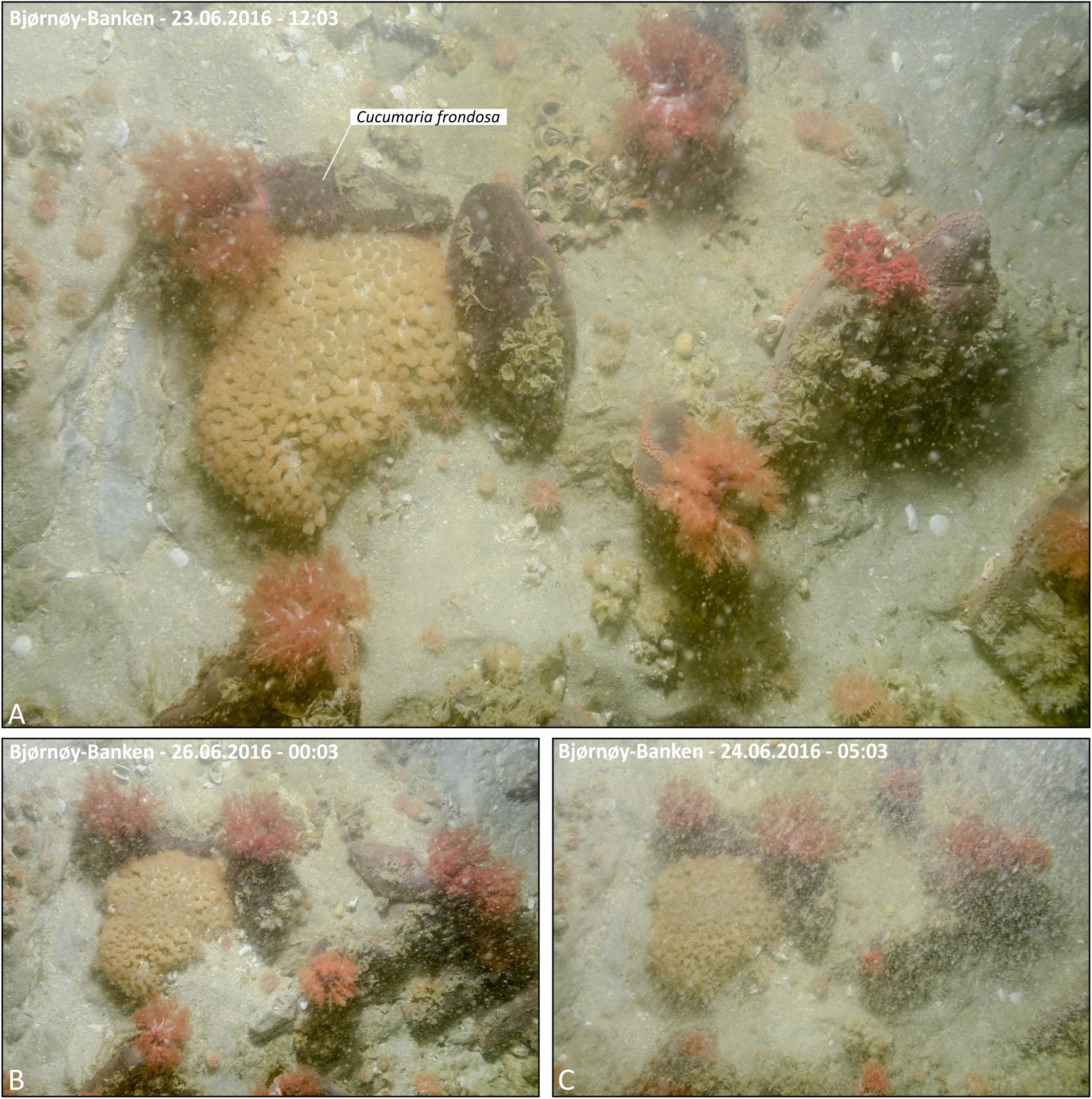
Figure 12. Selected seafloor images (field of view = 86 × 57 cm) taken by the lander’s camera system during the 3 days of deployment at 46 m water depth on the carbonate platform at Bjørnøy-Banken: (A) First image in the series with several specimens of the large holothuroid Cucumaria frondosa, which was analysed for feeding activity. (B) Last image in the series for comparison. (C) An image taken during one of the tidal-induced phases with high currents and turbidity, leading to low contrast images, and prohibiting analysis of feeding activity except for the large holothuroids.

Macrobenthos Dynamics – Feeding Activity

Filtering activity of a total of 26 individuals was investigated in Mosselbukta. The individuals belong to balanids (Balanus sp.; 8 ind.), serpulids (Serpula sp.; 8 ind.), as well as epibenthic bivalves (Chlamys islandica; 6 ind.) and endobenthic bivalves (Mya truncata and Hiatella arctica; 4 ind.). Generally, individuals were more active than inactive throughout the study period, but results reveal no common activity pattern between species (Figure 13). For instance, serpulids and C. islandica were more inactive in the last 2 days (Figures 13C,D,G,H), while for balanids a pronounced phase of inactivity was found from the third to fifth day (Figures 13A,B). Filter-feeding by M. truncata and H. arctica was very homogenous during the study period with no obvious activity pattern (Figures 13E,F). The investigated individuals were often disturbed during filtering in Mosselbukta due to the high population density of mobile epifauna in that habitat (Figures 13A,C,E,G). Among the nine species that caused disturbances, hermit crabs were the most common troublemakers.

FIGURE 13

Figure 13. Mean filter-feeding activity and cumulative intermissions in activity per hour of selected benthos organisms, as observed on images of the lander’s camera system during the 6 days of deployment in Mosselbukta: balanids (A,B), serpulids (C,D), endobenthic bivalves (E,F), and epibenthic bivalves (G,H). Abbreviations used for indicating disturbances: E, echinoid; O, ophiuroid; A, asteroid; C, crab; S, shrimp; H, hermit crab; B, bivalve; G, gastropod; F, fish.

To evaluate possible correlation of macrobenthos filtering activity to the environmental parameters logged by the SaM Lander, Spearman rank correlation coefficients were computed. No significant correlations were found, except for a moderate negative correlation between mean activity of serpulids and temperature in Mosselbukta (ρ = −0.370, P < 0.001). This observation is consistent with our observations that serpulids are more sensitive to external influences than the other species studied. With regard to the involved water masses, this indicates that serpulids are more inactive in the presence of warm Polar Surface Water (PSWw) and more active, when MAW or Atlantic Water (AW) dominates (Figures 3A, 8A,B, 13C,D). Possibly, this is an effect of different load in particulate organic matter (POM) serving as source of food for the filter-feeding organisms, but we do not have data to verify this. In any case, in the densely populated Mosselbukta rhodolith beds, the influence of disturbance by other individuals on the filtering activity seems to be greater than abiotic factors during the 6 days of observation.

As for Bjørnøy-Banken, seven individuals of the holothuroid Cucumaria frondosa were analysed regarding their filtering activity. It is assumed that our observations were made within the main feeding period of C. frondosa, which is in spring and summer (Hamel and Mercier, 1998; Singh et al., 1999). The population density of C. frondosa was very high during the sampling period at Bjørnøy-Banken with up to 363 individuals/200 m² caught in parallel beam trawl hauls and 7 individuals captured within the 86 × 57 cm sized field of view at the randomly selected lander site. Moderate correlations were found between mean filtering activity of C. frondosa and the turbidity proxy (ρ = −0.352, P < 0.001), tidal cycle (ρ = 0.330, P < 0.001), as well as pH (ρ = −0.350, P < 0.001), while the latter is likely indirect only and reflects the tidal rhythm of the involved water masses. Thus, C. frondosa revealed highest filtering rates during high tide at Bjørnøy-Banken when turbidity is comparatively low (Figure 14). Turbidity is not interpreted as a proxy for available food for C. frondosa in this study. Instead, the lander’s sea floor images reveal that high turbidity during ebbing and low tide is associated with the turbulence of sand and other particles at high flow velocities, which most likely reflect unfavourable feeding condition and results in low filtering activity of C. frondosa (Figures 12C, 14). This result fits well to the findings of Singh et al. (1999) who also found a decreasing feeding rate of C. frondosa at too high current speed and low food concentration in the Bay of Fundy, Canada. C. frondosa is a passive suspension feeder whose feeding depends on currents moving water through their filtering tentacles (Singh et al., 1998). However, the feeding rate of C. frondosa is determined by an optimal combination of capture efficiency, rate of particle encounter, and the deformation of the feeding elements, which in turn is determined by current speed (Singh et al., 1999). High current speed can result in the deformation of the feeding tentacles (as observed in our sea-floor images), which might result in a reduction of surface area available for particle capture. Furthermore, the physical resistance on tentacle movement into the mouth can increase with increasing flow velocities (Singh et al., 1999). Together with a low food concentration at high flow rates, these may be reasons for the observed low filter activity just before low tide. In general, the interaction between current flow and food quantity/quality seems to be the most important factor for many suspension-feeding species (Jørgensen, 1966) and can possibly be regarded as a general phenomenon. In the English Channel, for example, a perfect match between turbulence and resuspension was essential for the suspension feeding brittle star Ophiothrix fragilis (Davoult and Gounin, 1995) and also suspension feeding of the crinoid Antedon mediterranea depends on the ambient particle concentration and current speed (Leonard, 1989). We therefore conclude that the best feeding conditions for C. frondosa with regard to food concentration, food quality and current speed were found during high tide at Bjørnøy-Banken when flow velocity and turbidity was relatively low.

FIGURE 14

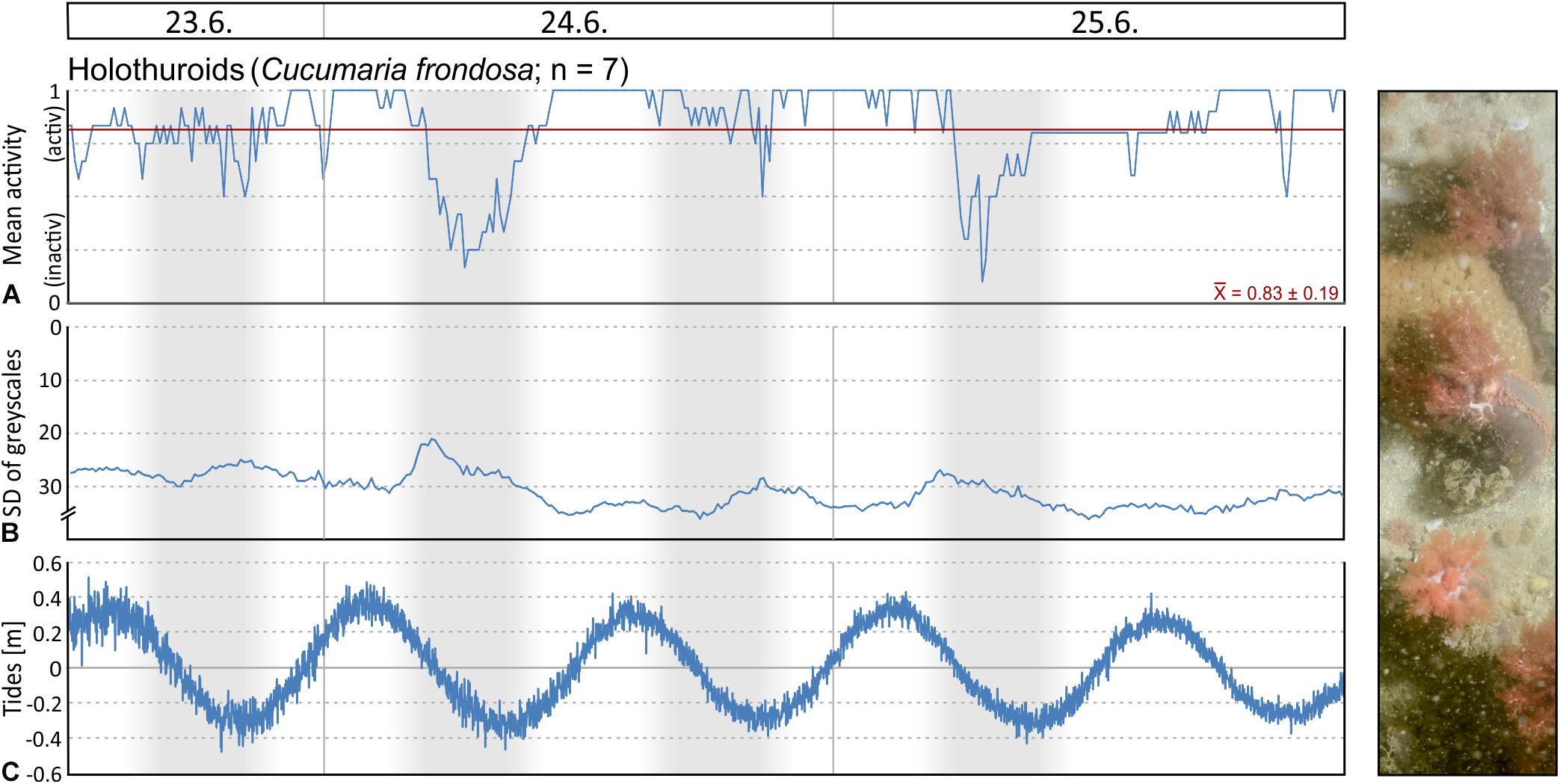
Figure 14. (A) Mean filter-feeding activity and cumulative intermissions in activity per hour of holothuroids observed on images of the lander’s camera system during the 3 days of deployment at Bjørnøy-Banken. (B) Turbidity proxy (standard deviation of mean grey scales in each image). (C) Tidal curve; note the correlation to the feeding activity.

Macrobenthos Dynamics – Mobility Analysis

As an expression of the sedimentary dynamics in the local carbonate factory, 28 Lithothamnion glaciale rhodoliths (= 57 individuals per m²), 4.2 to 12.8 cm in size and with a mean of 7.7 ± 2.0 cm, were tracked with respect to their passive dislocation (Figure 15A and Supplementary Video S1 for tagged video file). The cumulative distance individual rhodoliths were moved ranged from an essentially immobile 0.2 cm to as much as 52.1 cm, with a mean of 13.3 ± 13.4 cm. The actual straight horizontal vector between the first and the last frame, however, was much smaller and measures 0.1 to 6.1 cm with a mean of 1.9 ± 1.8 cm, in random directions. All of the 28 recorded rhodoliths remained in the field of view over the course of the 6 days of observation. The mean cumulative distance of dislocation per hour (3.1 ± 2.6 cm; Figure 15A) and the mean velocity of movement (0.1 ± 1.8 cm/h; Figure 15B) fluctuated irregularly over the course of the 6 days observation period with days 3 and 4 showing the highest activity and day 5 the lowest. Most interestingly, the recorded movements were not triggered by abiotic force (tidal or storm currents). Instead, for all of the events where a rhodolith was dislocated by more than about a centimetre, either instantly or over the duration of several frames, the cause was attributable to the activity of other benthic organisms. Specifically, these were echinoids ploughing below or moving across the rhodoliths (Strongylocentrotus sp.; 88.8%), large crustaceans (Hyas araneus and others; 11.6%), as well as ophiuroids (Ophiacantha bidentata and Ophiopholis aculeata; 3.8%) and scallops (Chlamys islandica; 3.8%). A more or less continuous ‘noise’ of minute movements of only few millimetres was caused by the activity of the ubiquitous small ophiuroids, but they were responsible for only two out of the 52 events of a more significant dislocation.

FIGURE 15

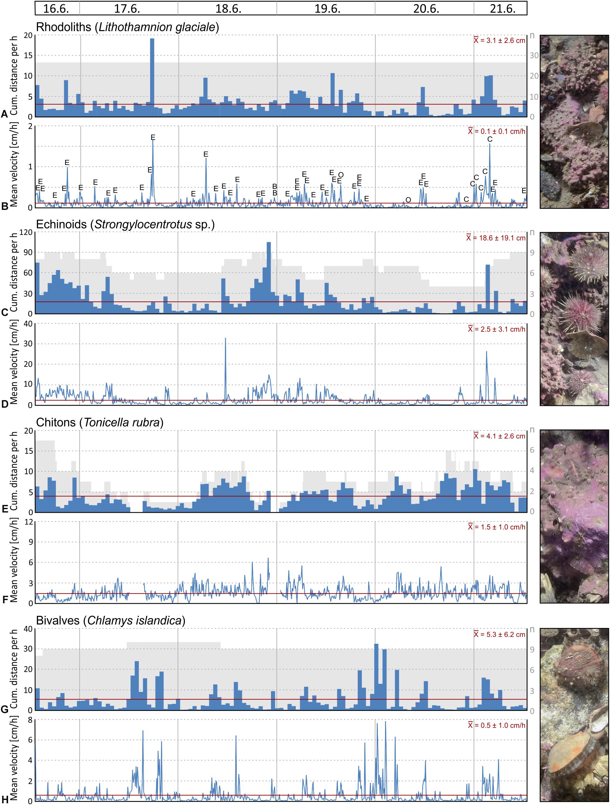
Figure 15. Cumulative distance per hour, mean velocity, and number of selected macrobenthos organisms, as tracked on images of the lander’s camera system during the 6 days of deployment in Mosselbukta: rhodoliths (A,B), echinoids (C,D), chitons (E,F), and epibenthic bivalves (G,H). Abbreviations used for indicating disturbances: E, echinoid; O, ophiuroid; C, crab; B, bivalve.

The echinoid Strongylocentrotus sp. was not only identified as the main reason for dislocation of rhodoliths, but is also of relevance for the carbonate factory. With respect to its size and abundance, this species contributes considerably on the one hand to the carbonate production, while on the other hand it also acts as a grazing agent and, therefore, contributes to carbonate bioerosion. In total 29 echinoids were tracked, ranging from juveniles of only 1.5 cm in diameter to large specimens of up to 5.4 cm in size. The mean size was 3.6 ± 1.1 cm. There were 4–9 individuals (mean = 6.8 ± 1.5) in the field of view at all times (Figure 15C and Supplementary Video S2 for tagged video file), translating to a density of 8–18 individuals (mean = 13.8 ± 3.1) per square metre. Most of the individual echinoids showed an alternating behavioural pattern of extended times hiding next to or buried below rhodoliths or small rocks, and times of travel across the rhodolith bed, carrying shell fragments or other mid-sized sediment particles along for masking. Other individuals hardly moved at all. As a result, the cumulative distance travelled by each of the 29 tracked echinoids varied greatly from only 9.5 to 305.6 cm, with a mean of 76.3 ± 65.7 cm. The cumulative distance travelled (and partly grazed) by all recorded echinoids during the 119 h of observation amounts to 2,212 cm. The synchronicity of this alternating activity pattern appears low and the mean cumulative distance travelled per hour (18.6 ± 19.1 cm; Figure 15C) as well as the mean velocity of movement (2.5 ± 3.1 cm/h; Figure 15D), thus, fluctuated irregularly over the course of the 6 days observation period. Overall, the mobility of the tracked echinoids was higher than average during the first, third, and fourth day, and below average during the second and fifth day of observation, thus coinciding with the degree of dislocation of the rhodoliths (see above).

Another grazing epibenthos species of relevance both for carbonate production and bioerosion is the chiton Tonicella rubra. Owing to its comparatively small size, this chiton was more difficult to track and often disappeared between the rhodoliths or boulders. Also, tracking of chitons on moving objects was unfeasible so that only tracks on stable objects were recorded. This resulted in 49 tracks, some of which potentially relate to the same individual chiton, and comprises juveniles of as small as 0.4 cm as well as large specimens of 2.3 cm in length. The mean length was found at 1.5 ± 0.4 cm. The number of tracked individuals ranged between none and 7 individuals (mean = 2.9 ± 1.6), equating to a density of 0 to 14 (mean = 5.9 ± 3.2) per square metre (Figure 15E and Supplementary Video S3 for tagged video file). Individuals were observed to either rest at one spot for extended periods of time, or browsing the substrate, thereby often rotating sideways and back and forth during grazing activity. The well-armoured individuals appeared fairly insensitive to disturbance by other epibenthos. The mean cumulative distance of dislocation per hour (4.1 ± 2.6 cm; Figure 15E) fluctuated irregularly, mainly as a result of the varying number of tracked individuals. The mean velocity (1.5 ± 1.0 cm/h; Figure 15F) fluctuated without marked peaks. The tracks browsed by the chitons were one order of magnitude shorter than that of the echinoids, and the cumulative length of all tracks amounts to only 482 cm with the longest individual track measuring 38 cm.

Finally, 10 individuals of the large clam Chlamys islandica, one of the main carbonate producers in the Svalbard rhodolith beds, were tracked. All specimens were mature and measured 4.6–7.2 cm in length from the umbo to the margin, and the mean length was 5.5 ± 0.7 cm. They are semi-mobile, with 8 specimens permanently in the field of view and only 2 specimens entering the scene during the observation period (Figure 15G and Supplementary Video S4 for tagged video file). The mean number of tracked specimens of 9.2 ± 0.4 translates to a density of 18.7 ± 0.9 individuals per square metre. While some of the individuals did not leave their site and only showed small changes in their orientation, others were very active, with frequent rotations and relocations, summing up to 153 cm in case of one of the individuals. The cumulative distance moved by all 10 individuals amounts to 626 cm, representing a mean of 5.3 ± 6.2 cm (Figure 15G), corresponding to a mean velocity of 0.5 ± 1.0 cm/h (Figure 15H). In most cases there was no recognisable reason for dislocation, but a number of events were attributable to either echinoids or large crustaceans.

Conclusions

Environmental data from repeated CTD profiling and an autonomous temperature/salinity logger on a long-term settlement platform, complemented by short-term deployments of a lander, identifies the involved water masses as follows: In the early summer, Mosselbukta is characterised by Polar Surface Water (PSW) and Atlantic Water (AW) in shallow waters and MAW from the Arctic Ocean at depth. At the rhodolith beds at ∼50 m water depth, short-term disturbances due to upwelling during storm events and seasonal fluctuations in the influence of the West and East Spitsbergen currents lead to a varying exposure to these three water masses. Relatively warm (∼5°C) AW in the summer months cools down during the polar night, forming MAW, and drops below the freezing point during the late winter months with sea ice cover, showing a PSW signature. In the summer, surface waters at Bjørnøy-Banken were in average colder and less saline, representing PSW from the Barents Sea, with some influence by warmer AW west of the Polar Front.

Short-term fluctuations logged by the lander at 46 m water depth at both study sites portrays a tidal range of 1 m maximum, temperature fluctuations less than 1°C, full marine salinities with fluctuations less than 0.2 units, and a range in pH from 8.2 to 8.4 (NBS scale). Levels of photosynthetically active radiation (PAR) were surprisingly low, with only few excursions above the detection limit in Mosselbukta, reaching a maximum of only 4.5 μmol/s^∗m². Accordingly, the observed turbidity was considerable, especially at Bjørnøy-Banken, where levels peaked during ebbing tide.

At both study sites, dissolved inorganic nutrients (nitrate, nitrite, phosphate) were found depleted with an overall increase in concentration and N:P ratios toward deeper waters. Together with elevated ammonium levels, this is taken to reflect a recycling system that keeps fuelling primary production (promoting the food chain for zooplankton and filter-feeding epibenthos feeding upon it) after the spring bloom (at the time of the MSM55 cruise in June 2016). This interpretation is in good accordance to elevated oxygen levels and considerably reduced carbon dioxide concentrations (pCO₂) of in average only half the expected equilibrium values, which is understood as an effect of limited air-sea gas exchange during seasonal ice cover in combination with a boost in community photosynthesis during the phytoplankton bloom. In the case of Mosselbukta, this effect is further enhanced by the onset of rhodophyte photosynthesis in the rhodolith beds during the polar day upon retreat of sea-ice. Constant total alkalinity (TA), constant or decreasing DIC, and an increase in pCO₂ levels with depth, are mirrored by carbonate saturation states and pH values decreasing with depth, but remain well within the range of oversaturation, thus suggesting little effect of physicochemical carbonate dissolution on the marine calcifiers. Hence, adverse effects of ocean acidification predicted for Arctic calcifiers are expected to be buffered to some extent by the marked annual drop in pCO₂ during the phase of seasonal sea-ice cover and spring plankton bloom. However, this should not be taken as an all-clear signal, since this positive effect will dwindle if the degree of seasonal sea-ice formation continues to decline at the present rate.

Seawater stable carbon isotope signals from both sites show an overall decrease in δ¹³C_DIC and δ¹³C_as (adjusted for phosphate) from surface to depth, and a close relationship of δ¹³C_DIC with phosphate concentrations, providing further consistency in the interpretation presented above. Seawater stable oxygen isotope ratios (δ¹⁸O_sw), instead, show a relation to salinity and in Mosselbukta describe a first order mixing line resulting from meltwater influx. Together with published data, a relatively robust, Svalbard system-specific δ¹⁸O_sw – salinity relationship is evident. All of these observed effects and bathymetrical trends are more pronounced in Mosselbukta, primarily owing to the high abundance and photosynthetic activity of the rhodophyte algae, when compared to Bjørnøy-Banken, where a strong hydrodynamic regime is promoting water column homogenisation.

Among the 25 macrobenthos taxa recorded by the lander’s camera system, 72% were crustaceans, echinoderms, and molluscs, and all but three species were calcifiers contributing to the carbonate production in the Svalbard carbonate factories. Diversity was found to be considerably higher in Mosselbukta (21 taxa) compared to Bjørnøy-Banken (8 taxa). This is interpreted as an enhanced biodiversity in the 3D habitat structured by the bioengineering crustose alga Lithothamnion glaciale in the rhodolith beds. Filter-feeding activity of balanids, serpulids, and bivalves did reveal group-specific but no common activity patterns of the densely populated Mosselbukta macrobenthos. Disturbance events by other individuals were common (in contrast to abiotic factors) with hermit crabs representing the primary cause. At Bjørnøy-Banken, holothuroid feeding activity revealed an increasing filtering rate during high tides, as reflected also in a statistically significant relation to turbidity and tidal cycle.

Motion tracking of 28 L. glaciale rhodoliths revealed a high frequency of dislocation with a mean of 13.3 cm during the 6 days of observation. Intriguingly, none of the dislocations was caused by abiotic factors but instead are attributable to the activity of other benthic organisms, in particular echinoids ploughing below or moving over the rhodoliths (88.8%), as well as large crustaceans (11.6%). Accordingly, the echinoid Strongylocentrotus sp. was identified as the most abundant component of the associated fauna, with a mean of 13.8 individuals per square metre, hence considerably contributing both to carbonate production and to grazing bioerosion. The 29 logged echinoids in the field of view travelled a cumulative distance of 2,212 cm at a mean velocity of 2.5 cm/h. The chiton Tonicella rubra was the second grazer species of relevance for carbonate production and bioerosion, travelling a cumulative 482 cm at a mean velocity of 1.5 cm/h. Another abundant calcifier is the large clam Chlamys islandica that has a semi-sessile behaviour but the cumulative distance of active dislocations of the 10 logged individuals nevertheless sums up to 626 cm. No synchronicity in the activity pattern, neither within not between the observed species, was observed.

In summary, the results of this multidisciplinary characterisation of two contrasting polar carbonate factories portray a high degree of seasonal as well as short-term dynamics in environmental conditions that support distinctly different communities and biodiversity patterns in the dominant calcifying macrobenthos. It remains paramount to further investigate the ecophysiological response of L. glaciale and other calcifiers in polar carbonate factories to the strong seasonal fluctuations in the carbonate system and other environmental variables to better understand the impact of the ongoing global change on these ecosystems.

Author Contributions

MW planned, proposed, and led the MSM55 research cruise to Svalbard, in which all authors, except for PL, participated. AR and JR performed the CTDs and together with JB took care of taking water samples. JB organised, processed and interpreted the dissolved inorganic nutrient and carbonate system analyses, while JR organised, processed and interpreted the stable isotope analyses. AR evaluated the CTD data and provided the interpretation of the water masses. MW designed, built, and employed the settlement platform, he designed (with support of PL) and employed the SaM lander, and he processed and analysed the resulting environmental data and seafloor images, except for the macrobenthos diversity and feeding activity analyses, that were carried out by HN. All authors contributed to discussion and writing of the manuscript.

Funding

The MSM55 cruise was funded by the Deutsche Forschungsgemeinschaft in concert with the Leitstelle Deutsche Forschungsschiffe. Additional financial support was provided by GEOMAR and SENCKENBERG, the two principal research institutions involved, as well as by Anneleen Foubert (Université de Fribourg), who partially funded the stable isotope analyses (SNF project ‘4D-Diagenesis@Mound’ # 200021_149247). The publication of this article was funded by the Open Access Fund of the Leibniz Association.

Conflict of Interest

The authors declare that the research was conducted in the absence of any commercial or financial relationships that could be construed as a potential conflict of interest.

Acknowledgments

Armin Form (GEOMAR, Kiel) and André Freiwald (SENCKENBERG am Meer, Wilhelmshaven) are highly acknowledged for co-proposing the MSM55 cruise together with the principal author of this contribution. Karen Hissmann, Jürgen Schauer and Peter Striewsky, alias ‘The JAGO team’ (GEOMAR, Kiel), are acknowledged for their excellent support, and Eduard Fabrizius (GEOMAR, Kiel) is thanked for assisting with the integration of the Ocean Imaging System into the SaM Lander. The SENCKENBERG technicians Maik Wilsenack and Ralf Kuhlmann are thanked for their fruitful collaboration in designing, building, and employing the SaM Lander. GEOMAR technician Kerstin Nachtigall is thanked for support in water sample analyses. Research permits were issued by The Norwegian Petroleum Directorate (Ref #: OD 15/1045-/HeHa), The Directorate of Fisheries (Ref #: 15/14719) and the Norwegian National Joint Headquarters, and we thank the Deutsche Botschaft Oslo for the help in acquiring those permits. We thank Briese Research, the Senatskommission für Ozeanographie, and the Leitstelle Deutsche Forschungsschiffe for their logistic support. We are indebted to captain Ralf Schmidt and the entire crew of RV Maria S. Merian for their superb commitment and great hospitality – the foundation for making this cruise a scientific success. Last but not least, we thank the two reviewers of this manuscript for providing valuable comments and suggestions.

Supplementary Material

The Supplementary Material for this article can be found online at: https://www.frontiersin.org/articles/10.3389/fmars.2019.00667/full#supplementary-material

TABLE S1 | Star Oddi DST CT miniature logger raw data of long-term deployment (August 2016 - November 2017) in Mosselbukta; plotted in Figures 3A,B.

TABLE S2 | Lander RBRconcerto logger raw data of deployments in Mosselbukta and Bj rn y-Banken, used for graphs in Figures 5, 7B–D.

TABLE S3 | MSM55 weather station raw data (extracted from DShip system), used for graphs in Figure 6.

TABLE S4 | MSM55 CTD raw data for graphs in Figures 7A,C, 8, 9, 10E.

TABLE S5 | MSM55 water sample analyses (nutrient regime, carbonate system, stable isotopes), used for Tables 2–4 and for graphs in Figure 10.

VIDEO S1 | Motion tracking of Mosselbukta rhodoliths (video file; mp4; uncompressed video files and the high-resolution image stack are available from the corresponding author upon request).

VIDEO S2 | Motion tracking of Mosselbukta echinoids (video file; mp4).

VIDEO S3 | Motion tracking of Mosselbukta chitons (video file; mp4).

VIDEO S4 | Motion tracking of Mosselbukta bivalves (video file; mp4).

Footnotes

1. ^ https://planetcalc.com/300
2. ^ http://polarview.met.no
3. ^ http://odv.awi.de
4. ^ http://nsidc.org
5. ^ http://data.giss.nasa.gov/o18data

References

AMAP (2018). AMAP assessment 2018: Arctic Ocean Acidification. Tromsø: Arctic Monitoring and Assessment Programme, 187.

Google Scholar

Andruleit, H., Freiwald, A., and Schäfer, P. (1996). Bioclastic carbonate sediments on the southwestern Svalbard Shelf. Mar. Geol. 134, 163–182. doi: 10.1016/0025-3227(96)00044-8

CrossRef Full Text | Google Scholar

Barbera, C., Bordehore, C., Borg, J. A., Glémarec, M., Grall, J., Hall-Spencer, J. M., et al. (2003). Conservation and management of northeast Atlantic and Mediterranean maerl beds. Mar. Freshwater. Ecosys. 13, S65–S76.

Google Scholar

Barnes, D. K. A., and Tarling, G. A. (2017). Polar oceans in a changing climate. Curr. Biol. 27, R431–R510. doi: 10.1016/j.cub.2017.01.045

PubMed Abstract | CrossRef Full Text | Google Scholar

Basso, D. (2012). Carbonate production by calcareous red algae and global change. Geodiversitas 34, 13–33. doi: 10.5252/g2012n1a2

CrossRef Full Text | Google Scholar

Basso, D., and Granier, B. (2012). Calcareous algae in changing environments. Geodiversitas 34, 5–11. doi: 10.5252/g2012n1a1

CrossRef Full Text | Google Scholar

Bauch, D., Erlenkeuser, H., and Andersen, N. (2005). Water mass processes on Arctic shelves as revealed from δ¹⁸O of H₂O. Global Planet. Change 48, 165–174. doi: 10.1016/j.gloplacha.2004.12.011

CrossRef Full Text | Google Scholar

Bauch, D., Polyak, L., and Ortiz, J. D. (2015). A baseline for the vertical distribution of the stable carbon isotopes of dissolved inorganic carbon (δ¹³C_DIC) in the Arctic Ocean. Arktos 1:15.

Google Scholar

Bauch, D., Rutgers van der Loeff, M., Andersen, D., Torres-Valdes, S., Bakker, K., and Abrahamsen, E. P. (2011). Origin of freshwater and Polynya water in the Arctic Ocean halocline in summer 2007. Prog. Oceanogr. 91, 482–495. doi: 10.1016/j.pocean.2011.07.017

CrossRef Full Text | Google Scholar

Bauch, D., Schlosser, P., and Fairbanks, R. F. (1995). Freshwater balance and the sources of deep and bottom waters in the Arctic Ocean inferred from the distribution of H₂¹⁸O. Prog. Oceanogr. 35, 53–80. doi: 10.1016/0079-6611(95)00005-2

CrossRef Full Text | Google Scholar

Bedard, P., Hillaire-Marcel, C., and Page, C. (1981). ¹⁸O modelling of freshwater inputs in Baffin Bay and Canadian Arctic coastal waters. Nature 293, 287–289. doi: 10.1038/293287a0

CrossRef Full Text | Google Scholar

Brand, W. A., Coplen, T. B., Vogl, J., Rosner, M., and Prohaska, T. (2014). Assessment of international reference materials for isotope-ratio analysis (IUPAC Technical Report). Pure Appl. Chem. 86, 263–467.

Google Scholar

Broecker, W. S., and Maier-Reimer, E. (1992). The influence of air and sea exchange on the carbon isotope distribution in the sea. Glob. Biogeochem. Cycles 6, 315–320. doi: 10.1029/92gb01672

CrossRef Full Text | Google Scholar

Büdenbender, J., Riebesell, U., and Form, A. (2011). Calcification of the Arctic coralline red algae Lithothamnion glaciale in response to elevated CO₂. Mar. Ecol. Prog. Ser. 441, 79–87. doi: 10.3354/meps09405

CrossRef Full Text | Google Scholar

CAFF (2017). State of the Arctic Marine Biodiversity Report. Akureyri: Conservation of Arctic Flora and Fauna International Secretariat.

Google Scholar

Cooper, L. W., McClelland, J. W., Holmes, R. M., Raymond, P. A., Gibson, J. J., Guay, C. K., et al. (2008). Flow-weighted values of runoff tracers (δ¹⁸O, DOC, Ba, alkalinity) from the six largest Arctic rivers. Geophys. Res. Lett. 35:L18606.

Google Scholar

Cottier, F., Tverberg, V., Inall, M., Svendsen, H., Nilsen, F., and Griffiths, C. (2005). Water mass modification in an Arctic fjord through cross-shelf exchange: the seasonal hydrography of Kongsfjorden, Svalbard. J. Geophys. Res. 110:C21005.

Google Scholar

Davoult, D., and Gounin, F. (1995). Suspension-feeding activity of a dense Ophiothrix fragilis (Abildgaard) population at the water-sediment interface: time coupling of food availability and feeding behaviour of the species. Est. Coast. Shelf Sci. 41, 567–577. doi: 10.1016/0272-7714(95)90027-6

CrossRef Full Text | Google Scholar

Diaz-Pulido, G., Anthony, K. R. N., Kline, D. I., Dove, S., and Hoegh-Guldberg, O. (2012). Interactions between ocean acidification and warming on the mortality and dissolution of coralline algae. J. Phycol. 48, 32–39. doi: 10.1111/j.1529-8817.2011.01084.x

PubMed Abstract | CrossRef Full Text | Google Scholar

Dickson, A. G., Afghan, J. D., and Anderson, G. C. (2003). Reference materials for oceanic CO₂ analysis: a method for the certification of total alkalinity. Mar. Chem. 80, 185–197. doi: 10.1016/s0304-4203(02)00133-0

CrossRef Full Text | Google Scholar

Dickson, A. G., and Millero, F. J. (1987). A comparison of the equilibrium constants for the dissociation of carbonic acid in seawater media. Deep Sea Res. 34, 1733–1743. doi: 10.1016/0198-0149(87)90021-5

CrossRef Full Text | Google Scholar

Dickson, A. G., Sabine, C. L., and Christian, J. R. (eds). (2007). Guide to Best Practices for Ocean CO₂ Measurements. IOCC Report No. 8. Sidney, BC: PICES Special Publication.

Google Scholar

Doney, S. C., Fabry, V. J., Feely, R. A., and Kleypas, J. A. (2009). Ocean acidification: the other CO₂ problem. Ann. Rev. Mar. Sci. 1, 169–192.

PubMed Abstract | Google Scholar

Foster, M. S. (2001). Rhodolites: between rocks and soft places. J. Phycol. 37, 659–667. doi: 10.1046/j.1529-8817.2001.00195.x

CrossRef Full Text | Google Scholar

Freiwald, A. (1998). Modern nearshore cold-temperate calcareous sediments in the Troms District, northern Norway. J. Sediment. Res. A 68, 763–776. doi: 10.2110/jsr.68.763

CrossRef Full Text | Google Scholar

Friedrich, H., Houssais, M.-N., Quadfasel, D., and Rudels, B. (1995). “On Fram Strait water masses,” in Proceedings of the Extended Abstract, Nordic Seas Symposium, Hamburg, 69–72.

Google Scholar

Gerlach, S. A., and Graf, G. (1991). Europäisches Nordmeer, Reise Nr. 13 vom 6. Juli – 24. August 1990. METEOR-Berichte; 91-92. Hamburg: Leitstelle METEOR, doi: 10.2312/CR_M13

CrossRef Full Text | Google Scholar

Grebmeier, J. M., and Barry, J. P. (1991). The influence of oceanographic processes on pelagic-benthic coupling in polar regions: a benthic perspective. J. Mar. Syst. 2, 495–518. doi: 10.1016/0924-7963(91)90049-z

CrossRef Full Text | Google Scholar

Halfar, J., Adey, W. H., Kronz, A., Hetzinger, S., Edinger, E., and Fitzhugh, W. W. (2013). Arctic sea-ice decline archived by multicentury annual-resolution record from crustose coralline algal proxy. Proc. Natl. Acad. Sci. U.S.A. 110, 19737–19741. doi: 10.1073/pnas.1313775110

PubMed Abstract | CrossRef Full Text | Google Scholar

Hall-Spencer, J. M., Rodolfo-Metalpa, R., Martin, S., Ransome, E., Fine, M., Turner, S. M., et al. (2008). Volcanic carbon dioxide vents show ecosystem effects of ocean acidification. Nature 454, 96–99. doi: 10.1038/nature07051

PubMed Abstract | CrossRef Full Text | Google Scholar

Hamel, J. F., and Mercier, A. (1998). Diet and feeding behaviour of the sea cucumber Cucumaria frondosa in the St. Lawrence estuary, eastern Canada. Can. J. Zool. 76, 1194–1198. doi: 10.1139/z98-040

CrossRef Full Text | Google Scholar

Hansen, H. P., and Koroleff, F. (1999). “Determination of nutrients,” in Methods of Seawater Analysis, eds K. Grasshoff, K. Kremling, and M. Ehrhardt (Weinheim: Verlag Chemie), 159–228. doi: 10.1002/9783527613984.ch10

CrossRef Full Text | Google Scholar

Harris, C. L., Plueddemann, A. J., and Gawarkiewicz, G. G. (1998). Water mass distribution and polar front structure in the western Barents Sea. J. Geophys. Res. 103, 2905–2917. doi: 10.1029/97jc02790

CrossRef Full Text | Google Scholar

Henrich, R., Freiwald, A., Betzler, C. B., Bader, B., Schäfer, P., Samtleben, C., et al. (1995). Controls on modern carbonate sedimentation on warm-temperate to Arctic coasts, shelves and seamounts in the northern hemisphere: implications for fossil counterparts. Facies 32, 71–108. doi: 10.1007/bf02536865

CrossRef Full Text | Google Scholar

Henrich, R., Freiwald, A., Bickert, T., and Schäfer, P. (1997). “Evolution of an Arctic open-shelf carbonate platform, Spitsbergen Bank (Barents Sea),” in Cool-water carbonates, Vol. 56, eds N. P. James and J. A. D. Clarke (Broken Arrow, OK: SEPM Special Publication), 163–181. doi: 10.2110/pec.97.56.0163

CrossRef Full Text | Google Scholar

Henrich, R., Freiwald, A., Wehrmann, A., Schäfer, P., Samtleben, C., and Zankl, H. (1996). Nordic cold-water carbonates: occurrences and controls. Göttinger Arb. Geol. Paläontol., Sb 2, 35–52.

Google Scholar

Hetzinger, S., Halfar, J., Zajacz, Z., and Wisshak, M. (2019). Early start of 20th-century Arctic sea-ice decline recorded in Svalbard coralline algae. Geology 47, 963–967. doi: 10.1130/g46507.1

CrossRef Full Text | Google Scholar

Hodal, H., Falk-Petersen, S., Hop, H., Kristiansen, S., and Reigstad, M. (2012). Spring bloom dynamics in Kongsfjorden, Svalbard: nutrients, phytoplankton, protozoans and primary production. Polar Biol. 35, 191–203. doi: 10.1007/s00300-011-1053-7

CrossRef Full Text | Google Scholar

Hop, H., Pearson, T., Hegseth, E. N., Kovacs, K., Wiencke, C., Kwasniewski, S., et al. (2002). The ecosystem of Kongsfjorden, Svalbard. Polar Res. 21, 167–208.

Google Scholar

Islam, F., DeGrandpre, M., Beatty, C., Krishfield, R., and Toole, J. (2016). Gas exchange of CO₂ and O₂ in partially ice covered regions of the Arctic Ocean investigated using in situ sensors. IOP Conf. Ser. Earth Environ. Sci. 35:7.

Google Scholar

Iversen, K. R., and Seuthe, L. (2011). Seasonal microbial processes in a high-latitude fjord (Kongsfjorden, Svalbard): I. Heterotrophic bacteria, picoplankton and nanoflagellates. Polar Biol. 34, 731–749. doi: 10.1007/s00300-010-0929-2

CrossRef Full Text | Google Scholar

James, N. P., and Clarke, J. A. D. (1997). Cool-Water Carbonates. Broken Arrow, OK: SEPM.

Google Scholar

Johannessen, O. M., and Foster, L. A. (1978). A note on the topographically controlled oceanic Polar Front in the Barents Sea. J. Geophys. Res. 83, 4567–4571.

Google Scholar

Jørgensen, C. B. (1966). Biology of Suspension Feeding. Oxford: Pergamon Press.

Google Scholar

Kerr, R. A. (2012). Ice-free Arctic Sea may be years, not decades away. Science 337:1591. doi: 10.1126/science.337.6102.1591

PubMed Abstract | CrossRef Full Text | Google Scholar

Kjellman, F. R. (1883). The Algae of the Arctic Sea. Stockholm: Kongl. Boktryckeriet.

Google Scholar

Kroopnick, P. M. (1985). The distribution of ¹³C on ΣCO₂ in the world oceans. Deep Sea Res. A 32, 57–84. doi: 10.1016/0198-0149(85)90017-2

CrossRef Full Text | Google Scholar

Kuffner, I. B., Andersson, A. J., Jokiel, P. L., Rodgers, K. S., and Mackenzie, F. T. (2007). Decreased abundance of crustose coralline algae due to ocean acidification. Nat. Geosci. 1, 114–117. doi: 10.1038/ngeo100

CrossRef Full Text | Google Scholar

Kuklinski, P., and Barnes, D. K. A. (2005). Microhabitat diversity of Svalbard Bryozoa. J. Nat. Hist. 39, 539–554. doi: 10.1080/00222930400001350

CrossRef Full Text | Google Scholar

Kuklinski, P., Barnes, D. K. A., and Taylor, P. D. (2006). Latitudinal patterns of diversity and abundance in North Atlantic intertidal boulder-fields. Mar. Biol. 149, 1577–1583. doi: 10.1007/s00227-006-0311-7

CrossRef Full Text | Google Scholar

Leonard, A. B. (1989). Functional response in Antedon mediterranea (Lamarck) (Echinodermata: Crinoidea): the interaction of prey concentration and current velocity on a passive suspension-feeder. J. Exp. Mar. Biol. Ecol. 127, 81–103. doi: 10.1016/0022-0981(89)90210-4

CrossRef Full Text | Google Scholar

Lherminier, P., Meincke, J., Freiwald, A., and Schauer, U. (eds) (2009). Circulation and Ecosystems in the Subpolar and Polar North Atlantic, MARIA S. MERIAN-Berichte 09-1 Cruise No. 2. Hamburg: Institut für Meereskunde, 174.

Google Scholar

Lynch-Stieglitz, J., Stocker, T. F., Broecker, W., and Fairbanks, R. G. (1995). The influence of air–sea exchange on the isotopic composition of oceanic carbon: observation and modeling. Glob. Biogeochem. Cycles 9, 653–665. doi: 10.1029/95gb02574

CrossRef Full Text | Google Scholar

MacLachlan, S. E., Cottier, F. R., Austin, W. E. N., and Howe, J. A. (2007). The salinity: δ¹⁸O water relationship in Kongsfjorden, western Spitsbergen. Polar Res. 26, 160–167. doi: 10.1111/j.1751-8369.2007.00016.x

CrossRef Full Text | Google Scholar

McConnico, L. A., Foster, M. S., Steller, D. L., and Riosmena-Rodríguez, R. (2014). Population biology of a long-lived rhodolith: the consequences of becoming old and large. Mar. Ecol. Prog. Ser. 504, 109–118. doi: 10.3354/meps10780

CrossRef Full Text | Google Scholar

Mehrbach, C., Culberso, C. H., Hawley, J. E., and Pytkowic, R. M. (1973). Measurement of apparent dissociation constants of carbonic acid in seawater at atmospheric pressure. Limnol. Oceanogr. 18, 897–907. doi: 10.4319/lo.1973.18.6.0897

CrossRef Full Text | Google Scholar

Mikalsen, G., and Sejrup, H. P. (2000). Oxygen isotope composition of fjord and river water in the Sognefjorden drainage area, western Norway. Implications for paleoclimate studies. Estuar. Coast. Mar. Sci. 50, 441–448. doi: 10.1006/ecss.1999.0581

CrossRef Full Text | Google Scholar

Morse, J. W., Andersson, A. J., and Mackenzie, F. T. (2006). Initial responses of carbonate-rich shelf sediments to rising atmospheric pCO₂ and ocean acidification: role of high Mg calcites. Geochim. Cosmochim. Acta 70, 5814–5830. doi: 10.1016/j.gca.2006.08.017

CrossRef Full Text | Google Scholar

Orr, J. C., Fabry, V. J., Aumont, O., Bopp, L., Doney, S. C., Feely, R. A., et al. (2005). Anthropogenic ocean acidification over the twenty-first century and its impact on calcifying organisms. Nature 437, 681–686. doi: 10.1038/nature04095

PubMed Abstract | CrossRef Full Text | Google Scholar

Pedley, M., and Carannante, G. (2006). Cool-water carbonate ramps: a review. Geol. Soc. Lond. Spec. Publ. 255, 1–9. doi: 10.1144/gsl.sp.2006.255.01.01

CrossRef Full Text | Google Scholar

Pfannkuche, O., Duinker, J. C., Graf, G., Henrich, R., Thiel, H., and Zeitschel, B. (1993). Nordatlantik 1992, Reise Nr. 21, 16. März – 31. August 1992. Meteor-Berichte; 93-4. Hamburg: Leitstelle METEOR, 1–281.

PubMed Abstract | Google Scholar

Piepenburg, D. (2005). Recent research on Arctic benthos: common notions need to be revised. Polar Biol. 28, 733–755. doi: 10.1007/s00300-005-0013-5

CrossRef Full Text | Google Scholar

Piepenburg, D., Archambault, P., Ambrose, W. G., Blanchard, A. L., Bluhm, B. A., Carroll, M. L., et al. (2011). Towards a pan-Arctic inventory of the species diversity of the macro- and megabenthic fauna of the Arctic shelf seas. Mar. Biodiv. 41, 51–70. doi: 10.1007/s12526-010-0059-7

CrossRef Full Text | Google Scholar

Piepenburg, D., Chernova, N. V., von Dorrien, C. F., Gutt, J., Neyelov, A. V., Rachor, E., et al. (1996). Megabenthic communities in the waters around Svalbard. Pol. Biol. 16, 431–446. doi: 10.1007/bf02390425

CrossRef Full Text | Google Scholar

Pierrot, D., Lewis, E., and Wallace, D. W. R. (2006). MS Excel program developed for CO₂ system calculations. ORNL/CDIAC-105a. Oak Ridge, TN: Carbon Dioxide Information Analysis Centre.

Google Scholar

Raddatz, J., Liebetrau, V., Trotter, J., Rüggeberg, A., Flögel, S., Eisenhauer, A., et al. (2016). Environmental constraints on Holocene cold-water coral reef growth off Norway: insights from a multiproxy approach. Paleoceanography 31, 1350–1367. doi: 10.1002/2016pa002974

CrossRef Full Text | Google Scholar

Rudels, B., Bjørk, G., Muench, R. D., and Schauer, U. (1999). Double-diffusive layering in the Eurasian Basin of the Arctic Ocean. J. Mar. Syst. 21, 3–27. doi: 10.1016/s0924-7963(99)00003-2

CrossRef Full Text | Google Scholar

Rudels, B., Meyer, R., Fahrbach, E., Ivanov, V. V., Èsterhus, S., Quadfasel, D., et al. (2000). Water mass distribution in Fram Strait and over the Yermak Plateau in summer 1997. Ann. Geophys. 18, 687–705. doi: 10.1007/s00585-000-0687-5

CrossRef Full Text | Google Scholar

Sahade, R., Stellfeldt, A., Tatián, M., and Laudien, J. (2004). Macro-Epibenthic Communities and Diversity of Arctic Kongsforden, Svalbard, in Relation To Depth And Substrate. The Coastal Ecosystem of Kongsfjorden, Svalbard: Synopsis of Biological Research Performed at the Koldewey Station in the years 1991-2003. Bremerhaven: Alfred-Wegener-Institut für Polar-und Meeresforschung.

Google Scholar

Sanz-Martín, M., Chierici, M., Mesa, E., Carrillo-de-Albornoz, P., Delgado-Huertas, A., Agustí, S., et al. (2018). Episodic Arctic CO₂ limitation in the West Svalbard Shelf. Front. Mar. Sci. 5:221. doi: 10.3389/fmars.2018.00221

CrossRef Full Text | Google Scholar

Schlager, W. (2000). “Sedimentation rates and growth potential of tropical, cool-water and mud-mound carbonate factories,” in Carbonate Platform Systems, eds E. Insalaco, P. W. Skelton, and T. J. Palmer (London: Geological Society), 217–227. doi: 10.1144/gsl.sp.2000.178.01.14

CrossRef Full Text | Google Scholar

Schlager, W. (2005). Carbonate sedimentology and sequence stratigraphy. Soc. Sediment. Geol. 8:200. doi: 10.2110/csp.05.08

CrossRef Full Text | Google Scholar

Schmidt, G. A., Bigg, G. R., and Rohling, E. J. (1999). Global Seawater Oxygen-18 Database-v1.21. Available at: http://data.giss.nasa.gov/o18data/

Google Scholar

Schönberg, C. H. L., Fang, J. K. H., Carreiro-Silva, M., Tribollet, A., and Wisshak, M. (2017). Bioerosion: the other ocean acidification problem. ICES J. Mar. Sci. 74, 895–925. doi: 10.1098/rstb.2012.0442

PubMed Abstract | CrossRef Full Text | Google Scholar

Schulz, K. G., Bellerby, R. G. J., Brussard, C. P. D., Büdenbender, J., Czerny, J., Engel, A., et al. (2013). Temporal biomass dynamics of an Arctic plankton bloom in response to increasing levels of atmospheric carbon dioxide. Biogeosciences 10, 161–180. doi: 10.5194/bg-10-161-2013

CrossRef Full Text | Google Scholar

Scoffin, T. P. (1988). The environments of production and deposition of calcareous sediments on the shelf west of Scotland. Sediment. Geol. 60, 107–124. doi: 10.1016/0037-0738(88)90113-3

CrossRef Full Text | Google Scholar

Singh, R., MacDonald, B. A., Lawton, P., and Thomas, M. L. (1998). Feeding response of the dendrochirote sea cucumber Cucumaria frondosa (Echinodermata: Holothuroidea) to changing food concentrations in the laboratory. Can. J. Zool. 76, 1842–1849. doi: 10.1139/cjz-76-10-1842

CrossRef Full Text | Google Scholar

Singh, R., MacDonald, B. A., Thomas, M. L., and Lawton, P. (1999). Patterns of seasonal and tidal feeding activity in the dendrochirote sea cucumber Cucumaria frondosa (Echinodermata: Holothuroidea) in the Bay of Fundy, Canada. Mar. Ecol. Progr. Ser. 187, 133–145. doi: 10.3354/meps187133

CrossRef Full Text | Google Scholar

Stein, R., Fahl, K., Gierz, P., Niessen, F., and Lohmann, G. (2017). Arctic Ocean sea ice cover during the penultimate glacial and the last interglacial. Nat. Commun. 8, 1–13. doi: 10.1038/s41467-017-00552-1

PubMed Abstract | CrossRef Full Text | Google Scholar

Suess, E., Kremling, K., and Mienert, J. (1994). Nordatlantik 1993, Cruise No. 26, 24. August – 26 November 1993. Meteor-Berichte, Vol. 94-4. Hamburg: Leitstelle METEOR, 1–256.

Google Scholar

Teichert, S. (2014). Hollow rhodoliths increase Svalbard’s shelf biodiversity. Sci. Rep. 4:6972.

Google Scholar

Teichert, S., and Freiwald, A. (2014). Polar coralline algal CaCO₃-production rates correspond to intensity and duration of the solar radiation. Biogeosciences 11, 833–842. doi: 10.5194/bg-11-833-2014

CrossRef Full Text | Google Scholar

Teichert, S., Woelkerling, W., Rüggeberg, A., Wisshak, M., Piepenburg, D., Meyerhöfer, M., et al. (2012). Rhodolith beds (Corallinales, Rhodophyta) and their physical and biological environment at 80°31’ N in Nordkappbukta (Nordaustlandet, Svalbard Archipelago, Norway). Phycologia 51, 371–390. doi: 10.2216/11-76.1

CrossRef Full Text | Google Scholar

Teichert, S., Woelkerling, W., Rüggeberg, A., Wisshak, M., Piepenburg, D., Meyerhöfer, M., et al. (2014). Arctic rhodolith beds and their environmental controls (Spitsbergen, Norway). Facies 60, 15–37. doi: 10.1007/s10347-013-0372-2

CrossRef Full Text | Google Scholar

van Geldern, R., Schulte, P., Mader, M., Baier, A., and Barth, J. A. C. (2015). Spatial and temporal variations of pCO₂, dissolved inorganic carbon and stable isotopes along a temperate karstic watercourse. Hydrol. Process. 29, 3423–3440. doi: 10.1002/hyp.10457

CrossRef Full Text | Google Scholar

Weslawski, J. M., Wlodarska-Kowalczuk, M., and Legesynzka, J. (2003). Occurrence of soft bottom macrofauna along the depth gradient in High Arctic, 79° N. Polish Pol. Res. 24, 73–88.

Google Scholar

Wiborg, K. F. (1970). Utbredelse av haneskjell (Chlamys islandica MÜLLER) på Bjørnøybankene. Fiskets Gang 43, 782–788.

Google Scholar

Wiodarska-Kowalczuk, M., Kuklijski, P., Ronowicz, M., Legeryjska, J., and Gromisz, S. (2009). Assessing species richness of macrofauna associated with macroalgae in Arctic kelp forests (Hornsund, Svalbard). Polar Biol. 32, 897–905. doi: 10.1007/s00300-009-0590-9

CrossRef Full Text | Google Scholar

Wisshak, M., Bartholomä, A., Beuck, L., Büscher, J., Form, A., Freiwald, A., et al. (2017). Habitat characteristics and carbonate cycling of macrophyte-supported polar carbonate factories (Svalbard), MARIA S. MERIAN-Berichte, Cruise No. MSM55. Bremen: DFG-Senatskommission für Ozeanographie, 58.

Google Scholar