Fine Scale Assemblage Structure of Benthic Invertebrate Megafauna on the North Pacific Seamount Mokumanamana
 Nicole B. Morgan
 Savannah Goode
 E. Brendan Roark2
  Amy R. Baco
- 1Department of Earth, Ocean and Atmospheric Science, Florida State University, Tallahassee, FL, United States
- 2Department of Geography, Texas A&M University, College Station, TX, United States
Changes in benthic megafaunal assemblage structure have been found across gradients of environmental variables for many deep-sea habitats, but patterns remain under-investigated on seamounts. To assess the extent of variability in benthic communities at the scale of within a single seamount, and to assess environmental drivers of assemblage changes, Mokumanamana, also known as Necker Island, a seamount in the Papahānaumokuākea Marine National Monument with no known history of human impacts, was surveyed. Replicate 1 km transects were conducted along depth contours at 50 m depth intervals from 200–700 m on three sides of Mokumanamana using the AUV Sentry. Megafaunal abundance and substrate parameters were obtained from 26,119 total images. The dominant megafaunal taxa were sponges, corallimorpharians, cup corals, and benthic ctenophores. Sea pens and alcyonacean octocorals were also abundant. Overall, abundance and diversity of megafauna increased with depth. Beta-diversity through species substitution with depth was very high. Beta-diversity was also high between the sides and likewise defined almost exclusively by species substitution. Crossed ANOSIM by depth and side showed community structure differed on Mokumanamana for both factors. NMDS and cluster analyses of Mokumanamana show nine assemblages that were defined by depth and reflect differences between sides of the seamount. Environmental modeling with DISTLM indicates sediment, oxygen, substrate variability and roughness, POC, and surface currents are correlated with these assemblage differences. These results suggest that microhabitats on seamounts can promote unique assemblages along depth gradients as well as on different sides of a feature, and this diversity may be easily overlooked without fine-scale sampling. These findings have implications for management and conservation of seamounts as well as future ecological studies of seamounts, as seamounts are generally sampled on much coarser spatial scales.
Introduction
Seamounts have often been treated as homogenous landscapes in ecological studies and in management efforts, but the potential heterogeneity of seamounts is beginning to emerge in the more recent literature. Rather than consistent slopes of hard substrate, seamounts often have highly irregular geology that ranges from sedimented plateaus to steep rocky cliff faces, with most grain sizes in between, all on the same feature (Levin et al., 2001; Auster et al., 2005). Large bathymetric gradients over short horizontal distances lead to large variations in temperature (Yasuhara and Danovaro, 2016) and oxygen concentrations (Levin, 2002). When those gradients are combined with surface productivity variations in the overlaying water column (Bo et al., 2011; Woolley et al., 2016) the result is a large variety of habitats over a relatively small area. Seamounts can also have higher habitat heterogeneity due to the organisms themselves as the corals and sponges that often dominate in hard substrate areas can create biogenic structures that then provide habitat for other invertebrates and fishes (e.g., Buhl-Mortensen et al., 2009).
In the general deep-sea, variation in many of these same environmental parameters has been found to be correlated with variation in megafaunal assemblage structure, abundance, and diversity. Depth is one of the more prominent parameters influencing assemblage structure (e.g., Howell et al., 2002; Quattrini et al., 2014). Other significant parameters include magnetivity and topography (Boschen et al., 2015), temperature (Mortensen and Buhl-Mortensen, 2004; Wei et al., 2010; Morgan et al., 2015), turbidity (Mamouridis et al., 2011; Brooke et al., 2017), pH (Brooke et al., 2017), oxygen (Wishner et al., 1990; Levin, 2002; De Leo et al., 2017), substrate size and type (Mortensen and Buhl-Mortensen, 2004), and stochastic processes and environmental filtering (Quattrini et al., 2016). Thus, the high habitat heterogeneity that is becoming known on many seamounts, with numerous available habitats, may then contribute to high biodiversity on seamounts. It may also lead to large variations in community structure within a single seamount, as each microhabitat on the seamount has the potential to harbor unique communities of benthic invertebrates. Indeed, several recent seamount studies support variability within and among seamount communities related to environmental variation (Baco, 2007; McClain et al., 2010; Bo et al., 2011; Williams et al., 2011; Baco and Cairns, 2012; Long and Baco, 2014; Schlacher et al., 2014; Thresher et al., 2014; McClain and Lundsten, 2015; Morgan et al., 2015; Victorero et al., 2018a; Mejia-Mercado et al., 2019).
The wide range of environmental factors, the natural variability of those factors within and between seamounts, and the concomitant variability that is likely to occur in seamount fauna, make it challenging to form inferences about the resilience of seamount fauna to anthropogenic effects. Levels of biodiversity and the assemblage structure on seamounts are an ever-growing concern for deep-sea science and ocean conservation due to the numerous anthropogenic disturbances occurring (Ramirez-Llodra et al., 2011; Pusceddu et al., 2014; Levin and Le Bris, 2015). Trawl fisheries on the high seas often target these features as they have aggregating functions for fish, acting either as cover or reproductive hot-spots (Morato and Clark, 2007). However, trawl fishing is also highly destructive to seamount ecosystems and leads to removal of biogenic structures (Althaus et al., 2009; Clark and Rowden, 2009; reviewed in Rossi, 2013; Clark et al., 2016). Clark et al. (2007) reported nearly 2.3 million tons of fish removed by trawling globally with 900,000 tons from seamounts in the North Pacific. More recent data from the Food and Agriculture Organization of the United Nations reports 14.4 million tons of fish caught by trawling globally with 2.07 million tons removed from the North Pacific alone (Victorero et al., 2018b). This translates into large areas of seamounts where any coral and sponge assemblages present, along with their associated communities of invertebrates and fishes, would have been damaged or removed by these fishing activities. Seamounts face even greater impacts from the push for mining of deep-sea substrates for semi-precious and precious metals (Halfar and Fujita, 2007; Mengerink et al., 2014; Cuvelier et al., 2018). Seamount slopes that occur from 800 to 2500 m in depth can accrue cobalt-rich manganese crusts, similar to the nodules that accrue on abyssal plains. Co-precipitates such as molybdenum, manganese, tantalum, bismuth, platinum, zirconium, tungsten, and titanium (Hein et al., 2009) are used in numerous technologies, and because land-based mine sources for these metals are confined to a few areas, terrestrial yields of these economically important resources are dwindling.
To date, most sampling methods for surveying seamounts rely on submersibles, remotely operated vehicles (ROV), towed-camera transects along the flank of the feature, or drop camera images (e.g., Stocks, 2004; Rowden et al., 2010; Vetter et al., 2010; Clark et al., 2012). Operational time constraints at any feature, especially on remote locations, limits the number and length of surveys that can be planned, often resulting in little or no replication across environmental gradients such as depth or substrate. As such, while these surveys are good for providing an ecosystem snapshot and partial species lists for a given seamount, they are not able to provide replicate sampling within features for statistical tests to compare fauna among areas on a given seamount or often even between features (Rowden et al., 2010; Sautya et al., 2011; Higgs and Attrill, 2015).
Automated Underwater Vehicle (AUV) technology, however, has advanced to where these issues of low sample coverage and replication can be rectified. AUVs can cover a greater distance than ROVs and stay on station for long periods of time (Kilgour et al., 2014). AUVs can also provide high definition imagery at a lower altitude than many towed cameras, especially on rougher and steeper topography. With more images there is a greater chance of capturing natural variability in benthic assemblages as well as multiple occurrences of rare species, and of reducing singleton samples, common issues with low replication in many ecological studies (Monk et al., 2018). New challenges arise with large numbers of images to process, but the rise in automated annotation software and machine learning have begun to make large image datasets less onerous (Schoening et al., 2016). Currently human identifications and counts, even by non-specialists, are still the most accurate method of gathering data from imagery (Matabos et al., 2017), but as computer-learning methods advance, the problem is likely to be overcome.
With the encroachment of fishing and mining onto more and more seamounts, it is important to clearly define scales of variability in faunal communities and in environmental factors on seamounts. Baseline data for variability in seamount assemblage structure are lacking due to the fact that many seamounts close enough to allow for the extended and/or repeated time on station required for thorough ecological surveys, also have a history of human activity [i.e., Northeast Pacific seamounts reviewed in Clark et al. (2007), New Zealand seamounts (Richer de Forges et al., 2000), Tasmania seamounts (Koslow et al., 2001), Mediterranean features (Bo et al., 2014), and Northeast Atlantic seamounts (Hall-Spencer et al., 2002)]. Better data on intra seamount variability are crucial for improving our understanding of seamount ecology as well as for ecological impact studies so that effects from human activity can be clearly identified and separated from natural variations in abundance or diversity. Thus, the goal of this study was to use AUV surveys for a more detailed investigation of variation within a single seamount feature than has been possible in previous seamounts studies. An unimpacted seamount was targeted to fill in gaps in baseline variability data for seamounts, to address changes in diversity and assemblage structure with depth on a single seamount, and also among sides of the same seamount feature. Additionally, environmental data were gathered to assess how observed assemblage variability may be tied to other factors. From these data we make inferences into how current approaches to sampling and managing seamounts may be affected by faunal variability.
Materials and Methods
Site Selection
Mokumanamana (Latitude 23.65°N, Longitude 164.80°W), also known as Necker Island, in the Northwest Hawaiian Islands (NWHI) was surveyed as part of a larger project surveying North Pacific seamounts, to understand impacts on deep-sea communities from trawl fisheries and to explore possible recovery times for these habitats (Baco et al., 2019; Baco et al., in review). Oceanic islands with exposed summits are included in the most recent definitions of seamounts as they are geologically identical to unexposed seamounts (Staudigel and Clague, 2010). Though there is some emergent land at Mokumanamana (Figure 1), it is a small rocky outcrop of only 0.18 km2 that does not have the features of a true island that might affect benthic assemblages [i.e., mass or channels to trap phytoplankton, freshwater run-off, increased detritus to the seafloor, or prolonged human habitation (Gilmartin and Revelante, 1974)]. Mokumanamana was selected as a target feature as it has no known history of large-scale bottom contact fishing. The seamount is also 600 km from the main Hawaiian Islands, far enough to limit human influences. Mokumanamana is an important cultural and religious site for native Hawai’ians, and has been protected legally since 1909 when Theodore Roosevelt created the Hawaiian Islands Bird Reservation. In 1988, Mokumanamana was further protected when the island specifically was added to the National Registry of Historic Palaces, and then further protected as part of the Northwestern Hawaiian Islands Coral Ecosystem Reserve in 2000. Mokumanamana continues to be protected with the establishment of the Papahānaumokuākea Marine National Monument in 2008, and further as part of the United Nations Educational, Scientific and Cultural Organization World Heritage site of Papahānaumokuākea established in 2010.
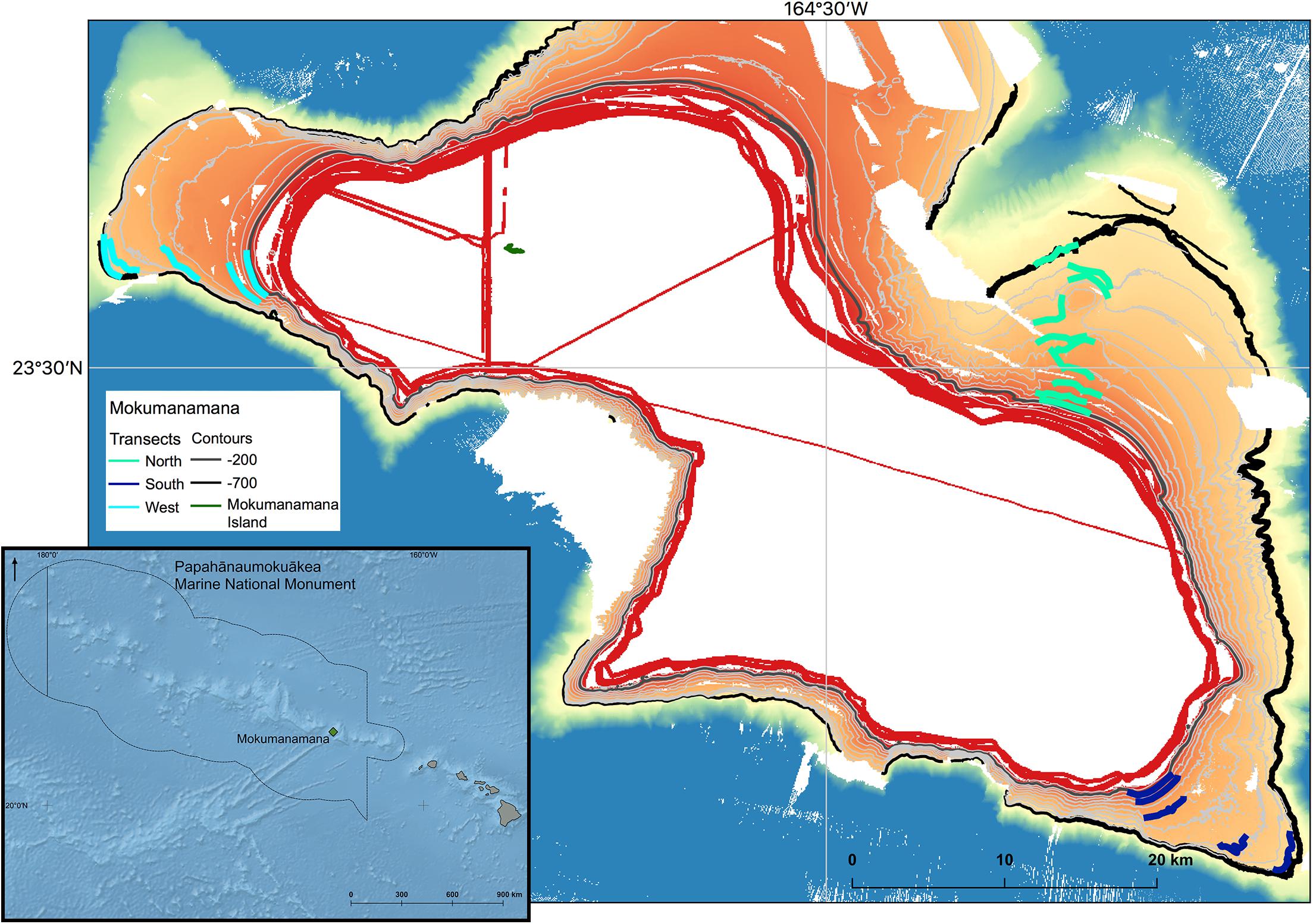
Figure 1. Bathymetry of Mokumanamana with contours from 200–700 m at 50 m intervals shown. 200 and 700 m isobars are thick contours to highlight the depth range of the study. Transects lines on each of the three sides are plotted. Inset: Overview of the location of Mokumanamana (shown in green) within the Northwestern Hawai’ian Islands and Papahânaumokuâkea Marine National Monument.
Sampling Strategy and Data Collection
In 2015 the AUV Sentry was deployed on the slope of three different sides of Mokumanamana (further referred to as “sides” to avoid confusion with the environmental parameter of slope angle) and conducted 1000 m long triplicate photographic transects at 50 m depth intervals from 200 to 700 m depth, inclusive. Locations for transects were selected based on backscatter that indicated the highest probability of hard substrate across the survey depth range, and were conducted along depth contours with a separation of at least 100 m between transects. A total of 152 km of the feature was surveyed. The specifications of the AUV limited the survey range to areas with a slope less than 50 degrees. Images were taken with a down-looking Allied Vision Technologies Prosilica GE4000C camera every 5 s while the AUV maintained an average altitude off the bottom of 6 m and an average speed of 0.65 m/s. A total of 26,082 images were analyzed for bottom substrate parameters and megafaunal invertebrate abundance.
To describe the substrate and to prevent data duplication, every fourth image was imported into ImageJ (Schneider et al., 2012) and random dots were overlaid to quantify the substrate composition (sand, basalt, carbonate, etc.) and substrate size (based on Wentworth, 1922). Slope and rugosity were quantified from the overall image as a scale from low (value 1) to high (value 4) based on similar methods from Long and Baco (2014) and Morgan et al. (2015). Using the imagery, rather than bathymetric data, allows for finer-scale data collection as the bathymetry has a resolution of 60 m while the images have a scale of 3 m. Rugosity also could not be quantified from bathymetry as missing bathymetric data would have been interpolated by downstream analyses. Standard deviations of slope, rugosity, and substrate size were calculated to describe the variation in the substrate within a transect. Sentry collected data on latitude, longitude, depth, and altitude for each photo. Water column data (oxygen, temperature, and conductivity) were also collected by Sentry using A Seabird SBE49 Conductivity-Temperature-Depth (CTD) with a Seapoint optical backscatter (OBS) sensor and an Aanderaa optode (model 4330) oxygen concentration sensor and referenced to every image. To compare the direction the transects were facing (i.e., northwest facing or south facing), aspect was calculated in QGIS 2.18 from bathymetry and then converted into the linear form of Mean Direction as formulated by Fisher (1995), due to the circular nature of aspect that makes it unsuitable for direct use in linear modeling. Minimum, maximum, and average values for surface particulate organic carbon (POC), Chlorophyll (chlorophyll-α) and surface currents were collected as 8-year averages from the Environmental Division Data Access Program’s Moderate Resolution Imaging Spectroradiometer, the National Environmental Satellite Data and Information Service, and the Global Hybrid Coordinate Ocean Model as described in Baco et al., in review, providing a total of 31 environmental variables for each transect (Supplementary Table S1).
Benthic megafauna were counted by eye in every image, and overlapping areas in images were avoided to prevent duplicate counts. Megafauna were assigned to the lowest possible taxonomic unit, but for many deep-sea species, identifications are difficult from imagery alone, especially down-looking imagery, and many species are still undescribed, thus many animals were given unique operational morphospecies identifications. Confidence levels were assigned for each animal counted from 1 to 4; 1 denotes complete confidence in the morphospecies assignment, 2 denotes confidence at a slightly higher taxonomic level of genus or family, 3 denotes confidence at an even higher taxonomic level, often order level, and 4 denotes the lowest confidence level to where that organism cannot be identified. Invertebrates classified as a “4” confidence level due to image quality were counted to find total abundances of invertebrates but were not included in any assemblage analysis. Algae seen on the bottom was also not included in analyses, as it could not be determined if they were in situ or sunken detrital matter. Finally, on the West side a very large aggregation of the urchin Chaetodiadema pallidum was found that overwhelmed all other counts; these were included for abundance but also removed from analysis to prevent outlier sample loss. The distribution of these urchins is reported in Morgan and Baco (2019). Initial image analyses began with transects at each 50 m isobath on the North side of Mokumanamana. Preliminary analysis for the North side showed that sampling at 100 m depth intervals would be adequate to capture the variability in assemblage structure, so for more efficient and timely data collection, the 250, 350, 450, 550, and 650 m depth transects were analyzed on the two remaining sides. To keep a balanced design for depth bins when considering all three slopes, the data analyses were split into two phases: a focus on the North side with replicated transects at 50 m depth intervals, followed by a comparison of all three slopes at 100 m depth intervals.
Statistical Analysis
Statistical analyses were run in R version 3.5 (R Core Team, 2018). Environmental data were first normalized, to ensure similar weights between variables with very different ranges, then filtered for correlating variables using the package “corrplot” (Wei and Simko, 2017) then analyzed with Principle Component Analysis (PCA) using the PCA function from package “FactoMineR” (Le et al., 2008). Abundance values were standardized by the number of photos in a transect to prevent bias in sampling effort. Univariate diversity metrics were calculated with the package “vegan” (Oksanen et al., 2019). ANOSIM was run in PRIMER-E version 7 to test the significance of the a priori hypotheses that assemblage structure would be different between depths and sides (Clarke and Gorley, 2015). Beta diversity and partitioning were analyzed with package “betapart” following the methodology proposed by Baselga and Orme (2012); Baselga (2017) using Bray–Curtis dissimilarity values. Multivariate hierarchical cluster analysis was analyzed with “vegan” and “cluster” packages, then Bayesian cluster modeling was done with the package “mclust” (Scrucca et al., 2017) to find the best number of groups. K-cluster analysis from the base R package “stats” was used to assign groups because it follows the hierarchical pattern through centroid sampling of clusters rather than the divisive method of “mclust.” NMDS analysis for the assemblage structure was run in “vegan.” DISTLM from the PERMANOVA+ statistical software (Anderson et al., 2008) was used to compare models that would describe the relationship between assemblage structure and environmental parameters, then the parameters indicated by DISTLM were included in a final distance-based Redundancy Analysis (dbRDA) in “vegan”. Variable inflation factors (VIF) were calculated and variables with VIF greater than 10 were removed. VIF analyzes the multicollinearity of variables, or the level to which any predictor variable is redundant with another within the linear model (Oksanen et al., 2019). Significant variables were analyzed by ANOVA (Oksanen et al., 2019). PRIMER dbRDA plotting only allows for the lowest AIC criterion, but when there is not enough difference between model AIC values the dbRDA method in “vegan” can be used to compare all variables. SIMPER analysis to determine the species that best defined the a posteriori k-means assemblage structure was completed in PRIMER.
Results
North Side of Mokumanamana
There was a broad range of variation in the environmental data collected from the North side of Mokumanamana (Supplementary Table S1). Oxygen, temperature, and mean POC decreased with increasing depth; these ranged from 49–242 μM, 5–14°C, and 35–48 mg/m3, respectively. Percent sediment was highest from 250–400 m depth where substrate size variability and rugosity were also the lowest. Rugosity and substrate size variability generally increased with increasing depth. Mean direction ranged from −1.49 to 1.53 and did not follow a depth trend. Average northward and eastward surface components of currents were consistent throughout the slope with ranges of 0.058–0.062 m/s and −0.11 to −0.13 m/s, respectively. Initially 31 environmental variables were collected from Mokumanamana, and for the North side 19 correlated variables were removed. Twelve parameters were then used in a PCA of the environmental data, which showed a gradient of the depth bins from shallow to deep moving from right to left along the PC1 axis (Figure 2). PC1 describes 54.61% of the variability in the environmental data, and is most strongly correlated with the standard deviation of substrate size and mean POC, and correlates with a value over 0.75 with oxygen, percent sediment, rugosity, standard deviation of rugosity, and the minimum chlorophyll-α values from MODIS satellite data. PC2 describes 14.29% of the variability and is most strongly correlated with mean direction (Supplementary Table S2). In general, the shallower sites on the North side have more consistent substrate type with mostly sediment, an increase in surface POC values, and higher oxygen concentrations.
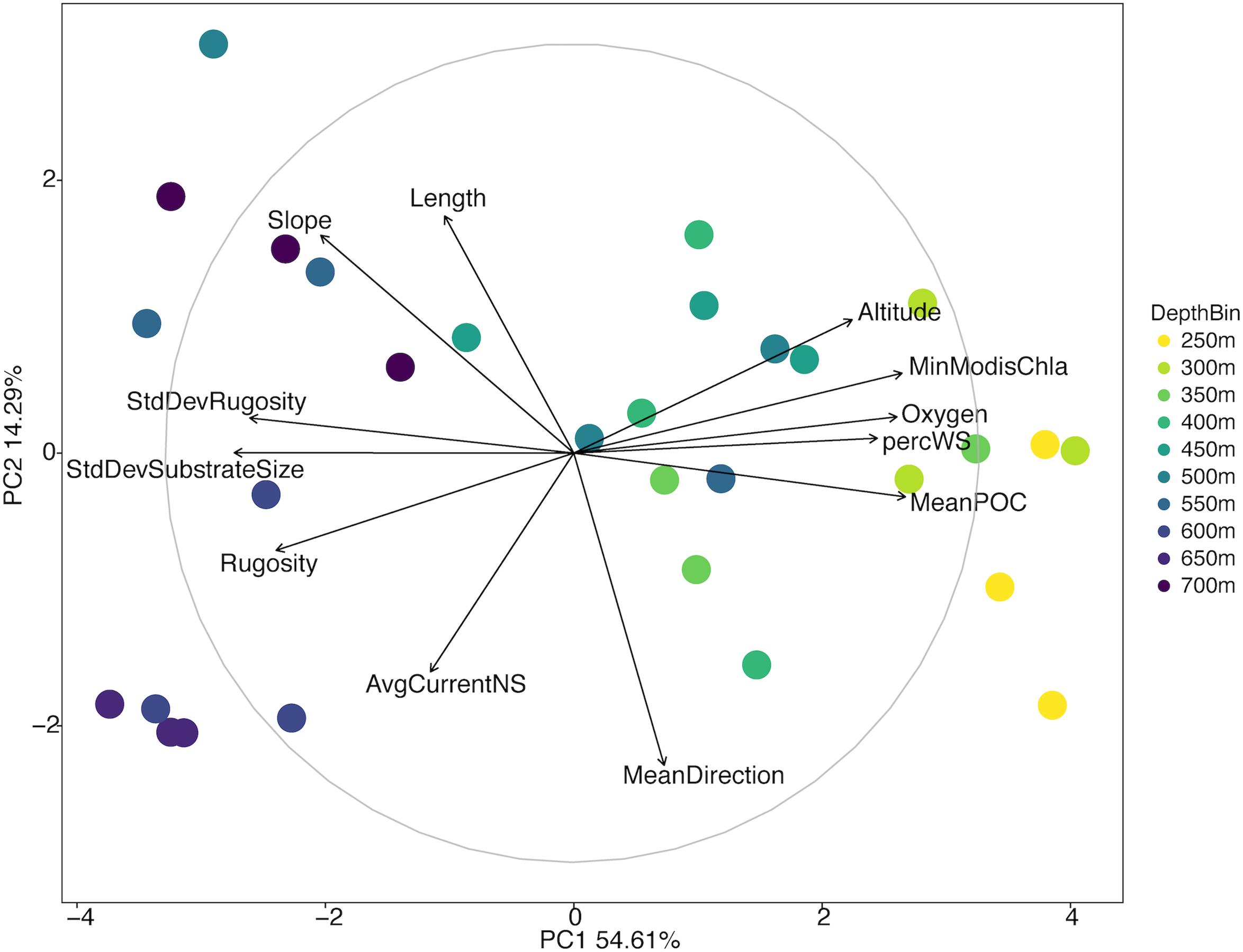
Figure 2. Principal components analysis diagram of environmental variables of the North side of Mokumanamana. Each point represents a single 1 km transect coded by depth.
Overall the North side showed an increase in abundance of Alcyonacea, Antipatharia, Actiniaria, holothurians, urchins, and ophiuroids with increasing depth (Supplementary Figure S1). Sea pens, arthropods, and asteroid sea stars were most abundant at shallow depths (250 and 300 m) while sponges and corallimorpharians were highly abundant at 450 and 500 m. Univariate diversity metrics show a general trend of increasing species richness (Figure 3A) and Shannon-Weaver index (Figure 3B) with increasing depth, though depth bins at 450 and 500 m do not follow the trends as they have much lower Shannon-Weaver indices, likely due to a low evenness component (Figure 3D). Simpson’s Dominance (Figure 3C) was generally low except for the 450 and 500 m transects due to the highly abundant corallimorpharians. Evenness is generally high over the North side except at 250 m and again at 450 and 500 m (Figure 3D). The 450 m depth bin was the most variable for all three indices.
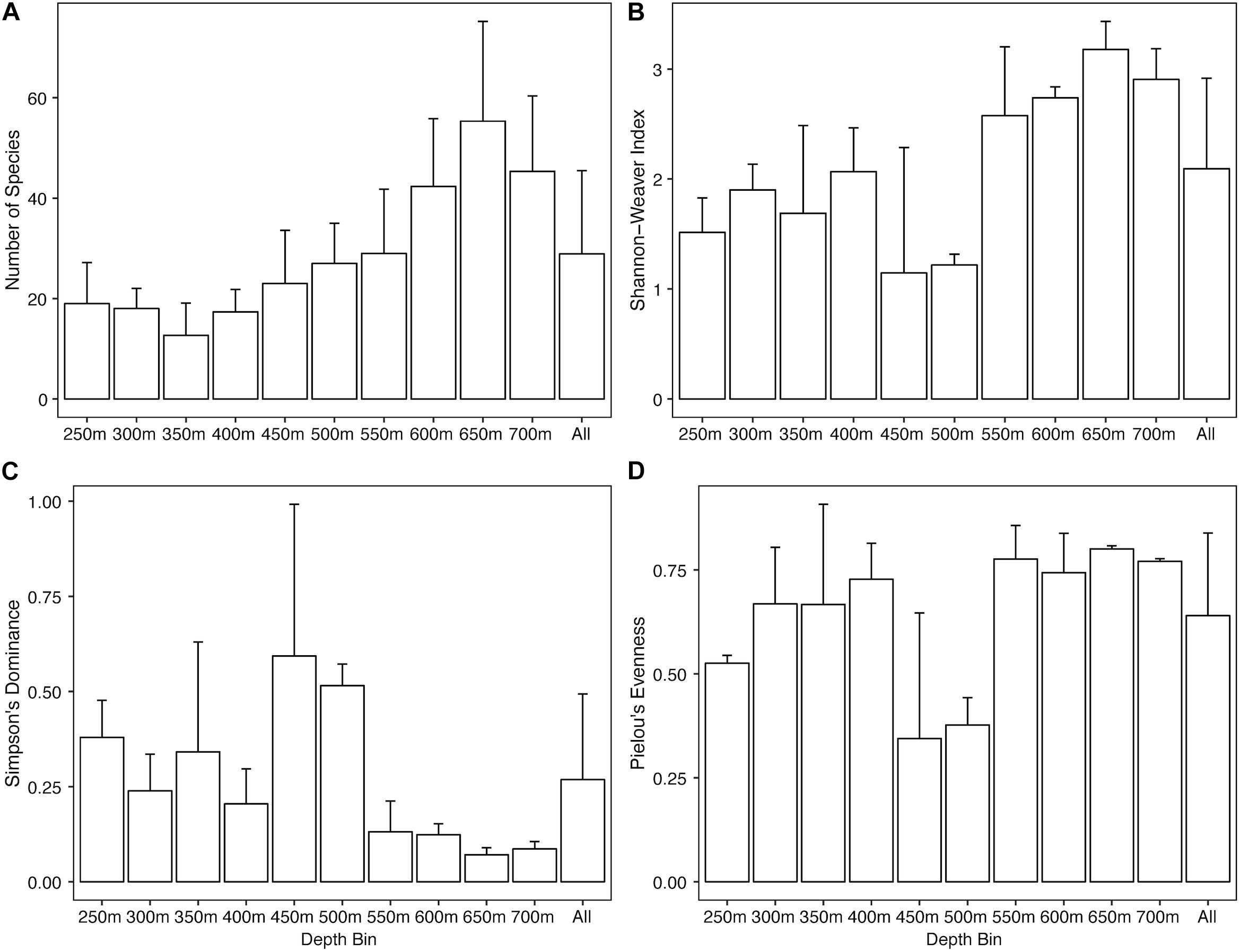
Figure 3. Bar plots of univariate diversity metrics for the North side of Mokumanamana by depth. Panels: (A) species richness, (B) Shannon-Weaver’s Index, (C) Simpson’s Dominance Index, (D) Pielou’s Evenness Index.
ANOSIM analysis for assemblage structure overall showed a significant difference globally for unordered depth bins (R = 0.78, p = 0.001), but pairwise comparisons between depth bins showed no significant difference between any two pairs (Supplementary Table S3). The hierarchical cluster of faunal assemblage data (Figure 4) shows three groups defined by depth relationships with shallow (250–350), mid-depth (400–500), and deep (550–700) transects clustering at 85% dissimilarity. The 400 m transects do not neatly fit into this pattern, and instead one replicate falls into each of the three clusters, but otherwise the assemblage grouping shows a strong depth relationship. When the environmental data are correlated to the assemblage structure for the North side of Mokumanamana three factors describe most of the variability: rugosity, oxygen, and mean POC (Figure 5). These three factors were highlighted by both the “bioenv” routine in the R vegan package and by the DISTLM routine in PRIMER-E (Table 1), however, the AIC value for the best model with three parameters was only 0.26 better than the model with only oxygen and mean POC. Oxygen has the strongest correlation with dbRDA1 (0.97), and this axis explains 48.38% of the variation in the model. dbRDA axis 2 explains 39.70% of the variation and is most strongly correlated to mean POC (0.63). Rugosity does add a small proportion of explained variance compared to a dbRDA model of just oxygen and mean POC, and is the most independent of the three variables (VIF = 1.65) (Table 1). In general, shallow transects had higher POC and oxygen concentrations and lower rugosity than deep transects.
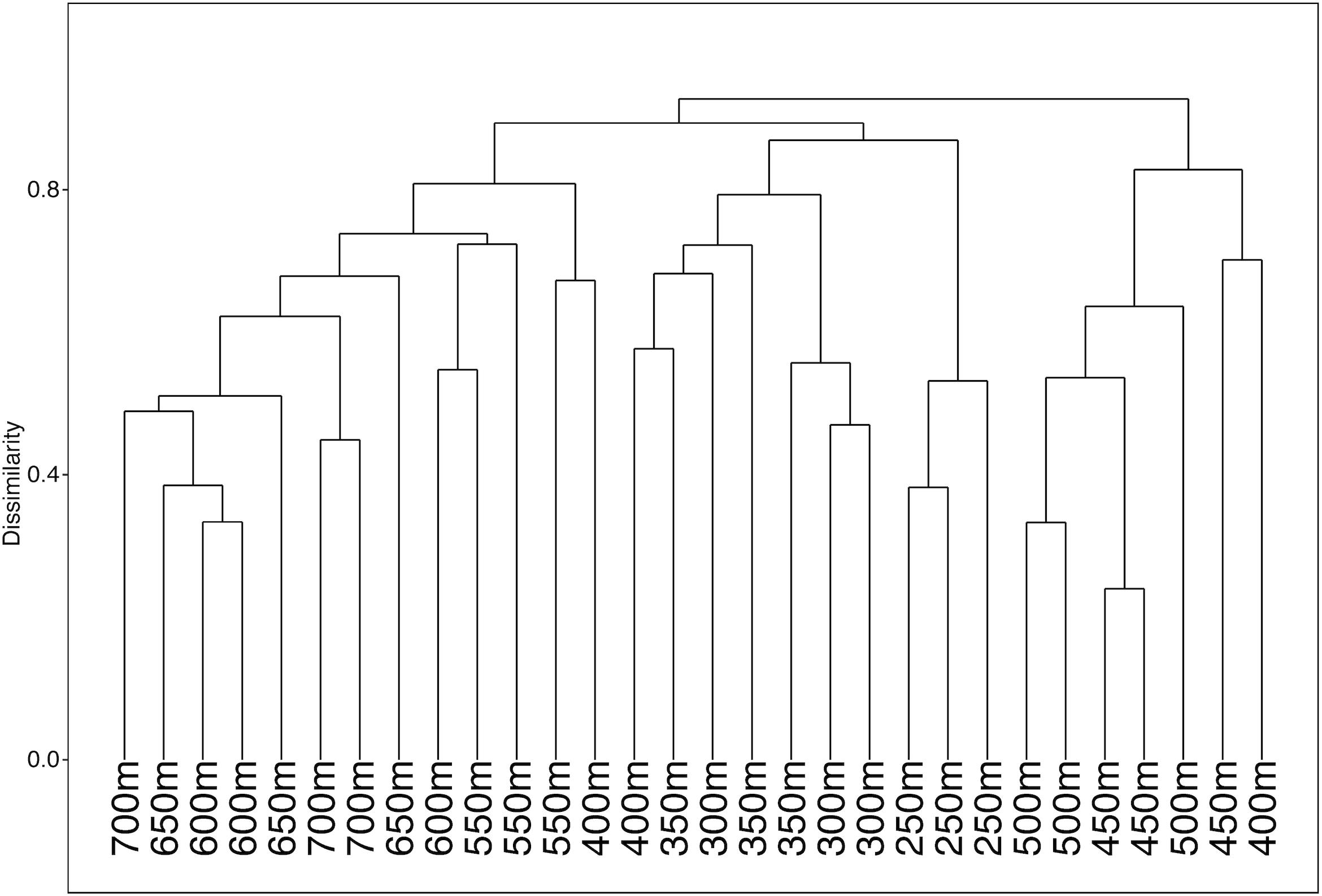
Figure 4. Hierarchical cluster diagram for the North side of Mokumanamana for transects labeled by depth bin.
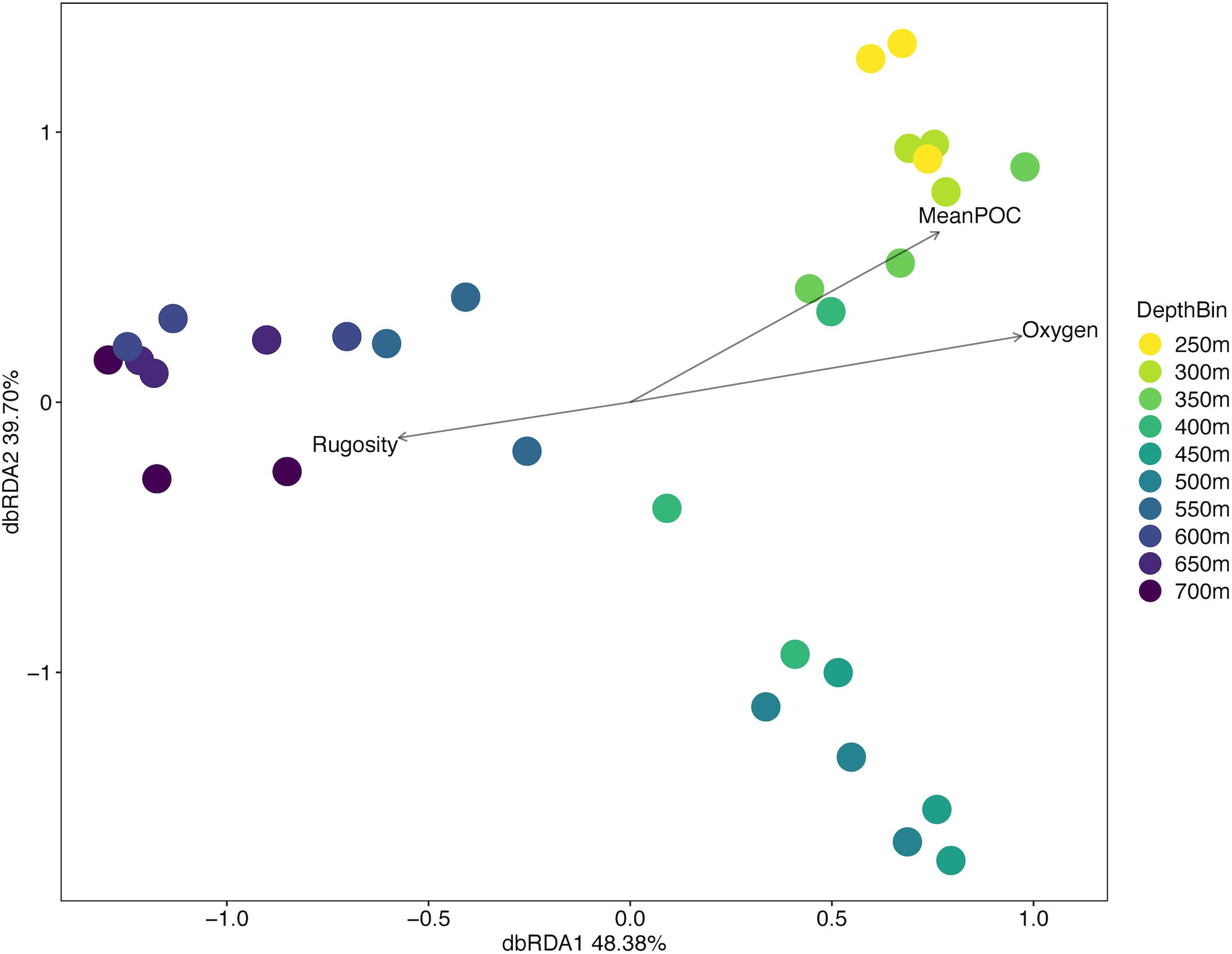
Figure 5. Distance-based redundancy analysis diagram for the North side of Mokumanamana coded by depth.
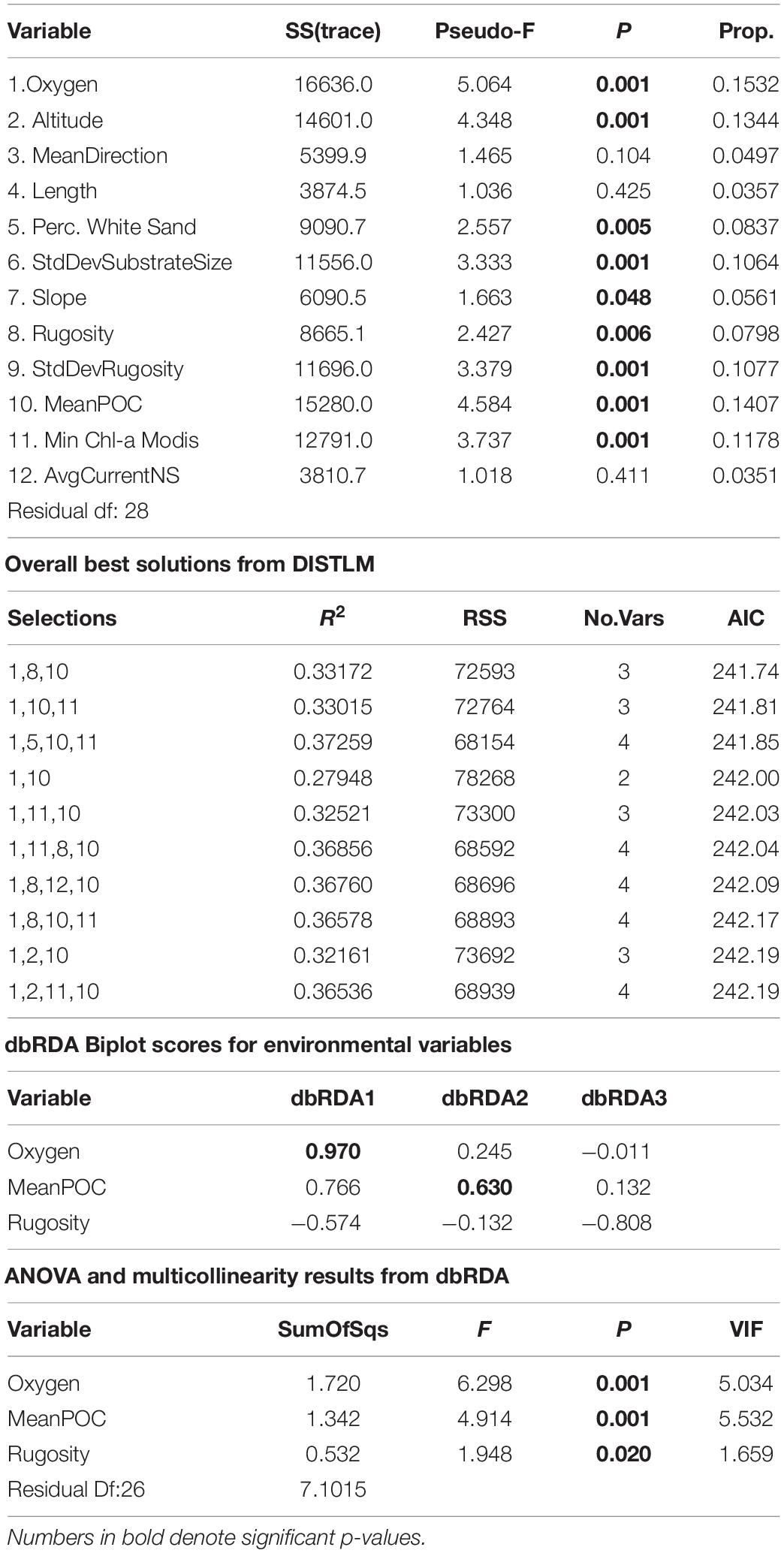
Table 1. DISTLM and dbRDA scores for the North side of Mokumanamana.
Mokumanamana Overall
Once the scales of the general trend of species turnover with depth were found from the North side, the two remaining sides were analyzed at 100 m depth intervals to allow for more efficient analyses. There was a broad range of variation in the environmental data collected from Mokumanamana as a whole (Supplementary Table S1); oxygen and temperature decreased with depth and were very similar for all three sides with ranges of 46–242 μM and 5–16°C, respectively. Mean POC decreased with depth on the North and West sides with ranges of 33–39 mg/m3 and 36–48 mg/m3, but was more consistent on the South side around 31 mg/m3. Percent sediment also generally decreased with depth, but the North side overall had more sand (35–98%) than the West (22–99%) or South (4–89%) sides. Rugosity increased with depth, and was more consistent across all sides of Mokumanamana. Mean direction was differed between the West (range 0.22–1.32) and South sides (range −1.36–0.12) while the North side encompassed the full range of values (−1.49–1.53); however, mean direction showed no trend with depth at any side. Average surface currents were consistent across depths and instead varied by side with the average north-south surface current faster on the West side (range 0.06 to 0.09 m/s, overall northward direction) and the surface east-west current faster on the North side of the seamount (range −0.11 to −0.13 m/s, overall westward direction).
Of the initial 31 environmental parameters, 19 were removed due to correlating or missing data (Supplementary Figure S2). The PCA for all three sides of Mokumanamana shows gradients in the environment by both depth bin and by the side of the seamount (Figure 6 and Supplementary Table S4), with the South side trending toward the bottom of the ordination and shallower depths to the left. PC1 describes 38.8% of the environmental variability and is most strongly correlated with oxygen, rugosity, the standard deviation of rugosity, and percent sediment. Transects generally cluster along PC1 by depth from left to right. Similar to the North side PCA (Figure 2), shallower samples had higher oxygen concentrations, lower rugosity, and more consistent substrate coverage of white sand while deeper samples had more pebbled substrate and rocky outcrops. PC2 describes 14.72% of the variability and is most strongly correlated with mean direction and the average east-west surface current. Along PC2 samples generally cluster by the side of Mokumanamana with the southern transects especially differentiated from the North and West transects due to a much weaker westward current and rocky outcrops at deeper transects that at times reached 25 m high.
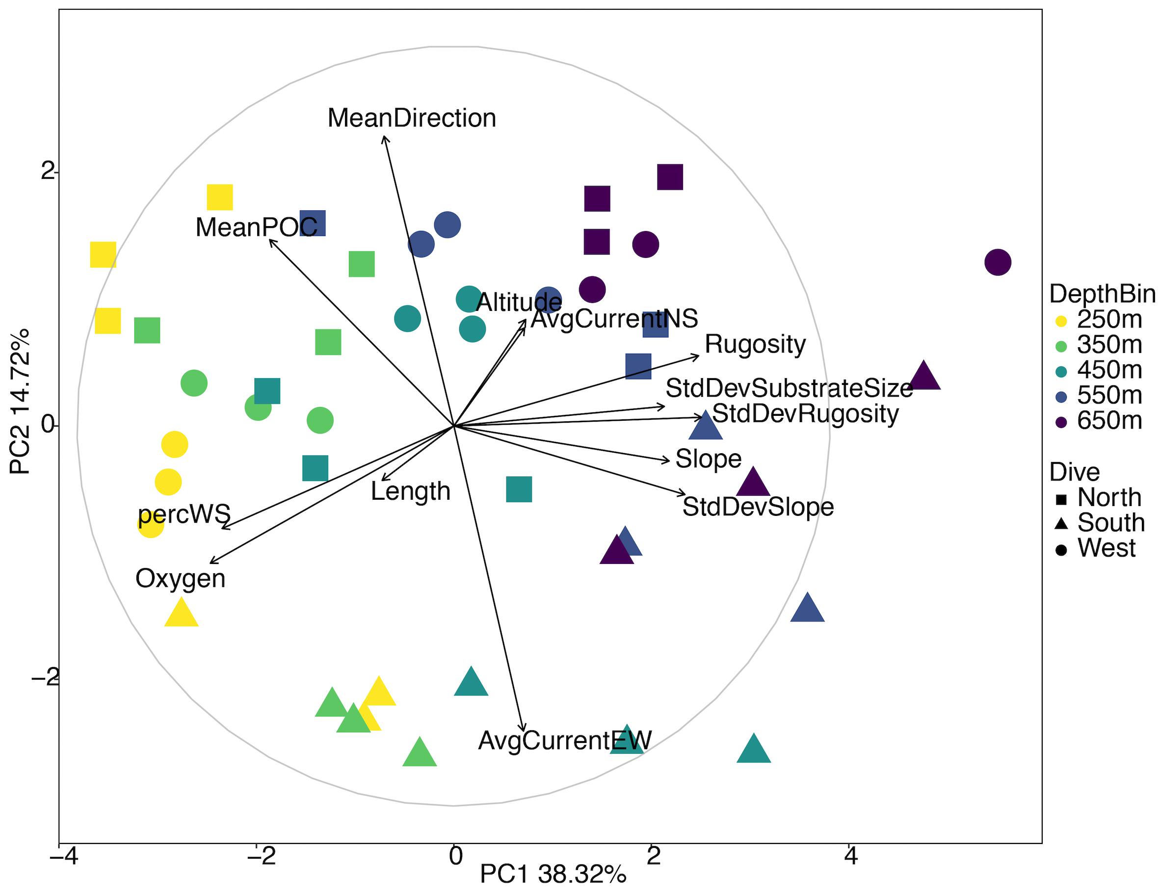
Figure 6. Principal components analysis diagram of environmental variables for three slopes of Mokumanamana. Each point represents a single 1 km transect coded by depth and side.
The abundances of benthic invertebrates were different among the sides of the seamounts (Supplementary Table S5), overall the West side had nearly three times as many animals compared to the North and South sides overall, with the largest differences in arthropods, cnidarians, and echinoderms (Figure 7). Arthropods on the West side were mainly comprised of squat lobsters, cnidarians mainly of cup corals, corallimorpharians, and the sea pen Anthoptilum grandiflorum. The West side was also characterized by high numbers of benthic ctenophores of the Lyrocteis genus. Cnidarians of the North side were mostly comprised of sea pens Kophobelemnon stelliferum and Virgularia abies, and the South side mainly Metallogorgia melanotrichos and Anthomastus sp. Sponges were more abundant on the North and South sides than the West side, and on the North side sponges were dominated by Sericolophus sp. while the South side was dominated by Farrea sp. Univariate diversity metrics did not vary by side, but did by depth and the interaction of depth and side (Supplementary Table S5). Overall the three slopes showed an increase in species richness (Figure 8A) with increasing depth, and the West and North sides show an increase in Shannon-Weaver and Pielou’s evenness with depth and a decrease in Simpson’s Dominance, though the 450 m depth bin for the North side as noted, still does not fit the overall trend (Figures 8B–D). While the West side has the highest abundance, the South side generally had a higher diversity as measured by the Shannon-Weaver index and higher evenness as measured by Pielou’s Evenness for 250, 350, and 450 m depth bins. The North side has the highest diversity for 550 and 650 m depth bins (Figures 8B,D). Diversity metrics are the most consistent across depth bins for the South side.
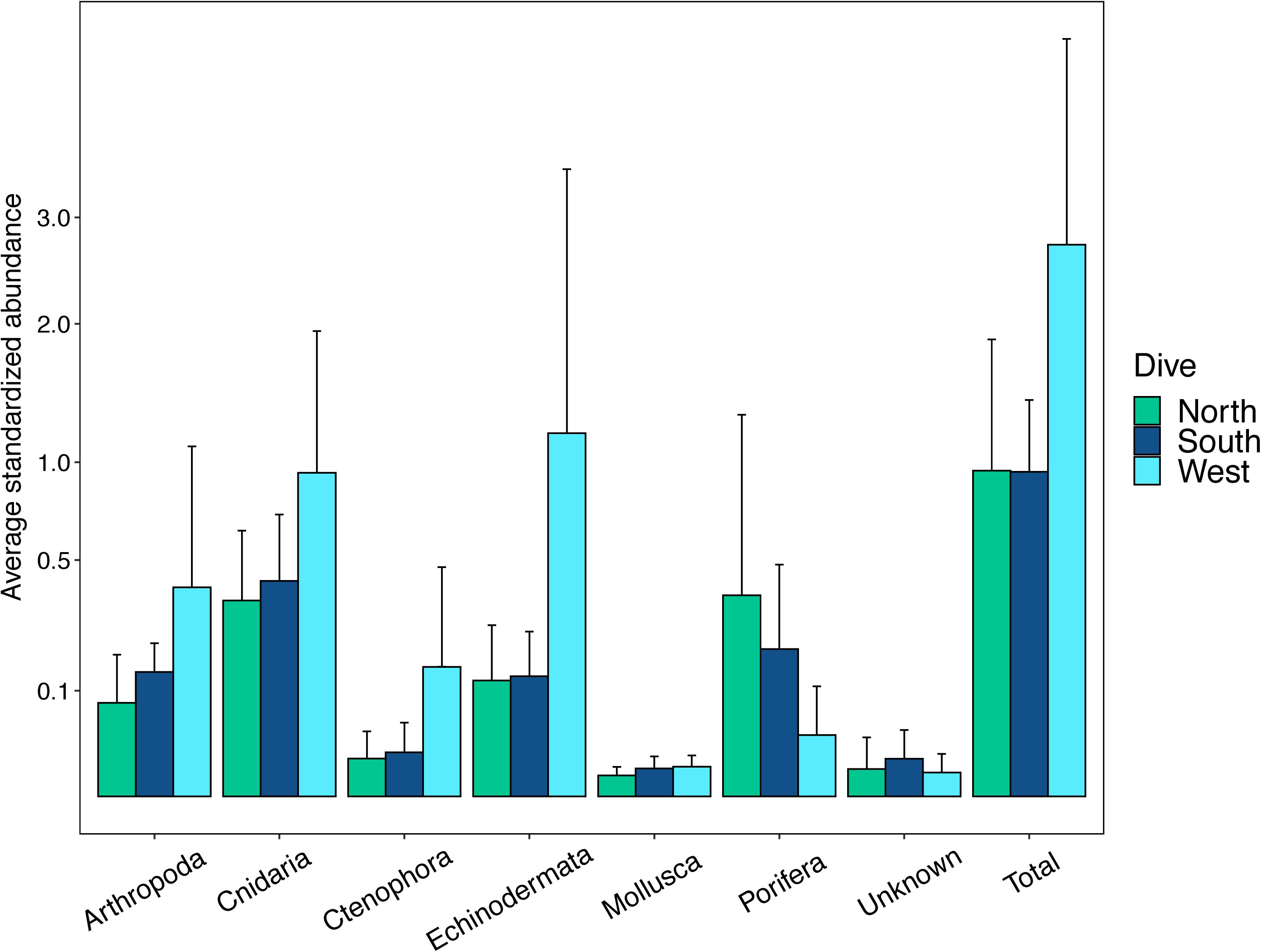
Figure 7. Abundances of major phyla on the three slopes. Abundances are standardized as the number of individuals per number of photos taken in each transect. The y-axis values are square root scaled for easier visualization of values.
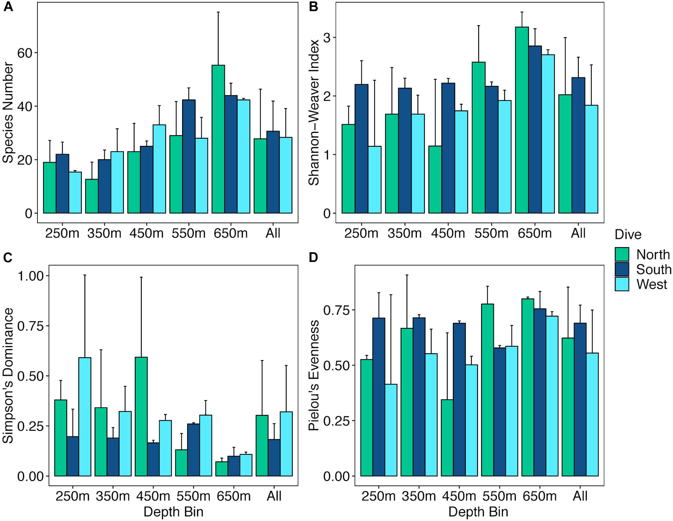
Figure 8. Bar plots of diversity metrics for three slopes of Mokumanamana by depth. Panels: (A) species richness, (B) Shannon-Weaver’s Index, (C) Simpson’s Dominance Index, (D) Pielou’s Evenness Index.
Crossed ANOSIM of assemblage structure overall by depth bin and side showed significant differences both between depth bins (global R = 0.80, p = 0.001) and sides of the seamount (global R = 0.807, p = 0.001). Pairwise comparisons showed significant differences between all pairs of depth bins and between all comparisons of the sides of the seamount (Supplementary Table S6). Beta diversity was also high (Supplementary Figure S3), and values range from 0.90–0.95 (max. value of 1.00). Beta diversity on all three slopes of Mokumanamana was mostly defined by the substitution of species along the depth gradient rather than the nestedness of species, meaning that the species turnover was not defined as a loss of species richness but rather a replacement of species with changes in depth. Within a depth bin, beta diversity was also high between the three sides of Mokumanamana (0.81–0.88), and 24.8% of all morphospecies were found on only one side of the seamount, 24.9% were found on only two sides, and 50.3% of all morphospecies were found on all three sides.
Multivariate analyses also show that both depth and side have strong influences on the faunal assemblage structure of invertebrates on Mokumanamana. Hierarchical cluster analysis first shows two samples from the North side at 450 m are outliers from the rest of the assemblage data (Supplementary Figure S4). This is likely due to dense patches of Sericolophus sp., and the two outlier transects are subsequently removed from the rest of the analyses. The clustering structure of the remaining samples does not change once the outliers are removed and a trend of samples from the same depth bin and slope being more similar can be seen (Figure 9), though three transects do instead cluster with other depths (a South 250 m) and other slopes (a West 250 m and a North 550 m). The K-means clustering algorithm defined nine clusters by Bayesian modeling that can be seen in the NMDS plot and map in Figure 10. Eight of the clusters each contain 1–2 depth groups and 1–2 sides of the seamount. Only cluster 5, which was comprised of 450 m depth transects, had at least 1 transect from each of the 3 sides. Notably, the South 550 m transects form group 7, North 550 and 650 m transects form group 8, and West and South 650 m transects form group 9. The only deviation from shallow, mid-depth, and deep groupings that originally came out in the North-side-only analyses within the k-means groups is in group 6 where a 350 m transect clusters with its fellow West-side 550 m transects.
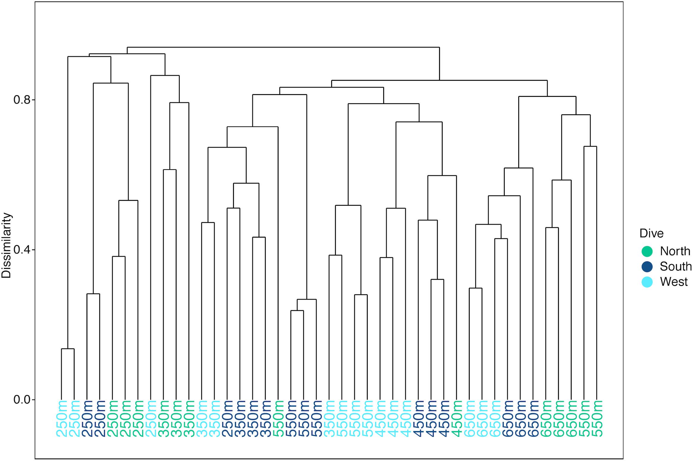
Figure 9. Hierarchical cluster diagram for three slopes of Mokumanamana for transects labeled by depth bin and color coded by side.
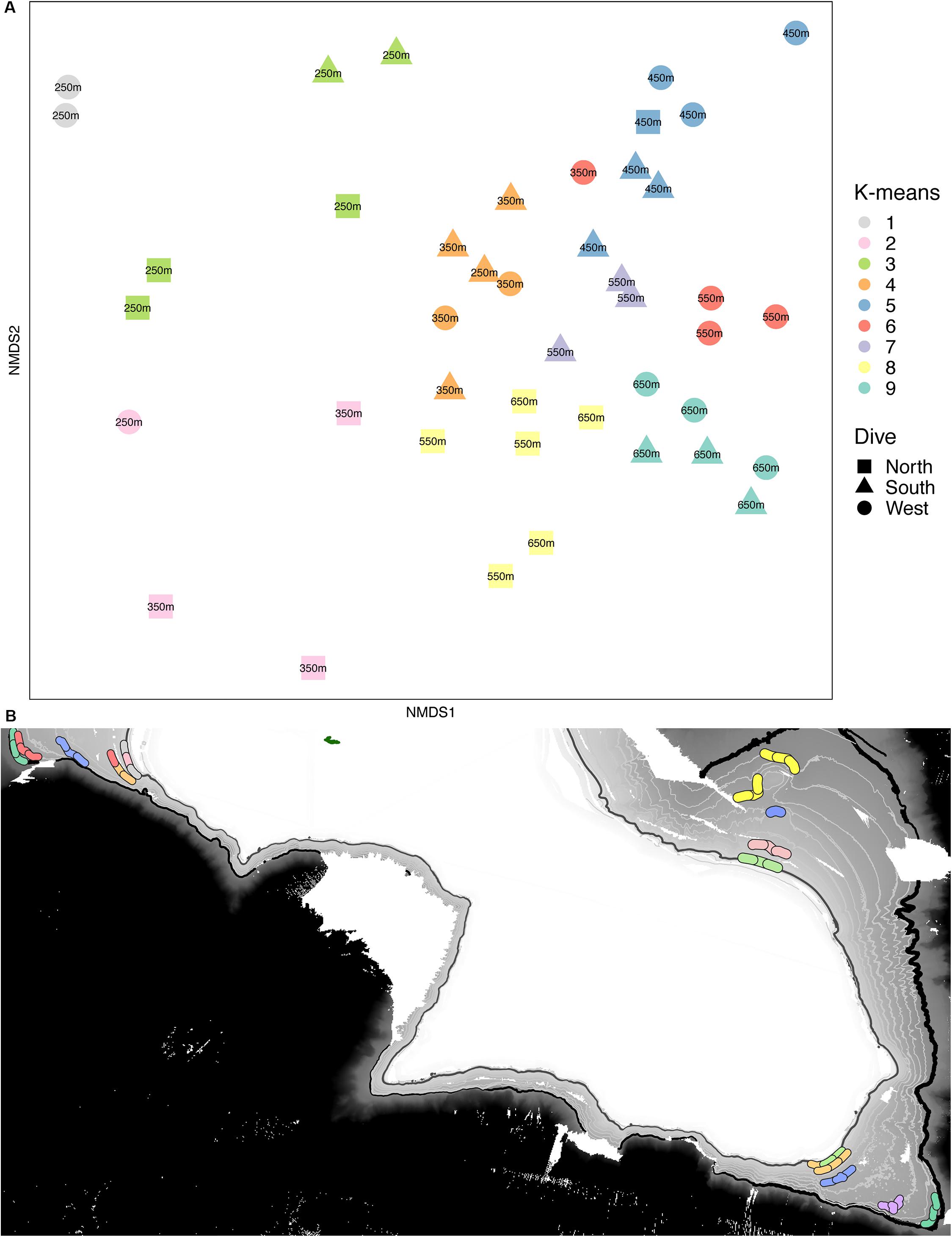
Figure 10. (A) Non-metric multidimensional scaling plot for assemblage structure of Mokumanamana color-coded by k-means clusters labeled by depth bin. (B) map with locations of transects denoted by their k-means clusters color code from (A).
When the assemblage structure is modeled with the environmental data there was still a strong effect by depth and side. Of the top 10 DISTLM models, the best one included 10 variables (Table 2); however, no model AIC was significantly higher than any other so all eleven variables indicated by DISTLM were analyzed together. VIF shows mean direction is the most independent variable in the model (v = 1.95) while oxygen is the least independent (v = 6.59). Standard deviation of slope was removed due to a VIF > 10. Ten environmental variables were included in the final model, and eight are significantly correlated to the assemblage data (p-value range: 0.004–0.001); the non-significant variables are transect-length and slope (Table 2). In Figure 11, dbRDA1 was most strongly correlated to oxygen and percent sediment and described 27.69% of the constrained (modeled) variation, while dbRDA2 was most strongly correlated to mean POC and average eastward current and explained 18.68% of the variation in the model. Ten axes were needed overall to explain all variation in the model, but only the first four axes were significant (p ≤ 0.0002).
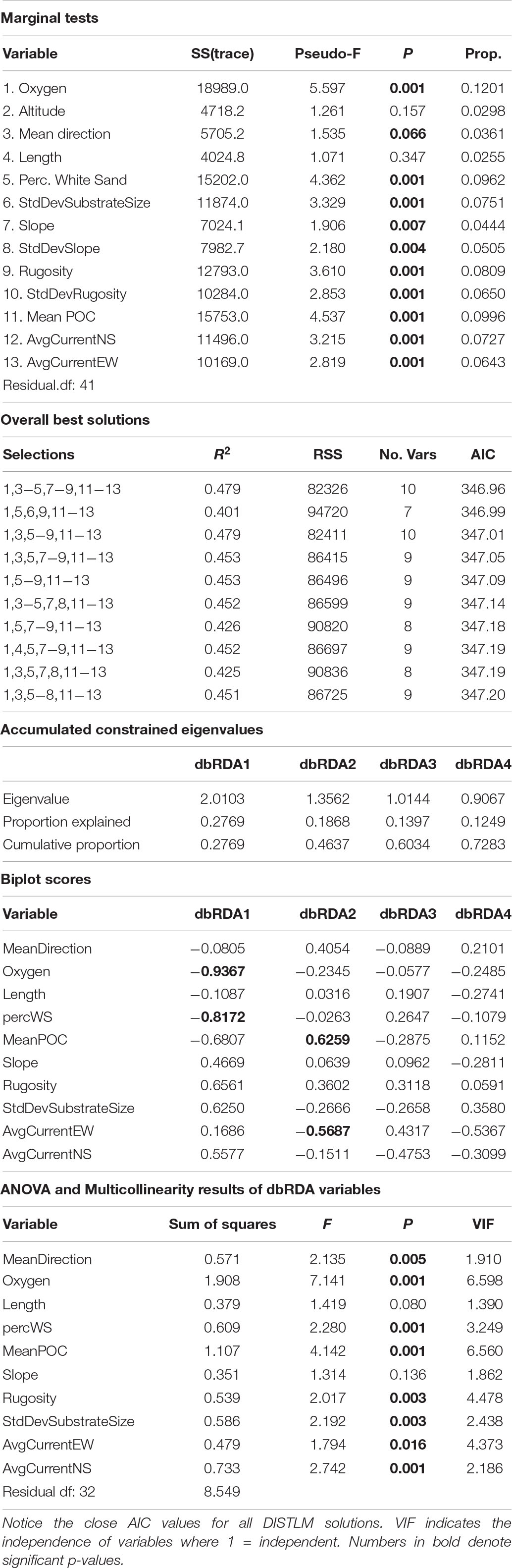
Table 2. Results from DISTLM model and dbRDA analysis for Mokumanamana overall.
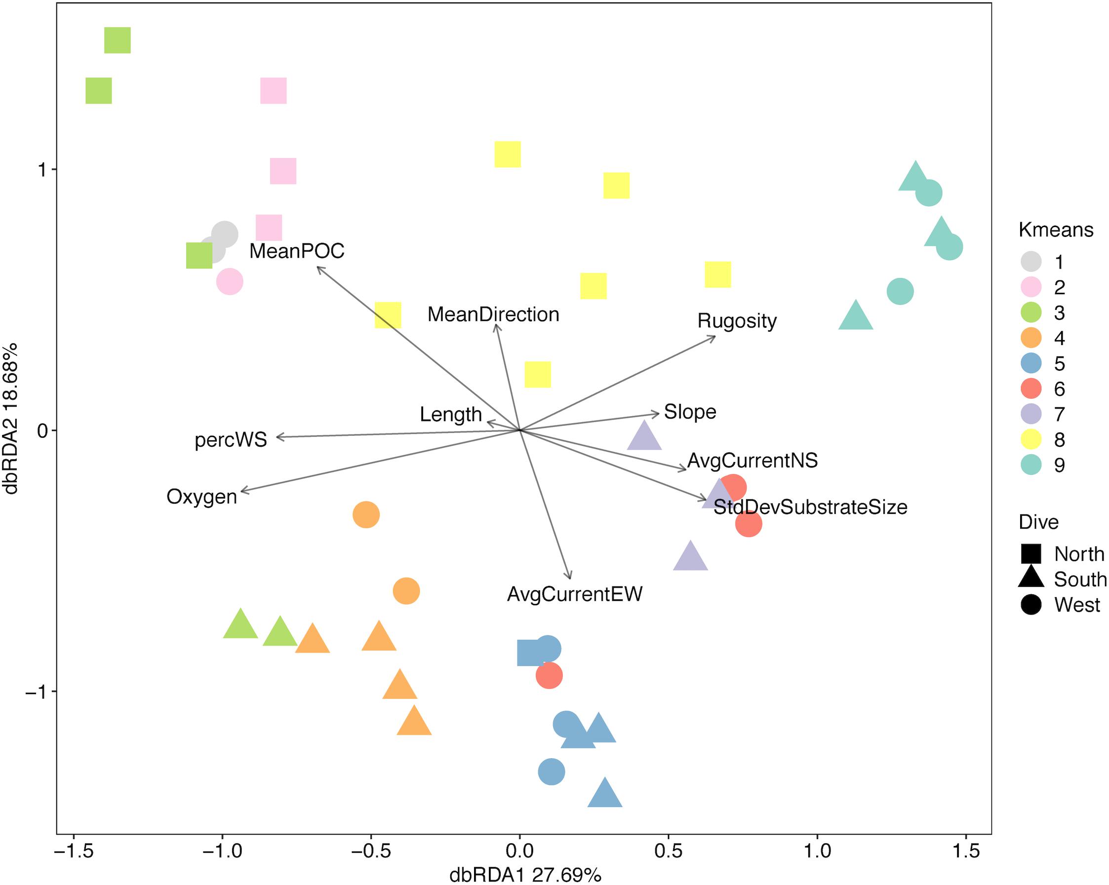
Figure 11. Distance-based redundancy analysis diagram for three slopes of Mokumanamana.
When the environmental values were overlaid on the assemblage structure NMDS, the variables that were correlated with the differences between depth bins and sides become more apparent. One-way ANOVAs were run for each variable by depth and side to compare whether the variable changed more vertically or horizontally (Supplementary Table S7). Figures 12A–D, shows those variables found significant in the dbRDA that changed most with depth. Shallower samples have a higher percent sediment (Figure 12A), which also decreases the rugosity (Figure 12C) and variability in the slope (Figure 12D) in these areas. Deeper samples may have up to 50% soft sediment, but the high rugosity and variability in the slopes of these transects is due to more exposed hard substrate. Oxygen decreased quickly with depth (Figure 12B). Figures 12E–H, shows those variables that changed most with the side of the seamount. Mean surface POC (Figure 12E) was highest on the North side and lowest on the South side. Mean direction (Figure 12F) was more consistent on the West side while transects on the South side were the most variable. The 8-year average surface currents do not change direction over Mokumanamana, with the predominantly northward current weakest on the North side (Figure 12G) and strongest on the West side. The east-west component of surface current was predominantly westward flowing and was strongest on the northern slope, but weakest on the South facing slope (Figure 12H; more negative values are stronger westward currents).
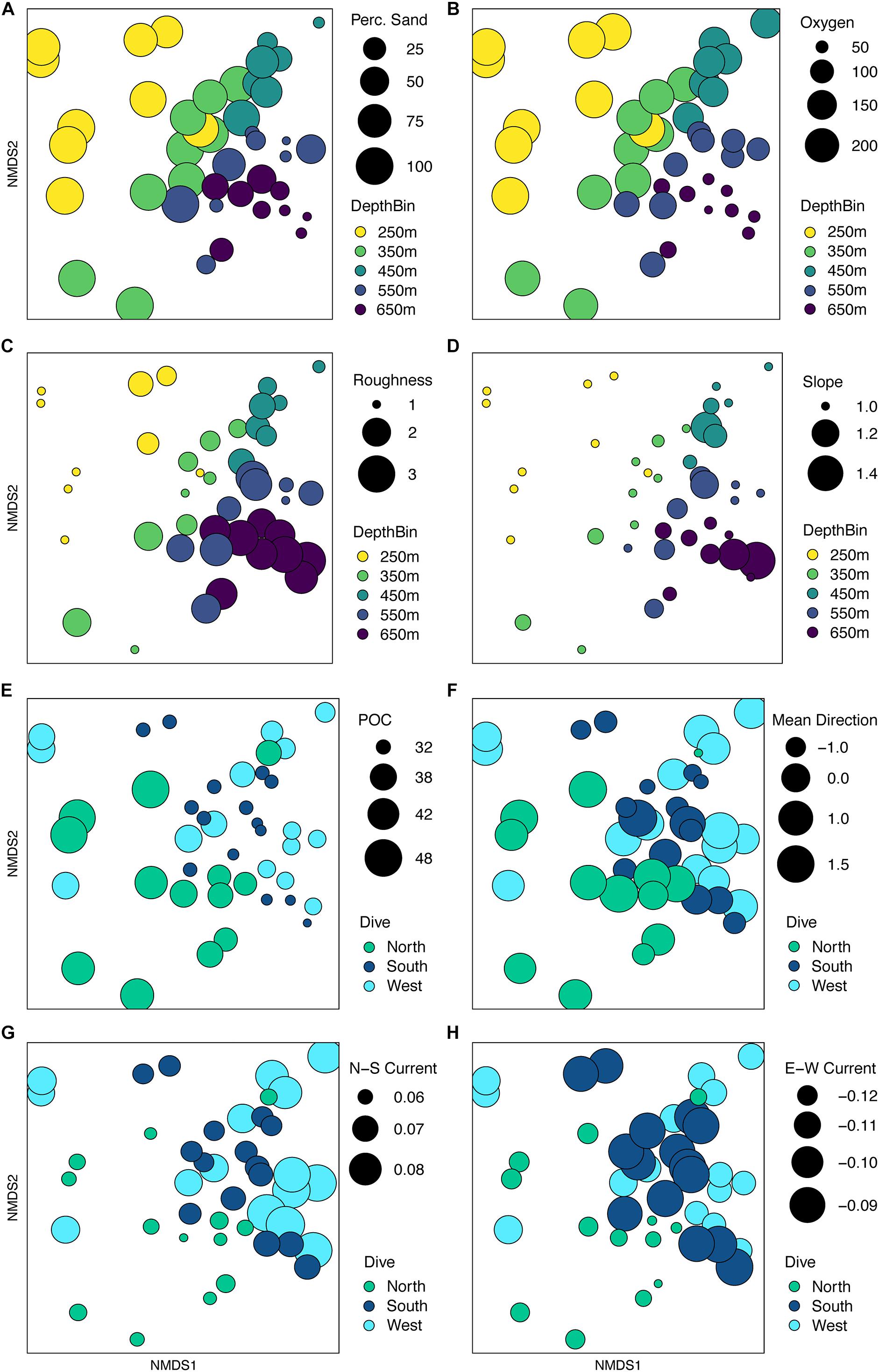
Figure 12. Non-metric multidimensional scaling plot for assemblage structure of Mokumanamana from Figure 10 with overlay of environmental gradients. Circle size is relative to values of variables that change with depth or dive. Panels: (A) percent sediment, (B) oxygen (μM), (C) roughness, (D) standard deviation of slope, (E) mean particulate organic matter (mg/m3), (F) mean direction, (G) northward current (m/s), (H) westward current (m/s).
The number of species that best define each k-means group from SIMPER analysis is generally small, especially for shallower groups (Supplementary Table S8). Figure 13 uses the abundance data of the species designated by SIMPER and shows the square root transformed relative abundances of those throughout the dataset. Groups 1–3 are shallow transects at 250 m, and they are generally comprised of few species. Group 1 was strongly defined by the numerous squat lobsters though V. abies sea pens were also common. Group 2 was defined by the sea pen K. stelliferum and an asteroid Calliderma sp. along with squat lobsters. Cup corals were present, but not highlighted as significant by SIMPER. Group 3 was defined by the highly abundant V. abies as well as Brisingid sp.3 and the cidaroid urchin Stylocidaris calacantha. Groups 4–6 were more mid-depth transects (350–450 m) though one 250 m transect and three 550 m transects from the West side fell into this group. All three groups were defined by an abundance of shrimp. Group 4 was also defined by the presence of spatangoid heart urchins and K. stelliferum. Group 5 was comprised of all the transects from 450 m and was defined by cup corals Caryophyllid sp., benthic ctenophores Lyrocteis sp., and corallimorpharian Corallimorphus pilatus. Group 6 was defined by shrimp and C. pilatus. Groups 7–9 were comprised of 550 and 650 m transects, and Group 7 was defined only by shrimp and Farrea sp. sponges. Groups 8 and 9 showed a greater number of species contributing to the within group similarity, consistent with the higher diversity found on the deeper transects and were defined by numerous species of corals and echinoderms, including the corals Anthomuricea tenuspina, Metallogorgia melanotrichos, Chrysogorgia stellata, and holothurians Hansenothuria benti and Orphnurgus sp.
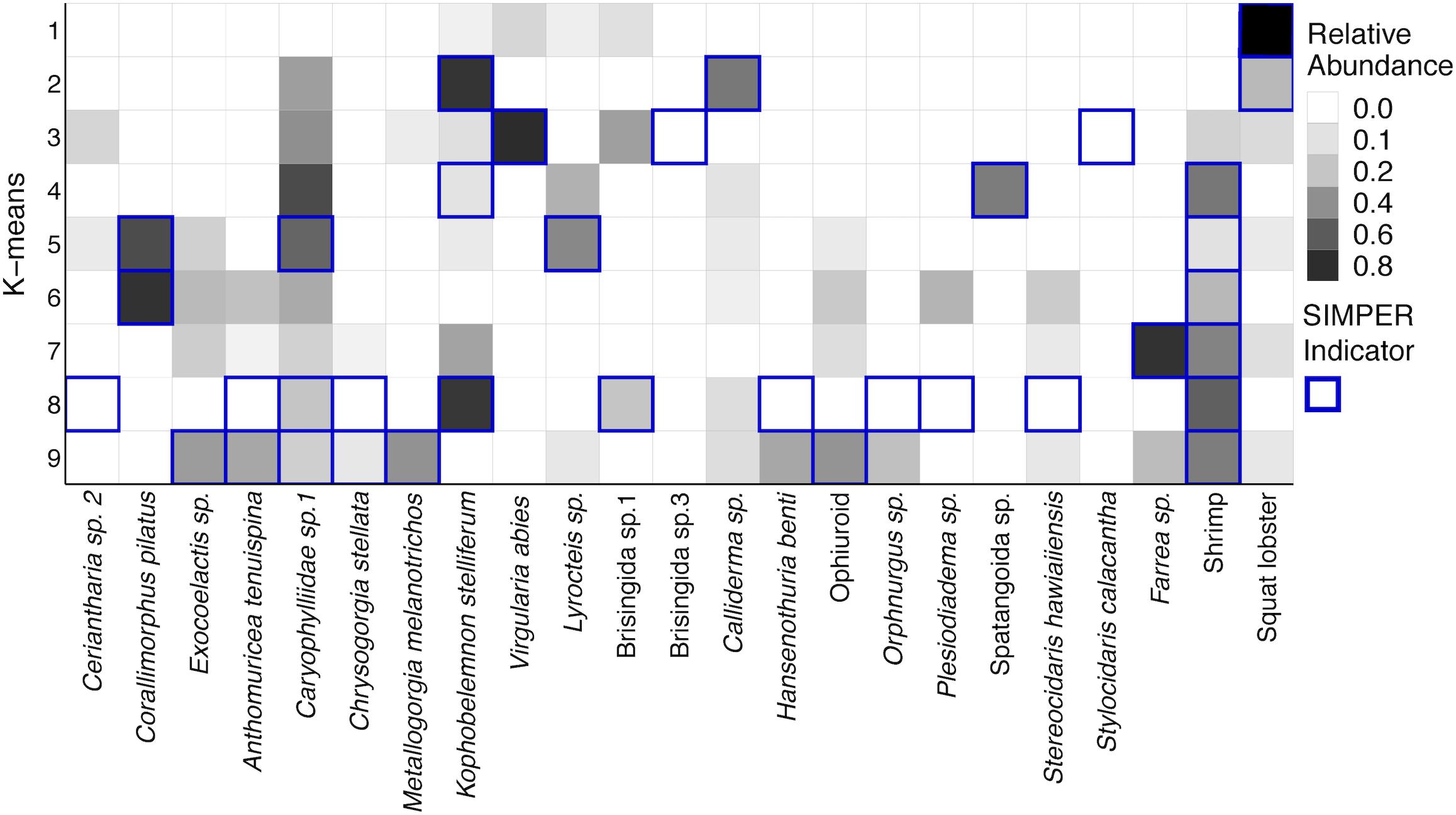
Figure 13. Heatmap of the square root transformed relative abundances of species that define k-means clusters from SIMPER analysis. Along the row for each k-means group, the species indicated by SIMPER analysis as drivers of within-group similarity are outlined in dark blue.
Discussion
Environmental Gradients at Fine Scales
Opportunities for intensive investigations of variability in faunal communities and environmental parameters on the scale of a single seamount feature have been rare, but have suggested that there may be significant habitat heterogeneity on individual seamounts, which can be expected to translate into significant variation in community structure and species composition within a single feature (Baco, 2007; McClain et al., 2010; Bo et al., 2011; Long and Baco, 2014; Thresher et al., 2014; Morgan et al., 2015; Victorero et al., 2018a; Mejia-Mercado et al., 2019). The data presented here represent one of the most extensive investigations of a single seamount, with over 150 km of the untrawled seamount Mokumanamana surveyed using an AUV. Despite the relatively narrow depth range surveyed (200–700 m), enough variability was observed in habitat parameters among transects that depth and the different sides of Mokumanamana were apparent in the ordination plots of environmental data, confirming the presence of high habitat heterogeneity on this seamount. In particular, substrate size, mean POC, oxygen, percent sediment, rugosity, chlorophyll-α values and mean direction were strongly correlated with variation among transects in the PCA on the North side (Figure 2); while in the PCA for all three sides, oxygen, rugosity, percent sediment, mean direction and the average east-west surface current were the significant factors (Figure 6).
Even though depth was not included in the data used for the PCA, there was a clear depth gradient along the PC1 axis, correlated to several substrate parameters. The slope became steeper with increasing depth, percent sand decreased, and roughness increased (Figure 12). Larger outcrops and boulders became the dominant substrate forms at deeper depths, though patches of high sediment cover were still present. Though some deep transects had sediment as the dominant substrate type, there were still secondary substrate types (Mortensen and Buhl-Mortensen, 2004; Neves et al., 2014) of boulders, cobble, or hardpan, which can provide hard substrate habitat. All of this contributed to a general increase in substrate complexity (variability in substrate size and type, rugosity, and slope) with depth, which increases the types of habitats available, likely contributing to the higher diversity observed on deeper transects (Figures 3, 8).
In contrast to these substrate parameters, oxygen decreased with depth (Figure 12B). Decreases in oxygen would usually suggest decreased species richness and diversity (e.g., Wishner et al., 1990; Gooday et al., 2009), instead of the increases seen on Mokumanamana (Figures 3, 8), but while oxygen levels do decrease with depth from around 250 μM at 250 m to 50 μM at 650 m (8 mg/L to 1.6 mg/L), they do not approach lethal or sublethal values for the dominant benthic invertebrates on this feature (Vaquer-Sunyer and Duarte, 2008), with one exception being crustaceans. Vaquer-Sunyer and Duarte (2008) found crustaceans to be affected by oxygen levels less than 63 uM (2 mg/L) and to have the highest sensitivity to low oxygen values. Crustaceans overall are still present at deeper transects, but in much lower abundances than at 250 m, which could suggest more sensitive species are restricted to shallower depths. However, increased rugosity at deeper transects could also make counting smaller crustaceans from imagery more difficult. Shrimp and palinurid lobsters are the only crustaceans to increase with depth, suggesting these organisms are less sensitive to low oxygen concentrations.
Oxygen was strongly correlated with temperature and conductivity, which predicated the removal of these two parameters prior to multivariate analyses; however, these variables could still have an influence on assemblage structure. The observed temperature range on Mokumanamana (5–16°C) is very similar to other features studied in the NWHI in the same depth range (Parrish, 2007). Temperature is known to influence physiology and metabolism, which in turn can influence biodiversity and assemblage structure in an ecosystem. Diversity in the deep-sea has a unimodal relationship with temperature, with the peak expected around 6°C (Yasuhara and Danovaro, 2016). Diversity on Mokumanamana follows the expected trend with the highest values of species richness and diversity occurring around 5°C. Conductivity ranged from 3.2 to 4.2 S/m and is also within the expected range for this area (Tyler et al., 2017). Conductivity/salinity is not expected to be influential in many deep-sea assemblages as it is considered mostly constant (Roberts et al., 2009).
The three sides of Mokumanamana were also apparent in the environmental PCA plot with the South side being more distinct from the North and West than either of those were from each other (Figure 6). Even though the North and West sides were more similar to each other based on the available environmental data, this did not translate into comparable diversity and abundance metrics. The West side had much higher abundances especially among the echinoderms, arthropods and cnidarians, while the North had the highest abundance of sponges. The West side was the least diverse and the South side had the lowest evenness of the three sides (Figures 7, 8).
Factors that varied most strongly among the sides were surface POC, mean direction, and direction of the surface currents (Figure 12). POC was highest on the North side and lowest on the South. Higher POC values would typically be related to increased abundance and biomass (e.g., De Rijk et al., 2000), yet the highest abundances of animals, except sponges, occurred on the West side (Figure 7). The range of POC is relatively narrow (31–48 mg/m3), and the values are still oligotrophic for the feature as a whole. The data are also surface POC values, and the interaction of surface and deeper currents may affect the distribution of available POC by the time it reaches the slopes of the seamount. Seamount flanks have been shown to accelerate currents, generate internal tides, and trap mesoscale eddies along their flanks, especially on the west side of the seamount in the Northern Hemisphere (Genin et al., 1986, 1989; Eriksen, 1991, reviewed in White and Mohn, 2004). With the horizontal current component dominantly westward over Mokumanamana (Supplementary Figure S5), mesoscale eddies could be trapping sinking POC along the western flank, allowing for the nearly three-fold increase in abundance of invertebrates on that side. A parallel study of fishes on Mokumanamana found they were most abundant on the South and West sides, likely due to a higher prevalence of rocky substrate providing more protected areas for organic matter to accumulate (Mejia-Mercado et al., 2019). On seamounts in Tasmania, Thresher et al. (2011) found an extremely dense community, with much more biomass than was expected to be possible based on surface primary productivity above the features. Instead, they hypothesize that the biomass is supported by pulses of food advected from more productive waters further offshore. Other labile organic matter not measured from satellite data can also be more concentrated on seamount flanks; Kiriakoulakis et al. (2009) found increased concentrations of both suspended POC and polyunsaturated fatty-acids near the summit of Seine Seamount in the North Atlantic compared to open water at similar depths. Gori et al. (2014) found four species of cold-water corals were able to use free amino acids as a food source. Thus, in the oligotrophic waters above Mokumanamana, other organic compounds such as fatty acids, amino acids, and sugars could also be important food sources.
Species richness in the deep-sea generally increases with depth and peaks around 2000 m (Rex and Etter, 2010). The increase in species richness with depth on Mokumanamana (Figure 8A) follows this general trend. Overall, Mokumanamana had high alpha diversity and overall diversity, as described by Shannon-Weaver index, compared to other features within the NWHI at similar depths (Vetter et al., 2010), and were on average similar to the diversity of the Necker Ridge at depths of 1400–1800 m (Morgan et al., 2015). Surface primary productivity is similar on Necker Ridge to Mokumanamana, which may explain their similar levels of diversity despite the depth differences. Long and Baco (2014) surveyed comparable depths to the current study in a precious coral bed on the Island of Oahu in the Main Hawaiian Islands, but focused only on sponges and corals. That study had lower species richness, but higher abundances than Mokumanamana. Primary productivity is higher around Oahu and the Main Hawaiian Islands, which may explain the higher abundances found there (NOAA STAR Ocean Color, Wang and Jiang, 2018).
Assemblage Structure
On Mokumanamana, the environmental gradients that occur both vertically and horizontally have a strong effect on assemblage structure, augmented by biogenic structures of octocorals and sponges, which provide numerous landscapes for diverse assemblages to exist. Hierarchical clustering demonstrated a pattern of transects clustering mostly by depth, but also by side within depth clusters, resulting in 9 assemblage groups (Figure 9). The NMDS representation of assemblage structure shows that the 250–350 m depth transects have higher dissimilarity among them as compared to deeper transects (Figure 10). Within this depth range, all three sides had similar sandy habitats, instead current strength and mean POC vary among the sides and may be contributing to variation in assemblage structure. Within the faunal data, low evenness and low species richness at these depths (Figures 8A,D) may further contribute to their dissimilarity. The only k-means group with transects from all 3 sides, Group 5 at 450 m depth (Figure 10) stands out because many transects in this cluster have low evenness and the habitats were quite different between the three sides; the West side was mostly hardpan with low sediment, the South side was more pebble and sand with some larger boulders, and the North side at 450 m was mostly sand with some pebble. However, at all three sides 450 m was a transition zone from a dominantly sandy substrate to more hard-bottom habitat. That shared transitional nature could influence the shared assemblage structure between the three sides of the seamount.
Modeling assemblage structure with the environmental variables highlights the patchiness and high variability possible on a single seamount. The North and South side transects show very little similarity between assemblages, and instead occupy different regions of the overall assemblage representation (Figure 11). The West side has the most within-side dissimilarity and shows larger changes along the depth gradient. Insights into the environmental parameters that might influence this variation in assemblage structure from the DISTLM analyses are limited because the first two axes of dbRDA describe relatively little of the variation in assemblage structure (less than 50%). Analyses of each phylum separately did not improve the explanatory power of the model (Quattrini et al., 2015), likely due to the high variability within corals and echinoderms throughout Mokumanamana, and the patchy distribution of sponges (Supplementary Table S9). The high variability in the environment combined with high variability in the species distributions along both the depth gradient and between sides, is likely a large influence in the uncertainty in the model. The increase in rugosity and substrate variability with depth appears to be most important for the overall increased species richness and diversity with depth, as previously discussed decreases in oxygen and POC should have an opposite effect. Slope is less informative than expected (sensu Yesson et al., 2012), but this is likely due to the constraints of the AUV narrowing the slope range sampled, thus most transects have a similar slope value. The differences in abundances and assemblage structure between sides of the seamount is likely instead influenced by POC and the westward current (Table 2). Increases in rugosity, substrate variability, and slope variability increase habitat complexity, which has been shown to support higher levels of diversity, which in turn affects assemblage structure (Lacharité and Metaxas, 2017).
Increased habitat complexity with depth translated into more diverse assemblages defined by SIMPER, where most of the 550 and 600 m k-means groups had both more species and a wider number of taxonomic groups driving the overall structure. The relationship between increased habitat complexity, combined with increased biogenic complexity from increased tree-like octocoral and antipatharian abundance, likely has an additive effect on the diversity. Comparatively, sand-dominated shallow transects were defined by fewer species, many of which do not provide biogenic habitat, like echinoderms Calliderma sp., Stylocidaris calancantha, and Brisingida. Sea pens were also abundant at these depths, and while some species do have known associates (Baillon et al., 2014), the smaller sizes of V. abies and K. stelliferum likely means these species make less than optimal habitat for associates (although our ability to observe associates on these may have been affected by timing of sampling and the coarse image resolution).
The changes in assemblages between depths and sides led to high beta-diversity overall on Mokumanamana. Only 100 m of depth change, or 30–80 km in horizontal distance around the seamount, translated into large differences in the types and abundances of species present. Mokumanamana has high species replacement with changes in depth, similar to Long and Baco (2014); Schlacher et al. (2014); and Victorero et al. (2018a). While deeper samples did have higher species richness, the species not seen in shallower samples have been replaced, rather than lost from an overarching species list. Nestedness is often seen in abyssal and hadal sink communities being supplied by shallower communities (McClain and Rex, 2015). Species replacement instead suggests the species turnover is due to preferential recruitment within depth zones. Within the relatively shallow depths studied here, there are greater environmental changes than normally seen for deeper ecosystems, which could bolster preferential recruitment.
We also found high levels of beta-diversity and species replacement along horizontal changes within a given depth. Horizontal species turnover is not often strong in deep-sea habitats (reviewed in McClain and Rex, 2015), but seamount flanks appear to defy that generality as seen in this research and on other features (Bo et al., 2011; Long and Baco, 2014; Schlacher et al., 2014; Morgan et al., 2015; Mejia-Mercado et al., 2019). The large size of Mokumanamana perhaps allows for greater differences between habitats within the same depth bin. The differences in surface current strengths between the three sides could also have a sorting effect on recruitment around the seamount.
Conclusions and Management Implications
Overall, Mokumanamana, which has been largely unimpacted by human activity, shows high levels of alpha and beta-diversity. Although the environmental data support high habitat heterogeneity, and the faunal data support significant assemblage structure among sides and depths of the seamount (Figures 10, 11), the patterns for the environmental data do not predict the patterns in abundance, diversity, or assemblage structure. In the environmental data, the South side stands out as the most distinct habitat (Figure 6) while the North and West strongly overlap, yet in the abundance data, the west side had the highest abundances, and in the NMDS plot (Figure 10), the North side transects were the most distinct while the South side transects fall almost entirely within the ordination range of the West side.
This suggests that although changes in topography are important to assemblage structure, substrate is not enough to adequately model distributions and assemblage structure (sensu Bennecke and Metaxas, 2017b). Even with the addition of hydrographic/productivity/water column data, the DISTLM model does not describe a large part of the variation in assemblage structure (less than 50%). Frequently DISTLM modeling from environmental variables does not provide strong explanations for deep-sea assemblages of invertebrates (O’Hara et al., 2010; Morgan et al., 2015), algae (O’Hara et al., 2010), and fishes (Clark et al., 2010), which suggests other factors such as community interactions, reproductive and recruitment methods, and near-bottom hydrodynamics likely have significant impacts on assemblage structure. These types of data are difficult, time consuming, and costly to collect, yet their necessity is highlighted by the limited ability of environmental proxies to define fine-scale assemblage variation.
These biological variables plus niche sorting within microhabitats that could accumulate over time (Diamond, 1988; Auster et al., 2005), as well as important stochastic effects (Quattrini et al., 2016), are likely to lead to highly dynamic and heterogeneous assemblages that have high diversity over fine spatial scales. Future human impacts need to be paired with mitigation techniques (e.g., Cuvelier et al., 2018) that preserve an offset of biodiversity that will be disturbed. This is an especially important step as ecosystem recovery is slow enough in the deep sea (Williams et al., 2010; Bennecke and Metaxas, 2017a; Baco et al., 2019) that most human impacts will be very long lasting.
Taken together, these results suggest that surveys of seamounts that include only a single transect, focus on only a single side, or focus a narrow depth range of a seamount will not yield adequate information on species abundances, diversity or composition. The high habitat heterogeneity of seamounts precludes the extrapolation of diversity data from geographically or bathymetrically narrow surveys. At even the relatively coarse taxonomic level of morphospecies, this study found that 25% of the morphospecies occurred on only one side of the seamount, which highlights the levels of biodiversity that may be missed in surveys that do not cover a broader area of a feature. Temporal changes in assemblage structure and community dynamics should also be considered during impact assessments and mitigation planning. Many metanalyses of seamounts have only a handful of records, and many rely on broad-scale survey data. Impact assessments will extremely underestimate losses in biodiversity and biomass if seamounts are continually managed as homogenous units. Instead quantifying the biodiversity of seamounts to comprehensively represent them in reserves (e.g., Althaus et al., 2017) will require more fine-scale environmental impact assessments than typically employed.
Data Availability Statement
All of the environmental data are available in Supplementary Table 1 and all of the faunal data have been uploaded to Mendeley: Morgan (2019).
Author Contributions
AB and NM: conceptualization and formal analysis. NM, AB, SG, and ER: data curation. AB and ER: funding acquisition. NM, AB, and SG: methodology. AB: supervision. NM: visualization and writing – original draft. NM, AB, SG, and ER: writing – review and editing.
Funding
This work was supported by NSF grant #OCE-1334652 to AB and #OCE-1334675 to ER. Work in the Papahānaumokuākea Marine National Monument was permitted under permits #PMNM-2014-028 and #PMNM-2016-021.
Conflict of Interest
The authors declare that the research was conducted in the absence of any commercial or financial relationships that could be construed as a potential conflict of interest.
Acknowledgments
We would like to thank the captains and crew of the RV Kilo Moana, and the crew of the AUV Sentry, as well as the assistance of volunteers at sea Kelci Miller, Mackenzie Schoemann, Arvind Shantharam, and John Schiff. We would also like to thank Travis Ferguson and Alexis Rentz for their aid in data collection. This paper benefited methodologically and statistically from discussions with Arvind Shantharam and Beatriz Mejia. NMDS and Heatmap base R scripts were from the online tutorial of Umer Zeeshan Ija (http://userweb.eng.gla.ac.uk/umer.ijaz).
Supplementary Material
The Supplementary Material for this article can be found online at: https://www.frontiersin.org/articles/10.3389/fmars.2019.00715/full#supplementary-material
References
Althaus, F., Williams, A., Alderslade, P., and Schlacher, T. A. (2017). Conservation of marine biodiversity on a very large deep continental margin: how representative is a very large offshore reserve network for deep-water octocorals? Divers. Distrib. 23, 90–103. doi: 10.1111/ddi.12501
Althaus, F., Williams, A., Schlacher, T., Kloser, R., Green, M., Barker, B., et al. (2009). Impacts of bottom trawling on deep-coral ecosystems of seamounts are long-lasting. Mar. Ecol. Prog. Ser. 397, 279–294. doi: 10.3354/meps08248
Anderson, M., Gorley, R. N., and Clarke, R. K. (2008). PERMANOVA+ for PRIMER: Guide to Software and Statistical Methods. Plymouth: PRIMER-E.
Auster, P. J., Moore, J., Heinonen, K. B., and Watling, L. (2005). “A habitat classification scheme for seamount landscapes: assessing the functional role of deep-water corals as fish habitat,” in Cold-Water Corals and Ecosystems, eds A. Friewald, and J. M. Roberts, (New York, NY: Springer-Verlag), 761–769. doi: 10.1007/3-540-27673-4_40
Baco, A. R. (2007). Exploration for deep-sea corals. Oceanography 20, 108–117. doi: 10.5670/oceanog.2007.11
Baco, A. R., and Cairns, S. D. (2012). Comparing molecular variation to morphological species designations in the deep-sea coral Narella reveals new insights into seamount coral ranges. PLoS One 7:e45555. doi: 10.1371/journal.pone.0045555
Baco, A. R., Morgan, N. B., Roark, E. B., Silva, M., Shamberger, K. E. F., and Miller, K. (2017). Defying dissolution: discovery of deep-sea scleractinian coral reefs in the North Pacific. Sci. Rep. 7:5436. doi: 10.1038/s41598-017-05492-w
Baco, A. R., Roark, E. B., and Morgan, N. B. (2019). Amid fields of rubble, scars, and lost gear, signs of recovery observed on seamounts on 30-40 year time scales. Sci. Adv. 5:eaaw4513. doi: 10.1126/sciadv.aaw4513
Baillon, S., Hamel, J., and Mercier, A. (2014). Diversity, distribution and nature of faunal associations with deep-sea pennatulacean corals in the Northwest Atlantic. Plos One 9:e111519. doi: 10.1371/journal.pone.0111519
Baselga, A. (2017). Partitioning abundance-based multiple-site dissimilarity into components: balanced variation in abundance and abundance gradients. Methods Ecol. Evol. 8, 799–808. doi: 10.1111/2041-210X.12693
Baselga, A., and Orme, C. D. L. (2012). betapart: an R package for the study of beta diversity. Methods Ecol. Evol. 3, 808–812. doi: 10.1111/j.2041-210x.2012.00224.x
Bennecke, S., and Metaxas, A. (2017b). Is substrate composition a suitable predictor for deep-water coral occurrence on fine scales? Deep Sea Res. I. 124, 55–65. doi: 10.1016/j.dsr.2017.04.011
Bennecke, S., and Metaxas, A. (2017a). Effectiveness of a deep-water coral conservation area: evaluation of its boundaries and changes in octocoral communities over 13 years. Deep Sea Research Part II 137, 420–435. doi: 10.1016/j.dsr2.2016.06.005
Bo, M., Bava, S., Canese, S., Angiolillo, M., Cattaneo-Vietti, R., and Bavestrello, G. (2014). Fishing impact on deep mediterranean rocky habitats as revealed by ROV investigation. Biol. Conserv. 171, 167–176. doi: 10.1016/j.biocon.2014.01.011
Bo, M., Pusceddu, A., Schroeder, K., Bavestrello, G., Bertolino, M., Borghini, M., et al. (2011). Characteristics of the mesophotic megabenthic assemblages of the vercelli seamount (North Tyrrhenian Sea). PLoS One 6:e16357. doi: 10.1371/journal.pone.0016357
Boschen, R. E., Rowden, A. A., Clark, M. R., Barton, S. J., Pallentin, A., and Gardner, J. P. A. (2015). Megabenthic assemblage structure on three New Zealand seamounts: implications for seafloor massive sulfide mining. Mar. Ecol. Prog. Ser. 523, 1–14. doi: 10.3354/meps11239
Brooke, S. D., Watts, M. W., Heil, A. D., Rhode, M., Mienis, F., Duineveld, G. C. A., et al. (2017). Distributions and habitat associations of deep-water corals in norfolk and baltimore canyons, mid-atlantic bight, USA. Deep Sea Res. Part II 137, 131–147. doi: 10.1016/j.dsr2.2016.05.008
Buhl-Mortensen, L., Vanreusel, A., Gooday, A. J., Levin, L. A., Priede, I. G., Buhl-Mortensen, P., et al. (2009). Biological structures as a source of habitat heterogeneity and biodiversity on the deep ocean margins. Mar. Ecol. 31, 21–50. doi: 10.1111/j.1439-0485.2010.00359.x
Clark, M. R., Althaus, F., Schlacher, T. A., Williams, A., Bowden, D. A., and Rowden, A. A. (2016). The impacts of deep-sea fisheries on benthic communities: a review. ICES J. Mar. Sci. 73(Suppl._1), i51–i69. doi: 10.1093/icesjms/fsv123
Clark, M. R., Althaus, F., Williams, A., Niklitschek, E., Menezes, G. M., Hareide, N., et al. (2010). Are deep-sea demersal fish assemblages globally homogenous? Insights from seamounts. Mar. Ecol. 31, 39–51. doi: 10.1111/j.1439-0485.2010.00384.x
Clark, M. R., and Rowden, A. A. (2009). Effect of deepwater trawling on the macro-invertebrate assemblages of seamounts on the Chatham Rise, New Zealand. Deep Sea Res. I. 56, 1540–1554. doi: 10.1016/j.dsr.2009.04.015
Clark, M. R., Schlacher, T. A., Rowden, A. A., Stocks, K. I., and Consalvey, M. (2012). Science priorities for seamounts: research links to conservation and management. PLoS One 7:e29232. doi: 10.1371/journal.pone.0029232
Clark, M. R., Vinnichenko, V. I., Gordon, J. D., Beck-Bulat, G. Z., Kukharev, N. N., and Kakora, A. F. (2007). “Large-scale distant-water trawl fisheries on seamounts,” in Seamounts: Ecology, Fisheries & Conservation, eds T. J. Pitcher, T. Morato, P. J. B. Hart, M. R. Clark, N. Haggan, and R. S. Santos, (Hoboken, NJ: Wiley-Blackwell), 361–399. doi: 10.1002/9780470691953.ch17
Clarke, K. R., and Gorley, R. N. (2015). Getting Started with PRIMER V7: Plymouth, Plymouth Marine Laboratory. Plymouth: PRIMER-E Ltd.
Core Team, R. (2018). R: A Language and Environment for Statistical Computing. Vienna: R Foundation for Statistical Computing.
Cuvelier, D., Gollner, S., Jones, D. O., Kaiser, S., Arbizu, P. M., Menzel, L., et al. (2018). Potential mitigation and restoration actions in ecosystems impacted by seabed mining. Front. Mar. Sci. 5:467. doi: 10.3389/fmars.2018.00467
De Leo, F. C., Gauthier, M., Nephin, J., Mihály, S., and Juniper, S. K. (2017). Bottom trawling and oxygen minimum zone influences on continental slope benthic community structure off Vancouver Island (NE Pacific). Deep Sea Res. Part II 137, 404–419. doi: 10.1016/j.dsr2.2016.11.014
De Rijk, S., Jorissen, F. J., Rohling, E. J., and Troelstra, S. R. (2000). Organic flux control on bathymetric zonation of mediterranean benthic foraminifera. Mar. Micropaleontol. 40, 151–166. doi: 10.1016/S0377-8398(00)00037-2
Diamond, J. (1988). Factors controlling species diversity: overview and synthesis. Ann. Mo. Bot. Gard 75, 117–129. doi: 10.1016/j.tibs.2018.04.002
Eriksen, C. C. (1991). Observations of amplified flows atop a large seamount. J. Geophys. Res. Oceans. 96, 15227–15236.
Genin, A., Dayton, P. K., Lonsdale, P. F., and Spiess, F. N. (1986). Corals on seamount peaks provide evidence of current acceleration over deep-sea topography. Nature 322, 59–61. doi: 10.1038/322059a0
Genin, A., Noble, M., and Lonsdale, P. F. (1989). Tidal currents and anticyclonic motions on two North Pacific seamounts. Deep Sea Res. A. 36, 1803–1815. doi: 10.1016/0198-0149(89)90113-1
Gilmartin, M., and Revelante, N. (1974). The ‘island mass’ effect on the phytoplankton and primary production of the Hawaiian Islands. J. Exp. Mar. Biol. Ecol. 16, 181–204. doi: 10.1016/0022-0981(74)90019-7
Gooday, A. J., Levin, L. A., Aranda da Silva, A., Bett, B. J., Cowie, G. L., Dissard, D., et al. (2009). Faunal responses to oxygen gradients on the Pakistan margin: a comparison of foraminiferans, macrofauna and megafauna. Deep Sea Res. Part II 56, 488–502. doi: 10.1016/j.dsr2.2008.10.003
Gori, A., Grover, R., Orejas, C., Sikorski, S., and Ferrier-Pagès, C. (2014). Uptake of dissolved free amino acids by four cold-water coral species from the mediterranean Sea. Deep Sea Res. II. 99, 42–50. doi: 10.1016/j.dsr2.2013.06.007
Halfar, J., and Fujita, R. M. (2007). Danger of deep-sea mining. Science 316:987. doi: 10.1126/science.1138289
Hall-Spencer, J., Allain, V., and Fosså, J. H. (2002). Trawling damage to Northeast Atlantic ancient coral reefs. Proc. R. Soc. B. 269, 507–511. doi: 10.1098/rspb.2001.1910
Hein, J. R., Conrad, T. A., and Dunham, R. E. (2009). Seamount characteristics and mine-site model applied to exploration-and mining-lease-block selection for cobalt-rich ferromanganese crusts. Mar. Georesour. Geotech. 27, 160–176. doi: 10.1080/10641190902852485
Higgs, N. D., and Attrill, M. (2015). Biases in biodiversity: wide-ranging species are discovered first in the deep sea. Front. Mar. Sci. 2:61. doi: 10.3389/fmars.2015.00061
Howell, K. L., Billett, D. S., and Tyler, P. A. (2002). Depth-related distribution and abundance of seastars (Echinodermata: Asteroidea) in the porcupine seabight and porcupine abyssal plain, N.E. Atlantic. Deep Sea Res. I. 49, 1901–1920. doi: 10.1016/S0967-0637(02)00090-0
Kilgour, M. J., Auster, P. J., Packer, D., Purcell, M., Packard, G., Dessner, M., et al. (2014). Use of AUVs to inform management of deep-sea corals. Mar. Technol. Soc. J. 48, 21–27. doi: 10.4031/MTSJ.48.1.2
Kiriakoulakis, K., Vilas, J., Blackbird, S., Aristegui, J., and Wolff, G. (2009). Seamounts and organic matter—is there an effect? the case of sedlo and seine seamounts, Part 2. Comp. Suspend. Particulate Organ. Matter. Deep Sea Res. II 56, 2631–2645. doi: 10.1016/j.dsr2.2008.12.024
Koslow, J., Gowlett-Holmes, K., Lowry, J., O’Hara, T., Poore, G., and Williams, A. (2001). Seamount benthic macrofauna off southern Tasmania: community structure and impacts of trawling. Mar. Ecol. Prog. Ser. 213, 111–125. doi: 10.3354/meps213111
Lacharité, M., and Metaxas, A. (2017). Hard substrate in the deep ocean: how sediment features influence epibenthic megafauna on the eastern Canadian margin. Deep Sea Res. I. 126, 50–61. doi: 10.1016/j.dsr.2017.05.013
Le, S., Josse, J., and Husson, F. (2008). FactoMineR: an R package for multivariate analysis. J. Stat. Softw. 25, 1–18. doi: 10.18637/jss.v025.i01
Levin, L. A. (2002). Deep-ocean life where oxygen is scarce: oxygen-deprived zones are common and might become more so with climate change. here life hangs on, with some unusual adaptations. Am. Sci. 90, 436–444.
Levin, L. A., Etter, R. J., Rex, M. A., Gooday, A. J., Smith, C. R., Pineda, J., et al. (2001). Environmental influences on regional deep-sea species diversity. Annu. Rev. Ecol. Syst. 32, 51–93. doi: 10.1146/annurev.ecolsys.32.081501.114002
Levin, L. A., and Le Bris, N. (2015). The deep ocean under climate change. Science 350, 766–768. doi: 10.1126/science.aad0126
Long, D. J., and Baco, A. R. (2014). Rapid change with depth in megabenthic structure-forming communities of the Makapu’u deep-sea coral bed. Deep Sea Res. II. 99, 158–168. doi: 10.1016/j.dsr2.2013.05.032
Mamouridis, V., Cartes, J. E., Parra, S., Fanelli, E., and Salinas, J. S. (2011). A temporal analysis on the dynamics of deep-sea macrofauna: influence of environmental variability off Catalonia coasts (western Mediterranean). Deep Sea Res. I. 58, 323–337. doi: 10.1016/j.dsr.2011.01.005
Matabos, M., Hoeberechts, M., Doya, C., Aguzzi, J., Nephin, J., Reimchen, T. E., et al. (2017). Expert, crowd, students or algorithm: who holds the key to deep-sea imagery ‘big data’processing? Methods Ecol. Evol. 8, 996–1004. doi: 10.1111/2041-210X.12746
McClain, C. R., and Lundsten, L. (2015). Assemblage structure is related to slope and depth on a deep offshore Pacific seamount chain. Mar. Ecol. 36, 210–220. doi: 10.1111/maec.12136
McClain, C. R., Lundsten, L., Barry, J., and DeVogelaere, A. (2010). Assemblage structure, but not diversity or density, change with depth on a northeast Pacific seamount. Mar. Ecol. 31, 14–25. doi: 10.1111/j.1439-0485.2010.00367.x
McClain, C. R., and Rex, M. A. (2015). Toward a conceptual understanding of β-diversity in the deep-sea benthos. Ann. Rev. Ecol. Evol. Systemat. 46, 623–642. doi: 10.1146/annurev-ecolsys-120213-091640
Mejia-Mercado, B. E., Mundy, B., and Baco, A. R. (2019). Variation in the structure of the deep-sea fish assemblages on necker island, Northwestern Hawaiian Islands. Deep Sea Res. I. 152:103086. doi: 10.1016/j.dsr.2019.103086
Mengerink, K. J., Van Dover, C. L., Ardron, J. A., Baker, M. C., Escobar-Briones, E., Gjerde, K., et al. (2014). A call for deep-ocean stewardship. Science 344, 696–698. doi: 10.1126/science.1251458
Monk, J., Barrett, N. S., Peel, D., Lawrence, E., Hill, N. A., Lucieer, V., et al. (2018). An evaluation of the error and uncertainty in epibenthos cover estimates from AUV images collected with an efficient, spatially-balanced design. PLoS One 13:e0203827. doi: 10.1371/journal.pone.0203827
Morato, T., and Clark, M. R. (2007). “Seamount fishes: ecology and life histories,” in Seamounts: Ecology, Fisheries, and Conservation, Fisheries and Aquatic Resources Series 12, eds T. J. Pitcher, T. Morato, P. J. B. Hart, M. R. Clark, N. Haggan, and R. S. Santos (Oxford: Blackwell Publishing), 170–188.
Morgan, N. (2019). Fine scale assemblage structure of benthic invertebrate megafauna on the North Pacific seamount Mokumanamana. Mendeley Data 1. doi: 10.17632/kddjgvbrhj.1
Morgan, N. B., and Baco, A. R. (2019). Observation of a high abundance aggregation of the deep-sea urchin chaetodiadema pallidum (Agassiz and Clark 1907) on the Northwestern Hawaiian Island Mokumanamana. Deep Sea Res. I. 150:103067. doi: 10.1016/j.dsr.2019.06.013
Morgan, N. B., Cairns, S., Reiswig, H., and Baco, A. R. (2015). Benthic megafaunal community structure of cobalt-rich manganese crusts on Necker Ridge. Deep Sea Res. I. 104, 92–105. doi: 10.1016/j.dsr.2015.07.003
Mortensen, P. B., and Buhl-Mortensen, L. (2004). Distribution of deep-water gorgonian corals in relation to benthic habitat features in the northeast channel (Atlantic Canada). Mar. Biol. 144, 1223–1238. doi: 10.1007/s00227-003-1280-8
Neves, B. M., Du Preez, C., and Edinger, E. (2014). Mapping coral and sponge habitats on a shelf-depth environment using multibeam sonar and ROV video observations: learmonth bank, northern British Columbia. Canada. Deep Sea Res. II. 99, 169–183. doi: 10.1016/j.dsr2.2013.05.026
O’Hara, T. D., Consalvey, M., Lavrado, H. P., and Stocks, K. I. (2010). Environmental predictors and turnover of biota along a seamount chain. Mar. Ecol. 31, 84–94. doi: 10.1111/j.1439-0485.2010.00379.x
Oksanen, J., Blanchet, F. G., Friendly, M., Kindt, R., Legendre, P., McGlinn, D., et al. (2019). Vegan: Community Ecology Package. R Package Version 2.5-4. Available at: https://cran.r-project.org/web/packages/vegan/index.html (accessed September 8, 2016).
Parrish, F. A. (2007). Density and habitat of three deep-sea corals in the lower Hawaiian chain. Bull. Mar. Sci. 81(Suppl. 1), 185–194.
Pusceddu, A., Bianchelli, S., Martin, J., Puig, P., Palanques, A., Masque, P., et al. (2014). Chronic and intensive bottom trawling impairs deep-sea biodiversity and ecosystem functioning. Proc. Natl. Acad. Sci. U.S.A. 111, 8861–8866. doi: 10.1073/pnas.1405454111
Quattrini, A. M., Etnoyer, P. J., Doughty, C., English, L., Falco, R., Remon, N., et al. (2014). A phylogenetic approach to octocoral community structure in the deep Gulf of Mexico. Deep Sea Res. II. 99, 92–102. doi: 10.1016/j.dsr2.2013.05.027
Quattrini, A. M., Gómez, C. E., and Cordes, E. E. (2016). Environmental filtering and neutral processes shape octocoral community assembly in the deep sea. Oecologia 183, 221–236. doi: 10.1007/s00442-016-3765-3764
Quattrini, A. M., Nizinski, M. S., Chaytor, J. D., Demopoulos, A. W., Roark, E. B., France, S. C., et al. (2015). Exploration of the canyon-incised continental margin of the northeastern United States reveals dynamic habitats and diverse communities. PLoS One 10:e0139904. doi: 10.1371/journal.pone.0139904
Ramirez-Llodra, E., Tyler, P. A., Baker, M. C., Bergstad, O. A., Clark, M. R., Escobar, E., et al. (2011). Man and the last great wilderness: human impact on the deep sea. PLoS One 6:e22588. doi: 10.1371/journal.pone.0022588
Rex, M. A., and Etter, R. J. (2010). Deep-Sea Biodiversity: Pattern and Scale. Cambridge: Harvard University Press.
Richer de Forges, B., Koslow, J. A., and Poore, G. (2000). Diversity and endemism of the benthic seamount fauna in the southwest Pacific. Nature 405, 944–947. doi: 10.1038/35016066
Roberts, J. M., Wheeler, A., Freiwald, A., and Cairns, S. (2009). Cold-Water Corals: the Biology and Geology of Deep-Sea Coral Habitats. Cambridge: Cambridge University Press.
Rossi, S. (2013). The destruction of the ‘animal forests’ in the oceans: towards an over-simplification of the benthic ecosystems. Ocean Coast. Manage. 84, 77–85. doi: 10.1016/j.ocecoaman.2013.07.004
Rowden, A. A., Dower, J. F., Schlacher, T. A., Consalvey, M., and Clark, M. R. (2010). Paradigms in seamount ecology: fact, fiction and future. Mar. Ecol. 31, 226–241. doi: 10.1111/j.1439-0485.2010.00400.x
Sautya, S., Ingole, B., Ray, D., Stöhr, S., Samudrala, K., Raju, K. K., et al. (2011). Megafaunal community structure of andaman seamounts including the back-arc basin–a quantitative exploration from the Indian Ocean. PLoS One 6:e16162. doi: 10.1371/journal.pone.0016162
Schlacher, T. A., Baco, A. R., Rowden, A. A., O’Hara, T. D., Clark, M. R., Kelley, C., et al. (2014). Seamount benthos in a cobalt-rich crust region of the central Pacific: conservation challenges for future seabed mining. Diver. Distrib. 20, 491–502. doi: 10.1111/ddi.12142
Schneider, C. A., Rasband, W. S., and Eliceiri, K. W. (2012). NIH Image to ImageJ: 25 years of image analysis. Nat. Methods 9:671. doi: 10.1038/nmeth.2089
Schoening, T., Osterloff, J., and Nattkemper, T. W. (2016). RecoMIA: recommendations for marine image annotation: lessons learned and future directions. Front. Mar. Sci. 3:59. doi: 10.3389/fmars.2016.00059
Scrucca, L., Fop, M., Murphy, T. B., and Raftery, A. E. (2017). mclust 5: clustering, classification and density estimation using gaussian finite mixture models. R J. 8, 205–233.
Staudigel, H., and Clague, D. A. (2010). The geological history of deep-sea volcanoes: biosphere, hydrosphere, and lithosphere interactions. Oceanography 23, 58–71. doi: 10.5670/oceanog.2010.62
Stocks, K. (2004). “Seamount invertebrates: composition and vulnerability to fishing,” in in Fisheries Centre Research Reports, eds T. Morato, and D. Pauly, (Vancouver, CO: University in Vancouver), 17–24.
Thresher, R., Adkins, J., Fallon, S., Gowlett-Holmes, K., Althaus, F., and Williams, A. (2011). Extraordinarily high biomass benthic community on Southern Ocean seamounts. Sci. Rep. 1, 119. doi: 10.1038/srep00119
Thresher, R., Althaus, F., Adkins, J., Gowlett-Holmes, K., Alderslade, P., Dowdney, J., et al. (2014). Strong depth-related zonation of megabenthos on a rocky continental margin (~700-4000 m) off Southern Tasmania, Australia. PLoS One 9:e85872. doi: 10.1371/journal.pone.0085872
Tyler, R. H., Boyer, T. P., Minami, T., Zweng, M. M., and Reagan, J. R. (2017). Electrical conductivity of the global ocean. Earth Planets Space 69:156. doi: 10.1186/s40623-017-0739-7
Vaquer-Sunyer, R., and Duarte, C. M. (2008). Thresholds of hypoxia for marine biodiversity. Proc. Natl. Acad. Sci. U.S.A. 105, 15452–15457. doi: 10.1073/pnas.0803833105
Vetter, E. W., Smith, C. R., and De Leo, F. C. (2010). Hawaiian hotspots: enhanced megafaunal abundance and diversity in submarine canyons on the oceanic islands of Hawaii. Mar. Ecol. 31, 183–199. doi: 10.1111/j.1439-0485.2009.00351.x
Victorero, L., Robert, K., Robinson, L. F., Taylor, M. L., and Huvenne, V. A. I. (2018a). Species replacement dominates megabenthos beta diversity in a remote seamount setting. Sci. Rep. 8:4152. doi: 10.1038/s41598-018-22296-8
Victorero, L., Watling, L., Deng Palomares, M. L., and Nouvian, C. (2018b). Out of sight, but within reach: a global history of bottom-trawled deep-sea fisheries from> 400 m depth. Front. Mar. Sci. 5:98. doi: 10.3389/fmars.2018.00098
Wang, M., and Jiang, L. (2018). VIIRS-derived ocean color product using the imaging bands. Remote Sens. Environ. 206, 275–286. doi: 10.1016/j.rse.2017.12.042
Wei, C. L., Rowe, G. T., Hubbard, G. F., Scheltema, A. H., Wilson, G. D., Petrescu, I., et al. (2010). Bathymetric zonation of deep-sea macrofauna in relation to export of surface phytoplankton production. Mar. Ecol. Prog. Ser. 399, 1–14. doi: 10.3354/meps08388
Wei, T., and Simko, V. (2017). R Package “corrplot”: Visualization of a Correlation Matrix (Version 0.84). Available at: https://github.com/taiyun/corrplot (accessed September 3, 2017).
Wentworth, C. K. (1922). A scale of grade and class terms for clastic sediments. J. Geol. 30, 377–392. doi: 10.1086/622910
White, M., and Mohn, C. (2004). Seamounts: a review of physical processes and their influence on the seamount ecosystem. OASIS Rep. 1–38.
Williams, A., Althaus, F., Clark, M. R., and Gowlett-Holmes, K. (2011). Composition and distribution of deep-sea benthic invertebrate megafauna on the lord howe rise and norfolk ridge, southwest Pacific Ocean. Deep Sea Res. II. 58, 948–958. doi: 10.1016/j.dsr2.2010.10.050
Williams, A., Schlacher, T. A., Rowden, A. A., Althaus, F., Clark, M. R., Bowden, D. A., et al. (2010). Seamount megabenthic assemblages fail to recover from trawling impacts. Mar. Ecol. 31, 183–199. doi: 10.1111/j.1439-0485.2010.00385.x
Wishner, K., Levin, L., Gowing, M., and Mullineaux, L. (1990). Involvement of the oxygen minimum in benthic zonation on a deep seamount. Nature 346, 57–59. doi: 10.1038/346057a0
Woolley, S. N. C., Tittensor, D. P., Dunstan, P. K., Guillera-Arroita, G., Lahoz-Monfort, J., Wintle, B. A., et al. (2016). Deep-sea diversity patterns are shaped by energy availability. Nature 533:393. doi: 10.1038/nature17937
Yasuhara, M., and Danovaro, R. (2016). Temperature impacts on deep-sea biodiversity. Biol. Rev. 91, 275–287. doi: 10.1111/brv.12169
Keywords: seamount heterogeneity, deep-sea corals, sponges, diversity, megafauna, assemblage, Pacific
Citation: Morgan NB, Goode S, Roark EB and Baco AR (2019) Fine Scale Assemblage Structure of Benthic Invertebrate Megafauna on the North Pacific Seamount Mokumanamana. Front. Mar. Sci. 6:715. doi: 10.3389/fmars.2019.00715
Received: 14 June 2019; Accepted: 06 November 2019;
Published: 26 November 2019.
Edited by:
Randi D. Rotjan, Boston University, United StatesReviewed by:
Andrea M. Quattrini, Harvey Mudd College, United StatesTara Harmer Luke, Stockton University, United States
Copyright © 2019 Morgan, Goode, Roark and Baco. This is an open-access article distributed under the terms of the Creative Commons Attribution License (CC BY). The use, distribution or reproduction in other forums is permitted, provided the original author(s) and the copyright owner(s) are credited and that the original publication in this journal is cited, in accordance with accepted academic practice. No use, distribution or reproduction is permitted which does not comply with these terms.
*Correspondence: Amy R. Baco, abacotaylor@fsu.edu