Wide-Swath Altimetric Satellite Data Assimilation With Correlated-Error Reduction

1. Introduction

In operational oceanography, the assimilation of altimetric data has become crucial to control the time evolution of oceanic surface flows as well as its impact on the circulation in the deeper ocean (Chelton et al., 2001; Fu and Cazenave, 2001; Fu and Chelton, 2001; Morrow and Le Traon, 2012; Stammer and Cazenave, 2017). Indeed, the increasing number of satellite missions providing a large quantity of along track altimetric measurements has allowed oceanographic operational centers to better understand and to better constrain the sea surface height (SSH) and the associated surface currents in their models. Assimilating along track altimetric data has led to more accurate representations and predictions of the oceanic properties at large and meso-scales, i.e., down to 150 km at midlatitudes.

The new Surface Water and Ocean Topography (SWOT) satellite altimeter, planned for launch in 2021, will bring a large amount of two-dimensional high resolution data that should significantly improve altimetric assimilation. The SWOT satellite will use a Ka-band radar interferometer instrument mapping the globe with a repeat period of 21 days and generating a 120 km swath (with a 20 km gap at its center) of SSH data. The final data products are expected to reach a 15–30 km effective resolution (Morrow et al., 2019). The high resolution two-dimensional SWOT data will, however, inevitably lead to new challenges for SSH data assimilation (DA). For instance, assessing and understanding the respective contributions from the balanced motions and the internal waves will be crucial to control surface currents with the SWOT data. Also, a 4D reconstruction of the upper ocean circulation has never been performed at these small scales, and will be difficult due to the discrepancy between the spatial and temporal resolutions. Another important challenge which is the focus of this article, comes from the fact that the SWOT data are expected to be impacted by large spatially correlated errors, especially in the across track direction (Gaultier et al., 2016; Esteban-Fernandez, 2017; Metref et al., 2019).

For computational reasons, it is common practice in operational DA systems dealing with large observation datasets to make the assumption of uncorrelated observation errors, i.e., to assume the observation covariance matrix diagonal (Liu and Rabier, 2002; Oke et al., 2008; Janjić et al., 2018; Guillet et al., 2019). Indeed, the computational cost of the filters formulated in square root form (e.g., the ensemble transform Kalman filter) becomes linear in the number of observations for a diagonal observation covariance matrix (Brankart et al., 2009). Some DA filters solving the inverse problem in the observation space allow the full representation of the observation error covariance matrix. Their computational cost is still high for operational use, hence requiring the aggregation or the dropping of a large number of observations. This data thinning strategy is not aligned with the goal of the SWOT DA where we want to fully take advantage of the two-dimensional high-resolution SWOT data. In the present study, we focus on the assimilation of SWOT data for an operational context, i.e., under the assumption of a diagonal observation error covariance matrix. Over the years, several techniques have been proposed to reduce the effect of neglecting the observation-error covariances, for instance, by inflating the observation error variances or by parameterizing the error covariances with a diffusion operator (Stewart et al., 2008, 2013; Brankart et al., 2009; Miyoshi et al., 2013; Waller et al., 2014; Ruggiero et al., 2016; Guillet et al., 2019). None of these techniques are equipped to deal with non-local error correlations (i.e., correlations that do not decrease with the distance). In the present paper, we make the case that the SWOT errors will be so large and so non-locally correlated that SWOT data should not be assimilated as is. Instead, we propose to assimilate a modified SWOT data.

In the present paper, we embed the correlated-error reduction (CER) procedure—that was developed by Metref et al. (2019)—into an assimilation scheme: the local ensemble transform Kalman filter (Hunt et al., 2007). The CER procedure focuses on the across-track variations of the correlated SWOT errors, its aim is to remove the part of the signal potentially impacted by these errors. The method only considers the errors with non-local across-track correlations (e.g., the roll error) and does not deal with more locally correlated errors such as the wet troposphere errors. The reduction consists, first, in projecting the data onto the across-track variations that correspond to the SWOT error correlations geometrical structure. The residual of this projection, the SWOT correlated-error reduced-data (CER-data), is then used in the assimilation process instead of the SWOT data. As mentioned in Metref et al. (2019), the CER-data are not a direct observation of SSH but a proxy of SSH. Hence, to keep the assimilation process consistent, the CER must be embedded in the observation operator of the DA scheme.

The goal of this paper is to evaluate the improvement brought by this new CER-data on a SWOT DA cycled in time. The DA with CER-data is tested for solving an SSH map reconstruction problem, in order to assess in a simplified three-dimensional problem (sea surface and time) the performance of the scheme. The numerical experiments are observation system simulation experiments (OSSE), set in two regions of different energetic intensities: the Gulf Stream region, hereafter called GULFSTREAM (with energetic flows at both large and meso-scales) and the Porcupine Abyssal plain region, hereafter called OSMOSIS (with energetic flows at mesoscale but relatively weak large scale flow) named after the OSMOSIS observation experiment (Buckingham et al., 2016). These two regions exhibit very distinct characteristics in terms of SSH variability (with respect to the magnitude of the additive SWOT errors) and observation frequency (which increases with the latitude, see Figure 1). Using the SWOT simulator (Gaultier et al., 2016; SWOT simulator, 2016), artificial SWOT data with their corresponding errors are created from outputs of a North Atlantic high resolution numerical simulation (NATL60, 2018) generated with the NEMO 3.5 (Nucleus for European Modeling of the Ocean) modeling system (Madec, 2015). These artificial SWOT data are then assimilated in a one and half layer quasi-geostrophic (QG) model. The performances of the reconstructions are evaluated over a 2 month period in comparison to the supposed truth (i.e., the NATL60 simulation) with root-mean-square errors (RMSE) on the SSH, the relative vorticity ζ and the surface currents (u, v); and with power spectral densities, noise-to-signal ratios, and spectral coherences on the SSH.

FIGURE 1

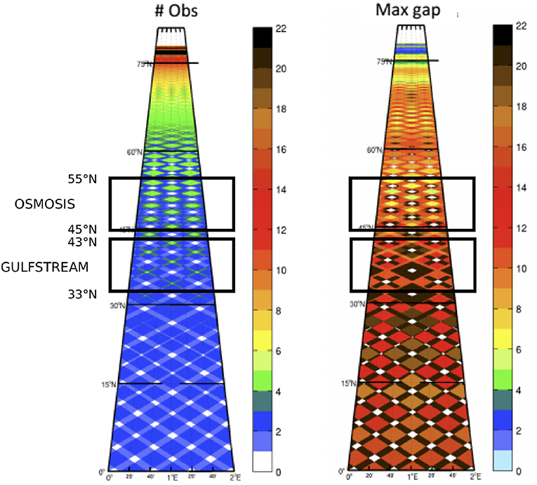
Figure 1. Figure from Ubelmann and Fu (personal communications) and from Vignudelli et al. (2019). Meridional distribution of the number of SWOT observations per satellite cycle (left) and distribution of the maximum gap in days between two consecutive SWOT observations (right). The black boxes have been added to illustrate the OSMOSIS and GULFSTREAM regions span over the latitude.

The paper is structured as follows. Section 2 recalls the errors expected to impact the SWOT data, describes the CER procedure from Metref et al. (2019) and provides the theoretical grounds to embed the CER in an ensemble-based DA scheme. Section 3 implements the DA with CER-data and tests it in the assimilation problem of SSH reconstruction using a one and a half layer QG model. Conclusions and perspectives are drawn in section 4.

2. Correlated-Error Reduced-Data Assimilation Method

2.1. SWOT Errors

The SWOT project team maintains a document describing the expected SWOT error budget (Esteban-Fernandez, 2017). The budget is made both in terms of spatial RMSE and wavenumber spectra, so that the SWOT mission is the first altimetric mission able to also set error requirements at different wavelengths. Indeed, standard SSH range errors have been given as a target for SWOT in the spatial domain and in the spectral domain (see Morrow et al., 2019, Figure 3). Based on this error budget, a simulator of SWOT-like observations was developed by the NASA Jet Propulsion Laboratory (Gaultier et al., 2016). This SWOT simulator allows the scientific community to produce artificial SWOT data for OSSE. The SWOT simulator interpolates any SSH simulation onto the SWOT swath groundtrack and computes and adds a realization of the SWOT errors. The SWOT simulator only generates the main SWOT errors described in Esteban-Fernandez (2017): Ka-Band Radar Interferometer (KaRIn) error, residual roll error, phase error, baseline dilation error, timing error, wet-troposphere error. Of those six errors, only four are concerned by the CER procedure. The KaRIn error is the instrumental random error, uncorrelated in space with a non-constant variance across track (see Appendix). This uncorrelated error is not taken into account in the procedure. However, uncorrelated errors are by construction well dealt with by the assimilation process, as confirmed by the results in section 3. The wet-troposphere error corresponds to the signal path delay due to the variability of the water vapor content in the troposphere. This delay introduces small scale isotropically correlated errors. In the CER formulation, we do not consider the wet-troposphere error as it has local across-track correlations that are smaller than the across-track swath and the method only deals with non-local across-track correlations that have specific geometries on the swath. Moreover, the wet-troposphere error is not expected to be the largest contributing error. However, combining the CER method with existing techniques for locally correlated errors (Brankart et al., 2009; Ruggiero et al., 2016; Yaremchuk et al., 2018) in order to take into account the wet-troposphere error should be investigated in future studies and should further improve the results. The four errors concerned by the reduction procedure are the timing error, the roll error, the baseline dilation error and the phase error. The timing error is only due, at first order, to a timing drift in the instrument signal propagation and can be assumed to be constant across track. The roll error is generated by the satellite roll angle, which impacts the measurement linearly across-track and is zero at its center. The baseline dilation error comes from the length variation of the satellite mast which creates a deviation between the two calibrated sensor signals. This creates a quadratic error distribution in the across-track direction. Finally, the phase error is due to the relative phase variations of the two sensors which produce cross-track linear errors independent in each half-swath. The across-track correlation structure of the four cumulated sources of error can be modeled by:

$\begin{array}{ll}{e}_{\text{total}}={\alpha }_0+{\alpha }_1{x}_c+{\alpha }_2{x}_c^2+\left[{\alpha }_3+{\alpha }_4{x}_c\right]{H}(-x_c)+\left[{\alpha }_5+{\alpha }_6{x}_c\right]{H}(x_c),& (1)\end{array}$

with x_c the across-track distance to the nadir, i.e., from −50 to −10 km and from 10 to 50 km; ${H}(x)$ the Heaviside function which equals 1 when x > 0 and 0 otherwise; and where {_{αi}i = 0, …, 6} are unknown constant coefficients. In Equation (1), the first term corresponds to the timing error, the second to the roll error, the third to the baseline dilation error and the last two terms correspond to the phase error in each half-swath.

Note that another source of error might indirectly impact the SWOT data. In order to be able to assimilate altimetric data in a model, the SSH must be converted to sea level anomalies by removing an estimated mean dynamic topography (MDT). An inaccurate MDT estimation could lead to additional SWOT errors. The estimation of MDT is a large field of investigation in itself and will not be addressed in this study. Here, we make the assumption of a perfect MDT and directly assimilate SSH. However, we believe that this issue should be independent enough to have no impact on the CER method tested here.

2.2. Correlated-Error Reduction Procedure

In order to remove the part of the SWOT signal h impacted by the errors, we first calculate the projection of h onto the subspace spanned by the modeled errors in Equation (1). This projection is performed by calculating the coefficients minimizing the following cost function:

$\begin{array}{l}J\left({\left\{{\alpha }_i\right\}}_{i=0,\mathrm{...},6}\right)={\displaystyle \sum _{x_c=-\frac{n_c}{2}}^{\frac{n_c}{2}}}(\overline{h}(x_c)-\{{\alpha }_0+{\alpha }_1{x}_c+{\alpha }_2{x}_c^2\\ +[{\alpha }_3+{\alpha }_4{x}_c]{H}(-x_c)+[{\alpha }_5+{\alpha }_6{x}_c]{H}(x_c)\}{)}^2,& (2)\end{array}$

with n_c the number of across track grid points and where $\bar{h}$ is the SWOT signal h averaged along-track on the region. Indeed, if the coefficients {_{αi}i = 0, …, 6} are not estimated accurately, the process could actually introduce artificial variations in the CER-data. Hence, similarly to Metref et al. (2019), in order to increase the accuracy of the coefficient estimation, we make the assumption that the coefficients are constant along-track over each pass. Further, we justify the small impact of this assumption by the relatively small size of the regions of interest GULFSTREAM and OSMOSIS. In other words, the scale of the along-track correlations of the errors considered in the reduction method is assumed larger than the size of the regions.

The CER-data is then defined as the residual between the SWOT signal h and the projection of $\bar{h}$:

$\begin{array}{l}T(h(x_c,x_a))=h(x_c,x_a)-\{{\alpha }_1{x}_c+{\alpha }_2{x}_c^2\\ +[{\alpha }_3+{\alpha }_4{x}_c]{H}(-x_c)+[{\alpha }_5+{\alpha }_6{x}_c]{H}(x_c)\},& (3)\end{array}$

for all across- and along-track grid points (x_c, x_a) and with {_{αi}i = 1, …, 6} the coefficients minimizing ${J}$ in Equation (2). Note that the constant term of the projection α₀ has to be removed from Equation (3) due to the fast variations of the timing error that are not in agreement with the constant projection in the along-track direction (more details in Metref et al., 2019).

2.3. Embedding the Correlated-Error Reduction Procedure in Data Assimilation

In the present paper, we make the case that the SWOT data h are too strongly affected by large and non-locally correlated errors to be directly assimilated in most operational systems. Indeed, the presence of correlated errors leads to non-diagonal observation error covariance matrices which most DA schemes need to invert. In large dimension, the cost of this inversion is too high for operational systems assimilating a large number of observations and, in practice, they commonly use diagonal matrices thus ignoring the error correlations. This approximation can no longer stand for the strongly spatially correlated SWOT errors. However, by construction and as shown in Metref et al. (2019), the SWOT CER-data ${T}$ have reduced correlations. Hence, in this paper, we propose to assimilate $h^{\text{o}}={T}(h)$ instead of h. In order to be consistent, it is important to realize that ${T}(h)$ is not a direct observation of SSH but a proxy. Therefore, the observation operator linking the model state to the observation must also include the CER procedure. If we note h^m the SSH described by the model and ${I}$ the interpolation from the model grid to the SWOT grid, the observation operator is now:

$\begin{array}{ll}H\equiv {T}◦{I}& (4)\end{array}$

and the innovation, i.e., the difference between the model state and the observation in the observation space, becomes $\left[h^{\text{o}}-{T}({I}(h^{\text{m}}))\right]$.

The CER procedure can be embedded in any DA method that uses the observation operator. Once the {_{αi}i = 1, …, 6} coefficients have been computed, ${T}$ is linear in h and it is possible to compute the adjoint observation operator for variational DA schemes, for instance. The algorithms for the CER of the SWOT data and for the embedding of the CER in the observation operator are summed up in Figure 2.

FIGURE 2

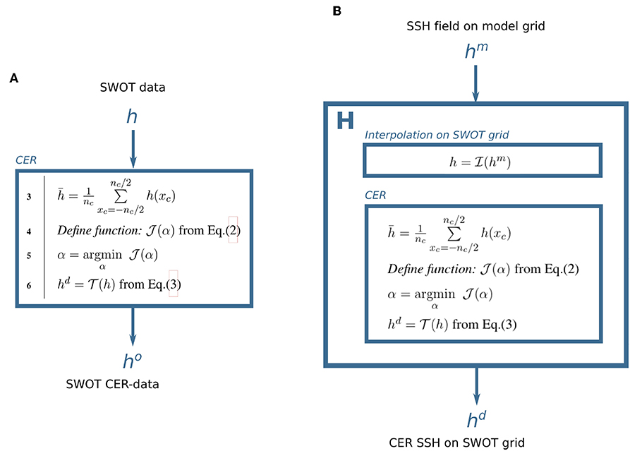
Figure 2. Algorithms for (A) the CER of the SWOT data and (B) the embedding of the CER in the observation operator H (see Equation 4).

In this study, we focus on ensemble-based DA. In particular, the numerical experiments presented in section 3 implement the CER procedure in an ensemble transform Kalman filter (ETKF). In practice, this implementation corresponds to N_e + 1 CERs at each analysis time step, where N_e is the number of ensemble members: N_e CERs for the ensemble and one CER for the SWOT data. Note that the computational cost for these N_e+1 operations remains small in comparison with the DA process itself.

3. Numerical Experiments

3.1. Experimental Setup

In the following OSSE, we consider the North Atlantic high resolution (1/60° at the Equator) numerical simulation (NATL60, 2018), generated with the NEMO model, as the true ocean. The NATL60 simulation has been used in several studies (Amores et al., 2018; Fresnay et al., 2018; Metref et al., 2019) and is one of the most advanced basin-scale high resolution simulations available to this day (approximately 10 km effective resolution).

The goal of this study is the evaluation of the CER-data in a DA problem cycled in time. The assimilation experiments start on October 1st, 2012 and end on December 31st, 2012. Only the last 2 months of the experiments are considered for the evaluation in order to let the DA processes converge, i.e., the diagnostics are performed from November 1st, 2012 to December 31st, 2012 (respectively referred to as t = 0 and t = 61 in Figures 6, 7). During these 2 months, the SWOT satellite almost completes three repeat cycles of the globe.

Figure 3 shows a snapshot of the SSH (in meters), in the two regions of interest: GULFSTREAM (left panel) and OSMOSIS (right panel), on November 4, 2012. The GULFSTREAM region is defined from 33 to 43°N in latitude and 53 to 65°W in longitude. The OSMOSIS region (defined from 45 to 55°N in latitude and 11 to 19°W in longitude) is part of the Porcupine Abyssal plain region and was intensively studied during the OSMOSIS campaign (Buckingham et al., 2016). The two regions differ in the intensity of their SSH variations. GULFSTREAM is zonally crossed by the Gulf Stream current which has a strong signature on SSH with heights reaching one meter. The OSMOSIS region rarely reaches 20 cm SSH but displays numerous small-scale eddies. Also, the difference in latitude between the regions impacts the frequency of observation by the SWOT satellite. The OSMOSIS region is at least partially observed every day while the GULFSTREAM region can be unobserved during 5 days straight. The two regions hence provide two distinct situations that SWOT will encounter.

FIGURE 3

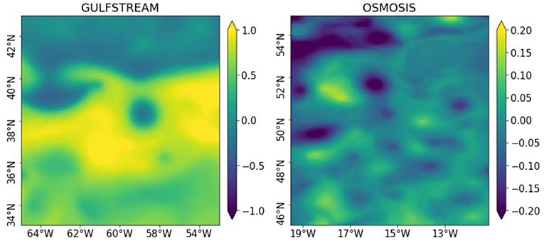
Figure 3. SSH fields (in meters), in the two regions of interest: GULFSTREAM (left) and OSMOSIS (right), on November 4, 2012.

From the “true ocean,” artificial SWOT data are created using the SWOT simulator (see Appendix A of Metref et al., 2019, for the detailed SWOT simulator parameters). The SWOT data were generated on the “Science orbit” which has a repeat cycle of approximately 21 days and corresponds to an orbital scenario of 77.6° inclination and 891 km elevation (SWOT simulator, 2016). Four DA experiments will be compared: (i) ETKF no error, which assimilates the SWOT data without error; (ii) ETKF KaRIn error, which assimilates the SWOT data with only the uncorrelated KaRIn error; (iii) ETKF full errors, which assimilates the SWOT data with all errors available on the simulator (see section 2.1); and (iv) ETKF reduced errors, which assimilates the SWOT CER-data.

The model used for SSH propagation is a one and a half layer QG model as described in Ubelmann et al. (2015). The QG model propagates the SSH by advecting the corresponding potential vorticity with the geostrophic currents. The first Rossby radius of deformation used are approximately 36 and 22 km in the GULFSTREAM and OSMOSIS region, respectively. The model time step is 10 min.

The DA scheme implemented is an ensemble transform Kalman filter with domain localization (Hunt et al., 2007). The DA localization function is $L(r)=e^{-r^2/L^2}{H}(R-r)$, for r the distance to the observation and where ${H}$ is the Heavyside function (see Equation 1). The localization radius L is set to 30 km and the localization cutoff R to 90 km. The codes for the DA scheme used in this study are available at SeSAM (2019). The filter is used sequentially with a 3 h cycle time step, i.e., an analysis is performed every 3 h if an observation is available in the region at that time. The filter runs with 50 ensemble members, which are initialized by randomly selecting NATL60 SSH fields between April and September 2013. An inflation of 1% is applied on the ensemble before every analysis for all assimilations. The observation error covariance matrix R is assumed diagonal for the four assimilations, as previously discussed. For the ETKF no error assimilation, R is prescribed constant along the diagonal of standard deviation 2 cm. The standard deviation is not set to 0 because the observation error covariance matrix represents the instrumental or measurement errors (which are not present in the ETKF no error experiment) but also the representativity errors. The SWOT grid is different from the model grid therefore an interpolation is performed by the observation operator H. This interpolation generates errors which are hard to quantify a priori. We have performed the ETKF no error experiment with various values of standard deviation on the diagonal observation error covariance matrix and we have selected the one providing the smallest RMSE which is a 2 cm standard deviation. For the ETKF KaRIn error assimilation, R is prescribed with the error standard deviations used to create the KaRIn error (see Appendix). The ETKF full errors and ETKF reduced errors assimilations use the same matrix R as the ETKF KaRIn error assimilation but with an inflation of 30 and 10%, respectively in GULFSTREAM and of 40 and 20%, respectively in OSMOSIS. These inflation coefficients were manually tuned to provide the smallest SSH RMSE (not shown here). The ETKF reduced errors needs less inflation because the CER method reduces the non-local correlations. However, it does not remove them entirely so that some inflation is still needed.

3.2. Results

Figures 4, 5 display, in GULFSTREAM and OSMOSIS, respectively, the SSH reconstructions (left columns) obtained with the four assimilations corresponding to the true SSH fields in Figure 3. The right columns of Figures 4, 5 are the point-wise differences with the true SSH fields. These fields correspond to November 4, 2012, more than a month after the beginning of the assimilation processes. In GULFSTREAM, a SWOT pass has just been assimilated which explains the white track on the right of the panels corresponding to the local analysis of the ETKF. In OSMOSIS, no analysis was recently performed at day November 4, 2012 but the error across-track variations of previous observations that were forecast remain visible in the ETKF full errors reconstruction. This confirms the importance of assessing the impact of the SWOT errors and the CER-data in an assimilation problem cycled in time.

FIGURE 4

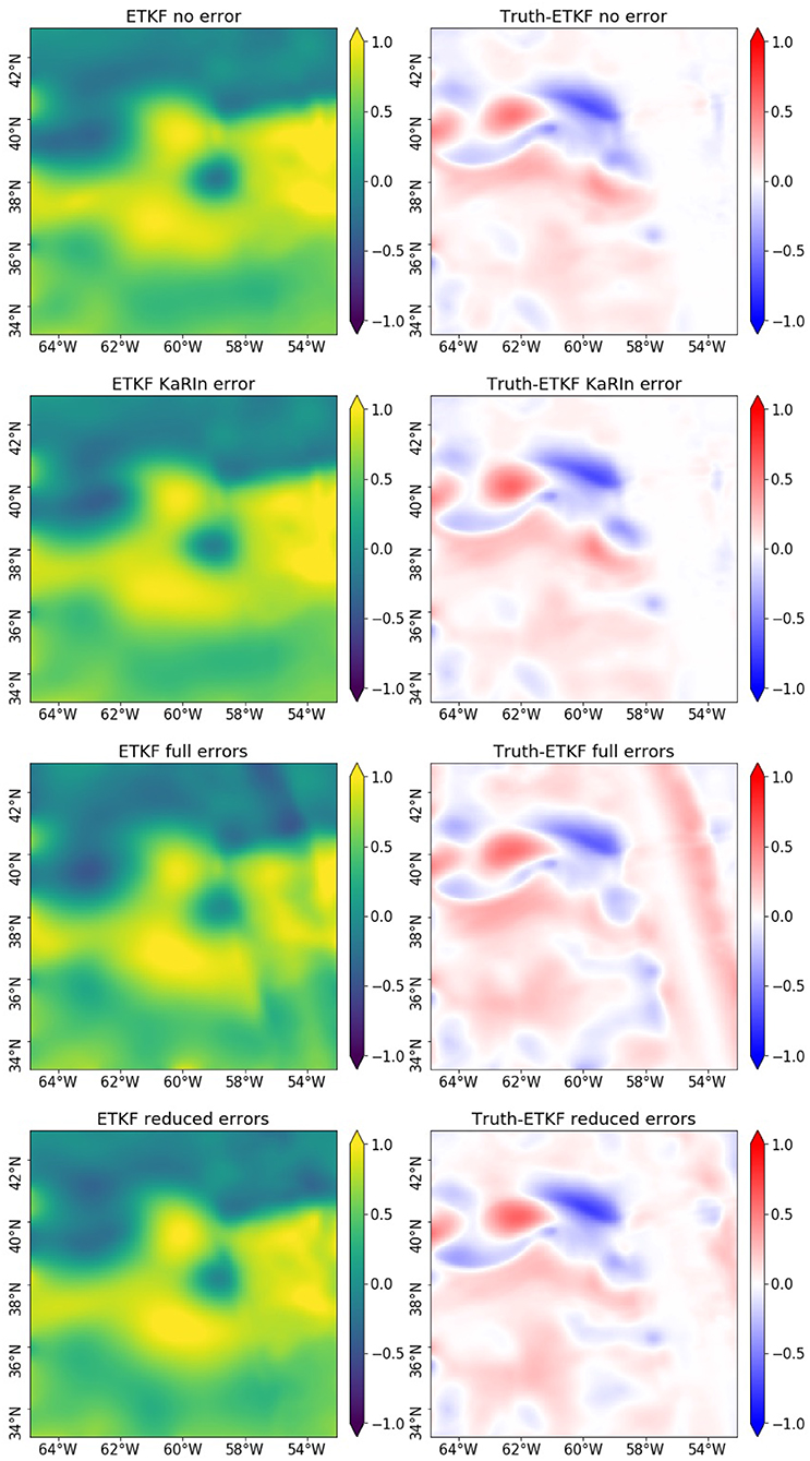
Figure 4. SSH (in meters) field reconstructions (left column), in GULFSTREAM, performed by the four assimilations and their differences (right column) to the true state on November 4, 2012 displayed in Figure 3.

FIGURE 5

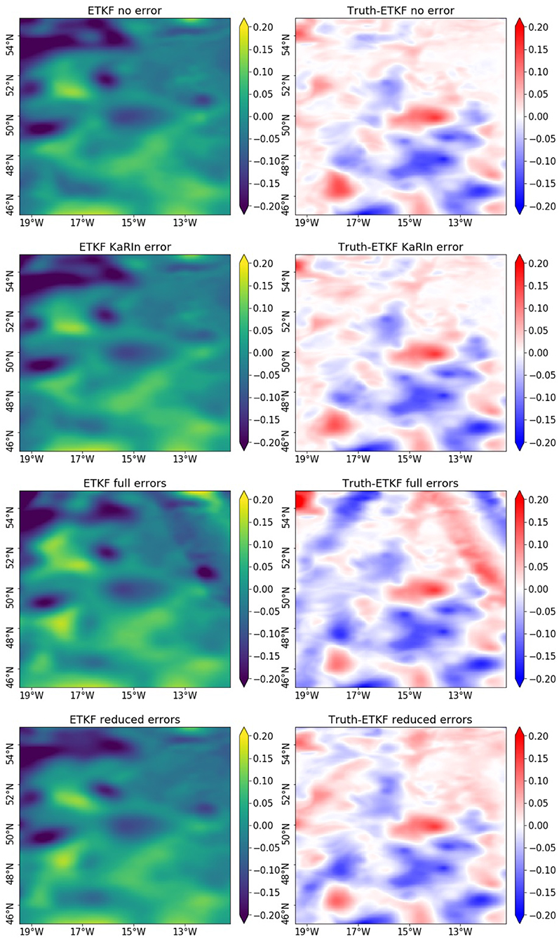
Figure 5. Same as Figure 4 but in OSMOSIS.

The first result is that the reconstruction produced by the assimilation without error and with the KaRIn error only are very similar. This indicates that, as expected, the ETKF seems well-suited to deal with the uncorrelated KaRIn error. However, in both GULFSTREAM and OSMOSIS cases, the ETKF assimilating the full errors is very much affected by the spatially correlated errors. As previously mentioned, in both cases, the satellite tracks and the error across-track variations impact the reconstructions. This is particularly visible on the recently assimilated SWOT track on the right of the panels in GULFSTREAM, where a large error across-track variation appears in the ETKF full errors reconstruction. The CER does not entirely remove the spatially correlated errors impact but strongly reduces it. Unlike the SSH fields reconstructed by ETKF full errors, the fields reconstructed by ETKF reduced errors seem geophysical, visually at least, in the sense that there are no unrealistic strong gradients or discontinuities in the SSH.

In order to quantify the improvement brought by the CER-data, we compute the RMSE of the SSH reconstructed fields at each time to obtain RMSE time series. The RMSE of a 2D reconstructed field x = {x}_{i = 1, …N} with respect to the true field ${\text{x}}^{\text{t}}={\left\{x^{\text{t}}\right\}}_{i=1,\dots N}$ is calculated as such:

$\begin{array}{ll}\text{RMSE}(\text{x})=\sqrt{\frac{1}{N}{\displaystyle \sum _{i=1}^N}{(x_i-x_i^{\text{t}})}^2}& (5)\end{array}$

with N the number of grid points. Figure 6 shows the RMSE time series calculated in GULFSTREAM during the 2 month experiment for the SSH, the relative vorticity ζ and the currents (u, v). The RMSE show the cycles of the SWOT track crossing the GULFSTREAM region with approximately 9 day periods when the region is well-observed and 5 day periods with almost no observation in the region. In this configuration, it is interesting to note that during the forecasting periods (i.e., when there is no available observation), all the DA experiments deviate quickly from the truth which is due to the idealistic QG model used for the propagation. The first important result of these experiments is the very close RMSE on all four variables produced by the assimilation of the error-free SWOT data and the KaRIn error only SWOT data. This means that in terms of RMSE the KaRIn error is being well delt with by the ETKF assimilation scheme. During the time periods without observation, ETKF full errors and ETKF reduced errors assimilations have approximately the same errors. Figure 6 also shows that, after a 6 day period without observation, the ETKF reduced errors can sometime produce more inaccurate SSH fields than ETKF full errors. If this behavior persists in a more realistic setting, this could be problematic when using SWOT to initialize a long forecasting phase. This result should be further investigated in future studies. However, when the region is well-observed, using the CER-data helps reduce the RMSE. At day 39, for instance, the SSH RMSE of the ETKF reduced errors is half the one of the ETKF full errors. The RMSE on average over the 2 month experiment are listed in Table 1. The averaged RMSE confirm the improvement brought by the CER-data. Indeed, in GULFSTREAM, the averaged SSH RMSE of the reconstruction is 9.3 cm without error, 12.1 cm with full errors, but is reduced to 10.9 cm by the CER, i.e., a 10% RMSE reduction. Similarly, on the relative vorticity and on the surface currents, the RMSE reduction is between 5 and 10% when using the CER method. In OSMOSIS, because of the smaller magnitude of the SSH variations, the impact of the SWOT errors on the reconstruction in that region is very substantial. Figure 7 shows the large benefit of using the CER-data in the OSMOSIS region with, at day 15 for example, an SSH RMSE reduction of over 60%, and on average (see Table 1) the SSH RMSE reduction is around 45%.

FIGURE 6

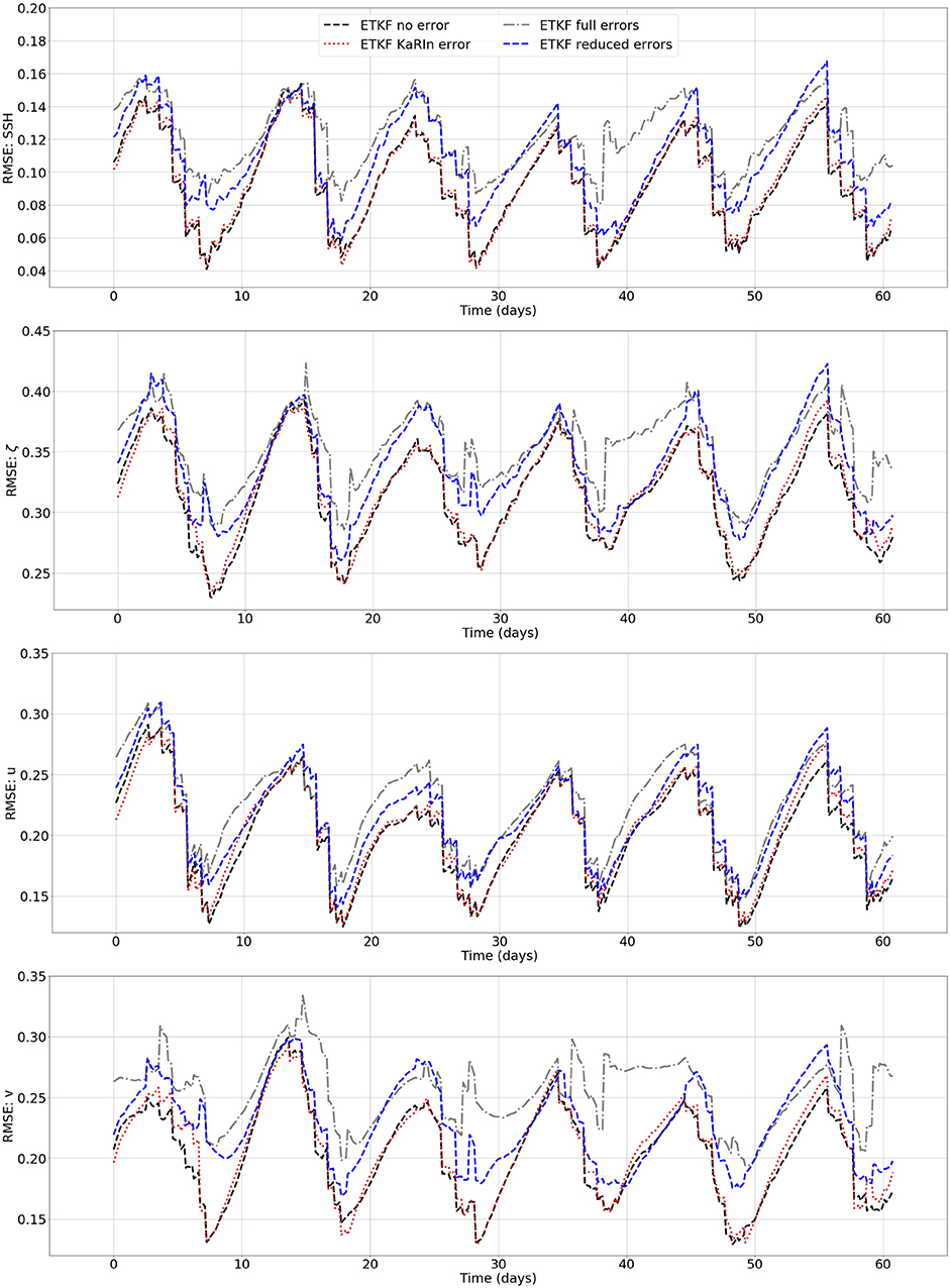
Figure 6. RMSE time series for the four assimilations during the 2 month experiment in GULFSTREAM for SSH (in meters, first line), ζ (adimensional, second line), u (in m/s, third line), and v (in m/s, fourth line).

TABLE 1

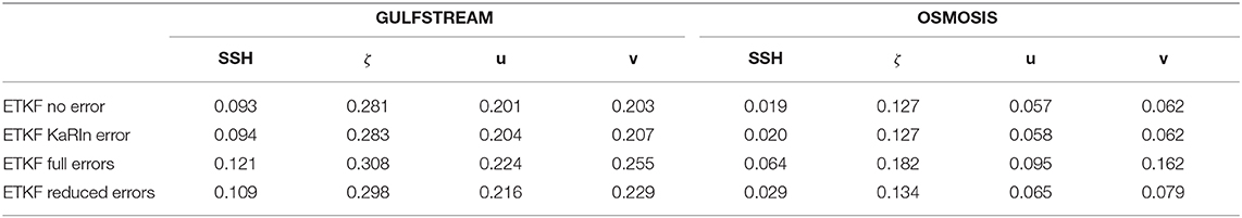
Table 1. RMSE averaged over the 2 month experiment for the four assimilations in GULFSTREAM and OSMOSIS for SSH (in meters), ζ (adimensional), u (in m/s), and v (in m/s).

FIGURE 7

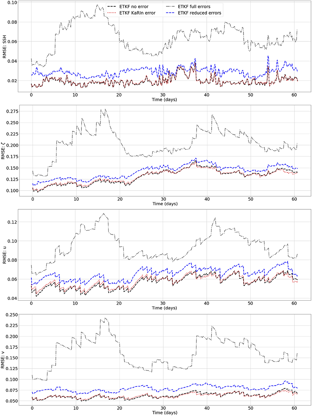
Figure 7. Same as Figure 6 but in OSMOSIS.

As mentioned in section 2.1, the SWOT errors were designed to respect error specifications in the spectral domain, however, the RMSE does not allow to assess the reconstructions independently in the different spatial scales. Moreover, the SWOT mission objectives were defined in terms of spectra, with a resolution on the swath of 15–30 km (Morrow et al., 2019). Hence, it is necessary to assess the impact of the full SWOT errors on the small scales. Here, we perform three two-dimensional spectral diagnostics on the SSH: the power spectral density, the noise-to-signal ratio and the spectral coherence. The power spectral density (PSD) is a 2D wavenumber spectrum which describes the energy of the signal at the different spatial scales. In order to compute this two-dimensional PSD (described in more details by Ajayi et al., 2019), a two-dimensional fast Fourier transform (FFT) is applied to the SSH fields (after removing the linear biases, in both latitude and longitude directions, and tapering the data using a Tukey window). We then average this 2D FFT in the azimuthal direction to obtain a one-dimensional isotropic spectrum. The noise-to-signal ratio NSR (Ballarotta et al., 2019) compares an estimated signal x to a true signal x^t such that:

$\begin{array}{ll}\text{NSR}(\text{x})=1-\frac{PSD(\text{x}-{\text{x}}^{\text{t}})}{PSD({\text{x}}^{\text{t}})}.& (6)\end{array}$

When the energy of the residual x − x^t is small compared with the energy of the true signal x^t, the NSR should be close to 1. And finally, the spectral coherence is the square of the cross-spectral density between two signals divided by the product of the autospectral densities of both signals and describes the spatial correlations between the signals (here, the estimated signal and the true signal) at the different scales. The spectral coherence should be also close to 1 if the estimated signal and the true signal are strongly correlated. The numerical codes used to compute all the spectral diagnosis described above are available online at PowerSpec (2019). Figure 8 shows these three diagnostics, averaged over the 2 month experiment, for the four assimilations in GULFSTREAM (left column) and in OSMOSIS (right column). The PSD show very similar energy reconstruction at large scales for ETKF no error and ETKF KaRIn error in both regions which is consistent with the previous RMSE results. Also, the noise-to-signal ratio and the spectral coherence remain unaffected by the KaRIn error. However, the PSD also show that the KaRIn error degrades the small scale energy reconstruction, especially in the low energy region OSMOSIS. In fact, ensemble Kalman filters in general are known to focus on the large scales and underperform in the small scales as they are based on a finite number of ensemble members. Hence, this result suggests that a pretreatment of the SWOT data to reduce the KaRIn error before assimilation may help. In GULFSTREAM, the spatially correlated errors do not seem to have a significant impact on the reconstruction in terms of spectral diagnostics, especially for the PSD. This is probably due to the averaging over the 2 month experiment in a very energetic region. Nonetheless, a slight improvement made by the DA with CER-data can be seen in terms of noise-to-signal ratio NSR and spectral coherence at mesoscale (100–200 km) but with also, a slight degradation at large scales (>300 km). In OSMOSIS, on the other hand, the full errors strongly impact the energy reconstruction at large scales. And, even if the spectral coherence is around 0.6 in the large scales the noise-to-signal ratio shows that the PSD of the residual (i.e., estimate minus truth) is larger than the PSD of the truth, resulting in a negative noise-to-signal ratio. The DA with CER-data restores a well estimated energy at large scales and significantly increases the noise-to-signal ratio and spectral coherence at all scales.

FIGURE 8

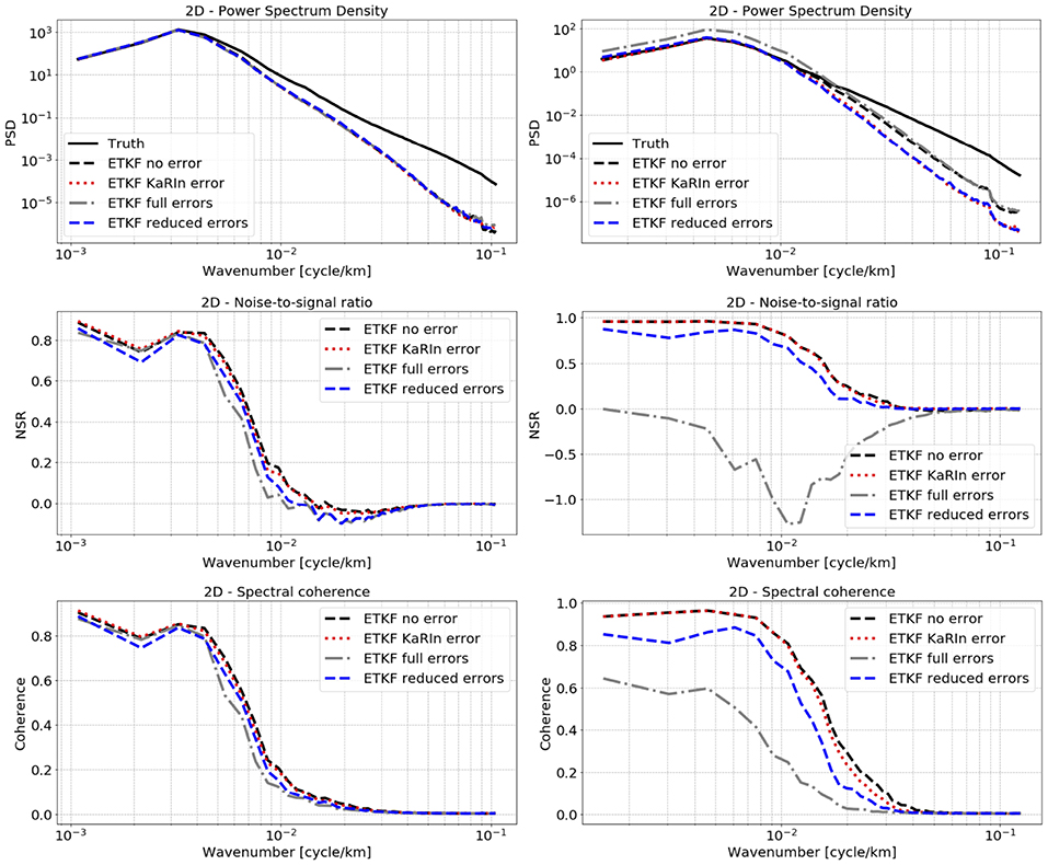
Figure 8. Power spectral density in m²/cycle/km (first line), noise-to-signal ratio (second line), and spectral coherence (third line) on SSH, for the four assimilations, averaged during the 2 month experiment in GULFSTREAM (left column) and OSMOSIS (right column).

In a nutshell, the spectral diagnostics confirm that the GULFSTREAM region is less impacted by the SWOT full errors than OSMOSIS which is explained by the large SSH variability in comparison to the error variability and by the lower observation frequency in GULFSTREAM. Also, in terms of energy reconstruction, the PSD show that DA with CER-data removes the impact of the correlated errors on the energy of the reconstructed signal. The only difference left between the ETKF reduced errors and the ETKF no error can be explained by the impact of the KaRIn error on the small scales and the inability of the ETKF to deal with them. Finally, in terms of noise-to-signal ratio and spectral coherence, the full errors strongly degrade the reconstruction at all scales in OSMOSIS. The reconstruction with the CER procedure does not produce a signal as coherent as the one produced by the ETKF no errors, but manages to strongly improve the reconstruction from the large scales down to between 100 and 50 km. In GULFSTREAM, however, the full errors are small relative to the SSH signal and, in this case, the CER procedure causes degradation at scales over 300 km.

4. Conclusions

The goal of this study was to assess the embedding of the correlated-error reduction (CER) procedure proposed by Metref et al. (2019) in an ensemble-based data assimilation (DA) scheme in order to better assimilate the SWOT data with spatially correlated errors. The assimilation problem proposed for that assessment was an OSSE for SSH field reconstruction using a one and a half layer QG model in two different regions: GULFSTREAM (defined from 33 to 43°N and from 53 to 65°) and OSMOSIS (defined from 45 to 55°N and from 11 to 19°W). By comparing ETKF assimilations of: (i) the error-free SWOT data, (ii) the KaRIn error SWOT data, (iii) the SWOT data with full errors; and (iv) the SWOT correlated-error reduced-data (CER-data), the study has reached three major results.

The first major result is not directly related to the CER-data assessed in this experiment but is a first answer to one of the major questions in the SWOT community (Rodriguez et al., 2017; Chelton et al., 2019; Morrow et al., 2019) about the impact of the KaRIn error on SWOT DA. We have shown that, when assimilating SWOT data with an ETKF, the presence of KaRIn error does not have a significant effect on the SSH, the relative vorticity, and the currents neither in terms of RMSE nor in terms of noise-to-signal ratio and spectral coherence. However, the presence of KaRIn error slightly dampens the energy at small scales (under 200 km in GULFSTREAM and below 100 km in OSMOSIS). This result suggests that a pretreatment of the SWOT data to reduce the KaRIn error would help provide a better resolution of SWOT DA reconstructions in terms of energy.

The second major result is that, in strongly energetic and less frequently observed regions such as GULFSTREAM, the DA with CER-data manages to reduce the SSH RMSE by 10% on average. The RMSE of relative vorticity and currents are also reduced by between 5 and 10%. Nevertheless, the DA with CER-data can sometimes slightly degrade the solution after a 6 day period without observation. This limitation may be due to the use of an idealistic model in this study and should be investigated in a more realistic setting in future works. During an intensely observed time period, however, the experiments showed that DA with CER-data can reduce the SSH RMSE by up to 50%. This result shows that using CER-data could be of crucial importance during the fast sampling phase of SWOT where the satellite will have a 1 day revisit time and several regions of the globe will be intensively observed. The energy distribution throughout the spatial scales does not seem to be impacted by the spatially correlated errors. The DA with CER-data slightly improves the noise-to-signal ratio and spectral coherence at mesoscale (100–200 km). However, the method also slightly degrades the noise-to-signal ratio and spectral coherence at large scales (>300 km).

Finally, the third major result is the importance of assimilating a SWOT CER-data in less energetic regions such as OSMOSIS. The average SSH RMSE are more than halved when assimilating the CER-data rather than the raw data and the RMSE of relative vorticity and currents are significantly reduced as well. The signal energy at large and meso-scales is very well-estimated and the noise-to-signal ratio and spectral coherence are much improved by the DA with CER-data from the large scales down to small mesoscale (between 100 and 50 km).

The study presented here was an OSSE that focused on the effects of the SWOT errors on the assimilation in the ocean surface using a QG model and the improvements brought by the CER-data. The possible limitations of this study are that (i) the OSSE experiments were based on simulations without internal tides which would further complexify the SSH signals, (ii) the DA experiments only targeted the reconstruction of surface fields, (iii) the assimilation system used a QG propagator which does not account for some aspects of the dynamics of oceanic flows at fine scale (intense ageostrophic flows at submesoscale fronts and internal waves). Future works should expand this study by implementing a more complex assimilation system and assess the benefits of DA with CER-data on the vertical dimension of the ocean. Also, as already stated in Metref et al. (2019), the CER should be tested in larger regions with an adaptative computation in the along-track direction. Finally, as part of a larger challenge mobilizing the SWOT community, it will be crucial to investigate the behavior of the CER-data methodology in the presence of internal tides.

Data Availability Statement

The datasets generated for this study are available on request to the corresponding author.

Author Contributions

SM, EC, and JL designed the study. SM, EC, JL, and J-MB designed the numerical experiments. FL contributed to the implementation tools for the SWOT assimilation. SM, EC, JL, and FL contributed to the analysis of the results. SM led the redaction of the manuscript and all authors contributed to the writing.

Funding

This research was funded by ANR (project number ANR-17-CE01-0009-01) and CNES through the OST/ST and the SWOT Science Team.

Conflict of Interest

The authors declare that the research was conducted in the absence of any commercial or financial relationships that could be construed as a potential conflict of interest.

Acknowledgments

The authors thank Maxime Ballarotta and Clément Ubelmann from CLS and Lee-Lueng Fu from the Jet Propulsion Laboratory for the constructive discussions related to this study.

References

Ajayi, A., Sommer, J. L., Chassignet, E., Molines, J.-M., Xu, X., Albert, A., et al. (2019). Diagnosing cross-scale kinetic energy exchanges from two submesoscale permitting ocean models. Earth Space Sci. Open Archive. doi: 10.1002/essoar.10501077.1. [Epub ahead of print].

CrossRef Full Text | Google Scholar

Amores, A., Jordà, G., Arsouze, T., and Le Sommer, J. (2018). Up to what extent can we characterize ocean eddies using present-day gridded altimetric products? J. Geophys. Res. 123, 7220–7236. doi: 10.1029/2018JC014140

CrossRef Full Text | Google Scholar

Ballarotta, M., Ubelmann, C., Pujol, M.-I., Taburet, G., Fournier, F., Legeais, J.-F., et al. (2019). On the resolutions of ocean altimetry maps. Ocean Sci. 15, 1091–1109. doi: 10.5194/os-15-1091-2019

CrossRef Full Text | Google Scholar

Brankart, J.-M., Ubelmann, C., Testut, C.-E., Cosme, E., Brasseur, P., and Verron, J. (2009). Efficient parameterization of the observation error covariance matrix for square root or ensemble kalman filters: application to ocean altimetry. Monthly Weather Rev. 137, 1908–1927. doi: 10.1175/2008MWR2693.1

CrossRef Full Text | Google Scholar

Buckingham, C. E., Naveira Garabato, A. C., Thompson, A. F., Brannigan, L., Lazar, A., Marshall, D. P., et al. (2016). Seasonality of submesoscale flows in the ocean surface boundary layer. Geophys. Res. Lett. 43, 2118–2126. doi: 10.1002/2016GL068009

CrossRef Full Text | Google Scholar

Chelton, D. B., Ries, J. C., Haines, B. J., Fu, L.-L., and Callahan, P. S. (2001). “Chapter 1: Satellite altimetry,” in Satellite Altimetry and Earth Sciences, Volume 69 of International Geophysics, eds L. L. Fu and A. Cazenave (San Diego, CA: Academic Press), 1–2.

Google Scholar

Chelton, D. B., Schlax, M. G., Samelson, R. M., Farrar, J. T., Molemaker, M. J., McWilliams, J. C., et al. (2019). Prospects for future satellite estimation of small-scale variability of ocean surface velocity and vorticity. Prog. Oceanogr. 173, 256–350. doi: 10.1016/j.pocean.2018.10.012

CrossRef Full Text | Google Scholar

Esteban-Fernandez, D. (2017). Swot Project: Mission Performance and Error Budget. Revision A. Jet Propulsion Laboratory Doc., JPL D-79084.

Google Scholar

Fresnay, S., Ponte, A. L., Le Gentil, S., and Le Sommer, J. (2018). Reconstruction of the 3-D dynamics from surface variables in a high-resolution simulation of north atlantic. J. Geophys. Res. 123, 1612–1630. doi: 10.1002/2017JC013400

CrossRef Full Text | Google Scholar

Fu, L.-L., and Cazenave, A., . (eds.) (2001). Satellite Altimetry and Earth Sciences: A Handbook of Techniques and Applications, Volume 69. San Diego, CA: Elsevier.

Google Scholar

Fu, L.-L., and Chelton, D. B. (2001). “Chapter 2: Large-scale ocean circulation,” in Satellite Altimetry and Earth Sciences, Vol. 69 of International Geophysics, eds L. L. Fu and A. Cazenave (San Diego, CA: Academic Press), 133–viii.

Google Scholar

Gaultier, L., Ubelmann, C., and Fu, L.-L. (2016). The challenge of using future swot data for oceanic field reconstruction. J. Atmos. Ocean. Technol. 33, 119–126. doi: 10.1175/JTECH-D-15-0160.1

CrossRef Full Text | Google Scholar

Guillet, O., Weaver, A. T., Vasseur, X., Michel, Y., Gratton, S., and Grol, S. (2019). Modelling spatially correlated observation errors in variational data assimilation using a diffusion operator on an unstructured mesh. Q. J. R. Meteorol. Soc. 145, 1947–1967. doi: 10.1002/qj.3537

CrossRef Full Text | Google Scholar

Hunt, B. R., Kostelich, E. J., and Szunyogh, I. (2007). Efficient data assimilation for spatiotemporal chaos: a local ensemble transform kalman filter. Phys. D 230, 112–126. doi: 10.1016/j.physd.2006.11.008

CrossRef Full Text | Google Scholar

Janjić, T., Bormann, N., Bocquet, M., Carton, J. A., Cohn, S. E., Dance, S. L., et al. (2018). On the representation error in data assimilation. Q. J. R. Meteorol. Soc. 144, 1257–1278. doi: 10.1002/qj.3130

CrossRef Full Text | Google Scholar

Liu, Z.-Q., and Rabier, F. (2002). The interaction between model resolution, observation resolution and observation density in data assimilation: a one-dimensional study. Q. J. R. Meteorol. Soc. 128, 1367–1386. doi: 10.1256/003590002320373337

CrossRef Full Text | Google Scholar

Madec, G. (2015). “Nemo ocean engine,” in Note du Pôle de Modélisation; No 27; Institut Pierre-Simon Laplace (IPSL) (Paris), 343–367.

Google Scholar

Metref, S., Cosme, E., Le Sommer, J., Poel, N., Brankart, J.-M., Verron, J., et al. (2019). Reduction of spatially structured errors in wide-swath altimetric satellite data using data assimilation. Remote Sens. 11:1336. doi: 10.3390/rs11111336

CrossRef Full Text | Google Scholar

Miyoshi, T., Kalnay, E., and Li, H. (2013). Estimating and including observation-error correlations in data assimilation. Inverse Probl. Sci. Eng. 21, 387–398. doi: 10.1080/17415977.2012.712527

CrossRef Full Text | Google Scholar

Morrow, R., Fu, L.-L., Ardhuin, F., Benkiran, M., Chapron, B., Cosme, E., et al. (2019). Global observations of fine-scale ocean surface topography with the surface water and ocean topography (swot) mission. Front. Mar. Sci. 6:232. doi: 10.3389/fmars.2019.00232

CrossRef Full Text | Google Scholar

Morrow, R., and Le Traon, P.-Y. (2012). Recent advances in observing mesoscale ocean dynamics with satellite altimetry. Adv. Space Res. 50, 1062–1076. doi: 10.1016/j.asr.2011.09.033

CrossRef Full Text | Google Scholar

NATL60 (2018). meom-Configurations/NATL60-CJM165: NATL60 Code Used for CJM165 Experiment (Version v_1.0.0). Zenodo: doi: 10.5281/zenodo.1210116

CrossRef Full Text | Google Scholar

Oke, P. R., Brassington, G. B., Griffin, D. A., and Schiller, A. (2008). The bluelink ocean data assimilation system (bodas). Ocean Model. 21, 46–70. doi: 10.1016/j.ocemod.2007.11.002

CrossRef Full Text | Google Scholar

PowerSpec (2019). PowerSpec Python Package for Spectral Analysis of Two-Dimensional Oceanic Dataset. Available online at: https://github.com/adeajayi-kunle/powerspec

Google Scholar

Rodriguez, E., Fernandez, D. E., Peral, E., Chen, C. W., De Bleser, J.-W., and Williams, B. (2017). “Wide-swath altimetry: a review,” in Satellite Altimetry Over Oceans and Land Surfaces, eds D. Stammer and A. Cazenave (Boca Raton, FL: CRC Press), 71–112.

Google Scholar

Ruggiero, G. A., Cosme, E., Brankart, J.-M., Le Sommer, J., and Ubelmann, C. (2016). An efficient way to account for observation error correlations in the assimilation of data from the future swot high-resolution altimeter mission. J. Atmos. Ocean. Technol. 33, 2755–2768. doi: 10.1175/JTECH-D-16-0048.1

CrossRef Full Text | Google Scholar

SeSAM (2019). System of Sequential Assimilation Modules. Available online at: https://github.com/brankart/sesam

Google Scholar

Stammer, D., and Cazenave, A., (eds.). (2017). Satellite Altimetry Over Oceans and Land Surfaces. Boca Raton, FL: CRC Press.

Google Scholar

Stewart, L. M., Dance, S. L., and Nichols, N. K. (2008). Correlated observation errors in data assimilation. Int. J. Numer. Methods Fluids 56, 1521–1527. doi: 10.1002/fld.1636

CrossRef Full Text | Google Scholar

Stewart, L. M., Dance, S. L., and Nichols, N. K. (2013). Data assimilation with correlated observation errors: experiments with a 1-D shallow water model. Tellus A Dyn. Meteorol. Oceanogr. 65:19546. doi: 10.3402/tellusa.v65i0.19546

CrossRef Full Text | Google Scholar

SWOT simulator (2016). Ocean SWOT Simulator. Jet Propulsion Laboratory. Available online at: https://github.com/swotsimulator

Google Scholar

Ubelmann, C., Klein, P., and Fu, L.-L. (2015). Dynamic interpolation of sea surface height and potential applications for future high-resolution altimetry mapping. J. Atmos. Ocean. Technol. 32, 177–184. doi: 10.1175/JTECH-D-14-00152.1

CrossRef Full Text | Google Scholar

Vignudelli, S., Birol, F., Benveniste, J., Fu, L.-L., Picot, N., Raynal, M., et al. (2019). Satellite altimetry measurements of sea level in the coastal zone. Surveys Geophys. 40, 1319–1349. doi: 10.1007/s10712-019-09569-1

CrossRef Full Text | Google Scholar

Waller, J. A., Dance, S. L., Lawless, A. S., and Nichols, N. K. (2014). Estimating correlated observation error statistics using an ensemble transform kalman filter. Tellus A Dyn. Meteorol. Oceanogr. 66:23294. doi: 10.3402/tellusa.v66.23294

CrossRef Full Text | Google Scholar

Yaremchuk, M., D'Addezio, J. M., Panteleev, G., and Jacobs, G. (2018). On the approximation of the inverse error covariances of high-resolution satellite altimetry data. Q. J. R. Meteorol. Soc. 144, 1995–2000. doi: 10.1002/qj.3336

CrossRef Full Text | Google Scholar

Appendix

The KaRIn instrumental error is simulated by the SWOT simulator (2016) as an uncorrelated zero-centered Gaussian noise of standard deviation dependent on the distance with the nadir. The standard deviation of the KaRIn error is also dependent on the significant wave height (SWH) parameter which is a value between 0 and 8 m. Figure A1 represents the standard deviation with respect to the distance with the nadir (in one half-swath only) and for different SWH parameters. The KaRIn error used in the present study was produced with the parameter SWH = 2 m corresponding to the dark blue curve in Figure A1. As discussed in section 3.1, this standard deviation was also used to prescribe the diagonal observation error covariance matrix R for the assimilation ETKF KaRIn error (directly) and for the assimilations ETKF full errors and ETKF reduced errors (after inflation, see section 3.1).

FIGURE A1

Figure A1. Figure extracted from the SWOT simulator (2016) manual. The example curves of the standard deviation (cm) of the KaRIn errors as a function of cross-track distance (km).