Environmental Drivers of Seabird At-Sea Distribution in the Eastern South Pacific Ocean: Assemblage Composition Across a Longitudinal Productivity Gradient

Introduction

As marine top predators, seabirds respond to changes in the oceanography, ocean productivity, and their lower trophic-level prey (i.e., zooplankton, squid, and fish), shifting their distributions over multiple temporal scales (i.e., seasonally, inter-annually). Thus, groups of species with similar requirements may exhibit similar distribution patterns, forming assemblages that co-exist in space. To date, these biogeographic patterns have been characterized in some regions, like the South Pacific (Ainley and Boekelheide, 1983), the Eastern Tropical Pacific (Ballance et al., 1997), the North Pacific/Pacific Arctic Ocean (Piatt and Springer, 2003; Santora et al., 2017; Sigler et al., 2017), the Southern Indian Ocean (Hyrenbach et al., 2007), and the South Atlantic (Veit, 1995). However, despite the progress describing seabird distributions globally, we still lack a mechanistic understanding of how these patterns are generated (Ainley et al., 2012). Therefore, documenting these patterns and investigating their environmental drivers are critical steps toward understanding the macro-ecology of seabirds and their role in marine ecosystems. Moreover, this information has important conservation and ecosystem management implications globally, since the forecasted environmental changes are expected to affect the physical structure and productivity of the marine environment, and disrupt biotic communities (Polovina et al., 2008; Proud et al., 2017). However, to date, most studies have focused on habitat relationships of individual species, with few aiming to characterize how entire seabird assemblages are distributed over biogeographical scales and respond to environmental gradients.

Over macro-scales (i.e., 1000 km), seabirds respond to changing hydrographic properties, suggesting that specific assemblages are associated with the specific physical and biological characteristics of certain water masses (Ashmole, 1971; Hunt and Schneider, 1987). For example, seabird assemblages vary in response to changes in sea surface water temperature and salinity (Pocklington, 1979; Ainley and Boekelheide, 1983; Wahl et al., 1989; Force et al., 2015). In contrast, studies conducted in high latitude systems (e.g., the Antarctic and the Artic) highlight the important role of sea ice cover structuring the marine avifauna, with the presence of unique “ice-associated” assemblages (Ainley et al., 1993; Commins et al., 2014; Renner et al., 2016).

Other environmental drivers influence seabird assemblages over meso-scales (i.e., 100 km), with bathymetry, and seasonal changes in hydrography playing a key role, especially in broad continental shelves (Veit, 1995; Hunt et al., 2014; Santora et al., 2017). In addition to bathymetric gradients (i.e., the shelf-break), the boundaries between water masses with different productivity, temperature, density, or velocity (i.e., frontal zones) greatly influence species distributions at these spatial scales. In particular, these hydrographic features can act as biogeographic boundaries, affecting the overall seabird abundance and species richness (Scales et al., 2014). For instance, the tropical and subtropical transition front conspicuously delineates seabird distributions in the South Pacific (Ainley and Boekelheide, 1983) and the South Atlantic (Commins et al., 2014). Moreover, in the Southern Ocean, the Polar Front delineates the distribution of distinct latitudinal seabird assemblages and enhances the abundance of certain species that forage at the front (Bost et al., 2009; Force et al., 2015). While this evidence underscores the influence of hydrography on the distribution and abundance of seabirds, major areas of the global ocean have not been surveyed and characterized.

Macro-scale studies of seabird assemblages in the Eastern South Pacific Ocean (ESPO) have been restricted to the southern tip of South America and the Humboldt Current (Jehl, 1973; Brown et al., 1975; Weichler et al., 2004; Spear and Ainley, 2008). Thus, there is a lack of knowledge regarding seabird distributions farther west, between the west coast of South America and the eastern limit of the South Pacific Gyre (Figure 1) (but see Miranda-Urbina et al., 2015). This area provides a great natural experiment to examine the environmental factors driving seabird distributions, because it encompasses a strong gradient in primary productivity, and water mass properties (temperature and salinity). This gradient extends from the low temperature and low salinity water of the Humboldt Current to the East, which constitutes one of the most productive systems of the world, to the high temperature and high salinity waters of the South Pacific Gyre to the West, which is the largest low-productivity domain in the world (Longhurst, 2007; Morel et al., 2010).

FIGURE 1

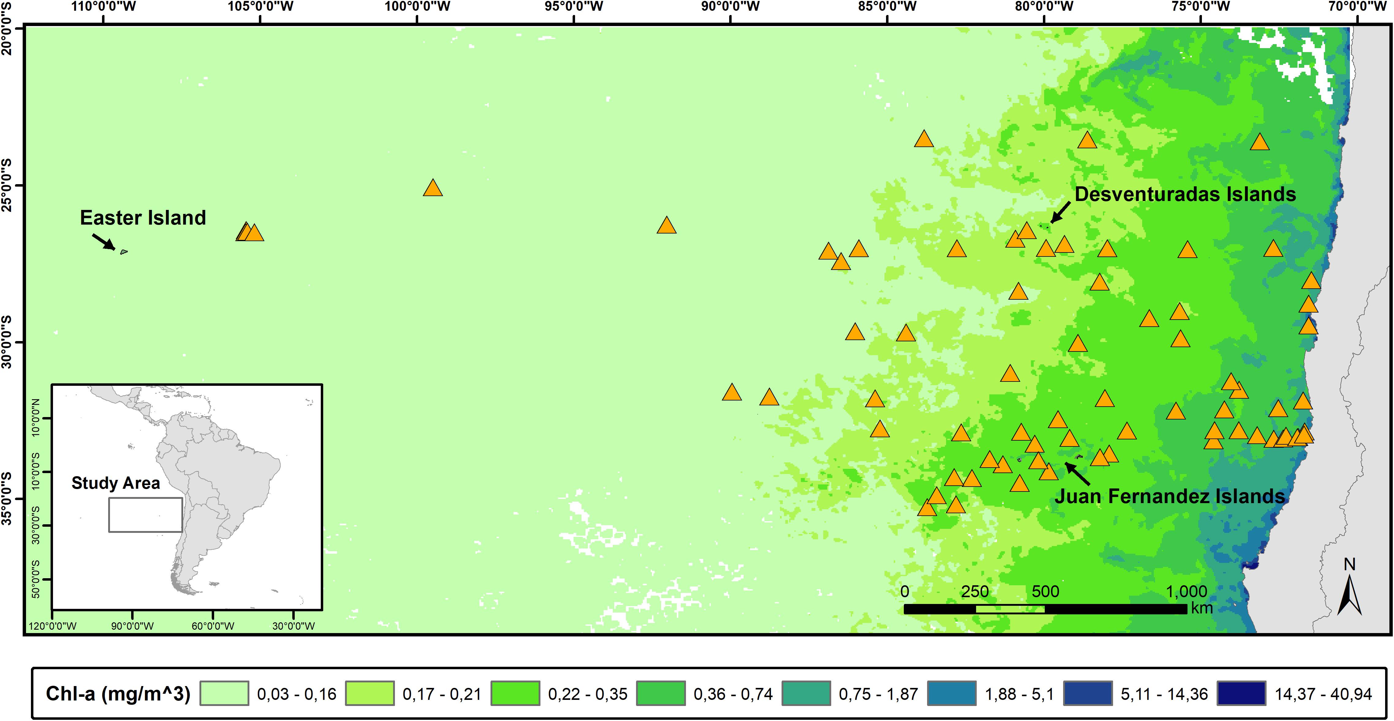
Figure 1. Map of the South-East Pacific Ocean showing the position of the daily surveys (orange triangles) and main island systems. To illustrate the gradient in primary productivity in the area (represented by chlorophyll α concentration), we overlaid a satellite image from the Aqua MODIS –Terra satellite corresponding to September 2014.

Our study aims to quantify the geographical patterns of seabird abundance, species richness, and assemblage distribution in the ESPO, and to assess how environmental conditions influence these patterns. We hypothesize that seabird assemblages are spatially structured by the underlying patterns in the oceanic environment. To test our hypothesis, we employ a spatially explicit approach by applying multivariate techniques to investigate the biogeographic structure of seabird assemblages, in relation to oceanographic properties.

Materials and Methods

Study Area

Our study area, spanning ∼3500 km from the west coast of South America to Rapa Nui (Easter Island), is characterized by strong gradients in water mass properties and primary productivity, which can vary by three orders of magnitude (Figure 1). The eastern limit of our study area is bounded by the Humboldt Current, which is characterized by a northward flow of surface waters of sub-Antarctic origin and by upwelling of deeper, nutrient-rich waters from the equator. The upwelling of nutrients along the west coast of South America results in extremely high primary productivity that fuels higher trophic levels (e.g., zooplankton, fish, seabirds, marine mammals) (Thiel et al., 2007). In contrast, at the opposite end lays the South Pacific Gyre; an extensive oceanic area marked by very low primary productivity, and subtropical surface waters of high temperature and salinity (Longhurst, 2007; Morel et al., 2010). At the center of our study area lay two important archipelagos: Juan Fernández and Desventuradas Islands, both of which influence the regional oceanography. Particularly, the presence of these two archipelagos increases local primary productivity through the “island mass effect,” influencing the ecology of the surrounding regions (Andrade et al., 2012, 2014). The area hosts an important marine biodiversity which has been internationally recognized by the creation of several marine protected areas: four no-catch Marine Parks (level IA IUCN) (Nazca-Desventuradas, Mar de Juan Fernández, Montes Submarinos Crusoe y Selkirk, and Motu Motiro Hiva) and two Marine and Coastal Protected Areas, which allows limited human activities (level IV UICN) (Mar de Juan Fernández and Rapa Nui).

Seabird Surveys

To estimate seabird abundance and richness at-sea, we conducted surveys on board vessels traveling across the study area, from the coast of continental Chile to Rapa Nui (Easter Island). We participated in 11 cruises spanning from September 2014 to September 2017 (Supplementary Table S1). Seabird counts were conducted using 10-min bins, following standardized strip transect methods (Tasker et al., 1984; van Franeker, 1994). Surveys were conducted from sunrise to sunset with short breaks every 3–4 h to mitigate observer fatigue (Spear et al., 2004). Located in the flying bridge, a trained observer identified to the lowest taxonomic level all birds sighted within 300 m off the vessel in a 90° arc from the bow to the beam. Observers also noted behavior (e.g., flying, sitting, ship following), relative age (juvenile or adult), and weather conditions (Beaufort Sea State). Ship-following birds were recorded when first sighted and ignored thereafter. On some cruises, two observers independently surveyed both sides of the vessel, doubling the width of the strip transect to 600 m. The vessel route was recorded using a handheld GPS (Garmin GPSmap 62s).

Data Processing: Seabird Sightings

Prior to statistical analysis we addressed three limitations of the seabird sighting data. First, we included only those species that breed in the South-East Pacific, if any of their breeding colonies occurred between 0° and 60° S latitude and 67° and 130° W longitude. We only included those species that breed on islands located within the study area, because we expected that, during reproduction, the distributions of these central-place foragers would be constrained to the environmental conditions around their colonies. Conversely, we expected that the at-sea distributions of non-breeding species, migrating seasonally through the study area, would not be spatially structured in response to the oceanic environment. Next, to deal with those birds that could not be identified to species level, we developed nine taxonomic groupings: ALBSP = Thalassarche sp., ARDSP = Ardenna sp., FARBSP = Cookilaria group, GOLMSP = Storm-petrels, GPSP = Macronectes sp., PTESP = Pterodroma sp., PUFSP = Puffinus sp., STERSP = Skuas, and STSP = Terns. Finally, because of the small number of individuals recorded from two species that are inherently difficult to identify at sea, we pooled their counts with these broader taxonomic groupings; the Chilean skua (Catharacta chilensis) was included in the STERSP, and the Southern Giant Petrel (Macronectes giganteus) was included in the GPSP. The processed dataset involved 35 regionally breeding taxa: 26 species, and 9 multi-species taxonomic groupings (Supplementary Table S2).

Data Processing: Survey Effort

Because we relied on platforms of opportunity vessels, involving three cruises onboard scientific vessels and eight cruises chartered by the Chilean Navy, the surveys were highly heterogeneous, and varied in the total duration, the daily itinerary, and the areal extent and coverage. Namely, while some cruises entailed uninterrupted transit at a fairly constant speed and direction (7 out of 11), other cruises entailed repeatedly zig-zagging around seamounts and islands.

To avoid potential biases resulting from this sampling heterogeneity, we processed the data and selected the surveys based on five criteria. First, all 10-min bins from the same day were pooled, making a single daily transect the sample unit for further analyses. Second, because the strip transect methodology requires the vessel to maintain a constant speed and direction (Tasker et al., 1984; van Franeker, 1994), we only considered those transects that fulfilled this requirement. Third, we removed the inherent influence of abundance on species richness, which can obscure the mechanism driving beta-diversity variability when analyzing patterns of uneven site-assemblage composition (i.e., beta-diversity; Lennon et al., 2001; Baselga et al., 2007; Kreft and Jetz, 2010). To this end, we correlated the species richness (log transformed) and the seabird abundance (log transformed) in each daily survey and progressively eliminated those samples with the lowest bird abundances, until no highly significant relationship (P > 0.001) between these variables existed. Following this iterative approach, the highly significant correlation (r = 0.75, P < 0.001) and shared variability (r² = 56%) between these variables were reduced substantially (r = 0.27, P = 0.018, r² = 7%) when only surveys with abundance >15 birds were included in the analysis. By discarding those surveys where low seabird abundances constrained species richness, we improved our ability to explore the pattern of variability in the site-assemblage composition. Fourth, in the same line as previous, we discarded the species that were not present in at least 3% of the surveys. Finally, we explored the influence of the variable amount of area surveyed per daily transect on the number of seabirds encountered. Thus, because a generalized linear model (GLM) with a Poisson probability revealed that these variables were not related (pseudo r² = 0.3%), we considered all daily transects regardless of the area surveyed. Consequently, all further calculations were based on seabird densities (birds km^–2) calculated during 72 daily transects.

Environmental Factors

We used 10 environmental variables to describe and characterize the oceanographic habitats of the seabird assemblages: seven were dynamic and three were static (Table 1). The Aqua MODIS (Moderate Resolution Imaging Spectroradiometer) satellite, from NASA (National Aeronautics and Space Administration), yielded mean sea surface temperature (SST) (°C) and mean sea surface chlorophyll α (mg m^–3). Even though chlorophyll α quantifies the standing stock of phytoplankton, it is routinely used as a proxy for primary productivity, and to model marine species distributions (Tremblay et al., 2009). To quantify spatial gradients in SST and chlorophyll α, we calculated the relative magnitude of change using the coefficient of variation (CV = 100% ^∗ standard deviation/mean) of these two variables during each sampling day (Hyrenbach et al., 2006). This allowed us to determine if we had crossed any major hydrographic features (e.g., fronts, mesoscale eddies), which are known to influence seabird distribution (Bost et al., 2009; Force et al., 2015). As a result, two new derived variables were included: CV of the SST (%) and CV of the sea surface chlorophyll α (%). We also included two publicly available variables from the CMEMS (Copernicus Marine Environment Monitoring Service) website¹ : mean sea surface salinity (SSS) (ppt), and mean mixed layer depth (m) (Guinehut et al., 2012). Additionally, because wind is an important factor affecting seabird distribution at global (Davies et al., 2010) and regional scales (Weimerskirch et al., 2012), mean wind speed (m s^–1) data from the ASCAT (Advanced Scatterometer) sensor in the Metop satellite were obtained from the CERSAT-Ifremer website².

TABLE 1

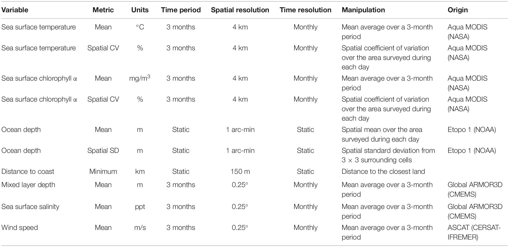
Table 1. Environmental variables employed in the analysis.

All dynamic variables were sampled or calculated with a temporal resolution of 1 month, and averaged over a 3-month period to develop a seasonal composite. Because our study focuses on the influence of long-lasting oceanographic conditions (e.g., water masses, fronts) on seabird community composition, this composite integrated short-term variability (i.e., eddies, meanders) and captured seasonal and inter-annual environmental variability (Mannocci et al., 2014).

Three static environmental variables were also considered as potential drivers of seabird assemblage distributions (Table 1): ocean depth, spatial standard deviation of ocean depth, and distance to the coast. We derived ocean depth (m) from the National Geophysical Data Center NOAA ETOPO1 Global Relief Model (Amante and Eakins, 2009). To account for spatial changes in bathymetry (e.g., seamounts, shelves), we calculated the spatial standard deviation for each grid, cell using the 3 ^∗ 3 surrounding grid cells to develop the spatial standard deviation of ocean depth. We also included distance to the nearest coast (km), which is a proxy for distance to colonies that can influence the foraging distributions of breeding seabirds (Veit, 1995; Hyrenbach et al., 2006; Renner et al., 2013; Santora et al., 2017). Colonies are located in the main islands (Easter Island, Juan Fernández, and Desventuradas), and widespread throughout the mainland coast.

Finally, we included Julian day to account for the influence of seabird phenology in our sampling (Ainley et al., 2005). The timing of the surveys likely will influence community composition, as some breeding species [e.g., Juan Fernández Petrel (Pterodroma externa) and Pink-footed Shearwater (Ardenna creatopus)] are present in the area during the summer breeding period, and disperse across the Pacific Ocean thereafter (Ainley and Boekelheide, 1983).

Prior to further analysis, the collinearity of all explanatory variables was checked using the variance inflation factor (VIF). All VIF values were <10 (Supplementary Table S3), indicating low collinearity between variables (O’Brien, 2007). While SST and SSS were cross-correlated (r = 0.7), we retained both variables for the analysis, because frontal systems and water mass boundaries are often associated with temperature and color fronts (e.g., Pichel et al., 2007), and they are indicative of different physical and biological processes known to influence seabird distributions (Hyrenbach et al., 2006, 2007).

Statistical Analysis

To investigate the relationship between environmental explanatory variables and assemblage composition we used multivariate generalized models (GLMs). The models were constructed using the manyglm function available in the package mvabund (Wang et al., 2012), and fitting a negative binomial distribution appropriate for count data. Model selection was performed using the drop1 function from the package stats based on the Akaike Information criterion to select the most parsimonious model (Crawley, 2007). After that, model significance was calculated using a likelihood ratio test and p-values were assigned following 999 pit-trap resampling iterations using the anova.manyglm function. To visualize differences in assemblage composition we constructed non-metric multi-dimensional scaling (NMDS) plots using the metaMDS function from the vegan package (Oksanen et al., 2013). To construct the NMDS, we first produced a distance matrix based on the Bray–Curtis metric. One of the preliminary requirements to perform an NMDS is to choose an a priori number of axes before performing the ordination. After running several tests, we concluded that three dimensions, with an associated stress of 0.15, provided the best compromise for obtaining the most complete ordination, without overfitting the model. Stress values < 0.20 indicate good model performance (Clarke, 1993).

To further characterize the seabird assemblage distributions, we performed a clustering analysis to identify discrete groups of samples (daily surveys) using the cluster package (Maechler et al., 2019). We first constructed a relative Euclidean distance matrix, which was then used to build an unweighted pair group method with arithmetic mean (UPGMA) hierarchical agglomerative clustering analysis (Legendre and Legendre, 1998). The groups resulting from the clustering were plotted in the NMDS ordination space to assess the congruence between both methods (Kreft and Jetz, 2010).

Finally, we explored the influence of the environmental factors on seabird species richness and overall abundance (abundances of all species pooled together) by fitting GLMs. Specifically, to analyze the richness–environment relationships we used GLM with a Poisson distribution and log-link function, whereas for the abundance (birds km^–2)–environment relationships, we employed GLM with a Gamma distribution and inverse-link function. Model selection (Burnham and Anderson, 2002) and averaging were performed using the R package MuMIn (Barton, 2018).

All analyses were performed using the statistical software R (R Core Team, 2016).

Results

Seabird Surveys

After discarding survey bins to account for the heterogeneity in survey effort across cruises, our dataset involved a total of 72 daily transects, spanning ∼3547 km² of ocean surveyed and ∼9121 km traveled (Supplementary Table S1). The total number of seabirds recorded encompassed 6697 individuals belonging to 26 different species and 9 taxonomic groupings. The three most common species were Juan Fernández Petrel (30.63%), Masatierra Petrel (Pterodroma defilippiana) (9.82%), and Sooty Shearwater (Ardenna grisea) (7.18%) (Supplementary Table S2).

Seabird Assemblages

The cluster analysis identified four groups of daily transects with different species composition and distinct spatial distributions across the study area (Figure 2A). Mapping these groups in geographic space revealed two spatial patterns. Two of the groups showed a clear segregation, only occurring closer to the Humboldt Current (farther east) or closer to Easter Island (farther west), indicative of a longitudinal structuring of the seabird assemblages. The other two groups, which correspond to sites located around the Juan Fernández and Desventuradas archipelagos, showed a less obvious spatial segregation (Figure 2B).

FIGURE 2

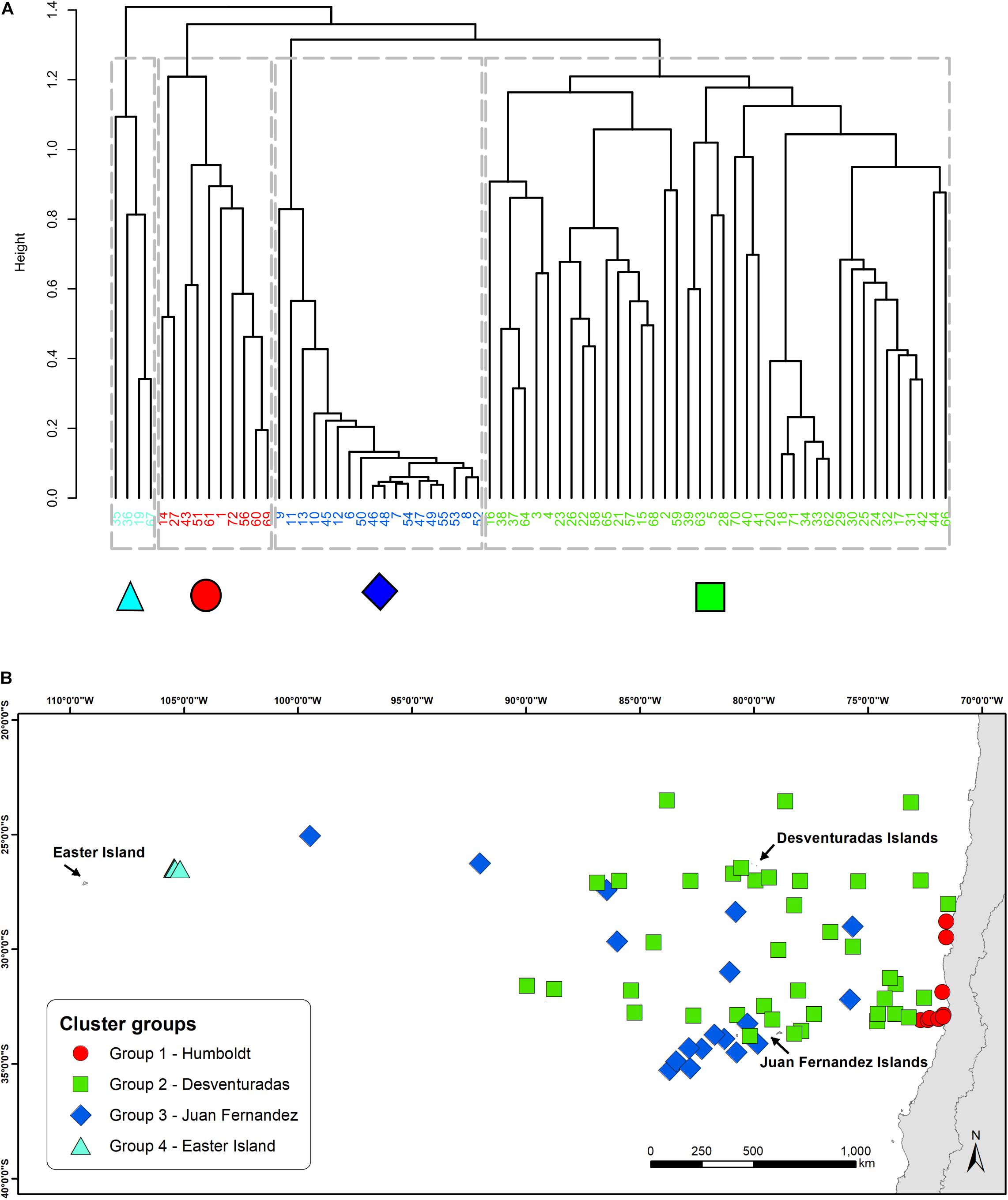
Figure 2. Cluster analysis (A) dendrogram representing the results from the UPGMA agglomerative hierarchical clustering. Dashed lines show the level of similarity chosen to obtain four clusters. Colors and symbols of each site correspond to the group they belong to. (B) Geographical distribution of the sampled sites and their belonging to the different cluster groups. Each symbol and color correspond to one group. Each group is named after the closest oceanographic system.

The results from the NMDS ordination reinforced those from the clustering, positioning the daily transects from Humboldt and from Easter Island on the opposite extremes of axis 1 (Figure 3). The rest of the transects laid between these two extremes, showing substantial overlap along axis 1. However, axis 2 allowed us to discriminate between the other two clusters of daily transects, underscoring differences between the assemblages surrounding the Desventuradas and Juan Fernández archipelagos.

FIGURE 3

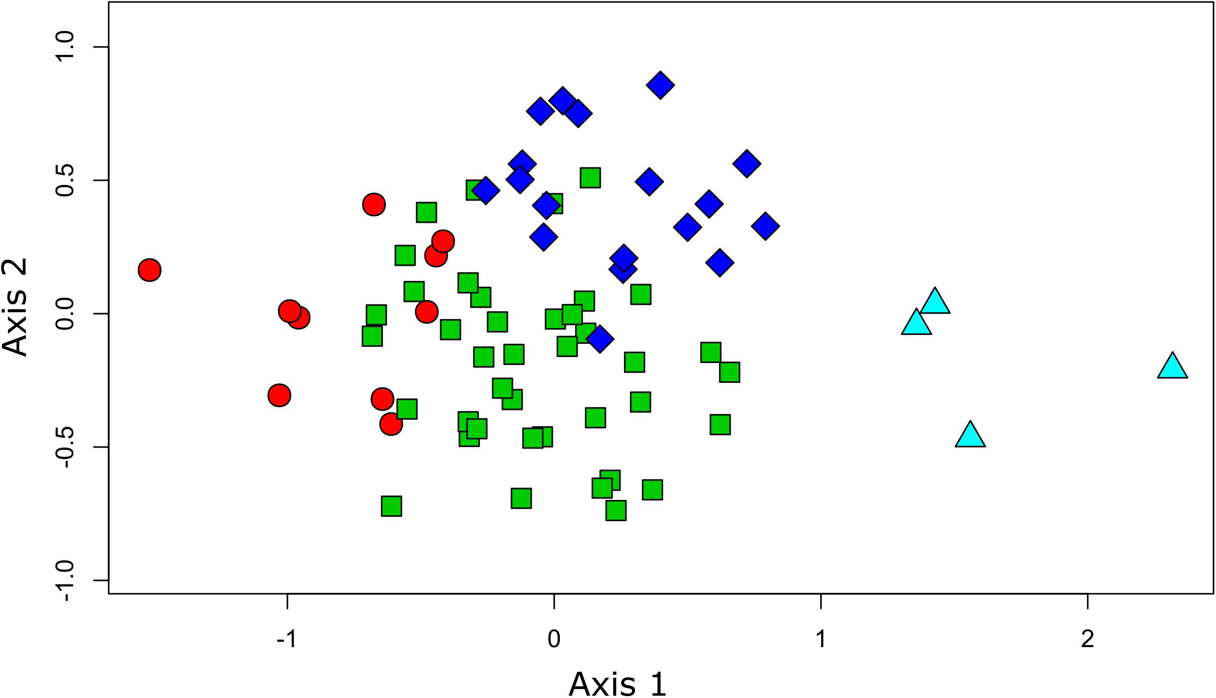
Figure 3. Plot of sampled sites showing the results from the NMDS ordination (1st and 2nd axis) overlaid on the results from the clustering analysis. The different colors and shapes of the sites correspond to the different groups found (Figure 2) (circles: Humboldt, triangles: Easter I, squares: Juan Fernández, and diamonds: Desventuradas).

The multivariate GLM highlighted the importance of five different environmental variables: Julian day, ocean depth, sea surface chlorophyll α, SST (mean), and SSS (mean). From these, surface chlorophyll α showed the highest explanatory power, while SST (mean) showed the lowest (Table 2).

TABLE 2

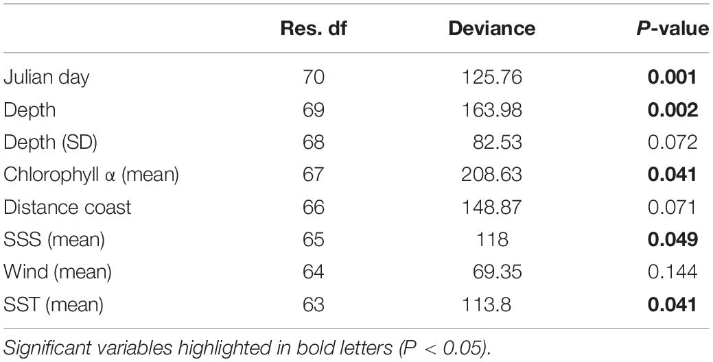
Table 2. ANOVA table from the most parsimonious multivariate generalized linear model showing variance explained by each variable (deviance) and the significance after 999 PIT-trap resampling iterations (P-value).

The GLMs testing the environment–species richness relationship showed that Julian day and SST (CV) were the most important variables. A total of 10 models were selected as the best-fitting models; Julian day appeared in all of these models, while SST (CV) appeared in eight of them, showing the best performance of all environmental variables (Table 3A). The environment–abundance GLM models showed a less clear tendency in relation to variable importance. Distance to the coast and ocean depth (SD) was present in all of the 12 models selected, while mixed layer depth (mean) and SSS (mean) were present in 11 (Table 3B). Altogether, these results highlight the influence of dynamic [SST (CV), mixed layer depth, SSS] and static (depth, distance to the coast) environmental factors and of seasonality (Julian day) on the overall abundance and species richness of seabirds. In addition to the influence of these multiple environmental factors, our surveys identified four robust biogeographic assemblages, associated with specific oceanographic domains (current systems) and archipelagos (nesting grounds).

TABLE 3

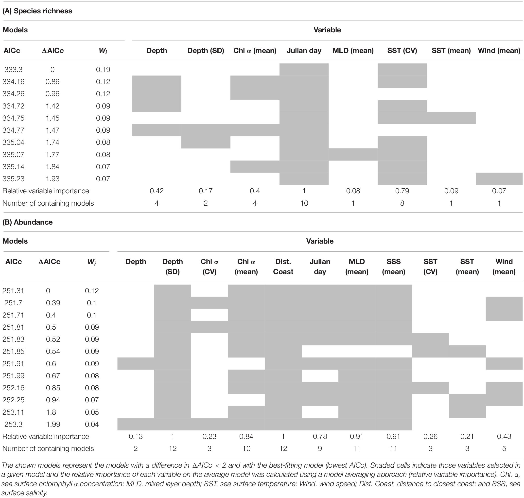
Table 3. Best-fitting GLMs showing the most important environmental variables in the relationships environment-species richness (A) and environment-abundance (B).

Discussion

Our analyses revealed a clear spatial pattern of seabird species composition across the ESPO, with four distinct assemblages spreading from the Humboldt Current (east) to Easter Island (west), and with evidence of some latitudinal separation, associated with the presence of the Desventuradas (north) and Juan Fernández (south) archipelagos (see Supplementary Table S4 for a list of species breeding in the different islands). Three inter-related environmental variables had an important influence on the distribution of these assemblages: SSS, SST, and sea surface chlorophyll α. These dynamic oceanographic characteristics captured a major longitudinal gradient spanning the study area: cold, nutrient-rich, and low salinity waters in the east (Humboldt Current) and warm, nutrient-poor, and high salinity waters in the west (South Pacific Gyre). Moreover, this co-variability was evident in the VIF analysis, which identified cross-correlations among these three variables. Two more variables showed a high importance in the models regarding assemblage composition: Julian day and depth. Julian day captures the seasonality of seabird distributions, which is obvious for species that breed in the study area during the boreal summer (November–April) and disperse across the Pacific Ocean thereafter. Thus, the species-specific breeding and migration cycles influence the overall composition and species richness (see below) of the seabird assemblage in the study area. The influence of depth may be related to onshore–offshore gradients in seabird distributions, as has been previously documented in the broad continental shelves in the Bering Sea (Hunt et al., 2014; Santora et al., 2017) and the South Atlantic (Veit, 1995). While the Chilean continental shelve is relatively narrow, abrupt bathymetric changes (e.g., shelf-breaks and slopes) also structure seabird assemblages, likely due to changes in water flow and prey distributions (Schneider, 1997). In particular, coastal species from the Humboldt Current assemblage may be linked to the shallow waters of the continental shelf, unlike the far-ranging oceanic species.

Previous works have described SST and SSS as important environmental variables influencing seabird assemblages (Hyrenbach et al., 2007; Commins et al., 2014; Force et al., 2015). Moreover, these variables are regularly used to describe water masses, with seabird species distributions often mirroring their changes at macro-scales (Pocklington, 1979; Wahl et al., 1989). However, there is little understanding about the mechanisms underlying these seabird–water mass relationships, because seabirds are not directly consuming the nutrients tightly associated with these physical tracers. Yet, SST and SSS are indicators of oceanographic processes and features that influence the abundance and composition of marine biota, both planktonic and nektonic (Longhurst, 2007). Thus, seabird assemblages likely reflect the distribution of their lower trophic level prey (Ashmole, 1971; Pocklington, 1979). For instance, several characteristic seabird species from the Humboldt Current [e.g., Humboldt Penguin (Spheniscus humboldti), Peruvian Booby (Sula variegata)] forage on schooling fish (e.g., Engraulis ringens, Strangomera bentincki) (Jahncke and Goya, 1998; Herling et al., 2005). Because the distribution of these schooling fishes in the ESPO is restricted to the Humboldt Current, those seabird species highly dependent on this resource would be similarly constrained, thus geographically delineating a distinct seabird assemblage. On the other hand, tropical and subtropical seabirds [e.g., Masked Booby (Sula dactylatra), Red-tailed Tropicbird (Phaethon rubricauda)] are highly dependent on flying fishes (Exocoetidae) and squids (Ommastrephidae) (Carboneras et al., 2019; Orta et al., 2019) that inhabit warm surface waters and are not present in the colder, nutrient-rich waters of the Humboldt Current. Therefore, the distribution of tropical and subtropical seabirds in the ESPO could be driven by the availability of these epipelagic prey and the subsurface predators (predatory fishes and tunas) that drive them to the surface and into the air (Ballance and Pitman, 1999; Spear et al., 2007). To date, different authors have proposed that patterns of prey distribution may drive the biogeographic structure of seabirds over macro and mega-scales (Ainley and Boekelheide, 1983; Abrams, 1985; Sydeman et al., 2010; Sigler et al., 2017). While our findings point in that direction, further research is needed to fully understand how these predator–prey relationships influence species distributions. Many factors can mediate between the abundance and availability of prey, including the degree of prey aggregation, their vertical distribution, and their habitat associations (Benoit-Bird et al., 2011, 2013; Suryan et al., 2016). In particular, our results underscore the importance of productivity (chlorophyll α concentration) as a driver of seabird assemblages. Previous studies documented this same influence in the Pacific and Indian oceans (Pocklington, 1979; Ballance et al., 1997; Ribic et al., 1997). Altogether, these results highlight the need to understand how the structure of marine food webs influences the identity and the abundance of the various seabird prey, especially when many oceanic seabirds have broad diets (Ballance and Pitman, 1999; Spear et al., 2007).

In the same way the spatial pattern in seabird assemblages was related to environmental factors, species richness was also influenced by these factors. Particularly, our study shows that species richness was highly related to Julian day and SST (CV). We used SST (CV) as a proxy for the presence of water mass boundaries and fronts. These areas have been described as important features in the distribution of seabirds via two mechanisms. They can act as areas of primary productivity enhancement and prey concentration, which often leads to higher seabird abundance (Bost et al., 2009; Scales et al., 2014), and they can act as biogeographic boundaries, separating different seabird assemblages (Commins et al., 2014; Force et al., 2015). Daily transects crossing these boundaries would be expected to capture species present in both water masses and along the front, thus yielding high species richness. In particular, areas of higher SST (CV) likely correspond to the western limit of the Humboldt Current, where sharp changes in oceanographic conditions occur (Thiel et al., 2007). Interestingly, because the daily transects belonging to the Humboldt Current group are located close to shore, the area influenced by this current system seems to be very restricted to the coast (≈100 km).

The influence of Julian day on species richness reflects the strong seasonality in the distribution of several species that breed in the area [e.g., Juan Fernández Petrel, Stejneger’s Petrel (Pterodroma longirostris), pink-footed shearwater]. For instance, the Juan Fernández Petrel breeding population during the austral summer, which has been estimated at 1,000,000 pairs (BirdLife International, 2018), migrates to northern latitudes and spends the rest of the year in the North Pacific. Thus, the presence of these breeding species in the study area is highly dependent on the time of the year, which in turn influences the overall species richness in the study area, especially in the vicinity of their breeding islands.

The abundance of seabirds in the study area is related to several environmental factors indicative of a mixture of oceanographic processes. Distance to the colonies and depth (SD) are indicative of onshore–offshore gradients in seabird abundance, as has been suggested as an explanation for the at-sea distribution of seabirds (Ballance et al., 1997; Hyrenbach et al., 2006; Mannocci et al., 2014). The spatial restriction imposed on seabirds during the breeding season has been postulated as one reason behind this relationship, resulting in increased abundances near colonies. Usually, distance to the coast of the breeding colonies (i.e., islands or mainland) is linked to the depth. However, changes in seafloor topography because of ridges or seamounts play an essential role in aggregating top predators, such as tunas and seabirds (Morato et al., 2008, 2010). Two important bathymetric features are present in our study area: the Nazca Ridge and the Easter Seamount Chain (Ray et al., 2012). The importance of depth (SD) in our models could be related to these topographic features in addition to onshore–offshore gradients away from breeding colonies. Further surveys are necessary to clarify the extent of seabird halos around these breeding colonies, and the influence of ridges and seamounts on seabird distribution in the ESPO. The other two variables also important in explaining changes in seabird abundance (mixed layer depth and SSS) are related to the influence of coastal upwelling (Ainley et al., 2005). The thickness of the mixed layer depth is greatly influenced by upwelling of nutrient-rich and cold waters into the mixed layer, affecting localized primary productivity and seabird prey availability (Ballance et al., 1997). In our study area, both variables follow a longitudinal gradient increasing toward the west, as they move away from the Humboldt Current. This gradient is also reflected in the habitat characteristics of the four seabird species clusters, which correspond to four distinct biogeographic domains (Table 4).

TABLE 4

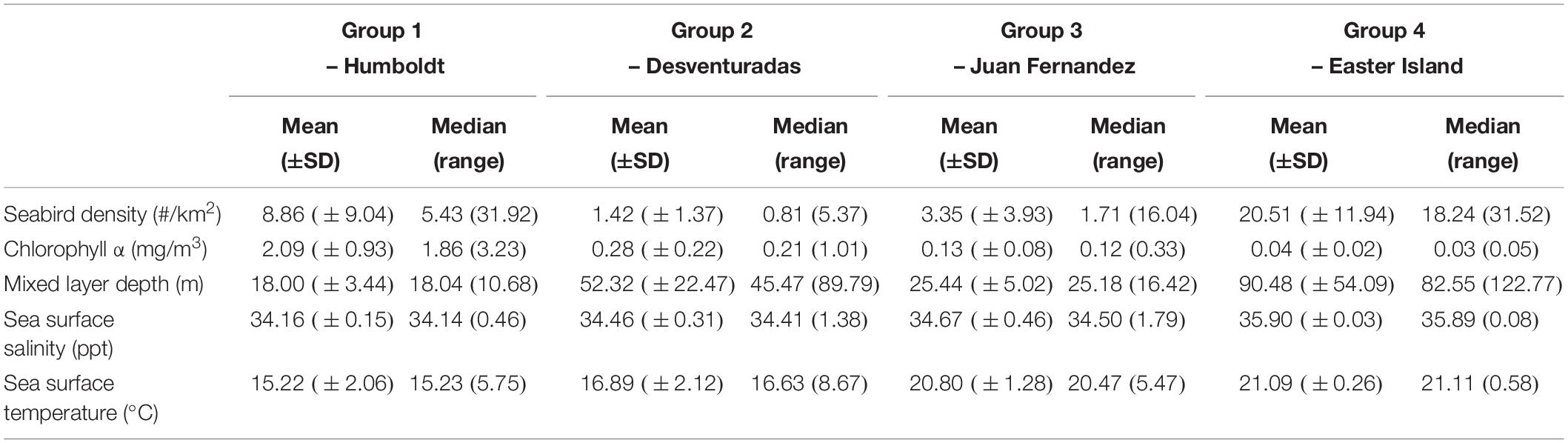
Table 4. Oceanographic and biological characteristics of the biogeographic domains associated to the four cluster groups, defined by ocean productivity (seabird density of all species combined, chlorophyll α concentration, mixed layer depth), and surface water masses (temperature, salinity).

The geographical distribution of these four groups, identified by the cluster analysis, revealed a longitudinal and latitudinal spatial pattern of seabird assemblages. Previous biogeographical studies from the area, focusing on coastal ecosystems, have identified similar patterns, assigning four different ecoregions in the area: Humboldt, Easter Island, Juan Fernández, and Desventuradas (Rovira and Herreros, 2016). At both extremes of this longitudinal spatial structure, we could identify two well-defined, spatially divided groups (Humboldt and Easter Island). The NMDS analysis supports this pattern by placing these groups in the opposite extremes of the ordination (related to axis 1). The species composition of these two groups shows virtually no overlap, since no species are shared between them (Supplementary Table S2). However, the other two groups do not show such a clear spatial differentiation, with a more diffuse (Desventuradas) and aggregated (Juan Fernández) geographical distribution around the two archipelagos. In the NMDS ordination space both groups are not differentiated in axis 1, but show a segregation in relation to axis 2, meaning that species composition does differ between both groups. The assemblages identified for both groups using at-sea distributions reflect those assemblages of nesting seabirds in Juan Fernández and Desventuradas, respectively (Figure 2). Both archipelagos are different at the level of their islands’ physiography; the three islands of Desventuradas are relatively small, in the range of 0.25–2.2 km², with maximum heights of 166–479 m, while the three islands of Juan Fernández are in the range of 5–93 km², and maximum heights of 375–1650 m. Despite their proximity, it seems that differences in the physiographic and climatic factors (Bahamonde, 1987; Hajek and Espinoza, 1987) affect the existence of different vegetation in these archipelagos (Hoffmann and Marticorena, 1987), which in turn provides nesting habitat for substantially different breeding seabird assemblages (see Supplementary Table S4). However, at-sea distributional differences become diluted away from the breeding islands, with no clear spatial segregation. This result has important management implications, since conservation actions in the surrounding waters of one archipelago could have implications for seabird communities in both archipelagos.

This study shows that seabird assemblages in ESPO are spatially structured through a large-scale longitudinal gradient that extends from the Humboldt Current System to Rapa Nui. The observed pattern is related to Julian day, ocean depth, and surface levels of chlorophyll, temperature, and salinity. How seabirds respond to environmental factors and how they partition the ocean habitat is crucial to understand their ecology, life-history traits, and conservation threats (Croxall et al., 2012; Lewison et al., 2012). Knowledge of the distribution patterns and assemblage composition during the time they are at sea would be beneficial for declaring and delimiting marine protected areas in the ocean. For example, four large marine protected areas (Nazca-Desventuradas, Mar de Juan Fernández, Crusoe and Selkirk Submarine Mountains, and Motu Motiva Hiva) were recently established in the ESPO, based on criteria related to the existence of a great diversity of invertebrates and fish, some with a high degree of endemism (e.g., Friedlander et al., 2013). However, seabirds were only partially considered in these spatial conservation actions, although they play an essential role supporting the other components of marine biodiversity (e.g., Graham et al., 2018). The results of this study will be useful for decision-makers and political authorities to assess the degree of compliance with the conservation objectives established in the decree creating marine protected areas and recommend actions that allow the integral protection of the biodiversity they contain.

Data Availability Statement

The datasets generated for this study are available on request to the corresponding author.

Author Contributions

GL-J and JS designed and conceived the study. JS, MP-T, NL, and DM-U collected the data. JS and KH analyzed the data and wrote first versions of the manuscript. JS, KH, and GL-J corrected and wrote the final version of the manuscript. All authors reviewed and contributed to the writing of the final version of the manuscript.

Funding

This study was funded by the Chilean Millennium Initiative ESMOI. JS was supported by the Comisión Nacional de Ciencia y Tecnología (CONICYT), Programa Beca Doctorado Nacional, Chile (Grant No. 21150640). KH was supported by an HPU paid research leave (PRL) award.

Conflict of Interest

The authors declare that the research was conducted in the absence of any commercial or financial relationships that could be construed as a potential conflict of interest.

Acknowledgments

We want to thank the Armada de Chile for their help and support during data collection on the board of their cruises. Also, we would like to thank the Comité Oceanográfico Nacional (CONA) from Chile, for funding the cruises CIMAR 21-15-113 and CIMAR 22-16-06 to GL-J. We acknowledge the comments and suggestions of MA and KK, who contributed to improve our study substantially.

Supplementary Material

The Supplementary Material for this article can be found online at: https://www.frontiersin.org/articles/10.3389/fmars.2019.00838/full#supplementary-material

Footnotes

1. ^ http://marine.copernicus.eu/
2. ^ http://cersat.ifremer.fr/

References

Abrams, R. W. (1985). Environmental determinants of pelagic seabird distribution in the African sector of the Southern Ocean. J. Biogeogr. 12, 473–492. doi: 10.2307/2844955

CrossRef Full Text | Google Scholar

Ainley, D. G., and Boekelheide, R. J. (1983). An ecological comparison of oceanic seabird communities of the south Pacific Ocean. Stud. Avian Biol. 8, 2–23.

Google Scholar

Ainley, D. G., Ribic, C. A., and Spear, L. B. (1993). Species-habitat relationships among seabirds: a function of physical or biological factors? Condor 95, 806–816. doi: 10.2307/1369419

CrossRef Full Text | Google Scholar

Ainley, D. G., Ribic, C. A., and Woehler, E. J. (2012). Adding the ocean to the study of seabirds : a brief history of at-sea seabird research. Mar. Ecol. Prog. Ser. 451, 231–243. doi: 10.3354/meps09524

CrossRef Full Text | Google Scholar

Ainley, D. G., Spear, L. B., Tynan, C. T., Barth, J. A., Pierce, S. D., Ford, R. G., et al. (2005). Physical and biological variables affecting seabird distributions during the upwelling season of the northern California current. Deep Sea Res. Part II Top. Stud. Oceanogr. 52, 123–143. doi: 10.1016/j.dsr2.2004.08.016

CrossRef Full Text | Google Scholar

Amante, C., and Eakins, B. W. (2009). ETOPO1 1 Arc-Minute Global Relief Model: Procedures, Data Sources and Analysis. NOAA Technical Memorandum NESDIS NGDC-24. Boulder, CO: National Geophysical Data Center, 19. doi: 10.1594/PANGAEA.769615

CrossRef Full Text | Google Scholar

Andrade, I., Hormazabal, S. E., and Correa-Ramirez, M. A. (2012). Annual cycle of the satellite chlorophyll-a in the Juan Fernández archipelago (33°S), Chile. Lat. Am. J. Aquat. Res. 40, 657–667. doi: 10.3856/vol40-issue3-fulltext-14

CrossRef Full Text | Google Scholar

Andrade, I., Sangrà, P., Hormazabal, S., and Correa-Ramirez, M. (2014). Island mass effect in the Juan Fernández Archipelago (33°S), Southeastern Pacific. Deep Sea Res. Part I Oceanogr. Res. Pap. 84, 86–99. doi: 10.1016/j.dsr.2013.10.009

CrossRef Full Text | Google Scholar

Ashmole, N. P. (1971). “Sea bird ecology and the marine environment,” in Avian Biology, Vol. 1, eds D. S. Farner, J. R. King, and K. C. Parkes, (New York, NY: Academic Press), 223–286.

Google Scholar

Bahamonde, N. (1987). “San Félix and San Ambrosio the Desventuradas Islands,” in Islas Oceánicas Chilenas: Conocimiento Científico y Necesidades de Investigación, ed. J. C. Castilla, (Santiago: Ediciones Universidad Católica de Chile), 85–100.

Google Scholar

Ballance, L. T., and Pitman, R. L. (1999). “Foraging ecology of tropical seabirds,” in Proceedings of the 22nd International Ornithological Congress, eds N. J. Adams, and R. H. Slotow, (Johannesburg: Bird Life South Africa), 2057–2071.

Google Scholar

Ballance, L. T., Pitman, R. L., and Reilly, S. B. (1997). Seabird community structure along a productivity gradient: importance of competition and energetic constraint. Ecology 78, 1502–1518. doi: 10.1890/0012-9658(1997)078[1502:SCSAAP]2.0.CO;2

CrossRef Full Text | Google Scholar

Barton, K. (2018). MuMIn: Multi-Model Inference. R Package Version 1.15.1. Available at: https://cran.r-project.org/web/packages/MuMIn/index.html (accessed August 20, 2019).

Google Scholar

Baselga, A., Jiménez-Valverde, A., and Niccolini, G. (2007). A multiple-site similarity measure independent of richness. Biol. Lett. 3, 642–645. doi: 10.1098/rsbl.2007.0449

PubMed Abstract | CrossRef Full Text | Google Scholar

Benoit-Bird, K. J., Battaile, B. C., Heppell, S. A., Hoover, B., Irons, D., Jones, N., et al. (2013). Prey patch patterns predict habitat use by top marine predators with diverse foraging strategies. PLoS One 8:e53348. doi: 10.1371/journal.pone.0053348

PubMed Abstract | CrossRef Full Text | Google Scholar

Benoit-Bird, K. J., Kuletz, K., Heppell, S., Jones, N., and Hoover, B. (2011). Active acoustic examination of the diving behavior of murres foraging on patchy prey. Mar. Ecol. Prog. Ser. 443, 217–235. doi: 10.3354/meps09408

CrossRef Full Text | Google Scholar

BirdLife International, (2018). Pterodroma externa. The IUCN Red List of Threatened Species 2018: e.T22698030A132620783. Available at: http://dx.doi.org/10.2305/IUCN.UK.2018-2.RLTS.T22698030A132620783.en (accessed March 11, 2019).

Google Scholar

Bost, C. A., Cotté, C., Bailleul, F., Cherel, Y., Charrassin, J. B., Guinet, C., et al. (2009). The importance of oceanographic fronts to marine birds and mammals of the southern oceans. J. Mar. Syst. 78, 363–376. doi: 10.1016/j.jmarsys.2008.11.022

CrossRef Full Text | Google Scholar

Brown, R. G. B., Cooke, F., Kinnear, P. K., and Mills, E. L. (1975). Summer seabird distributions in Drake Passage, the Chilean fjords and off southern South America. Ibis 117, 339–356. doi: 10.1111/j.1474-919X.1975.tb04221.x

CrossRef Full Text | Google Scholar

Burnham, K. P., and Anderson, D. R. (2002). Model Selection and Multimodel Inference: A Practical Information-Theoretic Approach, 2nd Edn. New York, NY: Springer. doi: 10.1002/1521-3773(20010316)40:6<9823::AID-ANIE9823<3.3.CO;2-C

CrossRef Full Text | Google Scholar

Carboneras, C., Christie, D. A., Jutglar, F., Garcia, E. F. J., and Kirwan, G. M. (2019). “Masked Booby (Sula dactylatra),” in Handbook of the Birds of the World Alive, eds J. del Hoyo, A. Elliott, J. Sargatal, D. A. Christie, and E. de Juana, (Barcelona: Lynx Edicions).

Google Scholar

Clarke, K. R. (1993). Non-parametric multivariate analyses of changes in community structure. Aust. J. Ecol. 18, 117–143. doi: 10.1111/j.1442-9993.1993.tb00438.x

CrossRef Full Text | Google Scholar

Commins, M. L., Ansorge, I., and Ryan, P. G. (2014). Multi-scale factors influencing seabird assemblages in the African sector of the Southern Ocean. Antarct. Sci. 26, 38–48. doi: 10.1017/S0954102013000138

CrossRef Full Text | Google Scholar

Crawley, M. J. (2007). The R Book. Chichester: John Wiley & Sons Ltd.

Google Scholar

Croxall, J. P., Butchart, S. H. M., Lascelles, B., Stattersfield, A. J., Sullivan, B., Symes, A., et al. (2012). Seabird conservation status, threats and priority actions: a global assessment. Bird Conserv. Int. 22, 1–34. doi: 10.1017/s0959270912000020

CrossRef Full Text | Google Scholar

Davies, R. G., Irlich, U. M., Chown, S. L., and Gaston, K. J. (2010). Ambient, productive and wind energy, and ocean extent predict global species richness of procellariiform seabirds. Glob. Ecol. Biogeogr. 19, 98–110. doi: 10.1111/j.1466-8238.2009.00498.x

CrossRef Full Text | Google Scholar

Force, M. P., Santora, J. A., Reiss, C. S., and Loeb, V. J. (2015). Seabird species assemblages reflect hydrographic and biogeographic zones within Drake Passage. Polar Biol. 38, 381–392. doi: 10.1007/s00300-014-1594-7

CrossRef Full Text | Google Scholar

Friedlander, A. M., Ballesteros, E., Beets, J., Berkenpas, E., Gaymer, C. F., Gorny, M., et al. (2013). Effects of isolation and fishing on the marine ecosystems of Easter Island and Salas y Gómez, Chile. Aquat. Conserv. Mar. Freshwat. Ecosyst. 23, 515–531. doi: 10.1002/aqc.2333

CrossRef Full Text | Google Scholar

Graham, N. A. J., Wilson, S. K., Carr, P., Hoey, A. S., Jennings, S., and Macneil, M. A. (2018). Seabirds enhance coral reef productivity and functioning in the absence of invasive rats. Nature 559, 250–253. doi: 10.1038/s41586-018-0202-3

PubMed Abstract | CrossRef Full Text | Google Scholar

Guinehut, S., Dhomps, A. L., Larnicol, G., and Le Traon, P. Y. (2012). High resolution 3-D temperature and salinity fields derived from in situ and satellite observations. Ocean Sci. 8, 845–857. doi: 10.5194/os-8-845-2012

CrossRef Full Text | Google Scholar

Hajek, E., and Espinoza, G. A. (1987). “Meterology, climatology and bioclimatology of the Chilean Oceanic Islands,” in Islas Oceánicas Chilenas: Conocimiento Científico y Necesidades de Investigación, ed. J. C. Castilla, (Santigo: Ediciones Universidad Católica de Chile), 55–83.

Google Scholar

Herling, C., Culik, B. M., and Hennicke, J. C. (2005). Diet of the Humboldt penguin (Spheniscus humboldti) in northern and southern Chile. Mar. Biol. 147, 13–25. doi: 10.1007/s00227-004-1547-8

CrossRef Full Text | Google Scholar

Hoffmann, A., and Marticorena, C. (1987). “The vegetation of Chilean Oceanic Islands,” in Islas Oceánicas Chilenas: Conocimiento Científico y Necesidades de Investigación, ed. J. C. Castilla, (Santigo: Ediciones Universidad Católica de Chile), 127–165.

Google Scholar

Hunt, G. L., Renner, M., and Kuletz, K. (2014). Seasonal variation in the cross-shelf distribution of seabirds in the southeastern Bering Sea. Deep Sea Res. Part II Top. Stud. Oceanogr. 109, 266–281. doi: 10.1016/j.dsr2.2013.08.011

CrossRef Full Text | Google Scholar

Hunt, G. L., and Schneider, D. C. (1987). “Scale-dependent processes in the physical and biological environment of marine birds,” in Seabirds Feeding Ecology and Role in Marine Ecosystems, ed. J. P. Croxall, (Cambridge: Cambridge University Press), 7–41.

Google Scholar

Hyrenbach, K. D., Veit, R. R., Weimerskirch, H., and Hunt, G. L. (2006). Seabird associations with mesoscale eddies: the subtropical Indian Ocean. Mar. Ecol. Prog. Ser. 324, 271–279. doi: 10.3354/meps324271

CrossRef Full Text | Google Scholar

Hyrenbach, K. D., Veit, R. R., Weimerskirch, H., Metzl, N., and Hunt, G. L. (2007). Community structure across a large-scale ocean productivity gradient: marine bird assemblages of the Southern Indian Ocean. Deep Sea Res. Part I Oceanogr. Res. Pap. 54, 1129–1145. doi: 10.1016/j.dsr.2007.05.002

CrossRef Full Text | Google Scholar

Jahncke, J., and Goya, E. (1998). Las dietas del guanay y del piquero peruano como indicadores de la abundancia y distribucion de anchoveta. Bol. Inst. Mar. Perú 17, 15–33.

Google Scholar

Jehl, J. R. (1973). The distribution of marine birds in Chilean waters in winter. Auk 90, 114–135.

Google Scholar

Kreft, H., and Jetz, W. (2010). A framework for delineating biogeographical regions based on species distributions. J. Biogeogr. 37, 2029–2053. doi: 10.1111/j.1365-2699.2010.02375.x

CrossRef Full Text | Google Scholar

Legendre, P., and Legendre, L. (1998). Numerical Ecology, 2nd Edn. Amsterdam: Elsevier Science.

Google Scholar

Lennon, J. J., Kolefft, P., Greenwoodt, J. J. D., and Gaston, K. J. (2001). The geographical structure of British bird distributions: diversity, spatial turnover and scale. J. Anim. Ecol. 70, 966–979. doi: 10.1046/j.0021-8790.2001.00563.x

CrossRef Full Text | Google Scholar

Lewison, R., Oro, D., Godley, B. J., Underhill, L., Bearhop, S., Wilson, R. P., et al. (2012). Research priorities for seabirds : improving conservation and management in the 21st century. Endanger. Species Res. 17, 93–121. doi: 10.3354/esr00419

CrossRef Full Text | Google Scholar

Longhurst, A. (2007). Ecological Geography of the Sea. London: Academic Press.

Google Scholar

Maechler, M., Rousseeuw, P., Struyf, A., Hubert, M., and Hornik, K. (2019). CLUSTER: Cluster Analysis Basics and Extensions. R Package Version 2.1.0. Available at: https://cran.r-project.org/web/packages/cluster/ (accessed August 20, 2019).

Google Scholar

Mannocci, L., Catalogna, M., Dorémus, G., Laran, S., Lehodey, P., Massart, W., et al. (2014). Predicting cetacean and seabird habitats across a productivity gradient in the South Pacific gyre. Prog. Oceanogr. 120, 383–398. doi: 10.1016/j.pocean.2013.11.005

CrossRef Full Text | Google Scholar

Miranda-Urbina, D., Thiel, M., and Luna-Jorquera, G. (2015). Litter and seabirds found across a longitudinal gradient in the South Pacific Ocean. Mar. Pollut. Bull. 96, 235–244. doi: 10.1016/j.marpolbul.2015.05.021

PubMed Abstract | CrossRef Full Text | Google Scholar

Morato, T., Hoyle, S. D., Allain, V., and Nicol, S. J. (2010). Seamounts are hotspots of pelagic biodiversity in the open ocean. Proc. Natl. Acad. Sci. U.S.A. 107, 9707–9711. doi: 10.1073/pnas.0910290107

PubMed Abstract | CrossRef Full Text | Google Scholar

Morato, T., Varkey, D. A., Damaso, C., Machete, M., Santos, M., Prieto, R., et al. (2008). Evidence of a seamount effect on aggregating visitors. Mar. Ecol. Prog. Ser. 357, 23–32. doi: 10.3354/meps07269

CrossRef Full Text | Google Scholar

Morel, A., Claustre, H., and Gentili, B. (2010). The most oligotrophic subtropical zones of the global ocean: similarities and differences in terms of chlorophyll and yellow substance. Biogeosciences 7, 3139–3151. doi: 10.5194/bg-7-3139-2010

CrossRef Full Text | Google Scholar

O’Brien, R. M. (2007). A caution regarding rules of thumb for variance inflation factors. Qual. Quant. 41, 673–690. doi: 10.1007/s11135-006-9018-6

CrossRef Full Text | Google Scholar

Oksanen, J., Blanchet, F. G., Kindt, R., Legendre, P., Minchin, P. R., O’Hara, R. B., et al. (2013). Vegan: Community Ecology Package. R Package Version 2.5-5. Available at: https://cran.r-project.org/web/packages/vegan/

Google Scholar

Orta, J., Christie, D. A., Jutglar, F., Garcia, E. F. J., Kirwan, G. M., and Boesman, P. (2019). “Red-tailed Tropicbird (Phaethon rubricauda),” in Handbook of the Birds of the World Alive, eds J. del Hoyo, A. Elliott, J. Sargatal, D. A. Christie, and E. de Juana, (Barcelona: Lynx Edicions).

Google Scholar

Piatt, J. F., and Springer, A. M. (2003). Advection, pelagic food webs and the biogeography of seabirds in Beringia. Mar. Ornithol. 31, 141–154.

Google Scholar

Pichel, W. G., Churnside, J. H., Veenstra, T. S., Foley, D. G., Friendmand, K. S., Brainard, R. E., et al. (2007). Marine debris collects within the North Pacific subtropical convergence zone. Mar. Pollut. Bull. 54, 1207–1211. doi: 10.1016/j.marpolbul.2007.04.010

PubMed Abstract | CrossRef Full Text | Google Scholar

Pocklington, R. (1979). An oceanographic interpretation of seabird distributions in the Indian Ocean. Mar. Biol. 51, 9–21. doi: 10.1007/BF00389026

CrossRef Full Text | Google Scholar

Polovina, J. J., Howell, E. A., and Abecassis, M. (2008). Ocean’s least productive waters are expanding. Geophys. Res. Lett. 35, 2–6. doi: 10.1029/2007GL031745

CrossRef Full Text | Google Scholar

Proud, R., Cox, M. J., and Brierley, A. S. (2017). Biogeography of the global ocean’s mesopelagic zone. Curr. Biol. 27, 113–119. doi: 10.1016/j.cub.2016.11.003

PubMed Abstract | CrossRef Full Text | Google Scholar

R Core Team (2016). R: A Language and Environment for Statistical Computing. Vienna: R Foundation for Statistical Computing.

Google Scholar

Ray, J. S., Mahoney, J. J., Duncan, R. A., Ray, J., Wessel, P., and Naar, D. F. (2012). Chronology and geochemistry of lavas from the Nazca Ridge and Easter Seamount Chain: an ~30 myr hotspot record. J. Petrol. 53, 1417–1448. doi: 10.1093/petrology/egs021

CrossRef Full Text | Google Scholar

Renner, M., Parrish, J., Piatt, J., Kuletz, K., Edwards, A., and Hunt, G. (2013). Modeled distribution and abundance of a pelagic seabird reveal trends in relation to fisheries. Mar. Ecol. Prog. Ser. 484, 259–277. doi: 10.3354/meps10347

CrossRef Full Text | Google Scholar

Renner, M., Salo, S., Eisner, L. B., Ressler, P. H., Ladd, C., Kuletz, K. J., et al. (2016). Timing of ice retreat alters seabird abundances and distributions in the southeast Bering Sea. Biol. Lett. 12:20160276. doi: 10.1098/rsbl.2016.0276

PubMed Abstract | CrossRef Full Text | Google Scholar

Ribic, C. A., Ainley, D. G., and Spear, L. B. (1997). Seabird associations in Pacific equatorial waters. Ibis 139, 482–487. doi: 10.1111/j.1474-919X.1997.tb04662.x

CrossRef Full Text | Google Scholar

Rovira, J., and Herreros, J. (2016). Clasificación de Ecosistemas Marinos Chilenos. Una Propuesta del Departamento de Planificación y Políticas en Biodiversidad. Santigo: Ministerio del Medio Ambiente, 39.

Google Scholar

Santora, J. A., Eisner, L. B., Kuletz, K. J., Ladd, C., Renner, M., and Hunt, G. L. (2017). Biogeography of seabirds within a high-latitude ecosystem: use of a data-assimilative ocean model to assess impacts of mesoscale oceanography. J. Mar. Syst. 178, 38–51. doi: 10.1016/j.jmarsys.2017.10.006

CrossRef Full Text | Google Scholar

Scales, K. L., Miller, P. I., Hawkes, L. A., Ingram, S. N., Sims, D. W., and Votier, S. C. (2014). On the front line: frontal zones as priority at-sea conservation areas for mobile marine vertebrates. J. Appl. Ecol. 51, 1575–1583. doi: 10.1111/1365-2664.12330

CrossRef Full Text | Google Scholar

Schneider, D. C. (1997). Habitat selection by marine birds in relation to water depth. Ibis 139, 175–178. doi: 10.1111/j.1474-919X.1997.tb04520.x

CrossRef Full Text | Google Scholar

Sigler, M. F., Mueter, F. J., Bluhm, B. A., Busby, M. S., Cokelet, E. D., Danielson, S. L., et al. (2017). Late summer zoogeography of the northern Bering and Chukchi seas. Deep Sea Res. Part II Top. Stud. Oceanogr. 135, 168–189. doi: 10.1016/j.dsr2.2016.03.005

CrossRef Full Text | Google Scholar

Spear, L. B., and Ainley, D. G. (2008). The seabird community of the Peru Current, 1980-1995, with comparisons to other eastern boundary currents. Mar. Ornithol. 36, 125–144.

Google Scholar

Spear, L. B., Ainley, D. G., Hardesty, B. D., Howell, S. N. G., and Webb, S. W. (2004). Reducing biases affecting at-sea surveys of seabirds: use of multiple observer teams. Mar. Ornithol. 32, 147–157.

Google Scholar

Spear, L. B., Ainley, D. G., and Walker, W. A. (2007). Foraging dynamics of seabirds in the eastern tropical Pacific Ocean. Stud. Avian Biol. 35, 1–99.

Google Scholar

Suryan, R., Kuletz, K., Parker-Stetter, S., Ressler, P., Renner, M., Horne, J., et al. (2016). Temporal shifts in seabird populations and spatial coherence with prey in the southeastern Bering Sea. Mar. Ecol. Prog. Ser. 549, 199–215. doi: 10.3354/meps11653

CrossRef Full Text | Google Scholar

Sydeman, W. J., Thompson, S. A., Santora, J. A., Henry, M. F., Morgan, K. H., and Batten, S. D. (2010). Macro-ecology of plankton-seabird associations in the North Pacific Ocean. J. Plankton Res. 32, 1697–1713. doi: 10.1093/plankt/fbq119

CrossRef Full Text | Google Scholar

Tasker, M. L., Jones, P. H., Dixon, T., and Blake, B. F. (1984). Counting seabirds at sea fromships: a review of methods employed and a suggestion for a standardized approach. Auk 101, 567–577. doi: 10.1093/auk/101.3.567

CrossRef Full Text | Google Scholar

Thiel, M., Macaya, E. C., Acuña, E., Arntz, W. E., Bastias, H., Brokordt, K., et al. (2007). The Humboldt current system of northern and central Chile. Oceanographic processes, ecological interactions and socioeconomic feedback. Oceanogr. Mar. Biol. 45, 195–344. doi: 10.1201/9781420050943

CrossRef Full Text | Google Scholar

Tremblay, Y., Bertrand, S., Henry, R. W., Kappes, M. A., Costa, D. P., and Shaffer, S. A. (2009). Analytical approaches to investigating seabird- environment interactions: a review. Mar. Ecol. Prog. Ser. 391, 153–163. doi: 10.3354/meps08146

CrossRef Full Text | Google Scholar

van Franeker, J. A. (1994). A comparison of methods for counting seabirds at sea in the Southern Ocean. J. Field Ornithol. 65, 96–108.

Google Scholar

Veit, R. R. (1995). Pelagic communities of seabirds in the South Atlantic Ocean. Ibis 137, 1–10. doi: 10.1111/j.1474-919X.1995.tb03213.x

CrossRef Full Text | Google Scholar

Wahl, T. R., Ainley, D. G., Benedict, A. H., and DeGange, A. R. (1989). Associations between seabirds and water-masses in the northern Pacific Ocean in summer. Mar. Biol. 103, 1–11. doi: 10.1007/BF00391059

CrossRef Full Text | Google Scholar

Wang, Y., Naumann, U., Wright, S. T., and Warton, D. I. (2012). mvabund – an R package for model-based analysis of multivariate abundance data. Methods Ecol. Evol. 3, 471–474. doi: 10.1111/j.2041-210X.2012.00190.x

CrossRef Full Text | Google Scholar

Weichler, T., Garthe, S., Luna-Jorquera, G., and Moraga, J. (2004). Seabird distribution on the Humboldt Current in northern Chile in relation to hydrography, productivity, and fisheries. ICES J. Mar. Sci. 61, 148–154. doi: 10.1016/j.icesjms.2003.07.001

CrossRef Full Text | Google Scholar

Weimerskirch, H., Louzao, M., de Grissac, S., and Delord, K. (2012). Changes in wind pattern alter albatross distribution and life-history traits. Science 335, 211–214. doi: 10.1126/science.1210270

PubMed Abstract | CrossRef Full Text | Google Scholar