Oceanographic Structure and Light Levels Drive Patterns of Sound Scattering Layers in a Low-Latitude Oceanic System

Introduction

The oceanic biome is approximately 71% of the planet’s area and much more of the planet’s living space by volume, yet it remains vastly understudied (Childress, 1983; Webb et al., 2010). Perhaps the most conspicuous features of this biome are the persistent and ubiquitous sound scattering layers (Marshall, 1954; Barham, 1966; Gjosaeter and Kawaguchi, 1980; Irigoien et al., 2014; Cade and Benoit-Bird, 2015; Davison et al., 2015) formed by zooplankton and micronekton (Kloser et al., 2002; Irigoien et al., 2014; Béhagle et al., 2017). These organisms are responsible for the Earth’s largest animal migration, a process known as diel vertical migration (DVM) (Marshall, 1954; Pearre, 2003; Brierley, 2014; Aksnes et al., 2017; Behrenfeld et al., 2019). Recently, the fish component of the global mesopelagic micronekton community (crustaceans, cephalopods, and fishes, ∼2–10 cm in length) was estimated to exceed 5 billion tons (Irigoien et al., 2014; Klevjer et al., 2016; Aksnes et al., 2017).

The migrating layers serve as important trophic pathways linking meso- and bathypelagic habitats with the epipelagic through active vertical movement of animals. In general, micronekton actively swim toward the surface at dusk, seeking foraging opportunities (Merrett and Roe, 1974; Brodeur et al., 2005; Bianchi et al., 2013; Sutton, 2013; Sutton et al., 2020), and descend at dawn into the deep ocean. An important consequence of DVM is that it facilitates trophic interactions and biogeochemical exchange, vertically integrating the world’s oceans (Sutton and Hopkins, 1996a; Hidaka et al., 2001; Davison et al., 2013, Davison et al., 2015; Schukat et al., 2013; Hudson et al., 2014; Trueman et al., 2014; Ariza et al., 2016; Sutton et al., 2020) through extensive, coordinated animal movement. In addition to significant contributions to the biological pump, mesopelagic communities also serve an important role in oceanic food webs by facilitating linkages among secondary producers (zooplankton) and higher-level consumers, including oceanic apex predators (Robertson and Chivers, 1997; Potier et al., 2007; Spear et al., 2007; Benoit-Bird et al., 2017). In spite of the fundamental ecological importance for open-ocean functioning, and increasing interest in commercial exploitation, the mesopelagic community remains one of the least-studied components of oceanic systems (Handegard et al., 2013; Irigoien et al., 2014; Davison et al., 2015).

The spatial and temporal variability observed in the sound scattering layers are known to fluctuate horizontally and vertically across abiotic and biotic gradients, primarily temperature (Kumar et al., 2005; Brierley, 2014; Béhagle et al., 2017; Proud et al., 2017), oxygen content (Devol, 1981; Bertrand et al., 2010; Brierley, 2014; Béhagle et al., 2017), salinity (Forward, 1976; Wang et al., 2014), and light intensity (Frank and Widder, 1997; Aksnes et al., 2009; Lebourges-Dhaussy et al., 2014; Last et al., 2016; Aksnes et al., 2017; Kaartvedt et al., 2017). The importance of these factors in structuring sound scattering layers can vary and is dependent on the location, community dynamics, and physical setup of the oceanic system. For example, the processes that structure high-latitude systems may vary in scale relative to mid-latitude or tropical systems (Godø et al., 2012; Peña et al., 2014; Røstad et al., 2016; Aksnes et al., 2017).

Mesoscale oceanographic features (e.g., eddies, frontal boundaries) have also been identified as important in mediating the dynamics of sound scattering layers (Owen, 1981; Sabarros et al., 2009; Godø et al., 2012; Scales et al., 2014; Ternon et al., 2014; Gaube et al., 2018). These features operate across multiple spatial scales (10–100s km) and produce areas of physical and biological heterogeneity and are thought to play an important role in mediating the transport and accumulation of biological material (i.e., larvae, eggs, plankton) as well as nutrients and heat (Sabarros et al., 2009; Chelton et al., 2011). Given that these features exist across a wide range of oceanic geographies, the ubiquitous vertically migrating sound scattering layers are also likely to be influenced by these mesoscale features (Fennell and Rose, 2015).

Within the Gulf of Mexico (GoM), the dominant mesoscale features are eddies and frontal boundaries associated with the Loop Current, interspersed among larger regions of Gulf Common Water (Johnston et al., 2019). The Loop Current is formed by warm, highly saline Caribbean water entering the GoM through the Yucatan Channel. The Loop Current’s position within the GoM varies and is dependent upon its retracted or extended state. When retracted, the Loop Current flows directly east from the Yucatan Channel, bypassing the GoM proper, flanking the Florida Keys, eventually forming the Gulf Stream in the North Atlantic. When extended, the Loop Current protrudes into the far north and eastern GoM as far as 28° north latitude. The Loop Current drives environmental heterogeneity in the upper 1000 m in the pelagic GoM (Cardona and Bracco, 2016) through the shedding of energetic eddies, both cyclonic and anticyclonic. Loop Current eddies are large (10–100 kms in diameter) and persistent (average lifespan of 8–9 months; Hall and Leben, 2016) anticyclonic (downwelling) features. They are characterized by elevated mean sea surface height anomalies, clockwise rotation, elevated temperatures extending to c. 1000 m water depth (Biggs, 1992; Vukovich, 2007; Herring, 2010), and low surface chlorophyll a concentrations. Cyclonic eddies can be formed as well, although usually on the periphery of the large anticyclones, especially when large eddies are first sloughed off the Loop Current. Cyclones are typically much more ephemeral than anticyclones. Loop Current eddies typically form in the eastern GoM and ebb westward, eventually mixing with resident GoM water to form Gulf common water. Loop Current eddies and anticyclonic regions in the GoM can be distinguished from Gulf Common Water by the presence of the Subtropical Underwater water mass, which originates in the Caribbean (Rivas et al., 2005). The boundaries between these two water types are gradients, herein termed frontal boundaries (‘mixed water’ of Johnston et al., 2019), exhibit intermediate characteristics. These boundaries are known as important regions that concentrate or attract prey for pelagic organisms and may affect faunal distributions from surface waters to the benthos (Richards et al., 1993).

Previous examination of micronekton through acoustic-based surveys has indicated that mesoscale features may serve to structure mesopelagic organism distribution in oceanic systems (Drazen et al., 2011; Godø et al., 2012). The intent of this study was to examine the variability in acoustic backscatter associated with mesopelagic sound scattering layers among major oceanographic features in the GoM, a dynamic, oligotrophic, oceanic bioregion. The GoM represents an excellent model system for a study such as this, as high-resolution, taxon-specific vertical distribution data exist for the numerically dominant fishes (Hopkins and Lancraft, 1984; Gartner et al., 1987; Sutton and Hopkins, 1996a; Hopkins et al., 1996; Sutton et al., 2017; Milligan and Sutton, 2020), macrocrustaceans (Heffernan and Hopkins, 1981; Flock and Hopkins, 1992; Kinsey and Hopkins, 1994; Burdett et al., 2017; Frank et al., 2020), and cephalopods (Passarella and Hopkins, 1991; Judkins et al., 2016; Judkins and Vecchione, 2020). These data, developed during multi-decadal research programs (see references in Hopkins et al., 1996; Sutton et al., 2020), make the GoM one of the best-known deep-pelagic ecosystems in the World Ocean with respect to micronekton/nekton faunal composition and vertical distribution.

In this study, we sought to directly integrate existing biotic data, vessel-based acoustic surveys, remotely sensed oceanographic data, and predictive hydrographic ocean modeling to characterize the dominant mesoscale patterns of sound scattering layer distribution and intensity. Specifically, we examined how mesopelagic sound scattering layers respond to gradients in oceanographic conditions, light intensity, primary productivity, and temperature and salinity in order to better understand the drivers of pelagic ecosystem in a highly speciose, low-latitude pelagic ecosystem.

Materials and Methods

Study Area

Four acoustic surveys were conducted in the northern GoM aboard the R/V Point Sur (Figure 1) during the boreal late spring (DP01: 1–7 May 2015, Boswell, 2016; DP03: 1–15 May 2016, Boswell, 2017b) and summer (DP02: 9–23 August 2015, Boswell, 2017a; DP04: 6–21 August 2016, Boswell, 2017c). Sampling sites were an offshore extension of the standard Southeast Area Monitoring and Assessment Program (SEAMAP) plankton-sampling grid, which extends from the Texas shelf to the West Florida Shelf. Grid cells that comprise the survey design are 55.6 × 55.6 km, with sampling stations located at the mid-point of each grid cell. Cruise tracks were designed during the cruises to sample multiple oceanographic features. Paired multi-frequency acoustic and biological catch (10 m² MOCNESS net) data were collected at each site. The acoustic methodologies are described below. Net-sampling methodologies and subsequent data are described in detail in Kupchik et al. (2018), Milligan et al. (2019), Sutton et al. (2020), and Milligan and Sutton (2020).

FIGURE 1

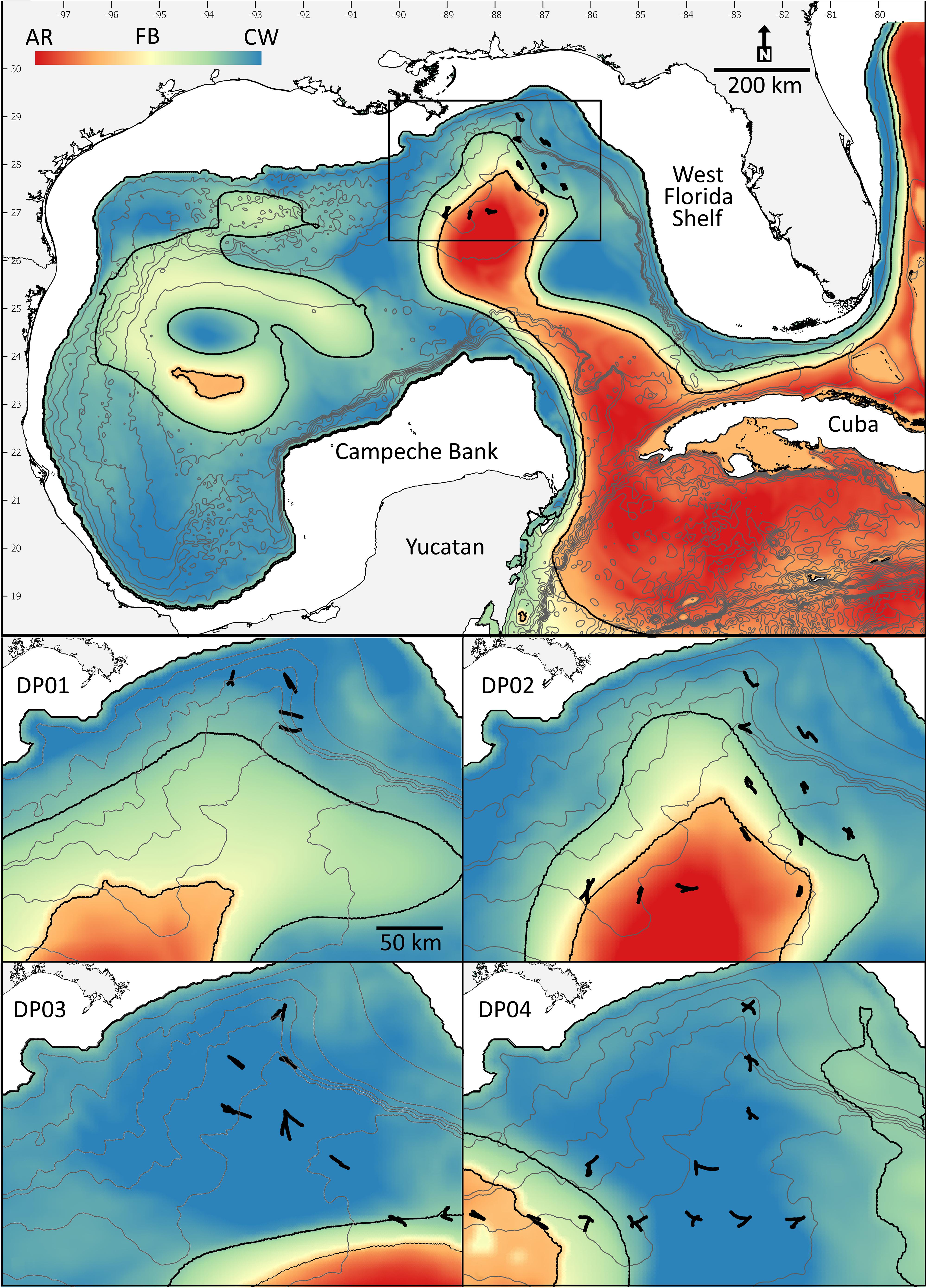
Figure 1. Survey locations (filled symbols) overlaid on the feature classification map illustrating the gradients among the three primary features examined (Loop Current-origin water = red; frontal boundary = green; Gulf Common Water = blue). Lower panels represent survey tracks during each cruise (DP01–DP04). Contour lines represent 500 m depth intervals.

Acoustic Data Collection and Processing

Acoustic data were collected during the day and nighttime periods (defined by local sunrise and sunset) when the transducer was deployed, allowing for continuous surveys (∼8 h) during each transect at each station. A multiple-frequency echosounder system (Simrad EK60/Simrad EK80) was used and operated transducers at 18, 38, 70, 120 kHz. The transducers were mounted in a faring and suspended 2.5 m below the water surface. Given the limitations of using a pole-mounted system, transects were conducted at an approximate vessel speed of 2 knots. Transducers were calibrated according to the standard sphere method (Demer et al., 2015). For this paper, we examined the acoustic backscatter from the sound scattering layers using only the 38 kHz frequency due to: the widespread use of this frequency to study pelagic biomass (Davison et al., 2013; D’Elia et al., 2016; Aksnes et al., 2017; Kaartvedt et al., 2017), the complicating factor of resonance effects from gas-bearing organisms at 18 kHz, and low signal-to-noise ratios in the higher frequencies (70, 120 kHz) (Godø et al., 2009; Fennell and Rose, 2015; Davison et al., 2015). The pulse duration for 38 kHz echosounder was 4 ms with a power setting of 2000 W, and ping repetition rate of 0.2 pings s^–1. Sound speed profiles and absorption coefficient were computed from bin-averaged CTD data using the Ocean Toolbox (McDougall and Barker, 2011) in Matlab.

Raw acoustic backscatter data were imported and manually scrutinized in Echoview (v8, Myriax). Data from the transducer face to 15 m depth were excluded from the analysis to account for beam formation and to eliminate surface-associated interference (e.g., bubble sweep down). Data beyond 1000 m were not included in the analysis due to range dependent losses in attenuation and signal strength. Compromised data due to interference from other shipboard sonar systems (intermittent or spike noise), false bottom, and background noise were excluded from the analysis. False bottoms were manually excluded. To remove occurrences of spike noise, each sample was compared to the preceding and successive sample. If the single ping-to-ping difference was greater than 10 dB the sample was considered a spike candidate and replaced with the mean S_V of four neighboring samples (D’Elia et al., 2016). Background noise was identified and removed following a modified process described by De Robertis and Higginbottom (2007). A minimum signal-to-noise ratio of 15 dB was applied to data collected at 38 kHz. Samples that did not satisfy this threshold were considered indistinguishable from the background noise and flagged as ’no data.’ The measurements of Nautical Area Scattering Coefficient (NASC; m² nmi^–2) were derived from the echo integral in 500-m along-track x 5-m vertical bins with a −80 dB re 1 m² integration threshold (MacLennan et al., 2002). NASC is considered to be proportional to the abundance of biological scatterers and serves as a comparable index of organism biomass (Hazen et al., 2009; Zwolinski et al., 2010; Fennell and Rose, 2015). Integrated backscatter was further binned into three depth intervals: 15–200 m (epipelagic), 200–600 m (upper mesopelagic) and 600–1000 m (lower mesopelagic). The center of mass (m) was derived for each of the three depth intervals using the approach of Urmy et al. (2012) to describe depth of the statistical center of the backscatter within each depth interval.

Oceanographic Feature Identification Methods

Oceanographic feature classes were identified following Johnston et al. (2019); these include Loop Current-origin water (LCOW), Gulf Common Water, and frontal boundaries. These feature classes were derived from the GoM HYbrid Coordinate Ocean Model (HYCOM + NCODA Gulf of Mexico 1/25° Analysis, GoM l0.04/expt_32.5) (Chassignet et al., 2007), which is a three-dimensional, eddy-resolving circulation model that assimilates satellite- and in situ-derived measures to depict ocean conditions (e.g., sea surface height, zonal velocity, meridional velocity, temperature, and salinity) in near real time, from surface waters to the benthos. In the GoM, HYCOM data are available at 1/25° (c. 4 km²) horizontal resolution, in hourly intervals from 1993 to the present day¹ (Johnston et al., 2018, 2019). Velocity fronts were calculated as the difference between the minimum and maximum water speed within a 0.10 arc degree radius (∼11 km) of each location, derived from the HYCOM and measured in m s^–1.

LCOW is generally characterized by increased SSHA, increased water temperatures (extending down to ca. 1000 m), and a reduction in surface water chlorophyll concentrations. Based on the values used in Johnston et al. (2019), we derived an index that normalized the response of the LCOW and represented a derived quantity that utilized location-specific HYCOM output, given the equation:

$$\mathrm{LCOW}\mathrm{index}=\mathrm{SSHA}{}_{\mathrm{i}}-(\mathrm{SSHA}{}_{\mathrm{GOM}}+0.067)+T{}_i-15.922(1)$$

where SSHA_i represents the location-specific SSHA, SSHA_GOM is the daily mean SSHA in the GoM and T_i represents the location-specific temperature at 300 m. The output from Eq. 1 was scaled between 1.0 and 2.0, where 1.0 is the weakest condition and 2.0 represents the most intense condition measured for the entire GoM. The LCOW index. As such, the lower SSHA threshold for LCOW is SSHA_GOM + 0.067 m and the lower temperature threshold for the is 15.92°C, following Johnston et al. (2019).

Gulf Common Water is generally characterized by decreased SSHA and water column temperature and increased surface water chlorophyll concentrations when compared to LCOW. An index was computed for Gulf Common Water as the difference between the Johnston et al. (2019) temperature threshold at 300 m depth (13.46°C) and the location specific temperature at 300 m – i.e., the colder the water at 300 m, the greater the Gulf Common Water index value. The common water index was normalized to range from 0.0 to −1.0.

Frontal boundaries in the GoM are typically areas where significant mixing between LCOW and Common Water occur. To grade the strength of these boundaries, a frontal boundary index was calculated based on the difference between the SSHA_i and the SSHA_GOM and scaled to range from 0.0 to 1.0, with a value of 1.0 representing conditions nearest LCOW, and 0.0 being closest to Common Water (Johnston et al., 2019).

These oceanographic intensity indices were generated to span as a continuum following the classifications of Johnston et al. (2019) and then standardized and scaled to their respective ranges (i.e., LCOW: 1 to 2; frontal boundary: 0 to 1; Gulf Common Water: 0 to −1) based on the strength of the feature for the duration of the sampled period. Along-track positions for each acoustic survey were then used to extract and quantify the oceanographic conditions for each echo integration cell.

Hydrographic Properties of the Water Column

A calibrated SeaBird CTD (SBE 911+; SeaBird Electronics, Inc.) was used to characterize the water column properties. Data were collected during each night and day period as conditions allowed to characterize the diel structure of the water column. The raw instrument data were processed in the SeaBird processing software (v. 7.23), to compute 1-m bin-averaged estimates of salinity (PSU), temperature (°C), dissolved oxygen concentration (mg L^–1) and chl a (mg L^–1).

Approximating Surface Light Intensity and Primary Production

We examined the effect of relative light availability at 5 m depth by computing the instantaneous photosynthetically active radiation (IPAR; W m^–2) along each transect:

$$IPAR{}_{5m}=IPAR{}_{surf}*2.72{}^{(-Kd(490)*z)}(2)$$

where the surface light intensity IPAR_surf was approximated by NOAA’s Geostationary Satellite Server (GOES); Kd(490) represents NASA’s Moderate Resolution Imaging Spectroradiometer (MODIS) derived diffuse attenuation coefficient at 490 nm, and z represents water depth (5 m). Observations at night have IPAR_surf values of 0. Hourly estimates of solar elevation were derived from NOAA’s Earth System Research Lab². The maximum estimates of solar elevation were 71.4° at local-noon (DP02) and minimum was −65.5° (DP04) at local-midnight (Figure 2). Sixty-day net primary production was compiled from the MODIS observations and estimated from the Vertically Generalized Production Model (Behrenfeld and Falkowski, 1997) made available from the Oregon State Ocean Productivity standard products³. Integrated net primary production estimates were extracted for each cruise (Supplementary Figure S1).

FIGURE 2

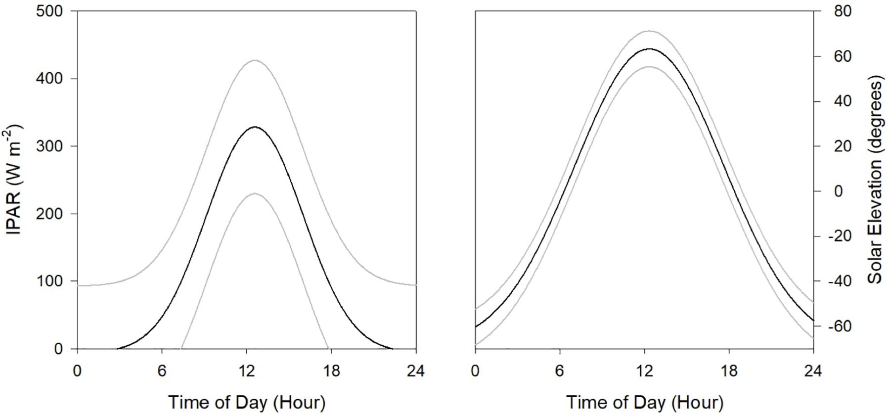
Figure 2. Estimated mean (black line) and 95% confidence intervals (gray lines) of light intensity at 5 m depth (IPAR_5m, left panel) and solar elevation (right panel) across the four surveys conducted in the northern GoM during 2015 and 2016.

Net Collection

Micronekton were sampled with a 10 m² Multiple Opening and Closing Net Sampling System (MOCNESS) conducted synchronously with acoustic data. Briefly, the MOCNESS was used to sample discrete depth intervals from 0 to 1500 m water depth at each station. The MOCNESS was configured with 9 identical nets with 333 μm mesh (see Wiebe et al., 1985 for full system description). Samples were sorted, identified to lowest taxonomic level possible, enumerated, and weighed (either individually or in groups depending on size) onboard the vessel. Organisms were preserved in formalin for long-term storage and later analyses.

Data Analysis

Patterns in acoustic backscatter at 38 kHz (NASC, m² nmi^–2) and the center of mass (m) of sound scattering layers were examined by time of day (day and night), and across the depth intervals (D’Elia et al., 2016). We investigated these patterns relative to the three oceanographic feature classes (LCOW, frontal boundary, and Common Water), using a linear mixed effects model, implemented in R (R Core Team, 2013) with the library “nlme.” Since the variation in the residuals differed by day and night and across the three intervals of depth for both NASC and center of mass, a weighting option was added to the model using the varComb and varIdent structure to allow for different variances by time of day and depth domain. NASC values were log₁₀(x) transformed prior to analysis to meet the assumptions of normality. The responses in log-NASC and center of mass were examined relative to the interactions of time of day, depth interval and feature class. The cruise number was included as random effect to allow the magnitude of NASC and center of mass to vary by cruise. Tukey’s post hoc comparisons were used to identify significant differences with respect to log mean NASC and mean center of mass.

Generalized additive mixed models (GAMMs) were used to analyze the relationships of NASC and center of mass with the environmental and oceanographic drivers for each of the three depth intervals. HYCOM-derived sea surface temperature (°C), HYCOM-derived surface salinity (PSU), CTD-derived maximum chlorophyll concentration, and an index representing the gradient of the oceanographic feature classes were included as main effects. We also examined the interactions of surface (5 m) light intensity and the feature class indices as differences in light intensity at depth would be mediated by factors at the surface and likely reflect oceanographic differences.

Generalized additive mixed models were implemented with the “mgcv” library in R using a Gaussian distribution with an identity link function. Model selection was conducted using a null space penalization. To avoid overfitting, the spline fitting process of the main effect was restricted to 5 knots within the GAMM. We included the survey in the model as a random factor. In addition, the varIdent function was inserted as a weighting factor to allow for variance in fit between day and night. A Spearman’s correlation matrix was calculated to determine collinearity among the environmental variables. Variables used in the model were selected by using a cut off value of 0.80. The autocorrelation of residuals was modeled using a first-order autoregressive error structure nested within each deployment.

Results

Properties of Sound Scattering Layers

Acoustic backscatter intensity (log₁₀ NASC) varied among the three feature classes, time of day, and across the three depth intervals. Within the epipelagic (15–200 m), acoustic backscatter intensity was significantly greater during the night among all feature types (p < 0.001), with values greater by a factor of 25-fold in frontal boundaries, 17-fold in LCOW, and 12-fold in Common Water, relative to daytime values (Table 1). During both nighttime and daytime, the lowest backscatter occurred within the LCOW (Figure 3). Daytime backscatter increased significantly (p < 0.001) from the LCOW to frontal boundaries, and from frontal boundaries to Common Water. However, at night backscatter was greatest within the frontal boundaries and slightly less, although not significantly, (p = 0.258), within Common Water. Similarly, within the upper mesopelagic (200–600 m), acoustic backscatter increased significantly (p < 0.001) from LCOW to frontal boundaries, and from frontal boundaries to Common Water during the day; however, LCOW and frontal boundary features displayed significantly greater backscatter (p < 0.001) at night than Common Water (Figure 3). In contrast to the other two depth intervals, lower mesopelagic zone (600–1000 m) LCOW waters had significantly (p < 0.001) greater backscatter than the same depth interval in either frontal boundary or Common Water, with nearly a 9-fold and 19-fold increase relative to the latter two features at night, respectively (Figure 3).

TABLE 1

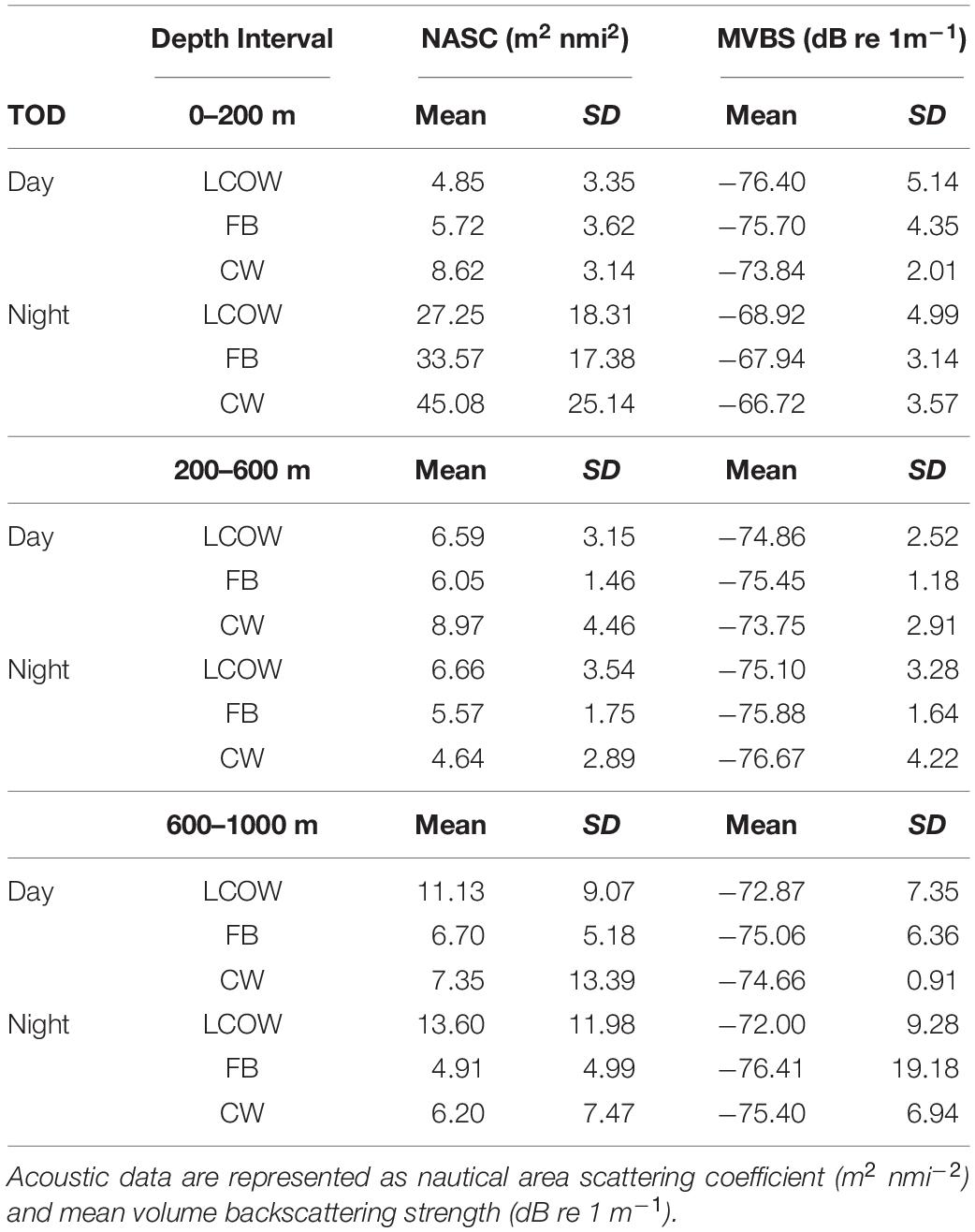
Table 1. Mean acoustic backscatter by time of day (TOD) and oceanographic feature class (LCOW, Loop Current-origin water; FB, Frontal boundary; CW, Common Water).

FIGURE 3

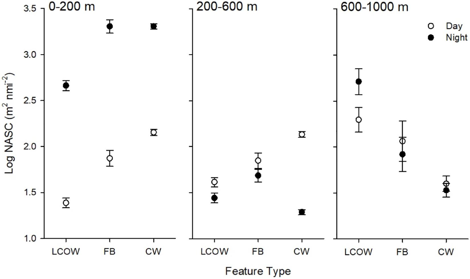
Figure 3. Least-squared means of acoustic backscatter, log₁₀ NASC (m² nmi^–2), by feature class, time of day (open symbols are day, filled are night) and depth interval. LCOW, Loop Current-origin water; FB, frontal boundary; and CW, Gulf Common Water. Error bars represent standard error from least-squared mean estimates.

In all cases, during the day the center of mass occurred significantly deeper in frontal boundaries than in LCOW, and in Common Water than frontal boundaries (p < 0.001; Figure 4); however, at night the responses were more variable. At night the center of mass within the LCOW was consistently and significantly (p < 0.001) deeper than within frontal boundaries and Common Water. Within the epipelagic zone the centers of mass of frontal boundaries and Common Water were significantly shallower than within LCOW (p < 0.001). The centers of mass within the upper mesopelagic occurred deepened going from LCOW to frontal boundaries to Common Water, respectively (p < 0.001) (Figure 4). The location of the centers of mass within the lower mesopelagic zone was the most variable at night, with frontal boundaries having a significantly shallower center of mass (716.7 m; p < 0.001) than either Common Water (737.7 m) or LCOW (766.2 m) (Figure 4).

FIGURE 4

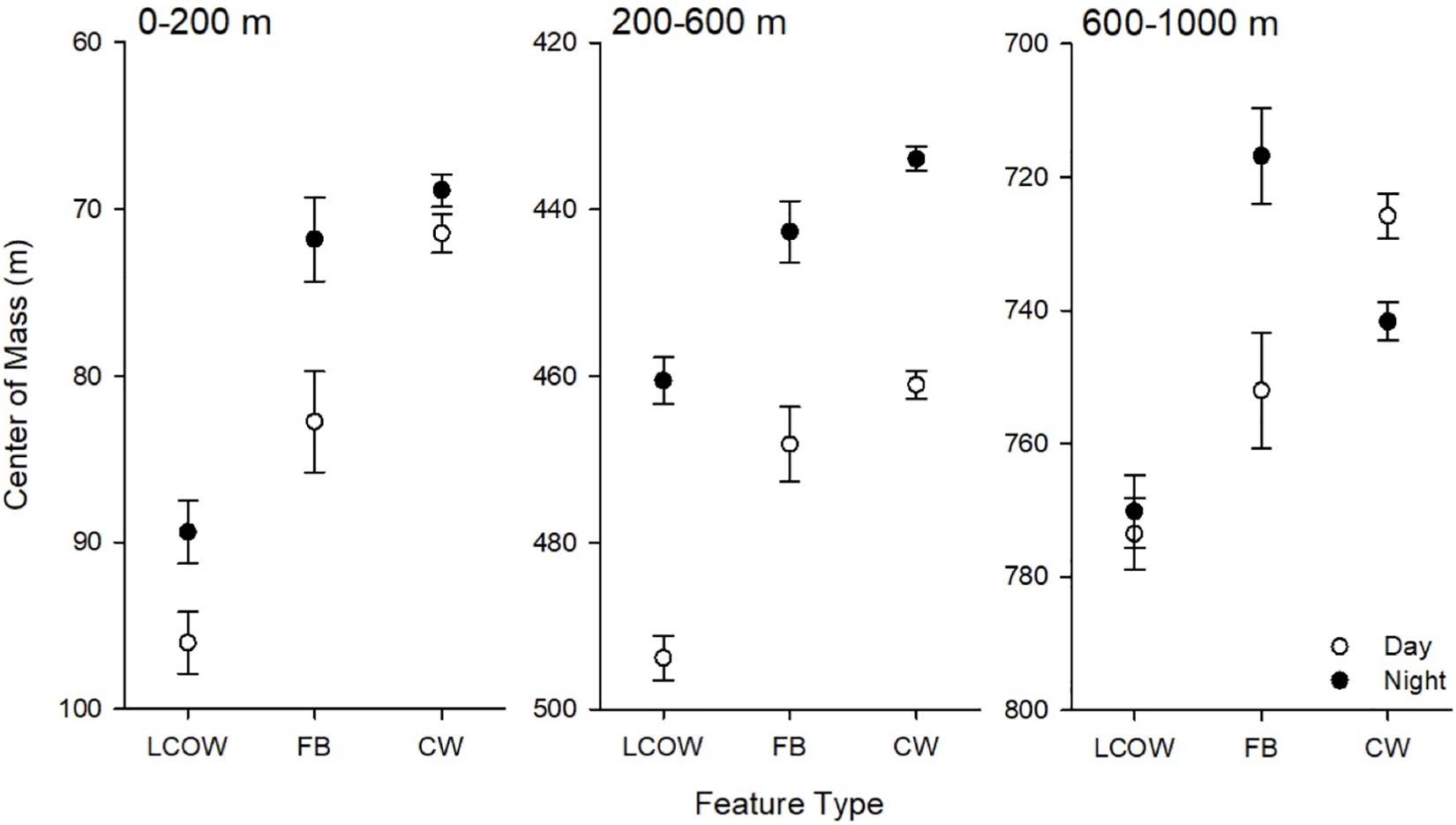
Figure 4. Least-squared means of center of mass by feature class, time of day (open symbols are day, filled are night) and depth interval. LCOW, Loop Current-origin water; FB, frontal boundary; and CW, Gulf Common Water. Error bars represent standard error from least-squared mean estimates.

Effect of Environmental Drivers on Backscatter

Surface light intensity (IPAR; W m^–2) at 5 m water depth was not significantly different among the three oceanographic feature classes (Kruskal–Wallis One Way ANOVA on Ranks, p = 0.765); although in general LCOW stations displayed greater surface light intensity, followed by frontal boundaries and Common Water (Figure 5). In all GAMMs light intensity and the LCOW index emerged as the most consistently significant variables (Supplementary Table S1) among all three depth intervals. Temperature, chlorophyll and the Common Water index were significant variables with respect to backscatter in certain cases (Supplementary Tables S1, S2). With the exception of only a few stations in cruises DP01 and DP02, transects were seaward of the coastal production plume associated with the Mississippi River, where net primary production exceeded 700 mg C m^–2 d^–1 (Supplementary Figure S1). Below we discuss the significant interactions between the oceanographic index scores and light intensity with backscatter across the three depth intervals.

FIGURE 5

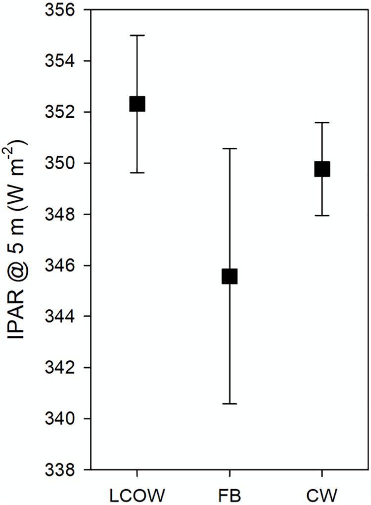
Figure 5. Mean surface light intensity (IPAR) at 5 m water depth for each of the three oceanographic feature classes surveyed during DP01–DP04. LCOW, Loop Current-origin Water; FB, frontal boundary; and CW, Gulf Common Water. Error bars represent standard error of the mean.

Within the epipelagic, the acoustic backscatter was correlated with surface light intensity, sea surface temperature, chlorophyll concentration, and the LCOW index, as well as the interaction between light intensity and the LCOW index (r² = 0.53; Supplementary Table S1). The partial plots indicated an increasing trend in backscatter at light intensity values < 200 W m^–2 (local night). As expected, backscatter decreased in the epipelagic as light levels increased beyond 200 W m^–2, ostensibly a function of DVM. In addition, backscatter decreased as surface temperature increased. Increased surface chlorophyll concentrations were associated with increased backscatter (Supplementary Table S1). As the intensity of the LCOW index increased in the epipelagic, we observed precipitous declines in backscatter, with a nearly 45% decline at night. In the epipelagic, only the LCOW index and light intensity interaction was significant (p < 0.001; Figure 6).

FIGURE 6

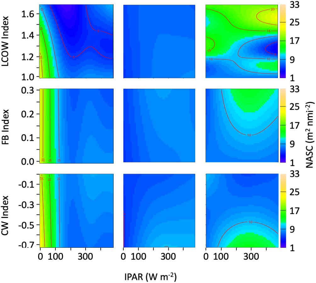
Figure 6. Heatmap representing acoustic backscatter (NASC) as a function of the oceanographic index and light intensity (IPAR_5m). (Left panels) Represent the epipelagic (15–200 m), (center panels) represent upper-mesopelagic (200–600 m), and (right panels) represent lower mesopelagic (600–1000 m).

In the upper mesopelagic, light intensity was the most significant factor (p < 0.001) explaining variance in backscatter intensity, with lesser explanatory power attributed to the Common Water index (p = 0.004), the interaction of the Common Water index with light intensity (Supplementary Table S1). A decrease in backscatter was associated with increasing values of the Common Water index (p = 0.004) and with decreasing light intensity (p < 0.001) (Supplementary Table S1). During daytime and nighttime, a decrease in backscatter was observed with a greater LCOW index, whereas lower values of the Common Water index were associated with increased backscatter during the day (Figure 4). In general, the correlation of backscatter and light intensity within the upper mesopelagic was less variable than either epipelagic or lower mesopelagic depths.

Backscatter within the lower mesopelagic was significantly related to the velocity of the front, the LCOW index, and the interaction of light intensity in both LCOW and Common Water stations (Supplementary Table S1). The interaction of light intensity and the Common Water and LCOW indices were significant at depths greater than 600 m, with an increase in backscatter during the day at the lowest values of the Common Water index (Figure 6), and greater backscatter during the day and night periods for higher LCOW index (Figure 6).

Vertical Distribution of Backscatter

The GAM model for the center of mass indicated that within the epipelagic zone the vertical distribution of sound scattering layers were significantly related only to the maximum chlorophyll concentration (p < 0.001; r² = 0.16; Supplementary Table S2), suggesting a deepening of the center of mass as chlorophyll concentration increases.

The model for the upper mesopelagic was significant (p < 0.001; r² = 0.33) and selected six terms explaining variability in the center of mass: light intensity, temperature, salinity, maximum chlorophyll concentration, LCOW index and the interaction between the latter and the light intensity (Supplementary Table S2). The effect of light intensity on the center of mass indicated that biomass was deeper in the day and shallower at night, while an increase in sea surface temperature, salinity, and the LCOW index were associated with a deeper center of mass. In contrast, the center of mass was shallower with increases in the maximum chlorophyll concentration (Supplementary Table S2).

Within the lower mesopelagic, the center of mass was significantly related to the LCOW index (p < 0.001) in addition to the surface temperature (p < 0.001) and surface salinity (p = 0.003). A strong relationship was observed with the LCOW index, suggesting that as the LCOW index increases, the center of mass of layers gets deeper. The deepening of the center of mass occurred both during day and nighttime as indicated by the significant interaction between light intensity and LCOW index (p = 0.02) (Supplementary Table S2).

Biological Ground Truthing

Detailed information on the faunal composition, vertical distribution, and standing stocks of the epi- and mesopelagic fauna collected during DEEPEND surveys are reported elsewhere (Judkins et al., 2016; Burdett et al., 2017; Sutton et al., 2017; Frank et al., 2020; Judkins and Vecchione, 2020; Milligan and Sutton, 2020), but will be briefly summarized here. The two dominant taxonomic groups collected with the MOCNESS were fishes and macrocrustaceans (large euphausiids, decapod shrimps, mysids, lophogastrids). Macrocrustaceans were the most abundant group by number, contributing 26.5% of the total abundance of organisms collected, with euphausiids being numerically dominant (e.g., Nematoscelis atlantica, Stylocheiron abbreviatum, and Thysanopoda obtusifrons). The fish assemblage was dominated by the Order Stomiiformes (75% of all fishes collected; Sutton et al., 2020), particularly species of the genus Cyclothone which contributed 18.7% by number of all organisms collected (fishes and invertebrates). The species Cyclothone pallida accounted for over half (56%) of this dominant genus. Myctophid species often dominated the numbers of upper mesopelagic layers and the epipelagic layer at night (Sutton et al., 2017, 2020; Milligan and Sutton, 2020). Other taxa commonly collected in net samples included: gelatinous zooplankton (e.g., siphonophores, medusae, and pyrosomes), shelled pteropods, cephalopods, and a wide variety of “other fishes” (Aulopiformes, Stephanoberyciformes, early life stages of coastal and benthic taxa; Sutton et al., 2017, 2020). In relation to water mass, LCOW and Common Water stations had the greatest number of individuals from net collections, with 40 and 44%, respectively. Each had similar species composition, dominated by the macrocrustaceans and fishes mentioned above.

Discussion

Horizontally continuous sound scattering layers were ubiquitous in the northern GoM, throughout all periods and features surveyed in this study, occupying all three depth intervals examined. As expected, an increase in acoustic backscatter was observed during periods of low surface light intensity (<200 W m^–2) in the epipelagic, followed by a coincident decrease in upper mesopelagic backscatter at night due to the upwardly migrating mesopelagic assemblage. This pattern was observed consistently across all oceanographic feature classes.

Sound Scattering Layer Response to Oceanographic Features

In general, LCOW stations were characterized by the lowest backscatter intensity within the epipelagic, intermediate intensity in the upper mesopelagic, and greatest in the lower mesopelagic zone. An overall reduction in biomass within anticyclones has been reported across many systems, though the manifestations appear to be system-specific (Godø et al., 2012; Béhagle et al., 2014; Fennell and Rose, 2015; Gaube et al., 2018; but see Goldthwait and Steinberg, 2008). The reduction in lower trophic-level (e.g., zooplankton) biomass associated with anticyclonic features, which are similar in structure to LCOW (Johnston et al., 2019), has been observed previously in the northern GoM (Zimmerman and Biggs, 1999; Wormuth et al., 2000; Ressler and Jochens, 2003; Gasca, 2004) as well as in other low-latitude oceanic regions (Huggett, 2014; Lebourges-Dhaussy et al., 2014). In comparison, Godø et al. (2012) observed variation (∼20 dB re 1 m^–1) in backscatter while transiting across oceanographic discontinuities in the Icelandic Basin, including an anticyclonic eddy. However, they noted patchiness in the biomass estimated across those features. In contrast, Fennell and Rose (2015) demonstrated increased backscatter in mesopelagic sound scattering layers in the mid-North Atlantic Ocean associated with mesoscale anticyclonic eddies and attributed the increased backscatter to transport mechanisms associated with eddy fields. While many studies have noted that cold-core cyclonic eddies, characterized by centrally upwelled, nutrient-enriched water, promote increased primary and secondary productivity in the epipelagic (Biggs, 1992; Zimmerman and Biggs, 1999; Seki et al., 2001; Landry et al., 2008), during our survey periods we did not encounter any such biomass enhancement with respect to higher trophic levels due to the ephemeral nature and/or our undersampling of cyclonic features.

Given the pattern of reduced backscatter (and by proxy, micronekton biomass) in Loop Current and anticyclonic features, two ecological explanations can be proposed: (1) these features support less micronekton biomass as a quasi-self-contained habitat unit, or (2) these features influence avoidance behavior of vertical migrators. Of these explanations, we posit that the second is more likely. First, with respect to in situ production, the known generation times of micronekton are longer than the lifespans of shed Loop Current eddies (e.g., Gartner, 1991) and much longer than cyclonic eddies, which are smaller and more ephemeral than Loop Current eddies (Johnston et al., 2019). This differentiates results found for zooplankton and micronekton – the former can be “spun down” within the lifetime of an anticyclonic eddy due to lack of new production as food resources are exhausted. Second, with respect to spatial coherence of micronekton within a mesoscale feature, differential lateral advection from the surface to depth during vertical migration would be a diffusing agent (Milligan and Sutton, 2020). For micronekton to retain spatial coherence with a mesoscale feature, which is itself in motion, micronekton would have to “track” surface features during the daytime while at depth, although the extent of this effect would be dependent on how deep these features propagate at depth. The classical paradigm of daytime behavior of vertically migrating micronekton is that they are quiescent, conserving energy between feeding bouts, not actively tracking features geographically (Sutton, 2013).

Perhaps the reduction of vertical migration into the epipelagic and upper mesopelagic zones at night under LCOW results in a deep accumulation of biomass in the lower mesopelagic under anticyclonic-like conditions relative to the other two oceanographic features. This supposition would support the behavioral argument posited above. Given that the influence of anticyclonic features can be detected well into, and at times below, the 600–1000 m depth interval (Godø et al., 2012; Furey et al., 2018), it is not surprising to see a response in the sound scattering layers. In our case we detected not only an increase in biomass, but also deepening of the layers associated with LCOW.

The effects of frontal boundaries in surface waters can be highly variable with respect to spatial extent, intensity, and persistence (Belkin et al., 2009), and can therefore have variable effects on aggregating biological resources concentrated through entrainment (Owen, 1981) in addition to larger predators that exploit these hotspots (Bakun, 2006; Scales et al., 2014). The greatest acoustic backscatter was observed at night within frontal boundaries. While Loop Current eddies may be associated with reduced productivity, frontal margins of these features are known to be sites of increased faunal abundance/biomass, for example larval and juvenile fishes (Mohan et al., 2017), and may potentially offset the reduced faunal abundance/biomass observed in the adjacent LCOW.

At some sites, backscatter intensity was not conserved between day and night sampling periods. There are multiple explanations for why this may occur, including the advection of organisms into or out of the study region between sampling intervals or organisms’ target strength varying as a function of depth (which is highly probable for resonant scatterers such as swim-bladders in fish). The fact that backscatter varied over diel periods at some sites and not as much at others presents a challenge in terms of interpreting acoustically measured biomass for migrating organisms, unless light cycle (or time of day) is controlled for in the analysis.

Variation in Depth Distribution

An increase in depth of the sound scattering layers as a function of anticyclonic physics is consistent with downwelling processes characteristic of these features (Carton et al., 2010; Chelton et al., 2011). The estimates of the depth of the center of mass suggest that in LCOW, the sound scattering layers are distributed at greater depths at night and that important biophysical interactions may influence the vertical distribution of the layers through either direct action (i.e., downwelling of migrators and/or their planktonic food) or through influences on individual behavior (migration choice) (Pearre, 2003). Moreover, the interaction between the LCOW index and backscatter suggests that an upper threshold in the oceanographic conditions (indicated by a high LCOW index) might mediate how organisms move into the epipelagic at night (as illustrated in Figure 6). This deepening of the sound scattering layers may indicate that organisms inhabiting these features may remain deeper to avoid the dynamic Loop Current waters, possibly because the current’s hydrodynamics add an additional energetic burden that could contribute to a reduction in the vertical movement of the mesopelagic assemblage. Alternatively, the persistent sound scattering layer detected at depth during the day and night may be attributed in part to both asynchronous migration strategies and non-migrators that continuously remain at depth (Sutton and Hopkins, 1996a; Watanabe et al., 1999; Olivar et al., 2012; Sutton, 2013). The phenomenon of asynchronous migration has been observed across many oceanic systems (Clarke, 1974; Badcock and Merrett, 1976; Kenaley, 2008) including the GoM (Sutton and Hopkins, 1996a, b) where dragonfishes (Stomiidae), the dominant mesopelagic predatory fishes, split their time between the epipelagic and mesopelagic depth intervals at night (Sutton and Hopkins, 1996b). Summaries of MOCNESS data (Sutton et al., 2017; Milligan and Sutton, 2020) indicate that these migration strategies are commonplace among the dominant GoM fish species and that is likely to explain at least in part, the persistent sound scattering layers observed at depth.

Influence of Light Regimes

Light level consistently correlated with temporal patterns in the mesopelagic sound scattering layers. We observed predictable patterns in the way the mesopelagic assemblage responded, with consistent increases in backscatter at night in the epipelagic and mesopelagic. Other studies have demonstrated that light intensity is important for controlling the extent of vertical movement and timing (Frank and Widder, 1997; Aksnes et al., 2017; Kaartvedt et al., 2017). While we were unable to empirically measure the light intensity at depth during this study, our results suggest that predicted light intensities from surface-derived estimates can be used as a predictor variable when direct measurements are unavailable. While others have quantitatively examined the animal response to subtle changes in light intensity (Frank and Widder, 1997; Aksnes et al., 2017; Kaartvedt et al., 2017), our estimates are appropriate to examine an integrated timescale that broadly represents the patterns observed with the DVM of the mesopelagic community. Additionally, while we were able to derive satellite-based estimates of light intensity across the three types of water masses examined, it remains unknown how variability in water transparency in LCOW, frontal boundaries and Common Water might differentially mediate light transmission to the mesopelagic region and in particular, whether the estimates we derived could result in significant differences among the three oceanographic feature classes we examined off the continental shelf.

Implications for Trophic Transfer

While we observed differences in backscatter distribution and intensity across the oceanographic conditions studied, the composition of organisms was not substantially different with net catches being dominated by crustacean macrozooplankton, namely euphausiids (e.g., Nematoscelis atlantica, Stylocheiron abbreviatum, and Thysanopoda obtusifrons), as well as fishes dominated by Cyclothone spp., dominant myctophid species (Sutton et al., 2020; Milligan and Sutton, 2020), other gonoistomatids, and hatchetfishes. An exception was noted for species composition of net hauls at frontal boundary stations, where euphausiids and pteropods were more abundant than fishes (Sutton et al., 2017). This suggests that the variation observed in backscatter is likely attributed in large part to the changes in organismal abundance and vertical distribution rather than a significant change in assemblage structure.

The differences in vertically migrating biomass among oceanographic feature types can have important implications for mediating the strength of trophic interactions and ultimately carbon transfer. Hopkins et al. (1996) estimated that 80% of all trophic exchange within the upper 1000 m of the water column in the eastern GoM (within our study area) occurs within the epipelagic zone at night. These authors determined that this consumption was driven by three dominant fish families (Myctophidae, Sternoptychidae and Gonostomatidae). Based on this study, the reduction in backscatter in LCOW suggests that the Loop Current and its associated eddies are likely areas of reduced trophic exchange, which has important implications for spatially explicit models of the GoM, and by proxy, other large marine ecosystems. Given that Loop Current eddies are persistent and dominant features within the GoM, occupying 100’s of square kilometers and with lifespans exceeding a year, the systematic reduction in trophic transfer likely decreases carbon sequestration by the system as a whole (Volk and Hoffert, 1985; Irigoien et al., 2014; Davison et al., 2015). As reported by Volk and Hoffert (1985), nearly 70% of carbon transport in the upper 1000 m is mediated by the biological pump due to the vertically integrated food web, consequently transporting surface production into the deep ocean (Ducklow et al., 2001; Irigoien et al., 2014; Ariza et al., 2015; Davison et al., 2015).

Conclusion

We demonstrate that Loop Current-origin waters in the upper GoM are associated with decreased acoustic backscatter in comparison to the other oceanographic feature classes examined. These patterns were temporally consistent, suggesting that this oceanographic milieu dampens vertical migration by the mesopelagic assemblage. Perhaps equally important, we demonstrate that within the adjacent frontal boundaries along the margins of Loop Current eddies, increased backscatter was measured in both the epipelagic and mesopelagic at night, and we speculate that this enhancement may offset some portion of the reduced standing stocks observed within the nearby LCOW features.

Physical forcing is an important process that operates at various temporal and spatial scales and can act to structure the distribution of organisms and therefore their roles in ecosystems. In this study, we show that in addition to the previously reported relationship in sound scattering layer dynamics relative to light levels (Røstad et al., 2016; Aksnes et al., 2017), we observed a quantifiable correlation with mesoscale oceanographic features, and the nature of this latter correlation is depth-stratum-specific. Given the ubiquitous distribution, immense biomass, and critical role that migrating sound scattering layers play in the global biological pump, understanding how oceanographic processes mediate the distributional patterns of billions of tons of mesopelagic micronekton is necessary to refine global carbon models (sensu Proud et al., 2017). This is especially true of low-latitude, deep-pelagic ecosystems, which are by far the largest component of the World Ocean. With increases in ocean temperature, and associated ecosystem changes (e.g., expanding oxygen minimum zones; Aksnes et al., 2017), particularly in the marginal seas, approaches that leverage the benefits of large-scale observational techniques with fine-scale, process-based methods provide an efficient means to examine the physical dependencies on biological organization in oceanic systems.

Data Availability Statement

Data are publicly available through the Gulf of Mexico Research Initiative Information and Data Cooperative (GRIIDC) at https://data.gulfresearchinitiative.org (HYCOM 10.7266/N7QR4VK0; Classifications from Johnston et al. (2019) 10.7266/N7QR4VK0; DP01 acoustic data: 10.7289/V5WD3XJS; DP02 acoustic data: 10.7289/V5RN35TF; DP03 acoustic data: 10.7289/V5WD3XSX; and DP04 acoustic data: 10.7289/V5RN3620).

Author Contributions

KB and JW collected the data. KB, MD’E, JM, and JW performed the analysis. All authors contributed to data interpretation and manuscript writing.

Funding

This research was made possible by a grant from The Gulf of Mexico Research Initiative.

Conflict of Interest

The authors declare that the research was conducted in the absence of any commercial or financial relationships that could be construed as a potential conflict of interest.

Acknowledgments

We thank the captain and crew of the R/V Point Sur for their incredible support during the DEEPEND research program and at-sea operations. We appreciate the efforts of the National Centers for Environmental Information (www.ncei.noaa.gov) for assistance with archiving the acoustic data from all the DEEPEND cruises. We thank B. Penta and S. deRada at the Naval Research Lab for access to the high-resolution GoM HyCOM model output as well as C. Hu and the Optical Oceanography Laboratory at the University of South Florida for light intensity data included in the analysis. We thank S. Labua and D. Correa for assistance with data organization and processing and appreciate the comments of the two reviewers that improved this manuscript. This is contribution #176 from the Division of Coastlines and Oceans in the Institute of Environment at Florida International University.

Supplementary Material

The Supplementary Material for this article can be found online at: https://www.frontiersin.org/articles/10.3389/fmars.2020.00051/full#supplementary-material

Footnotes

1. ^ Publicly available at: http://hycom.org.
2. ^ https://www.esrl.noaa.gov/gmd/grad/solcalc/azel.html
3. ^ http://www.science.oregonstate.edu/ocean.productivity/

References

Aksnes, D., Dupont, N., Staby, A., Fiksen, O., Kaartvedt, S., and Aure, J. (2009). Coastal water darkening and implications for mesopelagic regime shifts in Norwegian fjord. Mar. Ecol Press Ser. 387, 39–49. doi: 10.3354/meps08120

CrossRef Full Text | Google Scholar

Aksnes, D., Røstad, A., Kaartvedt, S., Martinez, U., Duarte, C., and Irigoien, X. (2017). Light penetration structures the deep acoustic scattering layers in the global ocean. Sci. Adv. 3:e160246. doi: 10.1126/sciadv.1602468

PubMed Abstract | CrossRef Full Text | Google Scholar

Ariza, A., Garijo, C., Landeira, J. M., Bordes, F., and Hernández-León, S. (2015). Migrant biomass and respiratory carbon flux by zooplankton and micronekton in the subtropical northeast Atlantic Ocean (Canary Islands). Progr. Oceanogr. 134, 330–342. doi: 10.1016/j.pocean.2015.03.003

CrossRef Full Text | Google Scholar

Ariza, A., Landeira, J. M., Escánez, A., Wienerroither, R., Aguilar de Soto, N., Røstad, A., et al. (2016). Vertical distribution, composition and migratory patterns of acoustic scattering layers in the Canary Islands. J. Mar. Syst. 157, 82–91. doi: 10.1016/j.jmarsys.2016.01.004

CrossRef Full Text | Google Scholar

Badcock, J., and Merrett, N. R. (1976). Midwater fishes in the eastern North Atlantic–I. Vertical distribution and associated biology in 30 N, 23 W, with developmental notes on certain myctophids. Progr. Oceanogr. 7, 3–58. doi: 10.11646/zootaxa.3895.3.1

PubMed Abstract | CrossRef Full Text | Google Scholar

Bakun, A. (2006). Fronts and eddies as key structures in the habitat of marine fish larvae: opportunity, adaptive response and competitive advantage. Sci. Mar. 70, 105–122. doi: 10.3989/scimar.2006.70s2105

CrossRef Full Text | Google Scholar

Barham, E. G. (1966). Deep scattering layer migration and composition: observations from a diving saucer. Science 151, 1399–1403. doi: 10.1126/science.151.3716.1399

PubMed Abstract | CrossRef Full Text | Google Scholar

Béhagle, N., Cotté, C., Lebourges-Dhaussy, A., Roudaut, G., Duhamel, G., Brehmer, P., et al. (2017). Acoustic distribution of discriminated micronektonic organisms from a bi-frequency processing: the case study of eastern Kerguelen oceanic waters. Progr. Oceanogr. 156, 276–289. doi: 10.1016/j.pocean.2017.06.004

CrossRef Full Text | Google Scholar

Béhagle, N., du Buisson, L., Josse, E., Lebourges-Dhaussy, A., Roudaut, G., and Ménard, F. (2014). Mesoscale features and micronekton in the Mozambique channel: an acoustic approach. Deep Sea Res. Part IITop. Stud. Oceanogr. 100, 164–173. doi: 10.1016/j.dsr2.2013.10.024

CrossRef Full Text | Google Scholar

Behrenfeld, M. J., and Falkowski, P. G. (1997). Photosynthetic rates derived from satellite-based chlorophyll concentration. Limnol. Oceanogr. 42, 1–20. doi: 10.4319/lo.1997.42.1.0001

CrossRef Full Text | Google Scholar

Behrenfeld, M. J., Gaube, P., Della Penna, A., O’Malley, R. T., Burt, W. J., Hu, Y., et al. (2019). Global satellite-observed daily vertical migrations of ocean animals. Nature 576, 257–261. doi: 10.1038/s41586-019-1796-9

PubMed Abstract | CrossRef Full Text | Google Scholar

Belkin, I. M., Cornillon, P. C., and Sherman, K. (2009). Fronts in large marine ecosystems. Progr. Oceanogr. 81, 223–236. doi: 10.1016/j.pocean.2009.04.015

CrossRef Full Text | Google Scholar

Benoit-Bird, K. J., Moline, M., and Southall, B. (2017). Prey in oceanic sound scattering layers organize to get a little help from their friends. Limnol. Oceanogr. 62, 2788–2798. doi: 10.1002/lno.10606

CrossRef Full Text | Google Scholar

Bertrand, A., Ballón, M., and Chaigneau, A. (2010). Acoustic observation of living organisms reveals the upper limit of the oxygen minimum zone. PLoS One 5:e10330. doi: 10.1371/journal.pone.0010330

PubMed Abstract | CrossRef Full Text | Google Scholar

Bianchi, D., Stock, C., Galbraith, E. D., and Sarmiento, J. L. (2013). Diel vertical migration: ecological controls and impacts on the biological pump in a one-dimensional ocean model. Glob. Biogeochem. Cycles 27, 478–491. doi: 10.1002/gbc.20031

CrossRef Full Text | Google Scholar

Biggs, D. C. (1992). Nutrients, plankton, and productivity in a warm-core ring in the western Gulf of Mexico. J. Geophys. Res. Oceans 97, 2143–2154.

Google Scholar

Boswell, K. (2016). Raw Acoustic Scattering Data Of Organisms from The Water Column, R/V Point Sur, cruise DP01- May 1-8, 2015. Distributed by: Gulf of Mexico Research Initiative Information and Data Cooperative (GRIIDC). Corpus Christi, TX: Harte Research Institute.

Google Scholar

Boswell, K. (2017a). Raw Acoustic Scattering Data Of Organisms From The Water Column, R/V Point Sur, cruise DP02- August 8-21, 2015. Distributed by: Gulf of Mexico Research Initiative Information and Data Cooperative (GRIIDC). Corpus Christi, TX: Harte Research Institute.

Google Scholar

Boswell, K. (2017b). Raw Acoustic Scattering Data Of Organisms From The Water Column, R/V Point Sur, Cruise DP03- April-May, 2016. Distributed by: Gulf of Mexico Research Initiative Information and Data Cooperative (GRIIDC). Corpus Christi, TX: Harte Research Institute.

Google Scholar

Boswell, K. (2017c). Raw Acoustic Scattering Data Of Organisms From The Water Column, R/V Point SUR, CRUise DP04-August 2016. Distributed by: Gulf of Mexico Research Initiative Information and Data Cooperative (GRIIDC). Corpus Christi, TX: Harte Research Institute.

Google Scholar

Brierley, A. (2014). Diel Vertical Migration. Curr. Biol. 24, 1074–1076.

Google Scholar

Brodeur, R. D., Seki, M. P., Pakhomov, E. A., and Suntsov, A. V. (2005). Micronekton - what are they and why are they important? North pacific marine science organization. Pices Press 13, 7–11.

Google Scholar

Burdett, E. A., Fine, C. D., Sutton, T. T., Cook, A. B., and Frank, T. M. (2017). Geographic and depth distributions, ontogeny, and reproductive seasonality of decapod shrimps (Caridea: Oplophoridae) from the northeastern Gulf of Mexico. Bull. Mar. Sci. 93, 743–767. doi: 10.5343/bms.2016.1083

CrossRef Full Text | Google Scholar

Cade, D. E., and Benoit-Bird, K. J. (2015). Depths, migration rates and environmental associations of acoustic scattering layers in the Gulf of California. Deep Sea Res. I 102, 78–89. doi: 10.1016/j.dsr.2015.05.001

CrossRef Full Text | Google Scholar

Cardona, Y., and Bracco, A. (2016). Predictability of mesoscale circulation throughout the water column in the Gulf of Mexico. Deep Sea Res. II Top. Stud. Oceanogr. 129, 332–349. doi: 10.1016/j.dsr2.2014.01.008

CrossRef Full Text | Google Scholar

Carton, X., Daniault, N., Alves, J., Cherubin, L., and Ambar, I. (2010). Meddy dynamics and interaction with neighboring eddies southwest of Portugal: observations and modeling. J. Geophys. Res. 115:C06017. doi: 10.1029/2009JC005646

CrossRef Full Text | Google Scholar

Chassignet, E. P., Hurlburt, H. E., Smedstad, O. M., Halliwell, G. R., Hogan, P. J., Wallcraft, A. J., et al. (2007). The HYCOM (hybrid coordinate ocean model) data assimilative system. J. Mar. Syst. 65, 60–83.

Google Scholar

Chelton, D. B., Schlax, M. G., and Samelson, R. M. (2011). Global observations of nonlinear mesoscale eddies. Prog. Oceanogr. 91, 167–216. doi: 10.1016/j.pocean.2011.01.002

CrossRef Full Text | Google Scholar

Childress, J. J. (1983). Oceanic biology: lost in space. Oceanogr. Present Future 127–135. doi: 10.1007/978-1-4612-5440-9_9

CrossRef Full Text | Google Scholar

Clarke, T. A. (1974). Some aspects of the ecology of stomiatoid fishes in the Pacific Ocean near Hawaii. Fish. Bull. 72, 337–351.

Google Scholar

Davison, P. C., Anthony Koslow, J. A., and Kloser, R. J. (2015). Acoustic biomass estimation of mesopelagic fish: backscattering from individuals, populations, and communities. ICES J. Mar. Sci. 72, 1413–1424. doi: 10.1093/icesjms/fsv023

CrossRef Full Text | Google Scholar

Davison, P. C., Checkley, D. M. Jr., Koslow, J. A., and Barlow, J. (2013). Carbon export mediated by mesopelagic fishes in the northeast Pacific Ocean. Prog. Oceanogr. 116, 14–30. doi: 10.1016/j.pocean.2013.05.013

CrossRef Full Text | Google Scholar

De Robertis, A., and Higginbottom, I. (2007). A post-processing technique to estimate the signal-to-noise ratio and remove echosounder background noise. ICES J. Mar. Sci. 64, 1282–1291. doi: 10.1093/icesjms/fsm112

CrossRef Full Text | Google Scholar

D’Elia, M., Warren, J. D., Rodriquez-Pinto, I., Sutton, T. T., Cook, A., and Boswell, K. M. (2016). Diel Variation in the vertical distribution of deep-water scattering layers in the Gulf of Mexico. Deep Sea Res. I Oceanogr. Res. Pap. 115, 91–102. doi: 10.1016/j.dsr.2016.05.014

CrossRef Full Text | Google Scholar

Demer, D. A., Berger, L., Bernasconi, M., Bethke, E., Boswell, K. M., Chu, D., et al. (2015). Calibration of Acoustic Instruments. ICES Cooperative Research Report No. 326. Copenhagen: ICES, 133.

Google Scholar

Devol, A. H. (1981). Verticaldistributionofzooplanktonrespirationinrelationtothe intense oxygen minimum zones in two British Columbia fjords. J. Plankton Res. 3, 593–602. doi: 10.1093/plankt/3.4.593

CrossRef Full Text | Google Scholar

Drazen, D. C., de Forest, L. G., and Domokos, R. (2011). Micronekton abundance and biomass in Hawaiian waters as influenced by seamounts, eddies and the moon. Deep Sea Res. I Oceanogr. Rese. Pap. 58, 557–566. doi: 10.1016/j.dsr.2011.03.002

CrossRef Full Text | Google Scholar

Ducklow, H. W., Steinberg, D. K., and Buesseler, K. O. (2001). Upper ocean carbon export and the biological pump. Oceanogr. Soc. 14, 50–58. doi: 10.5670/oceanog.2001.06

CrossRef Full Text | Google Scholar

Fennell, S., and Rose, G. (2015). Oceanographic influences on deep scattering layers across the North Atlantic. Deep Sea Res. I Oceanogr. Res. Pap. 105, 132–141. doi: 10.1016/j.dsr.2015.09.002

CrossRef Full Text | Google Scholar

Flock, M. E., and Hopkins, T. L. (1992). Species composition, vertical distribution, and food habits of the sergestid shrimp assemblage in the eastern Gulf of Mexico. J. Crustacean Biol. 12, 210–223. doi: 10.2307/1549076

CrossRef Full Text | Google Scholar

Forward, R. B. Jr. (1976). “Light and diurnal vertical migration: photobehavior and photophysiology of plankton,” in Photochemical and Photobiological Reviews, ed. K. C. Smith (NewYork,NY: PlenumPress), 157–210.

Google Scholar

Frank, T., and Widder, E. (1997). The correlation of downwelling irradiance and staggered vertical migration patterns of zooplankton in Wilkinson Basin, Gulf of Maine. J. Plankton Res. 19, 1975–1991. doi: 10.1093/plankt/19.12.1975

CrossRef Full Text | Google Scholar

Frank, T., Fine, C. D., Burdett, E. A., Cook, A. B., and Sutton, T. T. (2020). The vertical and horizontal distribution of deep-sea crustaceans in the Order Euphausiacea in the vicinity of the Deepwater Horizon oil spill. Front. Mar. Sci. doi: 10.3389/fmars.2020.00099

CrossRef Full Text | Google Scholar

Furey, H., Bower, A., Perez-Brunius, P., Hamilton, P., and Leben, R. (2018). Deep eddies in the Gulf of Mexico observed with floats. J. Phys. Oceanogr. 48, 2703–2719. doi: 10.1175/jpo-d-17-0245.1

CrossRef Full Text | Google Scholar

Gartner, J. V. Jr., Hopkins, T. L., Baird, R. C., and Milliken, D. M. (1987). The lanternfishes (Pisces: Myctophidae) of the eastern Gulf of Mexico. Fish. Bull. U. S. 85, 81–98.

Google Scholar

Gartner, J. V. (1991). Life histories of three species of lanternfishes (Pisces: Myctophidae) from the eastern Gulf of Mexico. Mar. Biol. 111, 11–20. doi: 10.1007/bf01986339

CrossRef Full Text | Google Scholar

Gasca, R. (2004). Distribution and abundance of hyperiid amphipods in relation to summer mesoscale features in the southern Gulf of Mexico. J. Plankton Res. 26, 993–1003. doi: 10.1093/plankt/fbh091

CrossRef Full Text | Google Scholar

Gaube, P., Braun, C. D., Lawson, G. L., McGillicuddy, D. J., Della Penna, A., Skomal, G. B., et al. (2018). Mesoscale eddies influence the movements of mature female white sharks in the Gulf Stream and Sargasso Sea. Sci. Rep. 8:7363. doi: 10.1038/s41598-018-25565-8

PubMed Abstract | CrossRef Full Text | Google Scholar

Gjosaeter, J., and Kawaguchi, K. (1980). A Review of the World Resources Of Mesopelagic Fish. Rome: FAO.

Google Scholar

Godø, O. R., Patel, R., and Pedersen, G. (2009). Diel migration and swimbladder resonance of small fish: some implications for analyses of multifrequency echo data. ICES J. Mar. Sci. 66, 143–148.

Google Scholar

Godø, O. R., Samuelsen, A., Macaulay, G., Patel, R., Hjøllo, S. S., Horne, J., et al. (2012). Mesoscale eddies are oases for higher trophic marine life. PLoS One 7:e30161. doi: 10.1371/journal.pone.0030161

PubMed Abstract | CrossRef Full Text | Google Scholar

Goldthwait, S. A., and Steinberg, D. K. (2008). Elevated biomass of mesozooplankton and enhanced fecal pellet flux in cyclonic and mode-water eddies in the Sargasso Sea. Deep Sea Res. II Top. Stud. Oceanogr. 55, 1360–1377. doi: 10.1016/j.dsr2.2008.01.003

CrossRef Full Text | Google Scholar

Hall, C. A., and Leben, R. R. (2016). Observational evidence of seasonality in the timing of loop current eddy separation. Dyn. Atmos. Oceans 76, 240–267. doi: 10.1016/j.dynatmoce.2016.06.002

CrossRef Full Text | Google Scholar

Handegard, N. O., du Buisson, L., Brehmer, P., Chalmers, S. J., De Robertis, A., Huse, G., et al. (2013). Towards an acoustic-based coupled observation and modelling system for monitoring and predicting ecosystem dynamics of the open ocean. Fish Fish. 14, 605–615. doi: 10.1111/j.1467-2979.2012.00480.x

CrossRef Full Text | Google Scholar

Hazen, E. L., Craig, J. K., Good, C. P., and Crowder, L. B. (2009). Vertical distribution of fish biomass in hypoxic waters on the Gulf of Mexico shelf. Mar. Ecol. Press Ser. 375, 195–207. doi: 10.3354/meps07791

CrossRef Full Text | Google Scholar

Heffernan, J. J., and Hopkins, L. T. (1981). Vertical distribution and feeding of the shrimp genera Gennadas and Bentheogennema (Decapoda: Penaeidea) in the eastern Gulf of Mexico. J. Crustacean Biol. 1, 461–473.

Google Scholar

Herring, H. J. (2010). Gulf of Mexico Hydrographic Climatology and Method of Synthesizing Subsurface Profiles from the Satellite Sea Surface Height Anomaly. ICES Document Report 122. Silver Spring, MD: National Oceanographic and Atmospheric Administration, 63.

Google Scholar

Hidaka, K., Kawaguchi, K., Murakami, M., and Takahashi, M. (2001). Downward transport of organic carbon by diel migratory micronekton in the western equatorial Pacific: it’s quantitative and qualitative importance. Deep Sea Res. I Oceanogr. Res. Pap. 48, 1923–1939. doi: 10.1016/s0967-0637(01)00003-6

CrossRef Full Text | Google Scholar

Hopkins, T., Sutton, T. T., and Lancraft, T. M. (1996). The trophic structure and predation impact of a low latitude midwater fish assemblage. Prog. Oceanogr. 38, 205–239. doi: 10.1016/s0079-6611(97)00003-7

CrossRef Full Text | Google Scholar

Hopkins, T. L., and Lancraft, T. M. (1984). The composition and standing stock of mesopelagic micronekton at 27 N 86 W in the eastern Gulf of Mexico. Mar. Sci. 27, 143–158.

Google Scholar

Hudson, J. M., Steinberg, D. K., Sutton, T. T., Graves, J. E., and Latour, R. J. (2014). Myctophid feeding ecology and carbon transport along the northern Mid-Atlantic Ridge. Deep Sea Res. I Oceanogr. Res. Pap. 93, 104–116. doi: 10.1016/j.dsr.2014.07.002

CrossRef Full Text | Google Scholar

Huggett, J. (2014). Mesoscale distribution and community composition of zooplankton in the Mozambique Channel. Deep Sea Res. II Top. Stud. Oceanogr. 100, 119–135. doi: 10.1016/j.dsr2.2013.10.021

CrossRef Full Text | Google Scholar

Irigoien, X., Klevjer, T. A., Røstad, A., Martinez, U., Boyra, G., Acuña, J. L., et al. (2014). Large mesopelagic fishes biomass and trophic efficiency in the open ocean. Nat. Commun. 5:3271. doi: 10.1038/ncomms4271

PubMed Abstract | CrossRef Full Text | Google Scholar

Johnston, M. W., Milligan, R. J., Easson, C. G., de Rada, S., English, D., Penta, B., et al. (2019). An empirically-validated method for characterizing pelagic habitats in the Gulf of Mexico using ocean model data. Limnol. Oceanogr. Methods 17, 363–375.

Google Scholar

Johnston, M. W., Milligan, R. J., Easson, C. G., deRada, S., English, D., Penta, B., et al. (2018). Habitat classification of the Gulf of Mexico (GOM) using the HYbrid Coordinate Ocean Model (HYCOM) and salinity/temperature profiles, cruises DP01-DP04, May 2015 to August 2016. Distributed by: Gulf of Mexico Research Initiative Information and Data Cooperative (GRIIDC). Corpus Christi, TX: Harte Research Institute.

Google Scholar

Judkins, H. L., Vecchione, M., and Rosario, K. (2016). Morphological and molecular evidence of Heteroteuthis dagamensis in the Gulf of Mexico. Bull. Mar. Sci. 92, 51–57. doi: 10.5343/bms.2015.1061

CrossRef Full Text | Google Scholar

Judkins, H., and Vecchione, M. (2020). Vertical distribution patterns of cephalopods in the northern Gulf of Mexico. Front. Mar. Sci. doi: 10.3389/fmars.2020.00047

CrossRef Full Text | Google Scholar

Kaartvedt, S., Røstad, A., and Aksnes, D. (2017). Changing weather causes behavioral responses in the lower mesopelagic. Mar. Ecol. Press Ser. 574, 259–263. doi: 10.3354/meps12185

CrossRef Full Text | Google Scholar

Kenaley, C. P. (2008). Diel vertical migration of the loosejaw dragonfishes (Stomiiformes: Stomiidae: Malacosteinae): a new analysis for rare pelagic taxa. J. Fish Biol. 73, 888–901. doi: 10.1111/j.1095-8649.2008.01983.x

CrossRef Full Text | Google Scholar

Kinsey, S. T., and Hopkins, T. L. (1994). Trophic strategies of euphausiids in a low-latitude ecosystem. Mar. Biol. 118, 651–661. doi: 10.1007/bf00347513

CrossRef Full Text | Google Scholar

Klevjer, T. A., Irigoien, X., Røstad, A., Fraile-Nuez, E., Benítez-Barrios, V. M., and Kaartvedt, S. (2016). Large scale patterns in vertical distribution and behaviour of mesopelagic scattering layers. Sci. Rep. 6, 1–11. doi: 10.1038/srep19873

PubMed Abstract | CrossRef Full Text | Google Scholar

Kloser, R. K., Ryan, T., Sakov, P., Williams, A., and Koslow, J. A. (2002). Species identification in deep water using multiple acoustic frequencies. Can. J. Fish. Aquat. Sci. 59, 1065–1077. doi: 10.1139/f02-076

CrossRef Full Text | Google Scholar

Kumar, P. V. H., Kumar, T. P., Sunil, T., and Gopakumar, M. (2005). Observations on the relationship between scattering layer and mixed layer. Curr. Sci. 88:1799.

Google Scholar

Kupchik, M. J., Benfield, M. C., and Sutton, T. T. (2018). The first in situ encounter of Gigantura chuni (Giganturidae: Giganturoidei: Aulopiformes: Cyclosquamata: Teleostei), with a preliminary investigation of pair-bonding. Copeia 106, 641–645. doi: 10.1643/ce-18-034

CrossRef Full Text | Google Scholar

Landry, M. R., Decima, M., Simmons, M. P., Hannides, C. C., and Daniels, E. (2008). Mesozooplankton biomass and grazing responses to Cyclone Opal, a subtropical mesoscale eddy. Deep Sea Res. II Top. Stud. Oceanogr. 55, 1378–1388. doi: 10.1016/j.dsr2.2008.01.005

CrossRef Full Text | Google Scholar

Last, K. S., Hobbs, L., Berge, J., Brierley, A. S., and Cottier, F. (2016). Moonlight drives ocean-scale mass vertical migration of zooplankton during the arctic winter. Curr. Biol. 26, 244–251. doi: 10.1016/j.cub.2015.11.038

PubMed Abstract | CrossRef Full Text | Google Scholar

Lebourges-Dhaussy, A., Huggett, J., Ockhuis, S., Roudaut, G., Josse, E., and Verheye, H. (2014). Zooplankton size and distribution within mesoscale structures in the Mozambique Channel: a comparative approach using the TAPS acoustic profiler, a multiple net sampler and ZooScan image analysis. Deep Sea Res. II Top. Stud. Oceanogr. 100, 136–152. doi: 10.1016/j.dsr2.2013.10.022

CrossRef Full Text | Google Scholar

MacLennan, D. N., Fernandes, P. G., and Dalen, J. (2002). A consistent approach to definitions and symbols in fisheries acoustics. ICES J. Mar. Sci. 59, 365–369. doi: 10.1006/jmsc.2001.1158

CrossRef Full Text | Google Scholar

Marshall, N. B. (1954). Aspect of Deep Sea Biology. London: Hutchinson’s Scientific.

Google Scholar

McDougall, T. J., and Barker, P. M. (2011). Getting Started with TEOS-10 and the Gibbs Seawater (GSW) Oceanographic Toolbox. France: SCOR.

Google Scholar

Merrett, N., and Roe, H. S. J. (1974). Patterns and selectivity in the feeding of certain mesopelagic fishes. Mar. Biol. 28, 115–126. doi: 10.1007/bf00396302

CrossRef Full Text | Google Scholar

Milligan, R. J., Bernard, A. M., Boswell, K. M., Bracken-Grissom, H. D., D’Elia, M. A., DeRada, S., et al. (2019). The application of novel research technologies by the deep pelagic nekton dynamics of the Gulf of Mexico (DEEPEND) consortium. Mar. Technol. Soc. J. 52, 81–86. doi: 10.4031/mtsj.52.6.10

CrossRef Full Text | Google Scholar

Milligan, R. J., and Sutton, T. T. (2020). Dispersion overrides environmental variability as a primary driver of the horizontal assemblage structure of the mesopelagic fish family Myctophidae in the northern Gulf of Mexico. Front. Mar. Sci. 7:15. doi: 10.3389/fmars.2020.00015

CrossRef Full Text | Google Scholar

Mohan, J. A., Sutton, T. T., Cook, A. B., Boswell, K. M., and Wells, R. J. D. (2017). Influence of oceanographic conditions on abundance and distribution of post-larval and juvenile carangid fishes in the northern Gulf of Mexico. Fish. Oceanogr. 1, 1–16.

Google Scholar

Olivar, M. P., Bernal, A., Molí, B., Peña, M., Balbín, R., Castellón, A., et al. (2012). Vertical distribution, diversity and assemblages of mesopelagic fishes in the western Mediterranean. Deep Sea Res. I Oceanogr. Res. Pap. 62, 53–69. doi: 10.1016/j.dsr.2011.12.014

CrossRef Full Text | Google Scholar

Owen, R. (1981). Fronts and eddies in the sea: mechanisms, interactions and biological effects. Analy. Mar. Ecosyst. 1, 197–233. doi: 10.1371/journal.pone.0129045

PubMed Abstract | CrossRef Full Text | Google Scholar

Passarella, K. C., and Hopkins, T. L. (1991). Species composition and food habits of the micronektonic cephalopod assemblage in the eastern Gulf of Mexico. Bull. Mar. Sci. 49, 638–659.

Google Scholar

Pearre, S. (2003). Eat and run? The hunger/satiation hypothesis in vertical migration: history, evidence and consequences. Biol. Rev. 78, 1–79. doi: 10.1017/s146479310200595x

PubMed Abstract | CrossRef Full Text | Google Scholar

Peña, M., Olivar, M. P., Balbín, R., López-Jurado, J. L., Iglesias, M., and Miquel, J. (2014). Acoustic detection of mesopelagic fishes in scattering layers of the Balearic Sea (western Mediterranean). Can. J. Fish. Aquat. Sci. 71, 1186–1197. doi: 10.1139/cjfas-2013-0331

CrossRef Full Text | Google Scholar

Potier, M., Marsac, F., Cherel, Y., Lucas, V., Sabatié, R., Maury, O., et al. (2007). Forage fauna in the diet of three large pelagic fishes (lancetfish, swordfish and yellowfin tuna) in the western equatorial Indian Ocean. Fish. Res. 83, 60–72. doi: 10.1016/j.fishres.2006.08.020

CrossRef Full Text | Google Scholar

Proud, R., Cox, M., Wotherspoon, S., and Brierley, A. (2017). Biogeography of the Global Ocean’s Mesopelagic Zone. Curr. Biol. 27, 113–119. doi: 10.1016/j.cub.2016.11.003

PubMed Abstract | CrossRef Full Text | Google Scholar

R Core Team (2013). R: A Language and Environment for Statistical Computing. Vienna, Austria: R Foundation for Statistical Computing, Available at: www.R-project.org.

Google Scholar

Ressler, P. H., and Jochens, A. E. (2003). Hydrographic and acoustic evidence for enhanced plankton stocks in a small cyclone in the northeastern Gulf of Mexico. Continent. Shelf Res. 23, 41–61. doi: 10.1016/s0278-4343(02)00149-8

CrossRef Full Text | Google Scholar

Richards, W. J., McGowan, M. F., Leming, T., Lamkin, J. T., and Kelley, S. (1993). Larval fish assemblages at the loop current boundary in the Gulf of Mexico. Bull. Mar. Sci. 53, 475–537.

Google Scholar

Rivas, D., Badan, A., and Ochoa, J. (2005). The ventilation of the deep Gulf of Mexico. J. Phys. Oceanogr. 35, 1763–1781. doi: 10.1175/jpo2786.1

CrossRef Full Text | Google Scholar

Robertson, K. M., and Chivers, S. J. (1997). Prey occurrence in pantropical spotted dolphins, Stenella attenuata, from the eastern tropical Pacific. Fish. Bull. 95, 334–348.

Google Scholar

Røstad, A., Kaartvedt, S., and Aksnes, D. L. (2016). Light comfort zones of mesopelagic acoustic scattering layers in two contrasting optical environments. Deep Sea Res. I Oceanogr. Res. Pap. 113, 1–6. doi: 10.1016/j.dsr.2016.02.020

CrossRef Full Text | Google Scholar

Sabarros, P. S., Menard, S., Levenez, J., Tew-Kai, E., and Ternon, J. (2009). Mesoscale eddies influence distribution and aggregation patterns of micronekton in the mozambique channel. Mar. Ecol. Press Ser. 395, 101–107. doi: 10.3354/meps08087

CrossRef Full Text | Google Scholar

Scales, K. L., Miller, P. I., Embling, C. B., Ingram, S. N., Pirotta, E., and Votier, S. C. (2014). Mesoscale fronts as foraging habitats: composite front mapping reveals oceanographic drivers of habitat use for a pelagic seabird. J. R. Soc. Interf. 11:20140679. doi: 10.1098/rsif.2014.0679

PubMed Abstract | CrossRef Full Text | Google Scholar

Schukat, A., Bode, M., Auel, H., Carballo, R., Martin, B., Koppelman, R., et al. (2013). Pelagic decapods in the northern Benguela upwelling system: distribution, ecophysiology and contribution to active carbon flux. Deep Sea Res. I Oceanogr. Res. Pap. 75, 146–156. doi: 10.1016/j.dsr.2013.02.003

CrossRef Full Text | Google Scholar

Seki, M. P., Polovina, J. V., Brainard, R. E., Bidigare, R. R., Leonard, C. L., and Foley, D. G. (2001). Biological enhancement at cyclonic eddies tracked with GOES Thermal Imagery in Hawaiian waters. Geophys. Res. Lett. 28, 1583–1586. doi: 10.1029/2000gl012439

CrossRef Full Text | Google Scholar

Spear, L. B., Ainley, D. G., and Walker, W. A. (2007). Foraging dynamics of seabirds in the eastern tropical Pacific Ocean. Stud. Avian Biol. 35, 1–99.

Google Scholar

Sutton, T. T. (2013). Vertical ecology of the pelagic ocean: classical patterns and new perspectives. J. Fish. Biol. 83, 1508–1527. doi: 10.1111/jfb.12263

PubMed Abstract | CrossRef Full Text | Google Scholar

Sutton, T. T., Cook, A. B., Moore, J. A., Frank, T., Judkins, H., Vecchione, M., et al. (2017). Inventory of Gulf Oceanic Fauna Data Including Species, Weight, And Measurements. Meg Skansi Cruises From Jan. 25–Sept. 30, 2011 in the Northern Gulf of Mexico. Distributed by: Gulf of Mexico Research Initiative Information and Data Cooperative (GRIIDC). Corpus Christi, TX: Harte Research Institute.

Google Scholar

Sutton, T. T., Frank, T., Judkins, H., and Romero, I. C. (2020). “As gulf oil extraction goes deeper, who is at risk? community structure, distribution, and connectivity of the deep-pelagic fauna,” in Scenarios and Responses to Future Deep Oil Spills, ed. S. Murawski (Cham: Springer).

Google Scholar

Sutton, T. T., and Hopkins, T. L. (1996a). Species composition, abundance, and vertical distribution of the stomiid (Pisces: Stomiiformes) fish assemblage of the Gulf of Mexico. Bull. Mar. Sci. 59, 530–542.

Google Scholar

Sutton, T. T., and Hopkins, T. L. (1996b). Trophic ecology of the stomiid (Pisces: Stomiidae) fish assemblage of the eastern Gulf of Mexico: strategies, selectivity and impact of a top mesopelagic predator group. Mar. Biol. 127, 179–192. doi: 10.1007/bf00942102

CrossRef Full Text | Google Scholar

Ternon, J. F., Bach, P., Barlow, R., Huggett, J., Jaquemet, S., Marsac, F., et al. (2014). The Mozambique channel: from physics to upper trophic levels. Deep Sea Res. II Top. Stud. Oceanogr. 100, 1–9. doi: 10.1016/j.dsr2.2013.10.012

CrossRef Full Text | Google Scholar

Trueman, C. N., Johnston, G., O’Hea, B., and MacKenzie, K. M. (2014). Trophic interactions of fish communities at midwater depths enhance long-term carbon storage and benthic production on continental slopes. Proc. R. Soc. B 281:20140669. doi: 10.1098/rspb.2014.0669

PubMed Abstract | CrossRef Full Text | Google Scholar

Urmy, S. S., Horne, J. K., and Barbee, D. H. (2012). Measuring the vertical distributional variability of pelagic fauna in Monterey Bay. ICES J. Mar. Sci. 69, 184–196. doi: 10.1093/icesjms/fsr205

CrossRef Full Text | Google Scholar

Volk, T., and Hoffert, M. I. (1985). “Ocean carbon pumps: analysis of relative strengths and efficiencies in ocean-driven atmospheric CO2 changes,” in The Carbon Cycle And Atmospheric CO₂: Natural Variations Archean To Present. Geophysical Monograph, eds E. Sundquist and W. S. Broecker (Washington, D.C: American Geophysical Union).

Google Scholar

Vukovich, F. M. (2007). Climatology of ocean features in the Gulf of Mexico using satellite remote sensing data. J. Phys. Oceanogr. 37, 689–707. doi: 10.1175/jpo2989.1

CrossRef Full Text | Google Scholar

Wang, Z., DiMarco, S. F., Ingle, S., Belabbassi, L., and Al-Kharusi, L. H. (2014). Seasonal and annual variability of vertically migrating scattering layers in the northern Arabian Sea. Deep Sea Res. I Oceanogr. Res. Pap. 90, 152–165. doi: 10.1016/j.dsr.2014.05.008

CrossRef Full Text | Google Scholar

Watanabe, H., Moku, M., Kawaguchi, K., Ishimaru, K., and Ohno, A. (1999). Diel vertical migration of myctophid fishes (Family Myctophidae) in the transitional waters of the western North Pacific. Fish. Oceanogr. 8, 115–127. doi: 10.1046/j.1365-2419.1999.00103.x

CrossRef Full Text | Google Scholar

Webb, T. J., Vanden, B. E., and O’Dor, R. (2010). Biodiversity’s big wet secret: the global distribution of marine biological records reveals chronic under-exploration of the deep pelagic ocean. PLoS One 5:e10223. doi: 10.1371/journal.pone.0010223

PubMed Abstract | CrossRef Full Text | Google Scholar

Wiebe, P. H., Morton, A. W., Bradley, A. M., Backus, R. H., Craddock, J. E., Barber, V., et al. (1985). New development in the MOCNESS, an apparatus for sampling zooplankton and micronekton. Mar. Biol. 87, 313–323. doi: 10.1007/bf00397811

CrossRef Full Text | Google Scholar

Wormuth, J. H., Ressler, P. H., Cady, R. B., and Harris, E. J. (2000). Zooplankton and micronekton in cyclones and anticyclones in the northeast Gulf of Mexico. Science 18, 23–34.

Google Scholar

Zimmerman, R. A., and Biggs, D. C. (1999). Patterns of distribution of sound-scattering zooplankton in warm- and cold-core eddies in the Gulf of Mexico, from a narrowband acoustic Doppler current profiler survey. J. Geophys. Res. 104, 5251–5262. doi: 10.1029/1998jc900072

CrossRef Full Text | Google Scholar

Zwolinski, J. P., Oliveira, P. B., Quintino, V., and Stratoudakis, Y. (2010). Sardine potential habitat and environmental forcing off western Portugal. ICES J. Mar. Sci. 67, 1553–1564. doi: 10.1093/icesjms/fsq068

CrossRef Full Text | Google Scholar