Determining Coral Density Thresholds for Identifying Structurally Complex Vulnerable Marine Ecosystems in the Deep Sea

Introduction

Deep-sea trawling impacts the structure and function of seafloor communities and habitats (see review by Clark et al., 2016). In 2006 and 2009, the United Nations General Assembly (UNGA) called upon regional fisheries management organizations (RFMOs) to develop and adopt binding conservation management measures requiring their members to protect vulnerable marine ecosystems (VMEs) from significant adverse impacts of bottom fishing (Resolutions 61/105 and 64/72; UNGA, 2006, 2009). The Fisheries Agricultural Organisation (FAO) International Guidelines for the Management of Deep-sea Fisheries in the High Seas provides guidance for defining and identify VMEs (FAO, 2009). Although the guidelines have served as the principal means for RFMOs to define and identify VMEs, they did not provide any clear guidance on what constitutes evidence of an encounter with a VME during bottom fishing operations or analytical approaches for identifying areas containing VMEs.

Occurences of VME indicator taxa are routinely used by RFMOs as surrogates for VME identification and delimitation. VME indicator taxa may be recorded from trawling bycatch and used for encounter protocols [e.g., Parker et al., 2009 for the South Pacific Regional Fisheries Management Organisation (SPRFMO)] or their distribution may be predicted by habitat suitability modeling (also called species distribution modeling) (e.g., Georgian et al., 2019 for SPRFMO). However, the distribution of a VME indicator taxon does not necessarily correlate with the distribution of the VME itself. For example, Howell et al. (2011) noted that the observed distribution of a coral reef in the North Atlantic is a subset of the wider predicted distribution the indicator taxon Desmophyllum pertusum (Linnaeus, 1758) [formerly Lophelia pertusa] that can form such a VME when it occurs in sufficient density. Most methods used to date to distinguish VMEs involve some subjective judgment, and therefore the veracity of these methods depends upon a number of untested assumptions. For example, Rowden et al. (2017) used abundance-based habitat suitability models of a coral species and a subjective density-based definition of a coral reef to predict VME distribution. However, the definition used was not related directly to any of the criteria that the FAO guidelines specify for what constitutes a VME (FAO, 2009).

The FAO guidelines have 5 criteria for identifying VMEs, one of which is: “Structural complexity – an ecosystem that is characterized by complex physical structures created by significant concentrations of biotic and abiotic features. In these ecosystems, ecological processes are usually highly dependent on these structured systems. Further, such ecosystems often have high diversity, which is dependent on the structuring organisms” (FAO, 2009). This criterion emphasizes two obvious components that can be measured, and which can therefore be used to determine objectively a threshold for identifying a VME. That is, the threshold of the “significant concentrations” of the structure forming organism that supports a “high diversity” of the organisms that are dependent on the structuring organisms. Thresholds for identifying cold-water coral reefs are beyond the remit of the FAO guidelines, and of the few thresholds that have been published independently none are based on a quantitative analysis of the direct relationship between coral density and associated biodiversity. These threshold estimates for identifying distinct coral reef habitat range widely between 15 and >60% coral cover (Vertino et al., 2010; Rowden et al., 2017), presumably at least in part because of taxa and site/regional differences in the relationship between coral cover and the formation of a recognizable reef structure, but also potentially because of the subjective nature of the threshold estimate. Ideally, if habitat suitability models or even direct observation of VMEs are going to be used to inform spatial management of bottom trawling, then studies are required that objectively derive VME thresholds where VME indicator taxa densities are sufficient to provide specific ecological functions. Such studies will need to be specific to the taxa encountered in a RFMO area.

Solenosmilia variabilis is a stony coral VME indicator species that is structurally complex, long-lived, fragile, and widespread within the SPRFMO Convention Area (Anderson et al., 2016). This coral species can form structurally complex reef that provides habitat for diverse communities in the region, which can be impacted by bottom trawling (Koslow et al., 2001; Althaus et al., 2009; Clark and Rowden, 2009; Williams et al., 2010; Clark et al., 2019). The aim of the present study was to examine the relationship between the density of S. variabilis and the diversity of associated organisms, and to determine if it is possible to identify a density threshold at which a demonstrable elevated biodiversity is supported by the coral habitat, and which can be used practically to identify a VME. While a density threshold identified by the study may not be transferable to other taxa/regions, the methodology can be used for similar determinations in other RFMO areas. That is, our overall purpose is to operationalize one of the FAO’s criteria for identifying VMEs so that it can be used as a basis for devising spatial management measures to prevent significant adverse impacts by fishing.

Materials and Methods

Study Area and Sampling

Data used in the analysis were collected during a survey of six seamounts on the Louisville Seamount Chain to field test habitat suitability models for VME indicator taxa (Anderson et al., 2016). The Louisville Seamount Chain lies to the east of New Zealand in the SPRFMO Convention Area, the region of the South Pacific beyond areas of national jurisdiction. Analysis was conducted on data from one of these seamounts, Forde Guyot, situated at the North-West of the part of the Louisville Seamount Chain sampled by the survey (Figure 1). Forde Guyot was chosen for the analysis because historically it has received the least fishing pressure (of the six seamount features surveyed) and is now closed to bottom trawling (since May 2008), and thus represents an environment in which the coral reef habitat formed by S. variabilis is unlikely to have been modified by bottom trawling (no indication of trawling impacts – trawl net/door marks, discarded gear etc – were observed in the camera survey of this seamount). The survey used a towed camera system (Hill, 2009) with video (HD1080, 45° forward-orientation) and stills (24 mp DSLR, vertical orientation) cameras. The tow speed, camera and light settings, and transect length were optimized for imaging and quantifying benthic epifauna communities (see Anderson et al., 2016 for deployment details). Imagery from both cameras was analyzed to obtain data on the abundance and distribution of S. variabilis and all visible epifauna. These data were used to not only test regional habitat suitability models, but to also make abundance-based models of S. variabilis (Rowden et al., 2017).

FIGURE 1

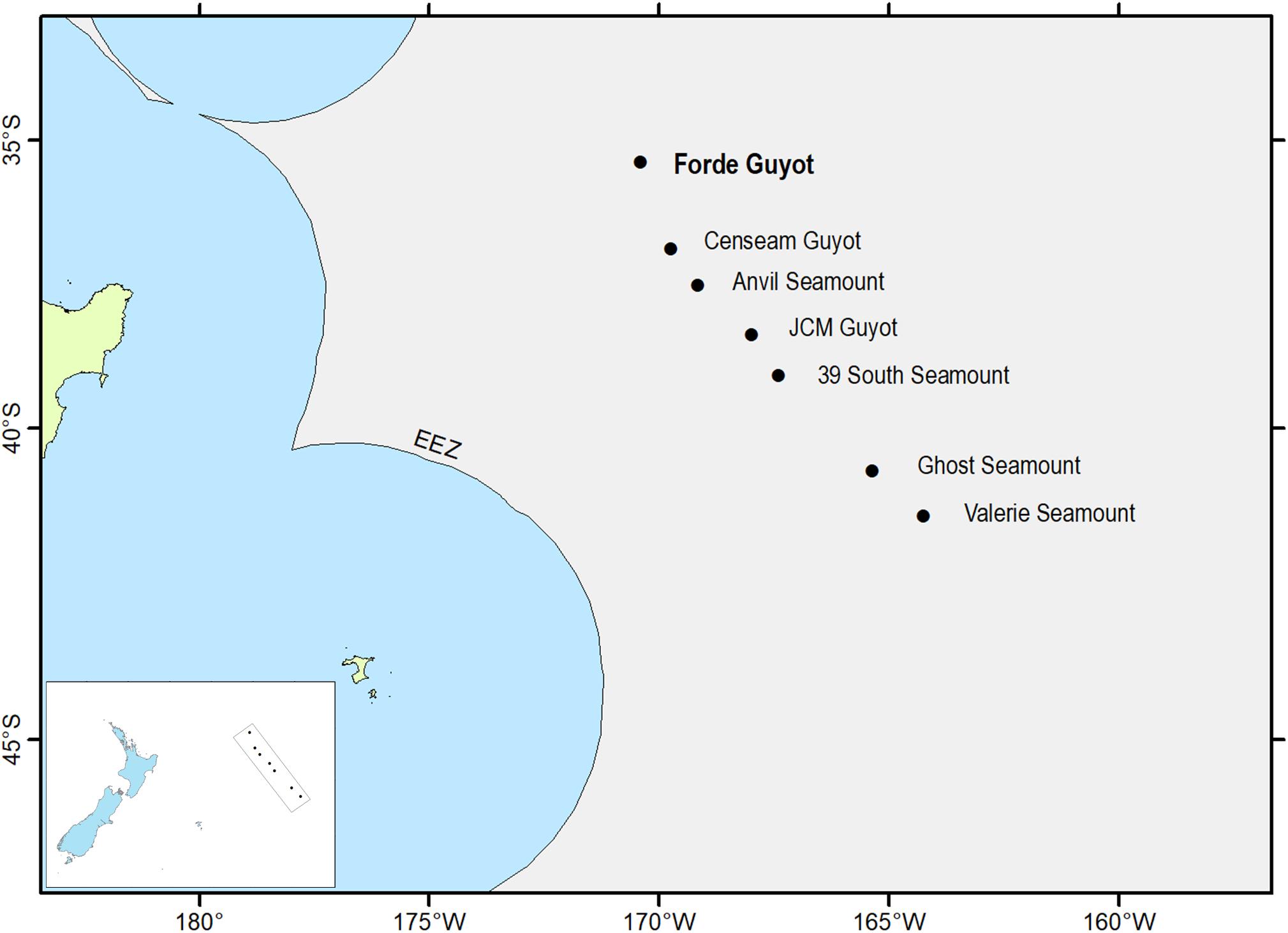
Figure 1. Map showing the summit location of Forde Guyot (bolded feature name) in relation to other seamount features on part of the Louisville Seamount Chain. Inset map shows these seamounts in relation to New Zealand (modified from Rowden et al., 2017).

Data and Data Processing

Video data from Rowden et al. (2017), detailing faunal occurrences and substrate types were reviewed, and nine transects from Forde Guyot in which S. variabilis was present were used in the analysis (Figure 2 and Table 1). For the current study, still images from these transects were also analyzed (Table 1; after review to remove overlapping images, poor quality images, and images taken at >3 m altitude) with S. variabilis and all other visible epifauna (‘morphospecies’ > 10 mm) being counted (using the image annotation platform BIIGLE 2.0; Langenkämper et al., 2017). Because much of the S. variabilis matrix of colonies observed was evidently not alive (dark coloration with no live polyps visible in high resolution still imagery), which is apparently typical for such cold-water coral reef habitat (e.g., Clark and Rowden, 2009; Vertino et al., 2010, and see Figure 3), occurrence of this taxon was recorded in three ways: percent cover of the seabed for live and dead “intact coral” matrix, percent cover of dead broken-up matrix termed “coral rubble,” and counts of distinct live coral colonies or “coral heads” on which live polyps were visible (Figure 3). A coral head was considered distinct if the separation between colonies with live polyps was visually obvious (typically > 5 cm). No minimum or maximum size criteria were used to identify a live coral head, but they were typically in the range of 15–40 cm in diameter.

TABLE 1

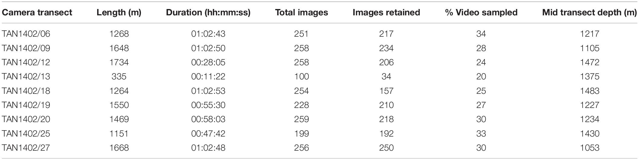
Table 1. Length of each camera transect, video duration, total number of still images taken and retained for analysis, and % of video transect represented by the retained images.

FIGURE 2

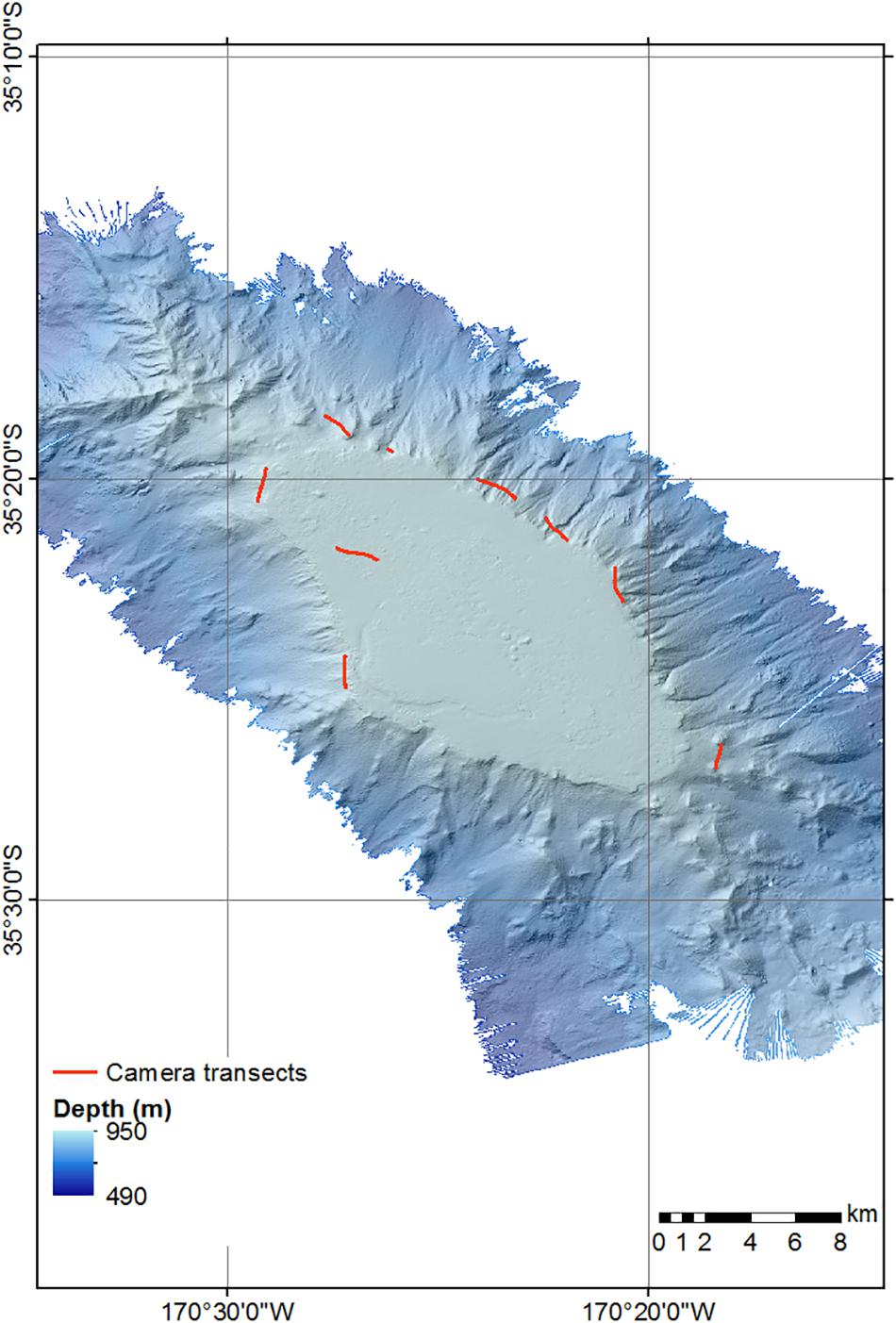
Figure 2. Bathymetric map of Forde Guyot showing the location of the camera transects analyzed for this study.

FIGURE 3

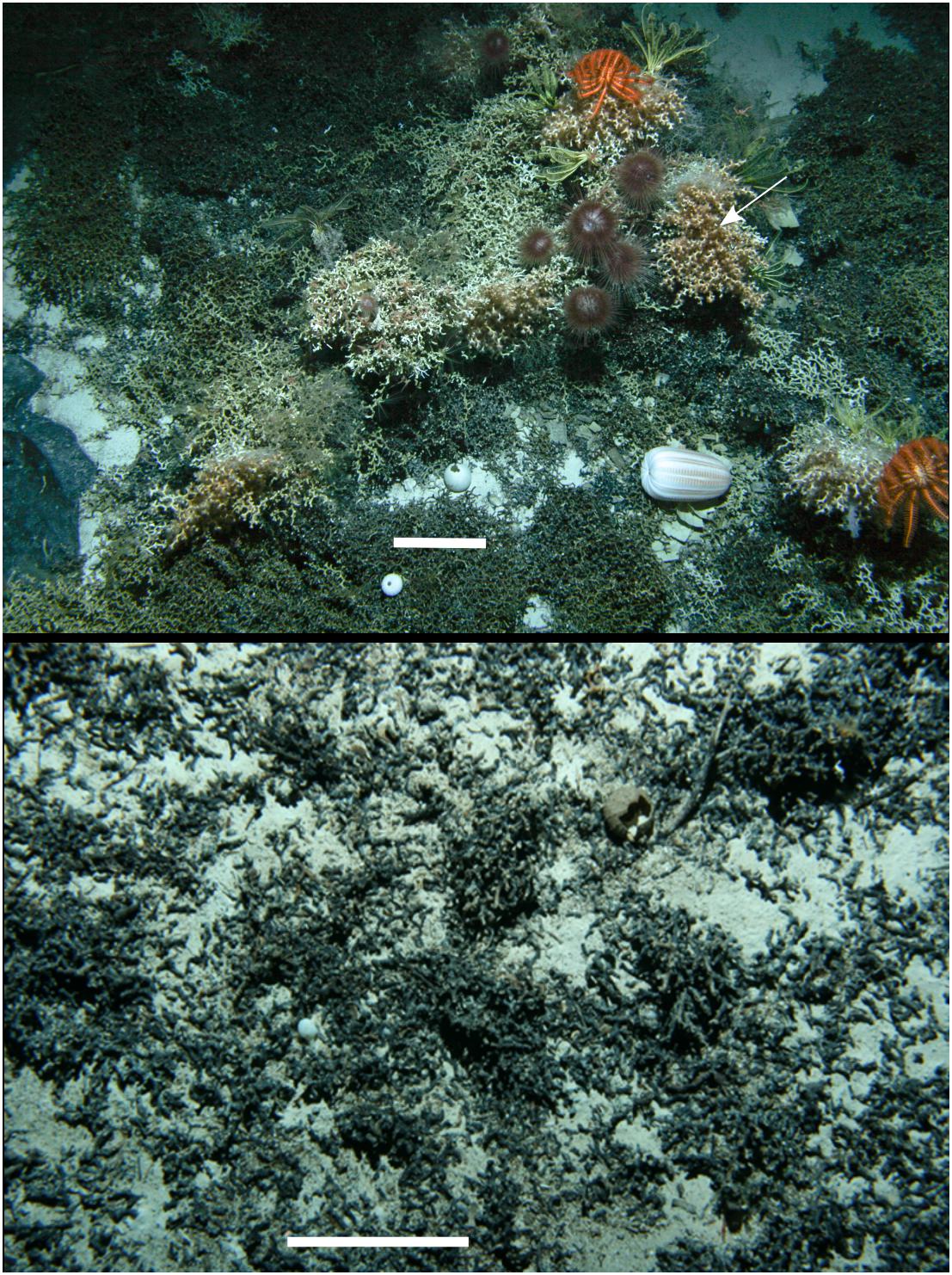
Figure 3. Still images of the seafloor on Forde Guyot showing: (top) intact dead (brown)/live (white and pale orange) coral matrix with live coral heads (distinct pale orange colonies with live polyps; arrow indicates an example of a coral head) of Solenosmilia variabilis, and associated epifauna taxa; (bottom) broken-down dead coral matrix or coral rubble. Scale bar = 20 cm.

Coral and other epifauna records were determined at three spatial scales: per 50 m² segment of video transect (∼2 m transect image width × 24 m along the transect track), per 25 m² segment of video transect (∼2 m transect image width × 12 m along the transect track) and from individual still frames per 2 m² (∼ 2 m × 1 m still image view). Analyses at these spatial scales allow for an examination of whether any identified VME density thresholds were scale dependent, and allow for comparisons with previously published threshold estimates for coral reef habitat.

Data Analysis

Welch’s ANOVA was first used to test if coral habitat (live and dead intact coral and coral rubble) is associated with higher species richness (number of other epifaunal ‘morphospecies’) than non-coral habitat (mainly unconsolidated substrates such as sand and mud). Welch’s ANOVA was used because data had unequal variances.

Data exploration indicated a lack of homogeneity and non-linear relationships within the datasets, which together with the nested structure of the data violate statistical assumptions of methods that fit curves to raw data (Supplementary Figure S1). Thus, general additive models (GAMs) were applied to the datasets to model the relationship between the coral density parameters noted above (predictor variables) and the species richness of other epifauna (response variable). GAMs are generalized models with smoothers and link functions based on an exponential relationship between the response variable and the predictor variables (Zuur et al., 2014b). GAMs have previously been used to model relationships between environmental variables and species richness (Robert et al., 2015; Song and Cao, 2017) and to identify ecological response thresholds (Foley et al., 2015; Large et al., 2015). GAMs were chosen because they can accommodate non-linear relationships and produce ecologically intuitive outputs by identifying the shape and strength of the relationship between the response and predictor variables (Zuur et al., 2014a). Non-linear threshold responses are common in ecological systems, but some non-linear phenomena may not be of direct interest and need to be accounted for when making inferences about the variables in question. Depth and spatial proximity of data points to one another can influence biological responses and were integrated into models via the categorical variable ‘transect.’ To further account for inherent spatial autocorrelation in the data an additional predictor variable, the residual autocovariate (RAC) was calculated and added to the model. The RAC represents the similarity between the residuals from initial models at a location compared with those of neighboring locations. This method can account for spatial autocorrelation without compromising model performance (Crase et al., 2012).

The degree of smoothing in the fitting of the explanatory variables was based on the generalized cross validation (GCV) method and a log link function. For the 2 m² dataset smooth terms allowing up to 4 degrees of freedom were used, due to the low variability in the response values at this resolution. A negative binomial distribution with no transformation was chosen (in part because this provided better fits given the high proportion of zero values) after exploring several alternative distributions (Poisson, quasi-Poisson, zero inflated) and model set ups (different variable explanatory variables and optimized under parsimony). Significance of terms in the model were tested with ANOVA. Model accuracy was assessed by variance in species richness explained by each model (Adjusted R²) and model fit by Akaike’s Information Criterion score (AIC). All statistical analyses were conducted using the open source software R (R Core Team, 2014), packages “mgcv,” “gbm,” “raster” and “vegan.”

Thresholds are characterized by a non-linear change in response to a predictor variable (Foley et al., 2015; Large et al., 2015). Based on ecological theory, we expect the relationship between coral density parameters and associated species richness to exhibit an initial relatively steep positive relationship before flattening off to a plateau or exhibiting a slight drop off as coral density increases. That is, as the amount or density of structurally complex habitat increases so does the number of species that can be supported by this habitat, up until a point where the concentration of habitat has reached a level where all physical niches are occupied by species that have become associated with the habitat (Rosenzweig, 1995, pp. 32–36, and references therein). As the density of the structural habitat increases beyond this threshold, it is possible that the number of associated species may decrease slightly as some species are outcompeted and the number of niches is reduced, assuming an increase in density is associated to some extent with an increase in time (Rosenzweig, 1995, pp. 186–189, and references therein) (Figure 4). Potential coral density thresholds for species richness were identified from the GAMs using four methods: (1) the intersections of linear regressions through the initial and final 5% of the data; (2) the intersection of a linear regression through the initial 5% of data with a horizontal line extended from the maximum cumulative value; (3) the point on a curve fit to the data that is closest to the top-left corner; and (4) the point that maximizes the distance between the curve and a line drawn between the extreme points on the curve (Youden Index) (Supplementary Figure S2). Where possible, all four threshold values were determined for each of the coral density parameters, and the average threshold for each spatial scale calculated.

FIGURE 4

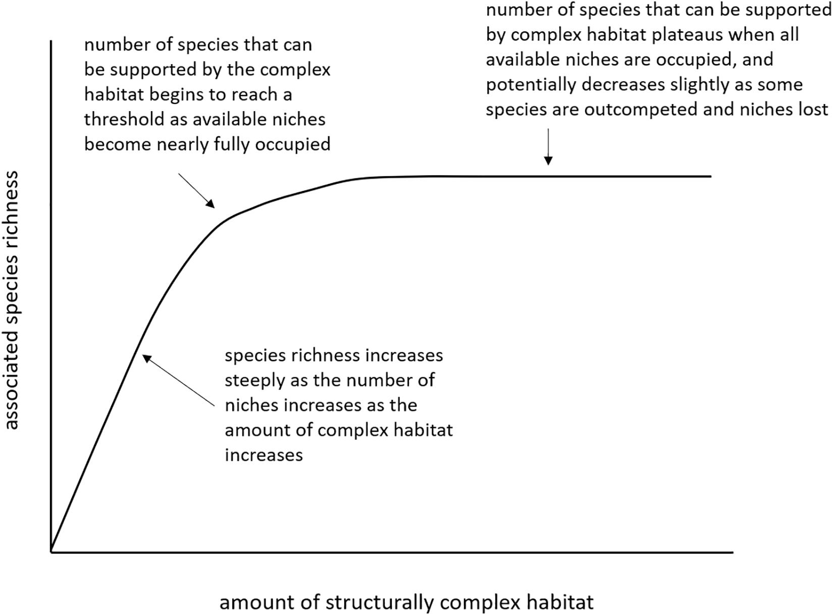
Figure 4. Theoretical relationship between the amount of structurally complex habitat and associated species richness.

Results

See Supplementary Material for species richness data for each spatial scale of the analysis.

One hundred and thirty-six epifaunal morphospecies were identified from the datasets. Epifauna exhibited a patchy distribution, reflected in the species richness counts that were relatively low, and which reached maximum values of 10 at 50 m², 8 at 25 m² and 9 at 2 m². Solenosmilia variabilis also exhibited a patchy distribution occurring at low density across the study transects (Figure 5).

FIGURE 5

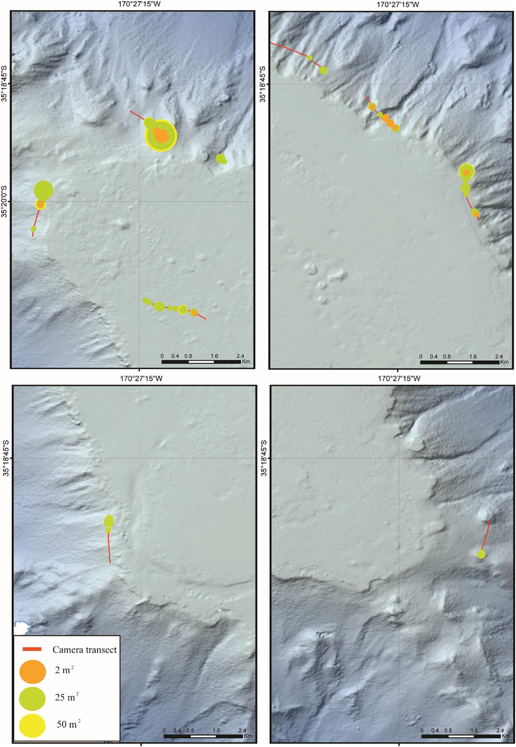
Figure 5. Maps showing the distribution of the abundance of the stony coral Solenosmilia variabilis at three spatial scales (50, 25, and 2 m²). Relative abundance expressed by expanding circles (see key for values). Symbols plotted at the midpoints of the 50 m², 25 m² sections of the camera transects, and at the exact image location for 2 m².

At all spatial scales, average epifaunal species richness was significantly higher for the intact live and dead coral matrix (2.35 50 m^–2, 3.28 25 m^–2, 2.6 2 m^–2), compared to coral rubble (0.98 50 m^–2, 1.56 25 m^–2, 1.09 2 m^–2) and non-coral habitat (0.81 50 m^–2, 1.27 25 m^–2, 1.15 2 m^–2) (Welch’s ANOVA for 50 m² F2, 168 = 61.49, p < 0.001; 25 m² F2, 258 = 77.886, p < 0.001; 2 m² F2, 227 = 20.51, p < 0.001).

The number of live S. variabilis coral heads had the greatest influence on the models for species richness, followed by % cover of intact coral, whilst coral rubble had no significant influence, except at the 50 m² spatial scale. This result is consistent across spatial scales (Table 2).

TABLE 2

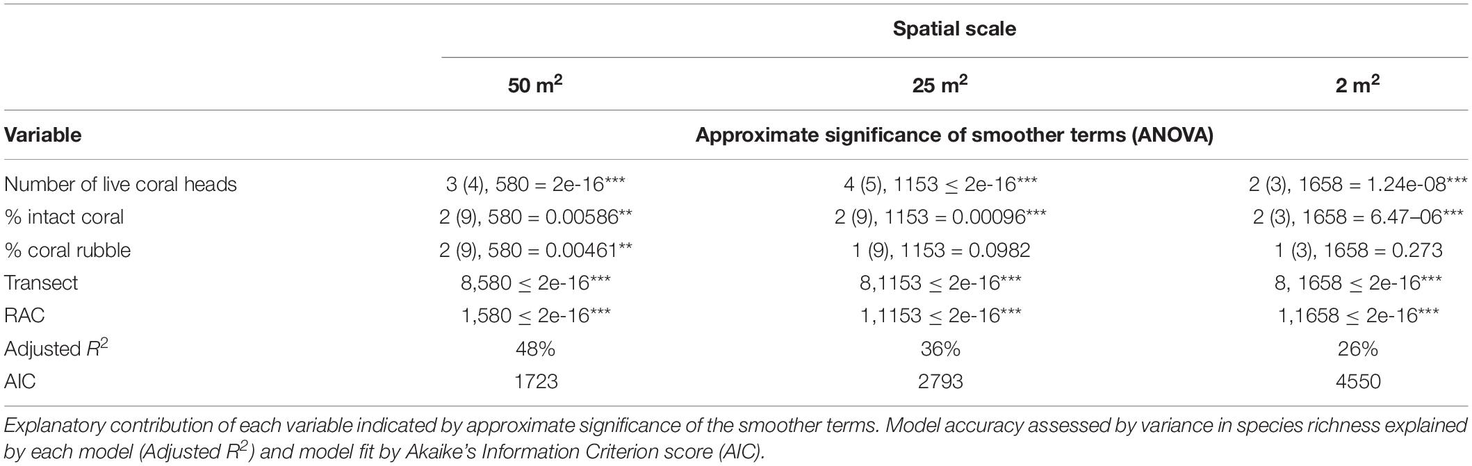
Table 2. Results of the GAM models at three spatial scales.

Species richness exhibited an initial shallow positive response to % intact coral, which flattened or dropped off after reaching thresholds of 26% (50 m²), 24.5% (25 m²) and 28% (2 m²) (Figure 5 and Table 3). The relationships between species richness and % coral rubble were too ‘flat’ to determine thresholds (Figure 6).

TABLE 3

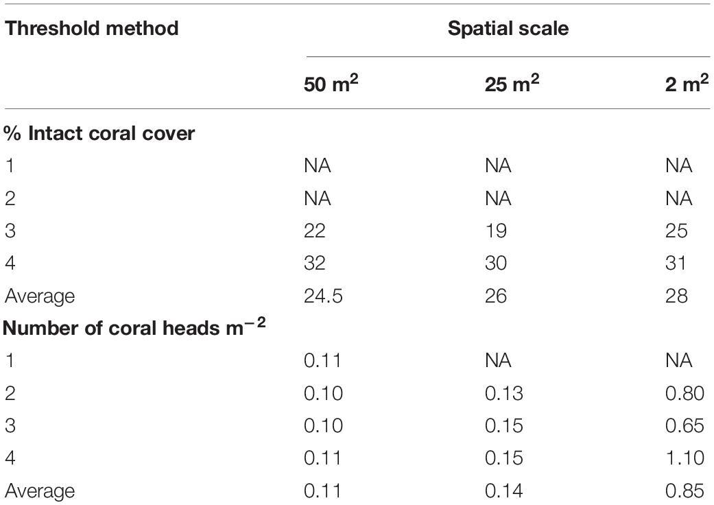
Table 3. Results of the analysis to determine coral density thresholds for identifying structurally complex vulnerable marine ecosystems at three spatial scales (see section Materials and Methods for description of numbered threshold methods).

FIGURE 6

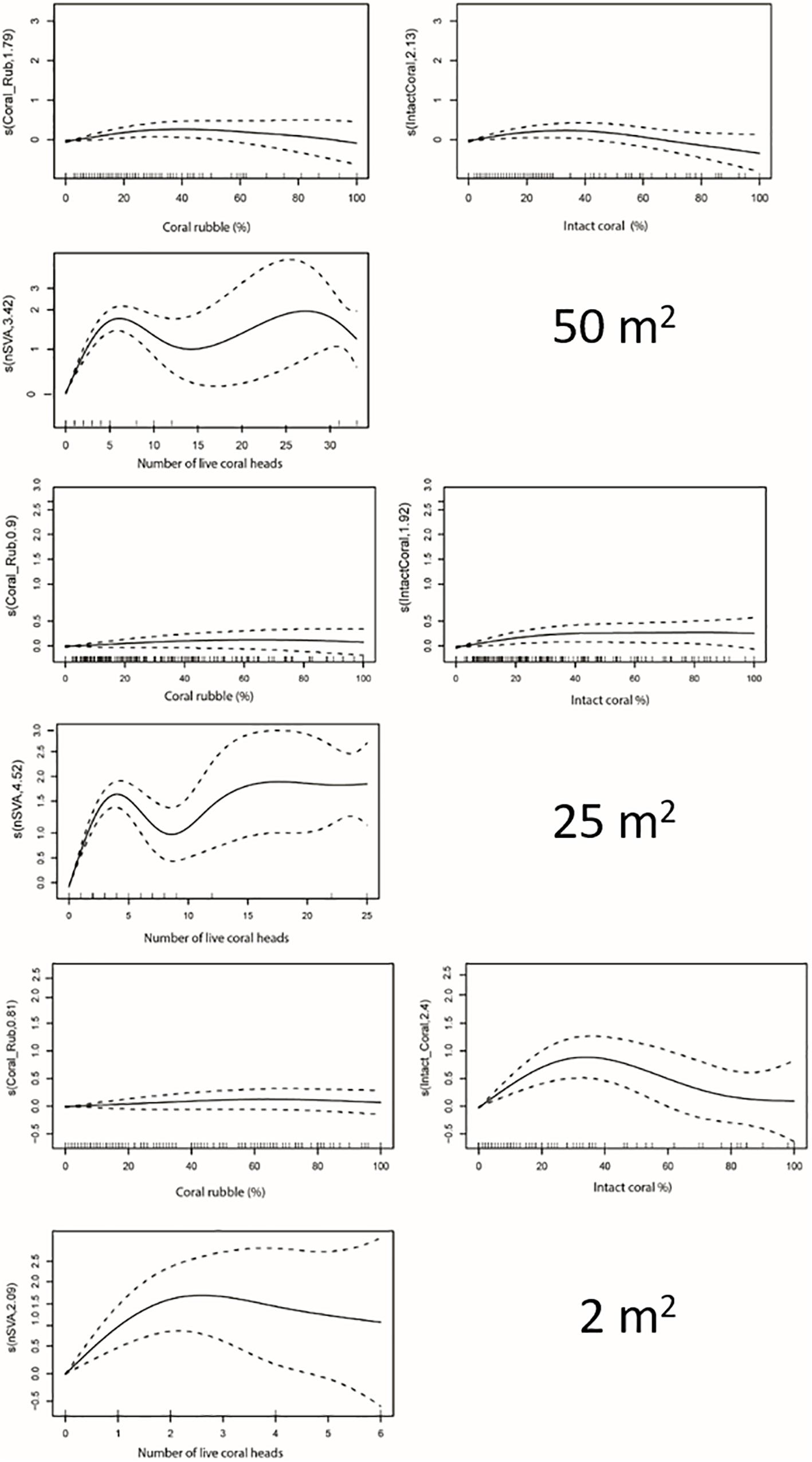
Figure 6. General Additive Model smoother outputs showing the relationship between coral density (% coral rubble, % intact coral, number of live coral heads) and species richness at three spatial scales.

Species richness exhibited an initial steep positive relationship with the number of live coral heads of S. variabilis, before reaching an identifiable threshold beyond which the relationship flattened off in an undulating or slightly decreasing curve (Figure 6). The multimodal response beyond the threshold at the 50 and 25 m² spatial scales appears to reflect inter-transect variability driven by the high density of S. variabilis recorded from one transect (station TAN1402/18) which is responsible for the second maxima. The average density threshold for the number of S. variabilis live heads is similar for both 50 and 25 m² spatial scales of the analysis, when expressed as number of coral heads m^–2; 0.11 and 0.14 m^–2, respectively. The average density threshold for number of live coral heads was 0.85 m^–2 at the 2 m² spatial scale of the analysis (Table 3).

Discussion

We determined density thresholds that can be used to objectively identify structurally complex coral reef VMEs in the SPRFMO Convention Area. We used a methodology that operationalizes one of the criteria for identifying VMEs by determining the “significant concentrations” of a structure forming organism that supports a “high diversity” of associated fauna that are dependent on this structuring organism (FAO, 2009).

Our initial analysis of image data from Forde Guyot on the Louisville Seamount Chain demonstrated that cold-water coral reef habitat formed by the stony coral Solenosmilia variabilis supports elevated levels of biodiversity compared to less structurally complex substrates such as nearby mud and sand. Elevated levels of biodiversity associated with habitat formed by other stony coral species, compared to other deep-sea habitats, have been demonstrated previously in other ocean regions (e.g., Desmophyllum pertusum in the North Atlantic - Henry and Roberts, 2007). However, we are unaware of any published study that has examined the direct relationship between density parameters of cold-water coral reefs and the richness of associated species [but see acknowledgments, and Beazley et al. (2015) and Ashford et al. (2019) for examinations of the density/biomass of other VME indicatar taxa and associated species richness]. A study by Van Den Beld et al. (2017) examined the separate relationships between stony coral cover and the abundance (but not species richness) of solitary coral taxa, and no density threshold for the abundances of these taxa was observed.

Our modeling analysis demonstrated a relationship between coral density and associated species richness at three spatial scales, and identified density thresholds at which coral reef habitat supports relatively higher levels of associated biodiversity. The non-linear relationship conformed to the theoretical expectation on which our study was based (see section Materials and Methods). We acknowledge that a possible alternative explanation, in addition to competition, for any apparent decrease in the number of species associated with coral densities above the thresholds could be related to lower detection probability as habitat-forming taxa become more abundant and increase in complexity. Somewhat surprisingly, the density thresholds for the % cover of the intact coral matrix were similar across all spatial scales (ranging from 24.5 to 28%), as were the thresholds for the number of live coral heads at the 50 m² and 25 m² spatial scales (0.11 and 0.14 m^–2, respectively). The higher coral head density threshold observed for the 2 m² spatial scale (0.85 m^–2) could potentially be explained by a range of factors associated with the two camera systems, including: different observation viewpoints in video and still images; image resolution and lighting differences; and differing spatial scales of observation. The angled viewpoint of the video means that it is possible some coral heads may be obscured by coral matrix in front of them, whereas the vertical viewpoint of the still images will ensure that all live coral heads are observable, thereby resulting in a higher count. The still images are of higher resolution and more evenly lit than the video imagery, which could also result in higher detection rates of the live coral heads in the still images. It is also possible that the identification of thresholds for individual live coral heads are scale-dependent. The cold-water coral reefs were patchy, and because still images sample a smaller seabed area than does video, they are less likely to encounter coral reef patches, which will influence the counts of live coral heads. A further consequence of the smaller seabed area within individual still images (which is typically smaller than the coral patches) is that counts of live coral head density may be higher in still images because larger coral reef patches are more likely to be detected multiple times by the images than smaller habitat patches (assuming larger patches are more dense than smaller patches). Observations made by video at the 50 m² and 25 m² spatial scale will more likely capture whole coral reef patches, and thereby result in more stable and reliable density estimates. Thus, it is clear that scale-related sampling effects should be considered when attempting to determine reliable density estimates of fauna that generate patchy habitats (Andrew and Mapstone, 1987). However, the results for the two larger spatial scales, both derived from the same imaging system, suggest that the relationships and thresholds observed are ecologically fundamental. This finding provides support for the practical application of such objectively identified quantitative thresholds in the identification and mapping of structurally complex VME habitats.

Vertino et al. (2010) subjectively identified 20–40% coverage of live and/or dead coral colonies as a threshold at a spatial scale of 2.4 m² in the Mediterranean Sea. Their result, even though a different species in a different ocean was broadly similar to our objectively derived thresholds of 24.5 – 28% cover. For the one quantitative examination that we know of that examined the relationship between % coral cover and community structure (Price et al., 2019), the derived density threshold is also similar to the one we identify more directly for species richness. Price et al. (2019) found through multivariate analysis that the proportion of live and dead coral cover of stony coral (predominantly Madrepora oculata Linnaeus, 1758 and Desmophyllum pertusum) in the Whittard Canyon (North East Atlantic) was apparently related to community structure, and that coral reef communities become distinct somewhere between a coral cover of 28 and 36% (they suggested 30% as an approximation) at a spatial scale of 10 s of meters. They demonstrated more directly using GAMs that species richness began to plateau at a particular level of structural complexity (0.7 vector ruggedness measure), which they reported (but did not show) as being equivalent to 30% coral cover.

The density thresholds we identified for live coral heads using video data, 0.11 m^–2 and 0.14 m^–2 (at 50 m² and 25 m², respectively), were the same or similar to the threshold of 0.11 m^–2 used previously to identify coral reef VME on the Lousiville Seamount Chain (coverted from 2.78 live heads per 25 m², Rowden et al., 2017). The density threshold used by Rowden et al. (2017) was from the same video data but derived by a different methodology, and based on a subjective definition of what constitutes a coral reef “sensitive environment” according to regulations devised to prevent impacts to such habitats by human activities in the New Zealand EEZ¹. The similarity between the thresholds appears to offer some support for the subjective-based threshold. However, Rowden et al. (2017) urged caution of the use of the threshold they applied, describing it as a subjective regional translation of the “you will know when you see it” descriptions of cold-water coral reefs, and argued for the implementation of quantitative studies such as the present work to objectively identify VMEs. Having now established a quantitative-based threshold to identify VMEs, it is possible to re-map the coral reef habitat on the study seamounts of the Louisville Seamounts Chain. Although the objective and subjective-based thresholds were apparently similar, application of the new density threshold for 25 m² indicates that there is ∼60% less coral reef VME habitat on Forde Guyot than previously estimated (Rowden et al., 2017; 0.12 km² compared to 0.20 km², Figure 7).

FIGURE 7

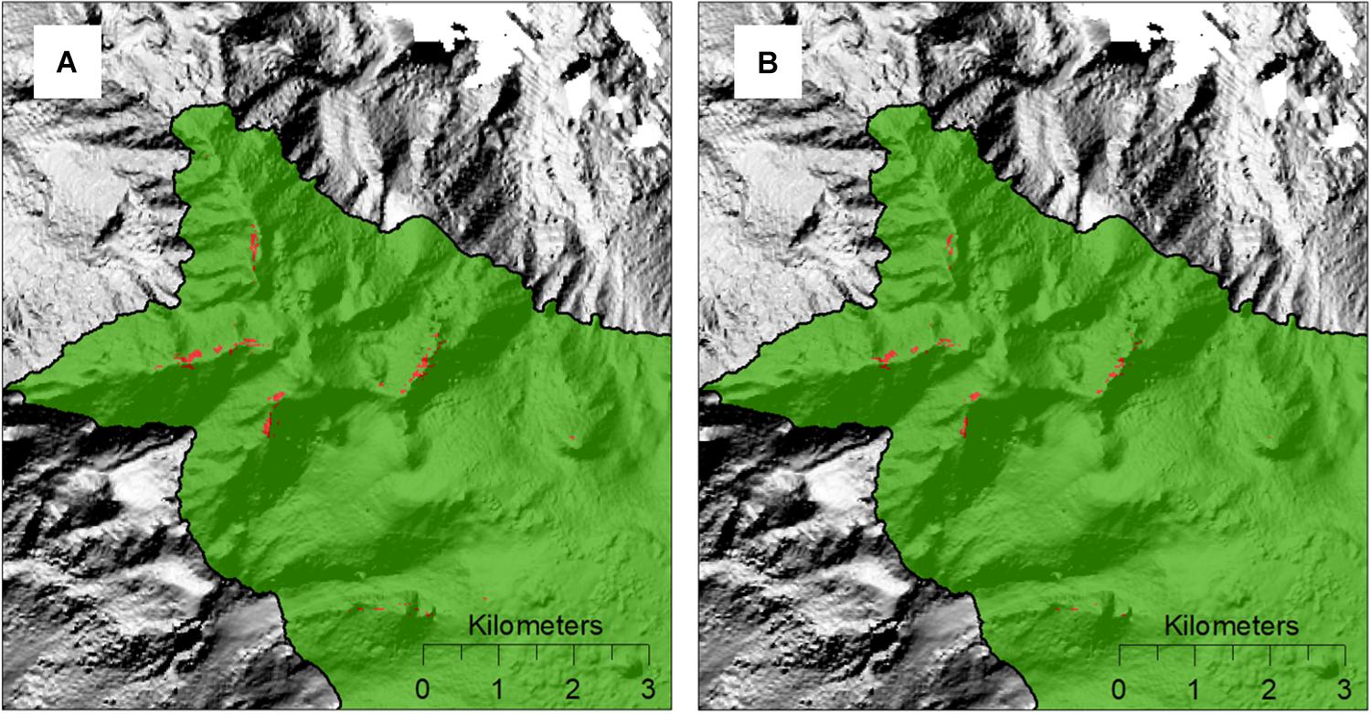
Figure 7. Predicted coral reef VME habitat (red patches) on the north-west portion of Forde Guyot, identified by applying a density threshold for live coral heads to an abundance-based habitat suitability model for Solenosmilia variabilis (Rowden et al., 2017); (A) using the subjectively derived threshold of 2.78 live coral heads 25 m^–2 from Rowden et al. (2017), and (B) the objectively derived threshold of 3.5 live coral heads 25 m^–2 from the present study.

In the present study, low sample size and uneven sampling posed some limitations for modeling the relationship between coral density parameters and associated species richness. However, it appears that low coral density and a patchy distribution is inherent in the nature of the cold-water coral reefs on Forde Guyot, and indeed other seamounts on the Louisville Seamount Chain (Rowden et al., 2017). Future studies should endeavor to better accommodate such heterogeneity in analyses of the relationships that we examined. Despite the potential limitations, we hope our work will encourage future efforts to look further at the taxa/regional-specific or universal nature of the density thresholds determined here for identifying structural complex coral reef VMEs. Quantitative studies establishing the association between coral density parameters and the structural or functional attributes that distinguish VMEs are few, and this lack is currently hindering efforts to devise measures to protect VMEs from the impacts of fishing.

Conclusion

Our data and previous findings suggest that approximately 30% intact coral cover represents a significant concentration which supports a high diversity of associated taxa. This threshold could be used broadly to distinguish deep-sea coral reef VMEs made by structurally complex stony coral species such as Solenosmilia variabilis, Madrepora oculata, and Desmophyllum pertusum. Furthermore, specific threshold density metrics for particular species and regions, such as we derived for number of live coral heads of S. variabilis for the South Pacific, can be used to threshold abundance-based habitat suitability model predictions to make maps that can be used by RFMOs to design spatial management measures to prevent significant adverse impacts to VMEs.

Data Availability Statement

All datasets generated for this study are included in the article/Supplementary Material.

Author Contributions

AR conceived of the study, led the writing, and drafted text for the manuscript. AR, MC, and DB designed the field survey. MC, DB, and OA collected the data from the field survey. TP analyzed the images, conducted the statistical analysis, and contributed draft text to the manuscript. All authors interpreted all data, revised and approved the final version of the manuscript.

Funding

This work was based on data obtained during the NIWA-led South Pacific Vulnerable Marine Ecosystems Project funded by the New Zealand Ministry for Business, Innovation and Employment (C01X1229). AR, DB, OA, and MC’s contribution to the research reported here was funded by NIWA’s Fisheries Centre. TP’s contribution to the research was funded by the Southampton Partnership for Innovative Training of Future Investigators Researching the Environment, which supported her internship at NIWA while a Ph.D. student at the University of Southampton.

Conflict of Interest

The authors declare that the research was conducted in the absence of any commercial or financial relationships that could be construed as a potential conflict of interest.

Acknowledgments

We acknowledge that our study was partly inspired by the poster displayed by Lenaick Menot et al. at the 2018 Deep Sea-Biology Symposium in Monterey, United States (The ecological role of patchy cold-water coral habitats: Does coral density influence local biodiversity in submarine canyons in the Bay of Biscay? http://dsbsoc.org/wp-content/uploads/2014/12/15thDSBS_Abstracts.pdf). We thank Tom Ezard, from the National Oceanography Centre, for his discussions of statistical model validation plots.

Supplementary Material

The Supplementary Material for this article can be found online at: https://www.frontiersin.org/articles/10.3389/fmars.2020.00095/full#supplementary-material

Footnotes

1. ^ http://www.mfe.govt.nz/marine/legislation/regulations-under-eez-act

References

Althaus, F., Williams, A., Schlacher, T. A., Kloser, R. K., Green, M. A., Barker, B. A., et al. (2009). Impacts of bottom trawling on deep-coral ecosystems of seamounts are long-lasting. Mar. Ecol. Progr. Ser. 397, 279–294. doi: 10.3354/meps08248

CrossRef Full Text | Google Scholar

Anderson, O. F., Guinotte, J. M., Rowden, A. A., Clark, M. R., Mormede, S., Davies, A. J., et al. (2016). Field validation of habitat suitability models for vulnerable marine ecosystems in the South Pacific Ocean: implications for the use of broad-scale models in fisheries management. Ocean Coast. Manag. 120, 110–126. doi: 10.1016/j.ocecoaman.2015.11.025

CrossRef Full Text | Google Scholar

Andrew, N. L., and Mapstone, B. D. (1987). Sampling and the description of spatial pattern in marine ecology. Oceanogr. Mar. Biol. 25, 39–90.

Google Scholar

Ashford, O. S., Kenny, A. J., Barrio Froján, C. R. S., Downie, A.-L., Horton, T., and Rogers, A. D. (2019). On the influence of Vulnerable Marine Ecosystem habitats on peracarid crustacean assemblages in the Northwest Atlantic Fisheries Organisation regulatory area. Front. Mar. Sci. 6:401. doi: 10.3389/fmars.2019.00401

CrossRef Full Text | Google Scholar

Beazley, L., Kenchington, E., Yashayaev, I., and Murillo, F. J. (2015). Drivers of epibenthic megafaunal composition in the sponge grounds of the Sackville Spur, northwest Atlantic. Deep Sea Res. Part I Oceanogr. Res. Pap. 98, 102–114. doi: 10.1016/j.dsr.2014.11.016

CrossRef Full Text | Google Scholar

Clark, M. R., Althaus, F., Schlacher, T. A., Williams, A., Bowden, D. A., and Rowden, A. A. (2016). The impacts of deep-sea fisheries on benthic communities: a review. ICES J. Mar. Sci. 73, i51–i69. doi: 10.1371/journal.pone.0022588

PubMed Abstract | CrossRef Full Text | Google Scholar

Clark, M. R., Bowden, D. A., Rowden, A. A., and Stewart, R. (2019). Little evidence of benthic community resilience to bottom trawling on seamounts after 15 Years. Front. Mar. Sci. 6:63. doi: 10.3389/fmars.2019.00063

CrossRef Full Text | Google Scholar

Clark, M. R., and Rowden, A. A. (2009). Effect of deep water trawling on the macro-invertebrate assemblages of seamounts on the Chatham Rise. New Zealand. Deep Sea Res. I 56, 1540–1554. doi: 10.1016/j.dsr.2009.04.015

CrossRef Full Text | Google Scholar

R Core Team, (2014). R: A language and environment for statistical computing. R Foundation for Statistical Computing. Vienna: R Core Team.

Google Scholar

Crase, B., Liedloff, A. C., and Wintle, B. A. (2012). A new method for dealing with residual spatial autocorrelation in species distribution models. Ecography 35, 879–888. doi: 10.1111/j.1600-0587.2011.07138.x

CrossRef Full Text | Google Scholar

Duncan, P. M. (1873). A description of the Madreporaria dredged up during the Expeditions of H.M.S. ‘Porcupine’ in 1869 and 1870. Trans. Zool. Soc. London 8, 303–344.

Google Scholar

FAO, (2009). Management of Deep-Sea Fisheries in the High Seas. Rome: FAO.

Google Scholar

Foley, M. M., Martone, R. G., Fox, M. D., Kappel, C. V., Mease, L. A., Erickson, A. L., et al. (2015). Using ecological thresholds to inform resource management: current options and future possibilities. Front. Mar. Sci. 2:95. doi: 10.3389/fmars.2015.00095

CrossRef Full Text | Google Scholar

Georgian, S. E., Anderson, O. F., and Rowden, A. A. (2019). Ensemble habitat suitability modeling of vulnerable marine ecosystem indicator taxa to inform deep-sea fisheries management in the South Pacific Ocean. Fish. Res. 211, 256–274. doi: 10.1016/j.fishres.2018.11.020

CrossRef Full Text | Google Scholar

Henry, L. A., and Roberts, J. M. (2007). Biodiversity and ecological composition of macrobenthos on cold-water coral mounds and adjacent off mound habitat in the bathyal Porcupine Seabight. Ne Atlantic. Deep Sea Res I 54, 654–672. doi: 10.1016/j.dsr.2007.01.005

CrossRef Full Text | Google Scholar

Hill, P. (2009). Designing a deep-towed camera vehicle using single conductor cable. Sea Technol. 50, 49–51.

Google Scholar

Howell, K. L., Holt, R., Endrino, I. P., and Stewart, H. (2011). When the species is also a habitat: comparing the predictively modelled distributions of Lophelia pertusa and the reef habitat it forms. Biol. Conservat. 144, 2656–2665. doi: 10.1016/j.biocon.2011.07.025

CrossRef Full Text | Google Scholar

Koslow, J. A., Gowlett-Holmes, K., Lowry, J. K., O’hara, T., Poore, G. C. B., and Williams, A. (2001). Seamount benthic macrofauna off southern Tasmania: community structure and impacts of trawling. Mar. Ecol. Progr. Ser. 213, 111–125. doi: 10.3354/meps213111

CrossRef Full Text | Google Scholar

Langenkämper, D., Zurowietz, M., Schoening, T., and Nattkemper, T. W. (2017). BIIGLE 2.0 - Browsing and annotating large marine image collections. Front. Mar. Sci. 4:83. doi: 10.3389/fmars.2017.00083

CrossRef Full Text | Google Scholar

Large, S. I., Fay, G., Friedland, K. D., and Link, J. S. (2015). Critical points in ecosystem responses to fishing and environmental pressures. Mar. Ecol. Progr. Ser. 521, 1–17. doi: 10.3354/meps11165

CrossRef Full Text | Google Scholar

Linnaeus, C. (1758). Systema Naturae Per Regna Tria Naturae, Secundum Classes, Ordines, Genera, Species, Cum Characteribus, Differentiis, Synonymis, Locis, 10th Edn, Vol. 1., Holmiae: Laurentius Salvius, 824. doi: 10.5962/bhl.title.542

CrossRef Full Text | Google Scholar

Parker, S. J., Penney, A. J., and Clark, M. R. (2009). Detection criteria for managing trawl impacts to Vulnerable Marine Ecosystems in high seas fisheries of the South Pacific Ocean. Mar. Ecol. Progr. Ser. 397, 309–317. doi: 10.3354/meps08115

CrossRef Full Text | Google Scholar

Price, D. M., Robert, K., Callaway, A., Lo Lacono, C., Hall, R. A., and Huvenne, V. A. I. (2019). Using 3D photogrammetry from ROV video to quantify cold-water coral reef structural complexity and investigate its influence on biodiversity and community assemblage. Coral Reefs 38, 1007–1021. doi: 10.1007/s00338-019-01827-3

CrossRef Full Text | Google Scholar

Robert, K., Jones, D. O. B., Tyler, P. A., Van Rooij, D., and Huvenne, V. A. I. (2015). Finding the hotspots within a biodiversity hotspot: fine-scale biological predictions within a submarine canyon using high-resolution acoustic mapping techniques. Mar. Ecol. 36, 1256–1276. doi: 10.1111/maec.12228

CrossRef Full Text | Google Scholar

Rosenzweig, M. L. (1995). Species diversity in space and time. Cambridge: Cambridge University Press.

Google Scholar

Rowden, A. A., Anderson, O. F., Georgian, S. E., Bowden, D. A., Clark, M. R., Pallentin, A., et al. (2017). High-resolution habitat suitability models for the conservation and management of vulnerable marine ecosystems on the Louisville Seamount Chain, South Pacific Ocean. Front. Mar. Sci. 4:335. doi: 10.3389/fmars.2017.00335

CrossRef Full Text | Google Scholar

Song, C., and Cao, M. (2017). Relationships between plant species richness and terrain in middle sub-tropical eastern China. Forests 8:344. doi: 10.3390/f8090344

CrossRef Full Text | Google Scholar

UNGA, (2006). United Nations General Assembly. Sustainable fisheries, including through the 1995 agreement for the implementation of the provisions of the United Nations convention on the law of the sea of 10 December 1982 relating to the conservation and management of straddling fish stocks and highly migratory fish stocks, and related instruments. New York: UNGA.

Google Scholar

UNGA, (2009). United Nations General Assembly. Sustainable fisheries, including through the 1995 agreement for the implementation of the provisions of the United Nations convention on the law of the sea of 10 December 1982 relating to the conservation and management of straddling fish stocks and highly migratory fish stocks, and related instruments. General Assembly Resolution 64/72, 2009; A/RES/64/72. New Yorl: UNGA.

Google Scholar

Van Den Beld, I. M. J., Bourillet, J.-F., Arnaud-Haond, S., De Chambure, L., Davies, J. S., Guillaumont, B., et al. (2017). Cold-water coral habitats in submarine canyons of the Bay of Biscay. Front. Mar. Sci. 4, 1–30. doi: 10.3389/fmars.2017.00118

CrossRef Full Text | Google Scholar

Vertino, A., Savini, A., Rosso, A., Di Geronimo, I., Mastrototaro, F., Sanfilippo, R., et al. (2010). Benthic habitat characterization and distribution from two representative sites of the deep-water SML Coral Province (Mediterranean). Deep Sea Res. Part II Top. Stud. Oceanogr. 57, 380–396. doi: 10.1016/j.dsr2.2009.08.023

CrossRef Full Text | Google Scholar

Williams, A., Schlacher, T. A., Rowden, A. A., Althaus, F., Clark, M. R., Bowden, D. A., et al. (2010). Seamount megabenthic assemblages fail to recover from trawling impacts. Mar. Ecol. 31, 183–199. doi: 10.1111/j.1439-0485.2010.00385.x

CrossRef Full Text | Google Scholar

Zuur, A., Ieno, E., Walker, N., Saveliev, A., and Smith, G. (2014a). Mixed effects models and extensions in ecology with R. Berlin: Springer.

Google Scholar

Zuur, A., Saveliev, A., and Ien, E. (2014b). A beginner’s Guide to Generalised Additive Mixed Models with R. United Kingdom: Kingdom.

Google Scholar