Effects of the Temporal Variability of Storm Surges on Coastal Flooding

Introduction

Coastal flooding due to extreme water levels constitutes a major hazard for coastal systems and low-lying areas (Vousdoukas et al., 2018). Such flooding events are likely to become more frequent under sea-level rise on global and local scales, which contributes to an expected increase in the intensity and probability of extreme water levels over the next decades (Church et al., 2013; Arns et al., 2017; Wahl et al., 2017; IPCC, 2019). Furthermore, coastal zones are heavily populated areas which attract many people and are therefore characterized by higher rates of population growth and urbanization in comparison to landlocked regions (Wong et al., 2014; Neumann et al., 2015). This results in an increased exposure of people and assets to coastal flooding. Managing coastal flood risk is a crucial aspect of adapting to these challenging developments, and is becoming increasingly important for coastal communities (Wadey et al., 2015; Vousdoukas et al., 2016). To obtain sustainable adaptation solutions, coastal management strategies must take climate change, socio-economic development and urbanization into account.

Analyzing coastal flood risk requires quantifying damages associated with specific return water levels (Stewart and Melchers, 1997). This is commonly done by means of inundation modeling. However, a number of uncertainties arise during this process, and it is important that they are quantified and communicated to policy-makers (Teng et al., 2017). First, uncertainties arise as a result of the methods used to model inundation, the specific model used and the model parameters (Wahl et al., 2017). A number of different model types and methods are available for use in flood risk assessments, depending on factors such as scale, investigation focus, application purpose, data availability, computing capacity, location characteristics, and others. 2D-hydrodynamic models, which simulate water propagation according to certain physical properties, have gained much attention in recent years (Néelz and Pender, 2013). These models are able to simulate water velocity, flood extent and inundation depth with high accuracy, which is an important requirement for flood risk assessment and management. However, due to their high data and computational requirements, they are mostly applied at local scales. For large-scale applications simplified conceptual models can be used, which calculate inundation based on simplified hydraulic concepts (Teng et al., 2017). These approaches, such as the bathtub method or simple hydrodynamic models, are less accurate than 2D-hydrodynamic models but require far less resources for computation. A comparison of different types of models that are applicable on a large scale can be found in Vousdoukas et al. (2016).

A second source of uncertainty is the estimation of return water levels, which is affected by the length of available water level records. These records are often limited to a few decades and may not contain events of exceptional magnitude. Consequently, return water levels can be significantly underestimated (Dangendorf et al., 2016). In addition, flood risk analyses typically only consider the peak water level of extreme events, and do not consider the effect of other storm surge parameters, such as duration or variability (Wahl et al., 2017). In particular, the temporal variability of extreme sea level events can result in large uncertainties in the estimation of flood impact (Quinn et al., 2014; Santamaria-Aguilar et al., 2017). Despite the ability of hydrodynamic models to account for water propagation and inundation during a complete storm surge curve, temporal variability typically is disregarded in flood risk analyses (Gallien et al., 2014). Such models are commonly forced by water level time-series of past extreme events, or an upscaling of such events to specific return water levels (Santamaria-Aguilar et al., 2017). Therefore, the modeled inundation is only representative for a specific event. Care must be taken as disregarding uncertainties arising from estimates of extreme water levels, storm surge variability and model application can lead to inadequate coastal risk management (Quinn et al., 2014; Santamaria-Aguilar et al., 2017). Therefore, a variety of possible extreme water levels with temporal developments typical for the investigated area are required to account for the range of uncertainties and to produce a more accurate risk assessment. One approach to generate a sufficient number of extreme water level events is outlined in Wahl et al. (2011), who developed a method to stochastically simulate large numbers of extreme water level curves at two locations in the North Sea, Cuxhaven and Hörnum, based on observed events. This approach is further developed by MacPherson et al. (2019) and applied along the micro-tidal German Baltic Sea coast, generating artificial events at 45 tide gauge stations. The model contains three methodological main steps; identification of extreme events within water level records, parameterization of each identified event, and the generation of artificial events using Monte-Carlo Simulations.

This study assesses the influence of the temporal variability of storm surges on flood characteristics in coastal zones for the case of the city of Eckernförde. For this analysis, five statistically simulated storm surge events generated by MacPherson et al. (2019) are simulated using the hydrodynamic model Delft3D (Deltares, 2018). To analyze variations in flood extent and inundation depth due to temporal variability, each event has the same peak water level corresponding to a univariate return period of 200 years but with varying durations and intensities, which we chose artificially to the specified return period. Intensity is hereby defined as the area between the water level curve and a pre-defined threshold, in this case, mean sea-level. Additionally, we consider one sea-level rise projection to examine the effect of higher mean water levels on deviations in both flood characteristics and exposure due to storm surge temporal variability. The paper is structured as follows: the characteristics of the study area as well as the model and the data used for the analysis are described in section “Study Area and Data”; the applied model setup and the generation of the simulated scenarios are outlined in section “Materials and Methods”. The results of the study are presented in section “Results” and discussed in section “Discussion”. Last, the most important findings are provided as concluding statements in section “Conclusion”.

Study Area and Data

Study Area

Eckernförde Bay is located in the south-west Baltic Sea in Kiel Bay and has a length of approximately 16 km (Figure 1). The shallow, elongated bay was formed during the last glacial period (Hofstede, 2008). Its topography is mostly characterized by a gradual coast and low-lying coastal areas with elevation below 10 m referenced to the vertical datum DHHN92 and a maximum elevation of approximately 50 m in the hinterland. The south-eastern coastline of the bay consists of cliffs. The tidal range in the Baltic Sea is small (less than 10 cm) and major variations in water levels are mostly defined by large scale atmospheric pressure and wind (Gräwe and Burchard, 2012). Extreme water levels are mainly influenced by strong north-easterly winds, but seiches acting over the entire Baltic Sea may contribute several decimeters as well (Jensen and Müller-Navarra, 2008). The municipality of Eckernförde has experienced several extreme flood events in the past. The highest event recorded reached 3.15 m above mean sea-level during the 1872 storm surge (WSA Lübeck, 2017), approximately 1 m higher than all following events. The storm surge resulted in 271 fatalities and represents the beginning of systematic planning of flood defenses and protection measures at the Baltic Sea coast in Schleswig-Holstein (Hofstede, 2008).

FIGURE 1

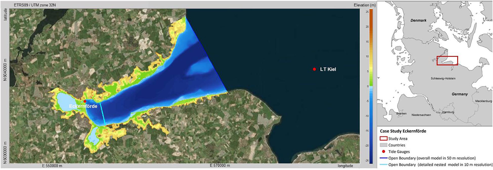
Figure 1. Location of the study area Eckernförde Bay and computational domain of the nested model setup in Delft3D including the tide gauges and the open boundaries of the coarser and the nested model. Bathymetry is displayed in shades of blue and land surface is displayed in green to red colors. The coastal boundary runs along NHN.

The city of Eckernförde has a population of 22,031 inhabitants (status 30.09.2017, City of Eckernförde) and is situated at the western tip of Eckernförde bay in Schleswig-Holstein, the northernmost federal state of Germany. As a Baltic Seaside resort, it is a popular tourist location in the region. Although there is a certain level of coastal defense measures, such as dikes along the federal road or bulkheads, and the area is protected against moderate storm surges, parts of the city are vulnerable to low-frequency, high-magnitude events (PROKOM GmbH, 2017). This is especially true for the city center where economic activities and population are concentrated and elevation is low (large areas beneath 5 m elevation). Martinez and Bray (2011) analyzed the awareness of political decision-makers regarding climate change and possible adaptation in the German Baltic Sea region. Although there is certain recognition of climate change and sea-level rise, knowledge is lacking on how to use the information for appropriate adaptation responses.

Flood risk assessments in Schleswig-Holstein are conducted by simulating flood events using site-specific water levels. As safety standards for coastal protection measures, the federal state uses water levels with a 200-year return period and adds 0.5 m to account for sea-level rise (Ministerium für Energiewende, Landwirtschaft, Umwelt und ländliche Räume des Landes Schleswig-Holstein, 2012). However, the temporal evolution of storm surge events, namely differences in storm surge intensity and duration, are not considered and methods to account for this aspect are not described. On behalf of the city administration of Eckernförde, a master plan to develop an integrated coastal zone management program was published in 2017 (PROKOM GmbH). This plan includes strategies for protecting the coast of the Eckernförde Bay against future floods, and suggests flood protection walls as the main strategy of protection.

Data

Data preparation and processing for the hydrodynamic simulation was performed in ArcGIS (10.3.1), Delft Dashboard, R-Studio (1.1.423), and Matlab (R2016b). The following datasets are used as a basis for the model setup and further analysis (Table 1).

TABLE 1

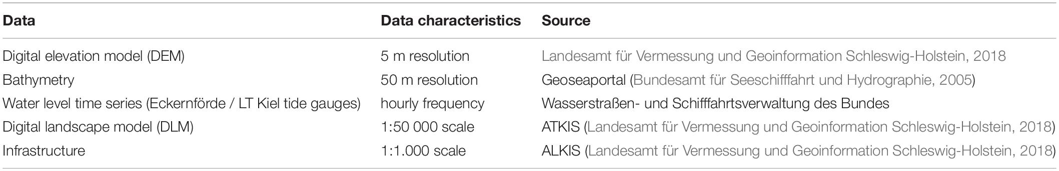
Table 1. Summary of data.

Water level data were used for model boundary forcing and for the calibration and validation of the model setup. We use data measured at two tide gauges (TG) located in the area of Eckernförde Bay, TG Eckernförde which is located in the harbor of Eckernförde, and TG LT Kiel, located approximately ten kilometers to the east (Figure 1). Water level time series for both tide gauges was provided by “Wasserstraßen- und Schifffahrtsamt Lübeck” (WSA Lübeck) department of “Wasserstraßen- und Schifffahrtsverwaltung des Bundes” (WSV). The hourly records cover a time period of 27 years from the 1st November 1990 until the 31st October 2017. Furthermore, the Digital Landscape Model (DLM) is used to structure the study area according to different land uses and land covers. We prepared a bottom roughness map with spatially varying Manning’s roughness coefficients as the landscape characteristics of the floodplain are important for the water propagation.

For the final simulations we use five events of the artificial events stochastically generated by MacPherson et al. (2019) which are based on the LT Kiel and Eckernförde tide gauge records. Here, extreme events are identified within the tide-gauge records and characterized according to a number of specific parameters, such as peak water level, event duration, storm surge shape, etc. By modeling parameter dependencies using a Gaussian copula, a large number of artificial events may be generated through Monte-Carlo Simulations, each as a time series of water levels referred to as hydrographs. From the tide gauge record of LT Kiel, no event corresponding to a return period of 200 years is present. However, using the stochastic model developed by MacPherson et al. (2019), several such events are generated. We selected five events for our study, with peak water levels corresponding to a 200 year return period and a range of intensities.

Materials and Methods

Hydrodynamic Model

Hydrodynamic models are a common tool used in simulating detailed flood dynamics. In this study, we use Delft3D-FLOW, a module of the Delft3D computational program created to simulate processes related to flow, sediment transport, waves, water quality, etc. for coastal, river and estuarine areas (Deltares, 2014). The FLOW module is a complex, multi-dimensional hydrodynamic model which can be used for 3D-simulations or 2D-simulations (depth averaged) where flow and transport phenomena are solved using the unsteady shallow water equation. In this analysis, we use a 2D-model to calculate flow on a Cartesian rectilinear grid.

Model Setup, Calibration and Validation

A rectilinear model grid of Eckernförde Bay (approx. 119.63 km²) was constructed with a resolution of 50 m (Figure 1). This model is forced with water levels at the open boundary using data from the tide gauge LT Kiel. For a more accurate representation of inundation in the city of Eckernförde, we constructed a second nested model grid of the western bay area (approx. 20 km²) with a resolution of 10 m. This nested model is forced with parameters extracted from the coarser model. Running one high resolution model over the whole domain is not feasible due to computational restrictions. Modeled water levels are recorded in 3 min intervals at select locations, most importantly at the location of the tide gauge Eckernförde (see blue lines in Figure 2) which is used for model calibration. Simulations run for periods of 34–100 h depending on the simulated event. Computational time steps are defined based on the CFL number. This results in a time step (at which stability is still given) of 18 s for the overall model and 1.8 s for the detailed model. The focus of this study is the area covered by the nested model, where the city of Eckernförde is located. Therefore, the output of the coarse model is not further analyzed, and is used only for boundary forcing of the high-resolution nested model.

FIGURE 2

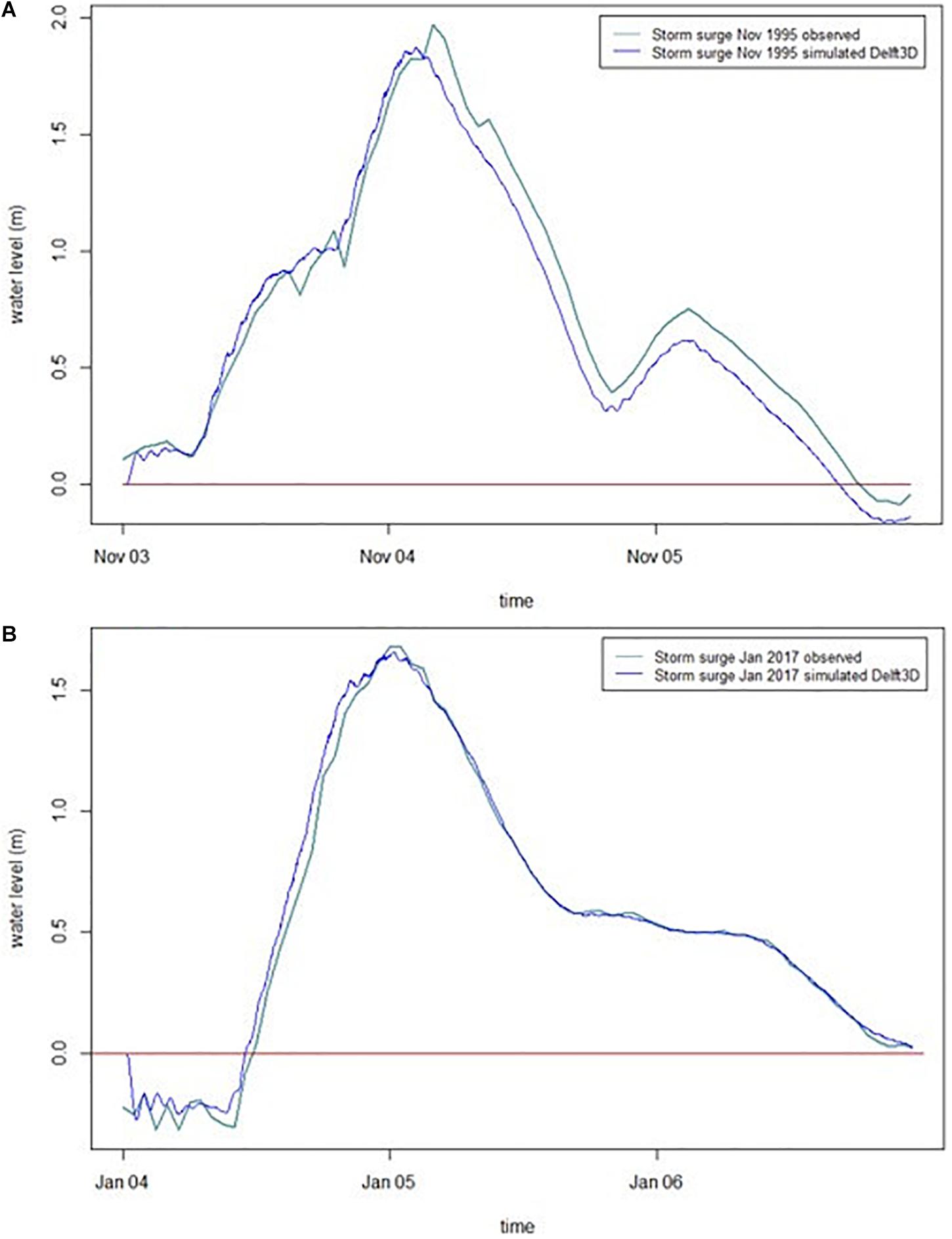
Figure 2. Comparison of observed and simulated water levels November 1995 (A) and January 2017 (B) at the tide gauge Eckernförde.

We calibrate the model using two observed storm surge events which occurred in November 1995 and January 2017. To determine the performance of the model, modeled water levels at TG Eckernförde were compared to observations using root mean square error (RMSE) and model skill (Willmott, 1984). The calibrated model performs well with a RMSE of 0.117 m and 0.061 m, and model skill of 0.988 and 0.998 for the 1995 and 2017 events, respectively. Here, a model skill of 1 would suggest perfect correlation and 0 no correlation. The model slightly underestimates the peak water level by 10 cm, most likely due to the lack of atmospheric forcing (Figures 2A,B). Atmospheric forcing is not considered as the final simulations will be based on artificial water levels, where no observed/simulated atmospheric data exists. Overall, the model simulates water levels with high accuracy and we therefore consider the setup of the model to be suitable for the study area.

Validation of flood extent and depth is challenging due to a lack of observations. There exists no record or exact documentation of these parameters, for example via pictures (on social media) or remote sensing. Nevertheless, a comparison of several newspaper articles on the January 2017 event allows for the calculation of flood extent. Here, the storm surge reached a maximum water level of 1.625 m above NHN (WSA Lübeck). This led to a filling of the harbor basin at the end of the bay and to minimal overtopping. Based on newspaper articles, there were two critical points at both sides of the harbor where the quay wall was overtopped. However, personnel responsible for the emergency action protected buildings with sandbags so that damages were avoided and buildings were not affected (Kühl, 2017; Rohde, 2017; Technisches Hilfswerk Ortsverband Eckernförde, 2017). We compare modeled flood extent with that estimated using the descriptions and photos in the newspaper articles as a method to validate the model. Here, we see basic agreement between the exposed buildings named in the articles (e.g., “Hotel/Restaurant Siegfried-Werft” and “Yachtsport-Geschäft Nielsen”) and those buildings which intersect the modeled flood extent (Figure 3).

FIGURE 3

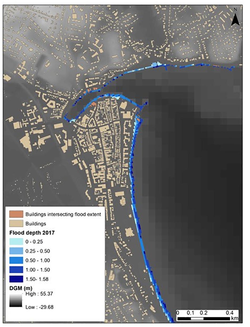
Figure 3. Simulated flood extent for the January 2017 storm surge.

Land Use Classification and Manning’s Roughness Coefficients

The propagation of water in the model is highly influenced by the characteristics of the Digital Elevation Model (DEM) and the roughness of the surface. Surface roughness, induced for example by the presence of vegetation, causes flow resistance and leads to reduced current velocities (Mignot et al., 2006). A common approach in estimating the bottom friction within flood simulations is the attribution of specific coefficients to land use types and land cover. One of the most widely used coefficients for flow computation is the Manning’s roughness coefficient (Garzon and Ferreira, 2016). Therefore, a map with spatially varying Manning’s roughness coefficients according to land use classes is included in the simulation. Common Manning values are obtained from published literature (Fisher and Dawson, 2003; Phillips and Tadayon, 2006; Hossain et al., 2009; Oregon Department of Transportation, 2014; Garzon and Ferreira, 2016). We performed five model runs in order to investigate the sensitivity of the model to changes in the roughness parameter using the five parameterizations described in the following paragraph (Table 2).

TABLE 2

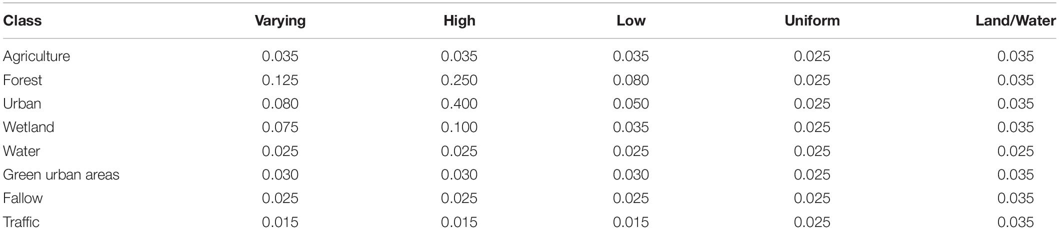
Table 2. Manning’s roughness coefficients for land use classes.

The land use classification in this analysis is based on ATKIS data categories, which are grouped into classes (Table 2). The second column shows a mean value of the Manning coefficients found in the reviewed literature for every land use class. Since the range of the recommended values for some classes (forest, urban, wetland) is large, additional simulations with the lowest and highest value (Table 2 column 3 and 4) for these classes are performed. Some studies also use a uniform value representative for the whole study area or only differentiate between land and water areas (Quinn et al., 2014; Garzon and Ferreira, 2016). Therefore, two additional setups are tested. The first setup consist of a uniform roughness value (0.025) for the entire model domain, while the second uses a uniform value (0.035) for all land surface areas combined with a separate value (0.025) for water surfaces.

Model Simulations

To test the effect of temporal variability on flood extent, the model is forced using water levels from extreme sea-level hydrographs generated stochastically. The temporal variability of the storm surge is described by the storm surge intensity. Five hydrographs of the stochastically simulated events from MacPherson et al. (2019) at the tide gauge LT Kiel are used as boundary conditions in the hydrodynamic simulations (Figure 4). Each storm surge event reaches a peak water level which is equally probable (return period of 200 years: 1.98 m), but with varying durations and intensities (see Table 3 and Figure 4). Waves are not considered in this study as we focus on the effect of storm-surge temporal variability on inundation.

FIGURE 4

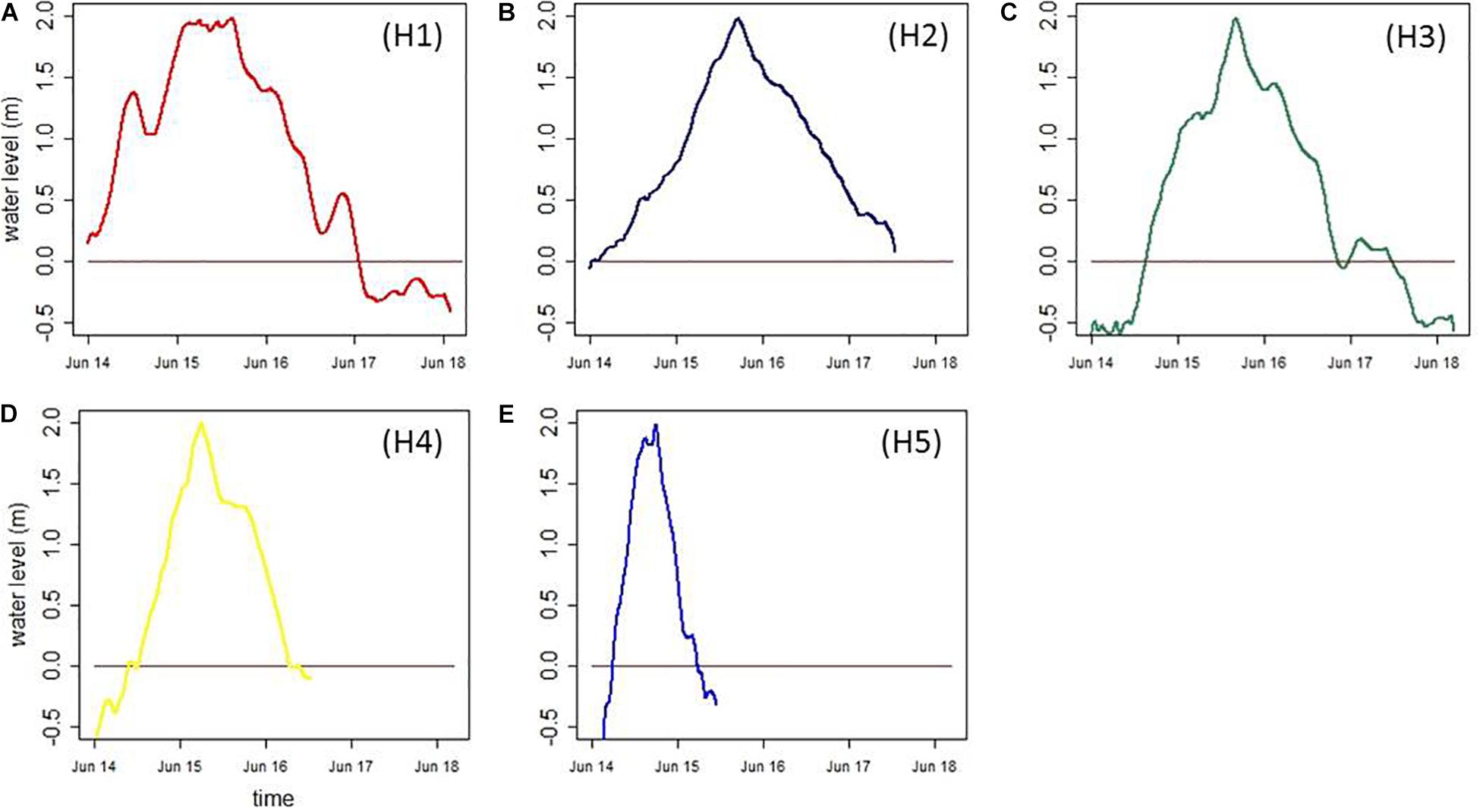
Figure 4. Five selected hydrographs [H1 (A), H2 (B), H3 (C), H4 (D), and H5 (E)] of the simulated storm surge events by MacPherson et al. (2019) for the tide gauge LT Kiel.

TABLE 3

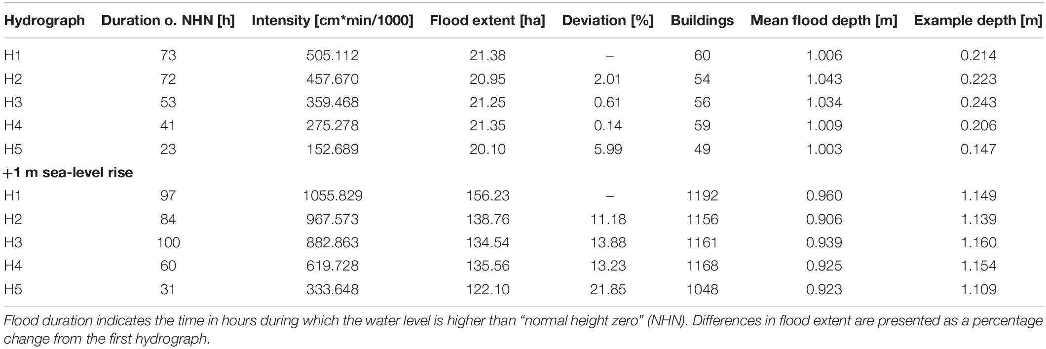
Table 3. Results for all five hydrographs with water levels corresponding to a 200-year return period and in combination with 1 m sea-level rise.

We also consider a number of simulations where future sea level rise is accounted for by manually adjusting the heights of the artificial hydrographs. However, there is high uncertainty regarding the development and dimension of future sea-level rise (Vermeersen et al., 2018). Hinkel et al. (2014) employed a median global mean sea-level rise of 74 cm for RCP 8.5 (Representative Concentration Pathway) for the end of the 21st century. In their analysis, the highest projected global mean sea-level rise, comparing different models linked to different emission scenarios, is 123 cm. Grinsted et al. (2015) calculated even higher values for regional projections of 21st century sea-level rise in northern Europe under RCP 8.5, which is in particular linked to the different handling of uncertainties surrounding the future ice-mass contributions. Based on the estimates of Hinkel et al. (2014) related to the 95% quantile (upper bound) of global mean sea-level rise under RCP 8.5 we used an artificial value of 1 m, which lies at the upper end of the IPCC’s AR5 projections (Church et al., 2013).

Results

Simulation of Hydrographs

This section presents the simulation results of the five hydrographs with peak water levels corresponding to a 200-year return period. Moreover, the results of the simulations combined with 1 m sea-level rise are provided. The results and output of Delft3D are post-processed in ArcGIS. The grid in Delft3D is not oriented in a north-south direction but in the direction of inflow into the bay. Since bathymetry and topography are resampled to fit the depth point of the grid, there is a slight shift in the data visible in the output. The width of the bay is about one pixel longer, so the results are adjusted to the DEM by identifying additional pixels which are classified as water (below zero) in Delft3D but are above zero in the DEM. Inundation depth for these pixels is calculated via interpolation with the Inverse Distance Weighted (IDW) method. The pixels cover an area of approximately five hectares along the coastline.

Table 3 (upper part) shows the results for the flood extent of the five simulated hydrographs. The intensity of modeled storm surges decreases from H1 to H5 by approximately 70%. However, despite this large change in intensity, variations in flood extent between hydrographs is small (0.14–5.99%). The number of exposed properties decreases from 60 to 54 when comparing H1 and H2. There is a significantly larger but still small change when comparing H1 and H5, with a reduction in flood extent of approximately 6% and 49 properties exposed. When comparing flood depth at a select point (see Figure 5), which experiences flooding in all simulations, the largest variances in flood depth are noticeable in H5, which is 6–9 cm lower compared to the other hydrographs (Table 3 upper part). Overall flood depths during the five simulations are very similar with similar mean values. The maximum difference between mean values is small (4 cm), which is true for all inundation depths over the whole range of simulated values (Figure 6).

FIGURE 5

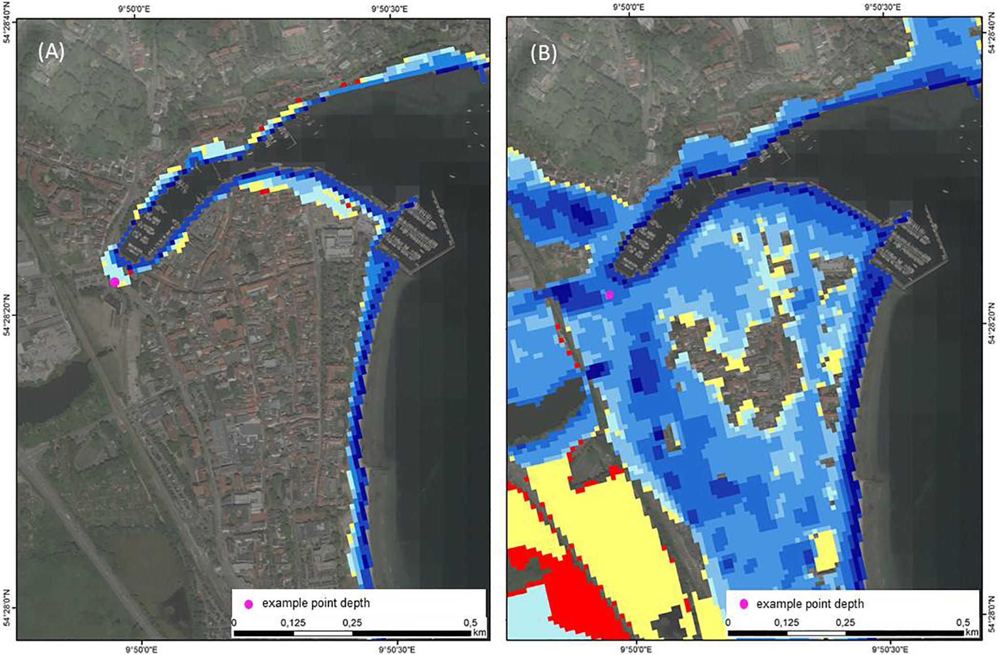
Figure 5. Flood extent simulated with Delft3D for hydrographs with water levels corresponding to a 200-year return period (A) and in combination with 1 m sea-level rise (B) in the city center of Eckernförde.

FIGURE 6

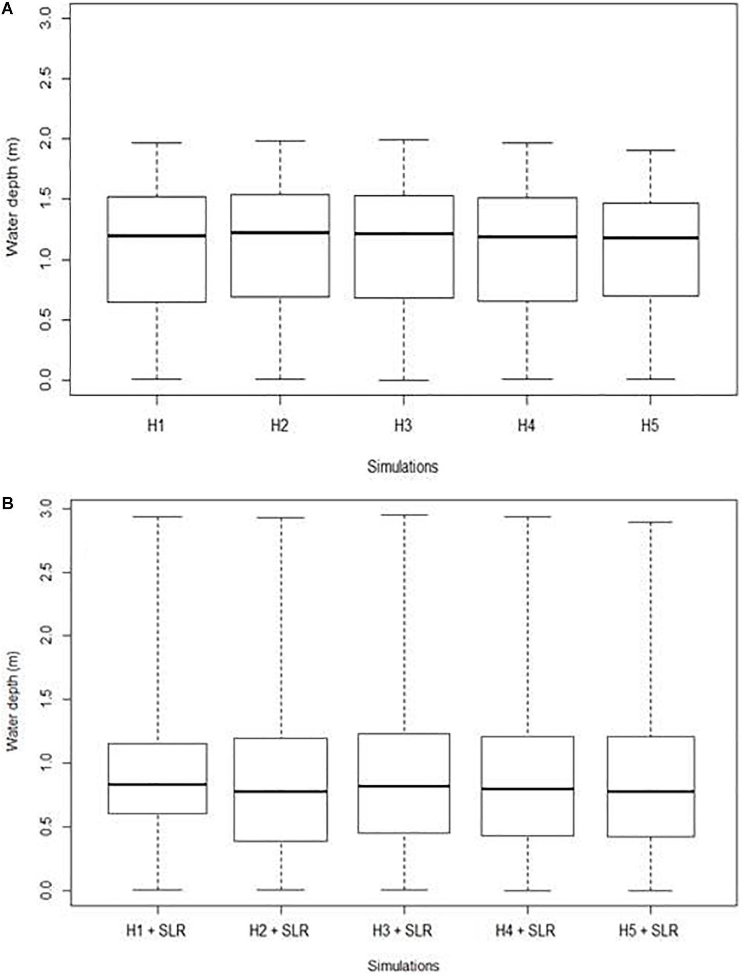
Figure 6. Flood depth for all hydrographs with water levels corresponding to a 200-year return period (A) and combined with 1 m sea-level rise (B) – The box shows values between the upper (75%) and lower (25%) quartiles. The black line inside the box indicates the median. The whiskers extent to the maximum and minimum.

The effect of storm surge temporal variability on flood impact is significantly larger when sea-level rise is considered (see Table 3 lower part). Firstly, there exists a large difference in flood extent between H1 and the other hydrographs, decreasing by 11% to H2 and 22% to H5. Differences in flood extent between H2, H3, and H4 are small, with a maximum difference of approximately four hectares. However, flood extent during H5 is approximately 10% less (13.5 hectares). These values are significantly higher than those during simulations under present sea levels, which show differences in flood extent of no more than 1.3 hectares. The number of affected properties when considering sea level rise ranges from 1,192 in H1 to 1,048 in H5. Overall, changes in inundation depth (mean and at the example point) are slightly smaller during simulations with sea-level rise. In contrast, the variances in extent are significantly larger.

Figure 7A illustrates the results for visual comparison. As the differences are hardly visible at the presented scale only three of five hydrographs are selected. Differences in extent are especially visible at the western end of the bay in the harbor area, where the majority of the buildings inside the flooded area are located. As a consequence, the change in the number of buildings exposed (ca. 18% decrease between H1 and H5) is larger than the change in flood extent. This is shown in more detail in Figure 5, which shows a close-up view of the city center of Eckernförde. Figure 7B visualizes the results for the same hydrographs but with sea level rise included in the simulations. Flood waters during H4 and H1 extend west of the city center (Figure 7B: yellow colored), where land use classification show mostly green urban areas (allotment gardens) and wetlands. Flooding which occurs only during H1 (Figure 7B: red colored) is mostly located around the Windebyer Noor, an inland lake west of Eckernförde. Flood extent also increases in areas inside the city center when comparing to H5. Overall, for the simulations including sea-level rise, deviations in the number of buildings flooded are smaller than the deviations in extent, as variations in extent mostly cover areas which are not classified as urban and thus have a lower density of buildings.

FIGURE 7

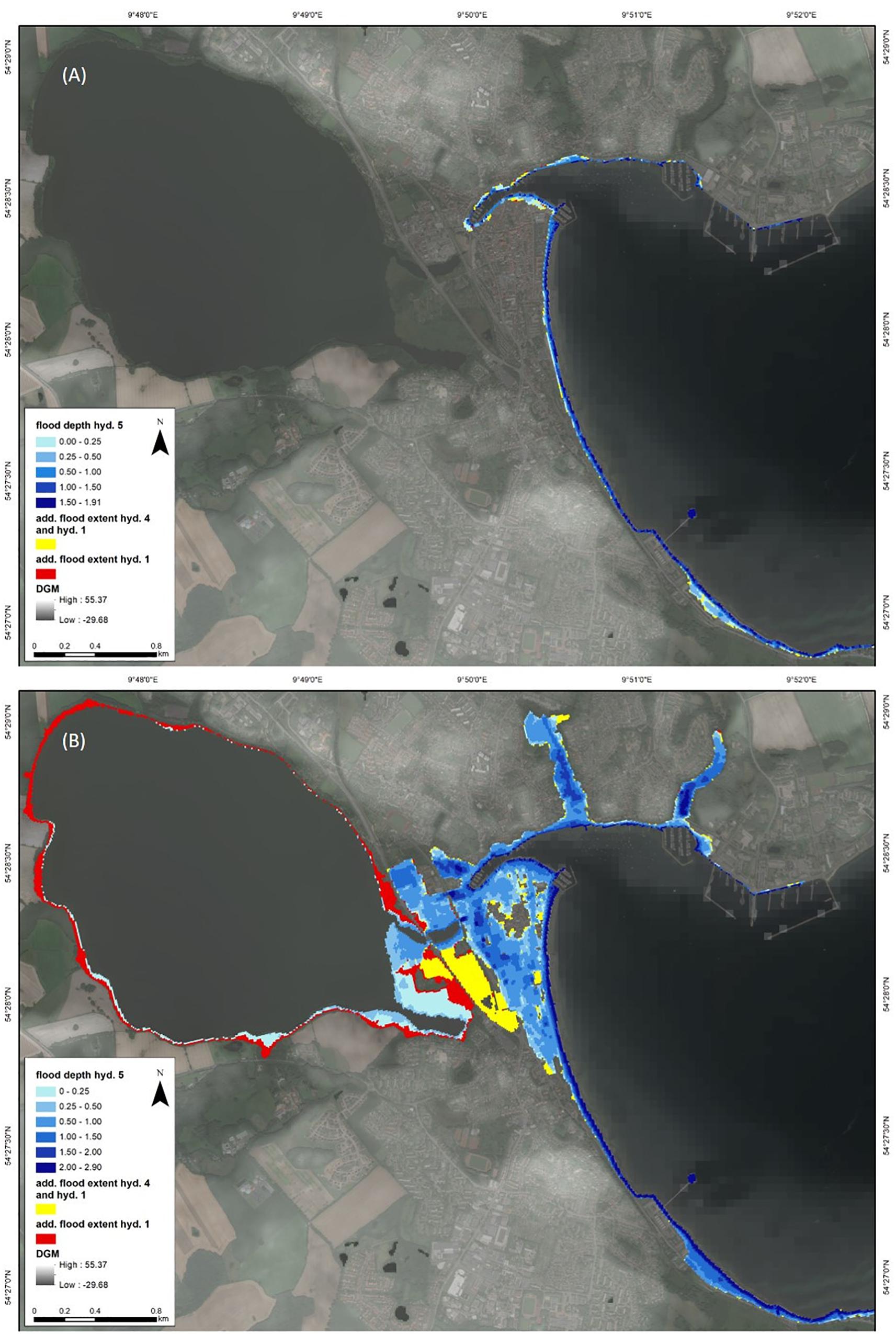
Figure 7. Flood extent simulated with Delft3D for hydrographs with water levels corresponding to a 200-year return period (A) and in combination with 1 m sea-level rise (B). The areas visualized in blue represent the flood extent of H5. The yellow colored pixels indicate the additional extent flooded in the simulation of H4 and H1. The red pixels display the extent only flooded in the case of H1.

A large increase in flood extent due to sea-level rise can be seen in Figures 5, 7. Whereas flood extent for a storm surge with a 200-year return period is 21.38 ha (H1), and limited to areas along the coastline, inundation extends further into the city center and surrounding areas when 1 m of sea-level rise is added. Here, water levels reach a peak of 2.985 m. In comparison to simulations with no sea level rise, flood extent increases by more than 500% (H5) to 630% (H1), resulting in a maximum area of inundation of 156.23 ha. The number of affected properties increases by a far greater rate from 60 to 1192 (H1). The southern part of the model domain is less affected by these changes. Most of the flooding appears in central parts of the model domain, around and south of the narrowing end of the bay (city center), which include mostly urban areas with a high density of buildings. Furthermore, the inundation reaches into two depressions at the northern side of the bay. Large areas in these parts experience inundation depths over 1 m.

Sensitivity to Manning’s Roughness Coefficients

Estimates of flood characteristics are not highly sensitive to changes in the model’s roughness coefficients. Changes account for approximately 3% difference in flood extent (calculated by number of pixels) (see Table 4) and around 2.75% in mean inundation depth. The total range of inundation depth differs by less than 1 cm. The largest differences occur when either the highest or lowest Manning roughness coefficients are used (Table 4). Modification of roughness coefficients based on the three land use classes (forest, urban, and wetland) results in a larger flood extent and smaller mean inundation depth for low roughness values and smaller extent and larger mean depth for high values. If mean values are selected, the use of varying roughness values dependent on land use produces similar results in terms of flood extent and depth to the two-part classification, where coefficients were determined for only land surfaces and water surfaces (see Table 4). Hence, the medium varying roughness coefficients are used for further model setups.

TABLE 4

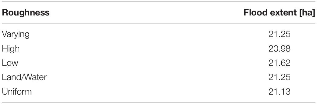
Table 4. Flood extent in case of changes in roughness coefficients.

Discussion

Model Performance and Limitations

We have set up a model of Eckernförde bay capable of simulating extreme water levels, including inundation due to extreme events. The model was validated at the Eckernförde tide gauge for two storm surge events which occurred in November of 1995 and January of 2017. RMSE and model skill for the two events indicate that the model performs well in the study area. The use of a nested model setup is a valuable tool to utilize datasets of two tide gauges with a certain distance for calibration and validation, while still obtaining detailed results for the areas of interest. The validation of the model is based on the comparison of observed and modeled water levels. Flood extent was validated using newspaper articles, which provide a qualitative evaluation of the model results. A more extensive validation of modeled flood extent and depth is not possible due to a lack of inundation data, which is a common problem when modeling inundation (Vousdoukas et al., 2018). One option to validate inundation depth is to use social media footage (e.g., photos and reports) with place and time signatures taken during a storm surge event. In such a case, inundation depth could be determined using reference objects, and used to validate points in the model domain. There are few photos of the storm surge event of 2017 available, as water overtopping the quay wall was controlled. For previous events, no visual documentation was found. Therefore, this validation procedure was not possible.

The model is not sensitive to variations in surface roughness coefficients in the study area. Mean varying Manning values found in literature reviews as well as values bisecting the area in water and land surfaces present good options. The latter might be recommendable for study areas where land use information is not available or only available at coarse resolutions. Since the model is applied on a local scale, distances are relatively small. If distances increase the sensitivity toward variations in surface roughness coefficients are expected to be larger.

The available water level records of both tide gauges are limited to a period of 27 years, which has an influence on the estimation of return water levels. Arns et al. (2013) show that 30 years of data are sufficient to estimate water levels with long return periods (>100 years). In our case, we estimate water levels with a return period of 200 years, which corresponds with the design heights of coastal protection in the region (LKN, 2013). Although this is the best estimate based on the available data, the above mentioned limitations should be carefully considered when using this value. When considering the documentation of single extreme events by WSA Lübeck (2017), which extends beyond the period of the tide gauges, three flood events over the last 150 years are equal to or greater than our estimated 200-year return water level. Therefore, we can assume that we are underestimating a 200-year water level due to these historical events. The inclusion of such historical events into the extreme value analysis is therefore important, especially when the results influence policy on flood protection. Furthermore, the magnitude of the calculated values is highly dependent on the method used. For example, in 2012 the “Ministerium für Energiewende, Landwirtschaft, Umwelt und ländliche Räume des Landes Schleswig-Holstein” (MELUR) published a value of 2.11 m for a flood with a 200-year return period in Eckernförde, whereas a value of 3.00 m was released by PROKOM GmbH (2017). This underlines the uncertainties of extreme water level estimates, which have to be outlined to avoid misinterpretation of flood characteristics based on the modeling of these extreme values.

Flood Characteristics of Temporally Variable Hydrographs

Our simulations show that variations in flood characteristics are affected by the temporal evolution of storm surge water levels. While changes in inundation depth are comparatively small for all modeled hydrographs, changes to flood extent between the different modeled hydrographs are substantial. Further, changes in flood extent are considerably larger when sea-level rise is considered. This leads to the conclusion that the temporal variability of storm surges is an important parameter to consider when conducting flood risk analyses, especially when future sea-levels are considered.

There are significant differences between H5 (shortest duration and lowest intensity: Figure 4E) and the other hydrographs with regard to both flood extent and maximum inundation depth. The change in flood extent between H1 and H5 is approximately twice as large as the difference between H1 and the other three hydrographs. Inundation depth is at least three to 9 cm lower during H5 than during all other hydrographs. This decrease is also apparent in simulations where sea-level rise is considered, which suggests a threshold of duration in which flood impact does not change substantially. If the duration of the storm surge is shorter than 40 h (such as for H5) flood extent and inundation depth is noticeably smaller. This is likely caused by declining water levels before maximum inundation depth occurs. Further research is needed to determine whether such assumptions can be validated by additional simulations and whether a possible threshold in duration can be identified.

In general, there are large differences in the flood characteristics of all five hydrographs due to the length of time at which maximum water levels are sustained. This is particularly noticeable during H1 in combination with sea-level rise. Figure 4 outlines the temporal evolution of water levels during each simulation. In H1, the water level curve is characterized by a plateau (Figure 4A), where water levels remain at the peak level for several hours. In contrast, the other hydrographs show only one clear peak (Figures 4B–E). This leads to a considerable increase in flood extent, especially when sea level rise is considered. Here, water levels do not decline immediately after the peak is reached, allowing for water to propagate further inland. In the case of the municipality of Eckernförde, mostly the lakeside and marshlands experience inundation.

Exposure to Floods and Sea-Level Rise

There is a high range of uncertainty regarding the occurrence and the development of extreme events such as storm surges and sea-level rise. In our study we investigate the consequences of two plausible scenarios in order to display the exposure of the municipality of Eckernförde to future storm surges and calculated the number of buildings intersecting the flooded area to provide insights regarding exposed infrastructure and assets. To accurately quantify potential damages, an impact assessment could be conducted by applying depth-damage functions for assets exposed to certain inundation depths (Büchele et al., 2006). Additionally, other types of infrastructure such as roads have to be regarded.

Flood exposure in Eckernförde is relatively small for the storm surges with a 200-year return period. The exposed areas (20.10–21.38 ha) are located mainly along the coastline, affecting a maximum number of 60 buildings, leading to economic damages. Since the embankment of the harbor area and also parts of the northern shore are 1.80 m (above NHN) or lower, storm surges below 2 m are capable of flooding parts of the city (PROKOM GmbH, 2017). Although events with a 200-year return period might not seem very likely to occur in the near term, the probability that events of such magnitude will be exceeded increases with regard to global sea-level rise over the century (Wahl et al., 2017).

Hydrographs simulated with 1 m sea-level rise represent examples of high-end extreme events. In their sea-level rise projections for northern Europe under RCP 8.5., Grinsted et al. (2015) highlight the development of the Antarctic ice sheet as the main source of uncertainty, which accounts for 81% of the variance in relative sea-levels. Including the risk and potential rate of Antarctic ice sheet collapse, they consider an increase in water levels of 1.70 m to be a possible high-end scenario for the western Baltic Sea in the 21st century. Such events are rare by definition, however, they are not unrealistic as higher water levels have already been observed at this location in the past. In 1872, a storm surge of 3.15 m caused immense damages and resulted in a large loss of life. Therefore, it is important that such scenarios are considered in flood risk assessment (Hinkel et al., 2015).

Our results show large parts of the city are exposed to water levels with a return period of 200 years. Exposure of the urban center of Eckernförde is especially high where the historic city center is located and the concentration of population and assets is high. Up to 1192 properties could be affected under a future sea-level rise of 1 m. Inundation depth in the city center mostly exceeds 0.5 m with large concentrations of more than 1 m depth in the western part and around the harbor. Apart from severe damages to buildings and assets, flooding can lead to traffic and transport disruption as streets become impassable. The southern and northern parts of the study area experience only little to moderate increases in flood extent. Since flooding related damages are high, people expectedly will adapt to coastal flooding and sea-level rise. In this investigation, the exposure in the municipality is calculated with the current protection level. Enhanced adaptation measures and protection schemes, in turn, should substantially reduce damages of extreme events over the next decades (Hinkel et al., 2014). This should be taken into consideration.

Conclusion

This study quantifies uncertainties in flood extent and inundation depth due to storm surge temporal variability using an inundation model in the study area Eckernförde Bay. We compared five artificial storm surge events with equal peak water levels corresponding to a return period of 200 years and varying durations and intensities, under present day and future high-end sea level rise scenarios.

Based on this analysis we conclude that under current sea levels, the effect of storm surge temporal variability is relatively small, however, this is not the case when we consider sea-level rise. Whereas differences in storm surge intensity are large (approximately 70% between H1 and H5), changes in flood extent and depth are small under present day sea levels (<10%). Such changes are significantly larger under a sea-level rise scenario of 1 m (up to 21.85%). Therefore, in consideration of projected sea-level rise until 2100, temporal variations in storm surges should be particularly reflected in future coastal flood risk assessment and management. The analysis of flood exposure shows that there is a considerable increase in flood extent when a 1 m sea-level rise scenario is combined with the scenario of a storm surge with a return period of 200 years. The specific propagation of water depends on the temporal evolution of the storm surge. This is noticeable within the urban center and further west, in the green urban areas and marshlands between the urban center and Windebyer Noor. This research can be used for further analysis, for instance, it can underpin the calculation of damages due to flooding as well as estimations on how the range of possible damages are affected by the temporal variability of extreme water level events. As the urban center of Eckernförde is not well protected against storm surges, there is a need for action to reduce potential impacts by adaptation or protection measures. These measures should not only focus on the prevention of flooding, but also on how mitigation, preparedness and response may reduce damages.

Data Availability Statement

The datasets generated for this study are available on request to the corresponding author.

Author Contributions

JH, AV, and SD designed the research. JH set up the model and collected the data, with contributions from LM. JH, AV, and LM analyzed the results. JH wrote the manuscript with contributions from AV, LM, and SD. All authors read and approved the final manuscript.

Conflict of Interest

The authors declare that the research was conducted in the absence of any commercial or financial relationships that could be construed as a potential conflict of interest.

References

Arns, A., Dangendorf, S., Jensen, J., Talke, S., Bender, J., and Pattiaratchi, C. (2017). Sea-level rise induced amplification of coastal protection design heights. Nat. Sci. Rep. 7:40171. doi: 10.1038/srep40171

PubMed Abstract | CrossRef Full Text | Google Scholar

Arns, A., Wahl, T., Haigh, D., Jensen, J., and Pattiaratchi, C. (2013). Estimating extreme water level probabilities: a comparison of the direct methods and recommendations for best practise. Coast. Eng. 81, 51–66. doi: 10.1016/j.coastaleng.2013.07.003

CrossRef Full Text | Google Scholar

Büchele, B., Kreibich, H., Kron, A., Thieken, A., Ihringer, J., Oberle, P., et al. (2006). Flood-risk mapping: contribution towards an enhanced assesssment of extreme events and associated risks. Nat. Hazards Earth Syst. Sci. 6, 485–503. doi: 10.5194/nhess-6-485-2006

CrossRef Full Text | Google Scholar

Bundesamt für Seeschifffahrt und Hydrographie (2005). Sturmflutem in der südlichen Ostsee. Berichte Des Bundesamtes Für Seeschifffahrt Und Hydrographie, 39. Rostock: Bundesamt für Seeschifffahrt und Hydrographie.

Google Scholar

Church, J. A., Clark, P. U., Cazenave, A., Gregory, J. M., Jevrejeva, S., and Levermann, A., et al. (eds) (2013). “Sea level change,” in Climate Change 2013: The Physical Science Basis. Contribution Of Working Group I to the Fifth Assessment Report of the Intergovernmental Panel on Climate Change, eds T. F. D. Stocker, G.-K. Qin, M. Plattner, S. K. Tignor, J. Allen, A. Boschung, et al. (Cambridge: Cambridge University Press), 1137–1216.

Google Scholar

Dangendorf, S., Arns, A., Pinto, J. G., Ludwig, P., and Jensen, J. (2016). The exceptional influence of storm ‘Xaver’ on design water levels in the German Bight. Environ. Res. Lett. 11:54001.

Google Scholar

Deltares (2014). Delft3D-FLOW User Manual: Simulation of Multi-Dimensional Hydrodynamic Flows and Transport Phenomena, Including Sediments. Delft: Deltares.

Google Scholar

Deltares (2018). Release Notes Delft3D Version 4.00.02. Delft: Deltares.

Google Scholar

Fisher, K., and Dawson, H. (2003). Reducing Uncertainty in River Flood Conveyance: Roughness Review. Lincoln: DEFRA.

Google Scholar

Gallien, T. W., Sanders, B. F., and Flick, R. E. (2014). Urban coastal flood prediction: integrating wave overtopping, flood defenses and drainage. Coast. Eng. 91, 18–28. doi: 10.1016/j.coastaleng.2014.04.007

CrossRef Full Text | Google Scholar

Garzon, J., and Ferreira, C. (2016). Storm surge modeling in large estuaries: sensitivity analyses to parameters and physical processes in the Chesapeake Bay. J. Mar. Sci. Eng. 4, 1–32.

Google Scholar

Gräwe, U., and Burchard, H. (2012). Storm surges in the Western Baltic Sea: the present and a possible future. Clim. Dyn. 39, 165–183. doi: 10.1007/s00382-011-1185-z

CrossRef Full Text | Google Scholar

Grinsted, A., Jevrejeva, S., Riva, R. E., and Dahl-Jensen, D. (2015). Sea level rise projections for northern Europe under RCP8.5. Clim. Res. 64, 15–23. doi: 10.3354/cr01309

CrossRef Full Text | Google Scholar

Hinkel, J., Jaeger, C., Nicholls, R. J., Lowe, J., Renn, O., and Peijun, S. (2015). Sea-level rise scenarios and coastal risk management. Nat. Clim. Chang. 5, 188–190. doi: 10.1038/nclimate2505

CrossRef Full Text | Google Scholar

Hinkel, J., Lincke, D., Vafeidis, A. T., Perrette, M., Nicholls, R. J., Tol, R. S., et al. (2014). Coastal flood damage and adaptation costs under 21st century sea-level rise. Proc. Natl. Acad. Sci. U.S.A. 111, 3292–3297. doi: 10.1073/pnas.1222469111

PubMed Abstract | CrossRef Full Text | Google Scholar

Hofstede, J. (2008). Coastal flood defence and coastal protection along the baltic sea coast of Schleswig-Holstein. Die Küste 74, 169–178.

Google Scholar

Hossain, A., Jia, Y., and Chao, X. (2009). Estimation of Manning’s Roughness Coefficient Distribution for Hydrodynamic Model Using Remotely Sensed Land Cover Features. Fairfax, VA: IEEE.

Google Scholar

IPCC (2019). “Summary for policymakers,” in IPCC Special Report on the Ocean and Cryosphere in a Changing Climate, eds H.-O. Pörtner, D. Roberts, V. Masson-Delmotte, P. Zhai, M. Tignor, E. Poloczanska, et al. (Geneva: IPCC).

Google Scholar

Jensen, J., and Müller-Navarra, S. (2008). Storm surges on the German coast. Die Küste 74, 92–124.

Google Scholar

Kühl, G. (2017). Hochwasser Hält Eckernförde in Atem. Flensburg: Eckernförder Zeitung.

Google Scholar

Landesamt für Vermessung und Geoinformation Schleswig-Holstein, (2018). Produktkatalog. Kiel: Landesamt für Vermessung und Geoinformation Schleswig-Holstein.

Google Scholar

LKN (2013). Generalplan Küstenshutz des Landes Schleswig-Holstein, Fortschreibung 2012. Kabelhorst: Landesbetrieb für Küstenschutz, Nationalpark und Meeresschutz Schleswig Holstein.

Google Scholar

MacPherson, L., Arns, A., Dangendorf, S., Vafeidis, A., and Jensen, J. (2019). A stochastic storm surge model for the German Baltic Sea coast. J. Geophys. Res. Oceans 124, 2054–2071.

Google Scholar

Martinez, G., and Bray, D. (2011). Befagung politischer Entcheidungsträger zur Wahrnehmung des Klimawandels und zur Anpassung an den Klimawandel an der deutschen Ostseeküste. Berlin: Ecologic Institut.

Google Scholar

Mignot, E., Paquier, A., and Haider, S. (2006). Modeling floods in a dense urban area using 2D shallow water equations. J. Hydrol. 327, 186–199. doi: 10.1016/j.jhydrol.2005.11.026

CrossRef Full Text | Google Scholar

Ministerium für Energiewende, Landwirtschaft, Umwelt und ländliche Räume des Landes Schleswig-Holstein (2012). Generalplan Küstenschutz des Landes Schleswig-Holstein: Fortschreibung 2012. Kiel: Ministerium für Energiewende, Landwirtschaft, Umwelt und ländliche Räume des Landes Schleswig-Holstein.

Google Scholar

Néelz, S., and Pender, G. (2013). Benchmarking the Latest Generation of 2D Hydraulic Modelling Packages. Bristol: Environment Agency.

Google Scholar

Neumann, B., Vafeidis, A. T., Zimmermann, J., and Nicholls, R. J. (2015). Future coastal population growth and exposure to sea-level rise and coastal flooding - a global assessment. PLoS One 10:e0118571. doi: 10.1371/journal.pone.0118571

PubMed Abstract | CrossRef Full Text | Google Scholar

Oregon Department of Transportation (2014). ODOT Hydraulics Manual Appendix. Salem, OR: Oregon Department of Transportation.

Google Scholar

Phillips, J., and Tadayon, S. (2006). Selection of Manning’s Roughness Coefficient for Natural and Constructed Vegetated and Non-Vegetated Channels, and Vegetation Maintenance Plan Guidelines for Vegetated Channels in Central Arizona. Virginia: U.S. Geological Survey.

Google Scholar

PROKOM GmbH (2017). Masterplan Eckernförder Bucht. Lübeck: PROKOM GmbH.

Google Scholar

Quinn, N., Lewis, M., Wadey, M., and Haigh, D. (2014). Assessing the temporal variability in extreme storm-tide time series for coastal flood risk assessment. J. Geophys. Res. Oceans 119, 4983–4998. doi: 10.1002/2014jc010197

CrossRef Full Text | Google Scholar

Rohde, C. (2017). Sturmflut: Geringe Schäden in Eckernförde. Available at: http://www.kn-online.de/Lokales/Eckernfoerde/Sturmflut-in-Eckernfoerde-Keine-groesseren-Schaeden-durch-Hochwasser (accessed September 22, 2019).

Google Scholar

Santamaria-Aguilar, S., Arns, A., and Vafeidis, A. T. (2017). Sea-level rise impacts on the temporal and spatial variabil-ity of extreme water levels: a case study for St. Peter-Ording, Germany. J. Geophys. Res. Oceans 122, 2742–2759. doi: 10.1002/2016jc012579

CrossRef Full Text | Google Scholar

Stewart, M. G., and Melchers, R. E. (1997). Probabilistic Risk Assessment of Engineering Systems. Netherlands: Springer.

Google Scholar

Technisches Hilfswerk Ortsverband Eckernförde (2017). Sturmtief Axel - Unkalkulierbare Wassermassen schwappen in Eckernförder Altstadt!. Available at: https://ov-eckernfoerde.thw.de/aktuelles/aktuelle-meldungen/artikel/sturmtief-axel-unkalkulierbare-wassermassen-schwappen-in-eckernfoerder-altstadt/ (accessed September 22, 2019).

Google Scholar

Teng, J., Jakeman, A. J., Vaze, J., Croke, B., Dutta, D., and Kim, S. (2017). Flood inundation modelling: a review of methods, recent advances and uncertainty analysis. Environ. Model. Softw. 90, 201–216. doi: 10.1016/j.envsoft.2017.01.006

CrossRef Full Text | Google Scholar

Vermeersen, B., Slangen, A., Gerkema, T., Baart, F., Cohen, K., Dangendorf, S., et al. (2018). Sea-level change in the Dutch Wadden Sea, Netherlands. J. Geosci. 97, 79–127. doi: 10.1007/s11027-015-9640-5

PubMed Abstract | CrossRef Full Text | Google Scholar

Vousdoukas, M. I., Mentaschi, L., Voukouvalas, E., Verlaan, M., Jevrejeva, S., Jackson, L. P., et al. (2018). Global probabilistic projections of extreme sea levels show intensification of coastal flood hazard. Nat. Commun. 9, 1–12. doi: 10.1038/s41467-018-04692-w

PubMed Abstract | CrossRef Full Text | Google Scholar

Vousdoukas, M. I., Voukouvalas, E., Mentaschi, L., Dottori, F., Giardino, A., Bouziotas, D., et al. (2016). Developments in large-scale coastal flood hazard mapping. Nat. Hazards Earth Syst. Sci. 16, 1841–1853. doi: 10.5194/nhess-16-1841-2016

CrossRef Full Text | Google Scholar

Wadey, M. P., Cope, S. N., Nicholls, R. J., McHugh, K., Grewcock, G., and Mason, T. (2015). Coastal flood analysis and visualisation for a small town. Ocean Coast. Manag. 116, 237–247. doi: 10.1016/j.ocecoaman.2015.07.028

CrossRef Full Text | Google Scholar

Wahl, T., Haigh, I. D., Nicholls, R. J., Arns, A., Dangendorf, S., Hinkel, J., et al. (2017). Understanding extreme sea levels for broad-scale coastal impact and adaptation analysis. Nat. Commun. 8:16075. doi: 10.1038/ncomms16075

PubMed Abstract | CrossRef Full Text | Google Scholar

Wahl, T., Mudersbach, C., and Jensen, J. (2011). Assessing the hydrodynamic boundary conditions for risk analyses in coastal areas: a stochastic storm surge model. Nat. Hazards Earth Syst. Sci. 11, 2925–2939. doi: 10.5194/nhess-11-2925-2011

CrossRef Full Text | Google Scholar

Willmott, C. J. (1984). “On the evaluation of model performance in physical geography,” in Spatial Statistics and Models. Theory and Decision Library, Vol. 40, eds Gaile, G. L., and Willmott, C. J. (Berlin: Springer), 443–460.

Google Scholar

Wong, P. P., Losada, I. J., Gattuso, J.-P., Hinkel, J., Khattabi, A., McInnes, K. L., et al. (2014). Coastal Systems and Low-Lying Areas. Climate Change 2014: Impacts, Adaptation, and Vulnerability. Part a: Global and Sectoral Aspects. Contribution of Working Group II to the Fifth Assessment Report of the Intergovernmental Panel on Climate Change. Cambridge: Cambridge University Press.

Google Scholar

WSA Lübeck (2017). Historische Wasserstände - Pegel Eckernförde. Available at: https://www.wsv.de/wsa-hl/wasserstrassen/gewaesserkunde/historisch/pdf/Eckernfoerde.pdf (accessed September 22, 2019).

Google Scholar